COMSOL Multiphysics® 4.3a

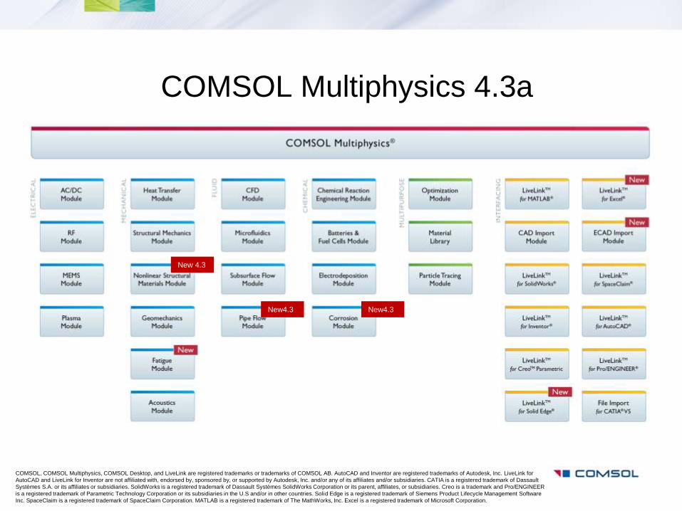
COMSOL Multiphysics 4.3a

COMSOL, COMSOL Multiphysics, COMSOL Desktop, and LiveLink are registered trademarks or trademarks of COMSOL AB. AutoCAD and Inventor are registered trademarks of Autodesk, Inc. LiveLink for

AutoCAD and LiveLink for Inventor are not affiliated with, endorsed by, sponsored by, or supported by Autodesk, Inc. and/or any of its affiliates and/or subsidiaries. CATIA is a registered trademark of Dassault

Systèmes S.A. or its affiliates or subsidiaries. SolidWorks is a registered trademark of Dassault Systèmes SolidWorks Corporation or its parent, affiliates, or subsidiaries. Creo is a trademark and Pro/ENGINEER

is a registered trademark of Parametric Technology Corporation or its subsidiaries in the U.S and/or in other countries. Solid Edge is a registered trademark of Siemens Product Lifecycle Management Software

Inc. SpaceClaim is a registered trademark of SpaceClaim Corporation. MATLAB is a registered trademark of The MathWorks, Inc. Excel is a registered trademark of Microsoft Corporation.

New 4.3

New4.3 New4.3

New Products

• Nonlinear Structural Materials Module • Nonlinear material models for structural mechanics.

• Elastoplastic, hyperelastic, viscoplastic, and creep material models.

• Large strain plastic deformation.

• Pipe Flow Module • 1D flow, heat, and mass transport in 2D and 3D pipe networks.

• Direct coupling between pipe flow and volumetric CFD.

• Pipe cross-sections, friction models, valves, pumps, elbows, T-junctions.

• Corrosion Module • Corrosion and corrosion protection simulations based on electrochemical principles.

• Galvanic, pitting, and crevice corrosion.

• Cathodic protection.

Major New Features

• Geometry and Mesh – Faster meshing for imported CAD files and the LiveLink products for CAD.

– Mesh selections for creating new boundaries and domains for any imported mesh.

• Electromagnetics – AC/DC: 3D rotating machinery and automatic coil excitation.

– RF: New polar plots for far field in 2D and 3D.

• Structural Mechanics – New nonlinear solver for mechanical contact and highly nonlinear simulations.

– Load cases for easy setup of multistep simulations.

• CFD – Turbulent mixing for mass transport simulations.

• Heat Transfer – Solar irradiation from latitude, longitude, date, and time.

• Particle Tracing – Brownian force and particle-particle interactions.

– Secondary emission and sticking probabilities.

Nonlinear Structural Materials Module

• Description: – Nonlinear Material Models for Structural

Mechanics and MEMS.

– Add-on to the Structural Mechanics Module or

MEMS Module. A few of the listed material

models were previously available in the

Structural Mechanics and MEMS Modules.

• Applications: – Any structural deformations where

deformations are large enough or operating

conditions are such, e.g. high temperature, that

material nonlinearities become important.

Animation:

Flattening of a pipe

(animation in

presentation

mode).

Necking of a metal bar.

This example is a classical

benchmark for large strain

plastic deformation.

Flattening of a pipe

with large strain

elastoplastic

deformation.

Nonlinear Structural Materials Module

• Features & User Interfaces: – Elastoplastic Material Models

• Isotropic, Kinematic, and Perfectly Plastic

Hardening

• Large-strain plasticity, for elastic and

hyperelastic materials

• Orthotropic Hill Plasticity

• Tresca and von Mises Yield Criterion

• User-defined Flow Rules

– Viscoplastic Material Model

• Anand

– Creep Material Models

• Coble, Deviatoric, Garofalo, Nabarro-

Herring, Norton, Norton-Bailey, Potential,

User-defined, Volumetric, Weertman

– Hyperelastic Material Models

• Arruda-Boyce, Money-Rivlin: two, five, and

nine parameters, Murnaghan, Neo-

Hookean, Ogden, St Venant-Kirchhoff,

User-defined

Pipe Flow Module • Description:

– Flow, heat, and mass transport in pipe

networks.

– The pipe systems are modeled as

geometrical 1D lines or curves embedded in

2D or 3D and are created using the existing

drawing tools in COMSOL Multiphysics.

– Add-on to COMSOL Multiphysics.

• Applications: – Hydraulics

– Water distribution systems

– Energy: nuclear, hydropower, geothermal

– Cooling systems in combustion engines and

turbomachinery

– Heating systems

– Chemical process industry such as plant

distribution systems

– Oil refinery pipe systems

– Lubrication

Pipe system for geothermal

heating.

Cooling of a plastic mold of a

steering wheel – including

pipe flow in cooling channels.

Pipe Flow Module • Features & User Interfaces

– Seven Physics user interfaces:

• Pipe Flow, Single Phase

• Water Hammer

• Non-Isothermal Pipe Flow

• Heat Transfer in Pipes

• Reacting Pipe Flow*

• Transport of Diluted Species in Pipes*

• Pipe Acoustics, Transient**

*=more advanced user interfaces available when combined

with other transport modules

**=when combined with the Acoustics Module

– Bidirectional couplings can be made between pipes

and 2D and 3D solid or fluid domains, as well as

between flow, heat, and mass applications.

– Pipe cross-sections, automatic transition between

laminar and turbulent flow, surface roughness, and

different friction models.

– Preset options for valves, pumps, elbows, T-junctions.

A reactor simulation for synthesis

of phtalic anhydride under

autothermal conditions using the

Pipe Flow Module together with the

Chemical Reaction Engineering

Module.

Corrosion Module

• Description: – Corrosion and corrosion protection simulations based

on electrochemical principles.

– Galvanic, pitting, crevice corrosion, and more.

– Cathodic protection.

– Add-on to COMSOL Multiphysics.

• Applications: – Corrosion and corrosion protection of:

• Off-shore structures such as oil rigs

• Ships and submarines

• Civil-engineering structures

• Chemical process industry equipment

• Automotive parts

• Mechanical structures in aerospace applications

Galvanic corrosion of a

Magnesium Alloy (AE44) - mild

steel couple in brine solution (salt

water). The electrode material

removal is represented with a

moving mesh.

Corrosion Module

• Features & User Interfaces: – Primary, Secondary, and Tertiary Current

Distribution

– Corrosion and Moving Mesh:

• Secondary Currents

• Tertiary Currents, Nernst-Planck Equation

– Thin shell electrodes

– Influence of material transport and material

concentration on corrosion and corrosion

protection including diffusion, migration and

fluid flow effects

– Include effects of heat transfer on material

transport and corrosion rates

– AC impedance simulations

Major News in COMSOL Multiphysics 4.3a

• New Products:

– LiveLink™ for Excel®:

• Run COMSOL simulations from Microsoft™ Excel®.

– Fatigue Module:

• Mechanical fatigue based on stress or strain

evaluations.

– ECAD Import Module:

• Import of ECAD layouts with new functionality for

easy filtering of cells, nets, and layers.

– LiveLink™ for Solid Edge®:

• Bidirectional associativity with Solid Edge.

• Support for cloud computing with Amazon

Elastic Compute Cloud™ (Amazon EC2™).

• Parameter optimization – Optimize on geometric dimensions and other

parameters.

• More efficient CFD solvers.

• Faster multicore and cluster computing.

LiveLink™ for Excel®

• Run COMSOL Multiphysics simulations from

an Excel spreadsheet:

– Adds a COMSOL-specific toolbar to the Excel

ribbon for displaying geometry and mesh as well

as running a simulation

– Visualize COMSOL Multiphysics results in

Excel.

– Display and edit only the most important

simulation parameters

• Synchronize or import/export parameters and

variables between Excel and COMSOL

Multiphysics:

– Interactive 3D visualizations are presented in a

separate dedicated canvas

• Excel 2007 and 2010 for Windows is

supported

Excel is a registered trademark of Microsoft Corporation.

How Does it Work?

Establishes a two-way connection between COMSOL and Excel

parameters, variables etc.

XLSX-files

parameters, variables etc.

COMSOL

Model window parameters, variables, results etc.

Excel

Excel

Load/Save Data to/from the COMSOL Desktop

• Load/save data:

– Parameters

– Variables

– Functions

COMSOL Tab and Toolbar

• A COMSOL toolbar is used to

interact with the COMSOL Model

from Excel

– Retrieve and update parameters,

variables, and functions

– Compute the model

– Show results as graphics and import

COMSOL images into Excel

– Extract numerical data to Excel

worksheets

The COMSOL Model Window

• The COMSOL Model window

– Contains the model in memory

– Shows interactive graphics

– Gets commands from the

COMSOL toolbar

Platforms

• Excel 2007 and Excel 2010 are supported

• Only Windows is supported

• Both COMSOL and Excel have 32-bit and 64-bit versions

– Many users choose to install the 32-bit version of Excel even on 64-bit

computers

– LiveLink for Excel works with any combination of Comsol and Excel

Benefits

• Ease-of-use in organizations that regularly base their data handling

on data stored in Excel

• Use Excel as a customized user interface for (complicated)

COMSOL models

• Allows the combined presentation of inputs and outputs e.g. for

reporting

Fatigue Module

• Fatigue = structural damage from repeated loading

and unloading.

• Stress levels aren’t providing enough information.

• Need Fatigue Life

– Number of load cycles before structural failure.

• Fatigue is probabilistic – statistical methods

needed.

• Add-on to the Structural Mechanics Module.

Fatigue Life Plot

Available Fatigue Evaluation Methods

* Available with the Nonlinear Structural Materials Module

ECAD Import Module

• Import of 2D layouts

– Automatic conversion of 2D layers into

3D CAD models.

– Filtering of individual cells, nets, and

layers with settings stored on file.

• Use ECAD data for any type of physics

simulation

• Supported ECAD formats

– GDS-II

– ODB++(X)

– NETEX-G

• Part of this functionality was previously

available in the AC/DC, RF, and MEMS

Modules. License holders of these modules

will get the ECAD Import Module free of

charge until next subscription renewal.

Capacitance and

inductance extraction for a

planar transformer model

imported as an ECAD file.

LiveLink™ for Solid Edge®

• Solid Edge® is a CAD software provided by Siemens PLM®.

• The LiveLink™ for Solid Edge® offers fully associative integration with Solid

Edge for multiphysics simulations involving parametric sweeps and

design optimization.

• Contains the functionality of the CAD Import Module.

Solid Edge is a registered trademark of Siemens Product Lifecycle Management Software Inc.

Corrosion potential of an

oil rig structure surrounded

by 52 sacrificial anodes

Cloud Computing

• Run simulations on Amazon Elastic

Compute Cloud™ (Amazon EC2™).

– Access high-end hardware on a pay-per-

use basis.

• Types of computations:

– Multicore Computing on one virtual

computer with lots of RAM.

– Cluster Sweep for parallel parametric

studies.

– Cluster Computing for large distributed

memory simulations.

• New remote access tools:

– Optimized data transfer to minimize

upload/download of data.

– Dial-back to on-premise license manager.

– Run from GUI or batch mode.

• Available for any COMSOL Multiphysics

user with a Floating Network License.

The new user

interfaces for Remote

Access.

Amazon EC2 and Amazon Elastic Compute Cloud are trademarks of Amazon Web Services, LLC or its affiliates.

SSH

Tunnel

Port forwarding

Cloud Computing Setup

Local desktop

computer

Local license

server

The Cloud

Data License

info

Cloud Computing Setup

• Open an Amazon AWS Account

• Install either PuTTY or use local linux installation

• Start an, or several Amazon Cloud Entity(ies) dependent on the

size/type of job

– High Memory

– High CPU

– HPC (both of the above)

• Upload local installation(typically once, but has to include all files

except from doc and model library)

• Run job, as you would do on your local cluster

• Terminate when finished.

Cloud computing setup

• Tips and tricks

– Read the manual(!)

– Use StarCluster-software from MIT to

run the Amazon cluster entities (Free)

• star.mit.edu/cluster/

– Test with free usage tier before

running your BIG model.(max 500MB

of memory..)

Swifter Parallel Computing

• More efficient parallel computing for both shared-memory/multicore and distributed

computing.

• Multicore computing:

• Greatly improved handling of constraint boundary conditions such as fixed temperature,

electric potential, and displacement speeds up computations for most physics.

Performance increase is thanks to new constraint elimination algorithms.

• Distributed computing:

• Solvers have been optimized by the introduction of a very efficient sparse matrix reordering

algorithm for direct solvers.

• Communication for matrix-vector data has been optimized.

An evanescent-mode

cavity filter.

Parameter Optimization

• Gradient-free parameter

optimization can now be applied

due to three new optimization

methods:

– Nelder-Mead.

– Coordinate Search.

– Monte Carlo.

• Optimize with respect to one or

more geometric dimensions: – for a CAD model created directly with

COMSOL Multiphysics.

– for a model from a CAD package linked

through any of the LiveLink™ products.

• Parameter optimization is not

limited to geometric dimensions but

can be applied to any parameters of

a model.

Tunable MEMS capacitor

where a target capacitance

of 0.1 pF is found by

optimizing the distance

between capacitor plates.

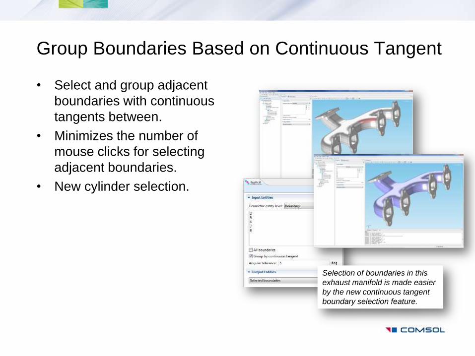
Group Boundaries Based on Continuous Tangent

• Select and group adjacent

boundaries with continuous

tangents between.

• Minimizes the number of

mouse clicks for selecting

adjacent boundaries.

• New cylinder selection.

Selection of boundaries in this

exhaust manifold is made easier

by the new continuous tangent

boundary selection feature.

Logical Expression-based Mesh Selection

• Based on Coordinate Variables:

– Use the x, y, and z coordinate variables in a logical expression, such as

(y<-40)&&(z>2.5) to partition an imported mesh into new domains or boundaries.

• Visualization of coordinate box and ball.

Partitioning a mesh based on a

logical expression in terms of

coordinate variables x, y, and z.

Geometry Modeling: Import of Contour Plots

• Contour plots can now be

exported on the Sectionwise

data format:

– allows them to be imported and

reused as an interpolation curve in a

geometry model

– this enables contour plots to be part

of a 2D or 3D geometry model

– 2D curves can be extruded,

revolved, or swept into 3D geometry

objects.

An isothermal contour line is

imported as an interpolation

curve, extruded, and used to

partition this geometry of a

power transistor and circuit

board.

Tailored Mesh Settings for CFD

• Automatic corner refinement.

• Splitting at sharp corners

instead of trimming.

• Robust and accurate for larger

geometry models.

• Integrated with multigrid solver

for CFD.

A boundary layer mesh with

automatic corner refinement and

new handling of sharp edges.

FLUID

One-Way Coupled Fluid-Structure Interaction (FSI)

• Solving for One-way Coupled FSI is

more efficient when there is no coupling

from the structure back on to the fluid

(i.e., no ”flexing back”)

• New study types for FSI:

– Stationary, One-way Coupled

– Time-dependent, One-way Coupled

• Solves for the fluid first, then for the

structure.

• Other physics can be included in either

or both study steps.

• Requires Structural Mechanics or

MEMS Module.

More Robust and Easier-to-use Pseudo Time-

Step Solver for Stationary CFD and FSI

• Pseudo-time stepping is used for robust convergence towards steady-state solution:

– Available for all stationary flow physics user interfaces and FSI.

– Faster solutions for simple models.

– More robust behavior for large models.

• CFL number controlled by a new PID regulator:

– Instead of built-in expression.

– Much easier to tune.

• Pseudo time-derivative removed from continuity equation:

– Removes models that ”resonate”.

– More robust.

Much Improved Default Solver for CFD

• Implemented for all flow interfaces. – Reduced memory requirements for large models.

– More automation and less manual tuning.

• Mesh building triggered when

retrieving default solvers: – This shows when default solvers take longer.

• Direct solver for small models:

– Small is 100,000 elements in 3D and

300,000 elements in 2D

• Default geometric multigrid (GMG)

solver automatically adjusted based

on the number of mesh elements.

• Additional multigrid levels are

automatically added for large models: – First additional level at 600,000 elements

– Maximum of four levels including the finest

mesh for first order elements. Additional

levels for higher-order elements.

Reacting Flow User Interface

• New Reacting Flow User Interface for

Laminar and Turbulent Mass Transport:

– Combination of Laminar or Turbulent Single-

phase Flow with Transport of Concentrated

Species.

– Includes turbulent wall functions for mass

transport, turbulent reaction modeling, and

reaction kinetics.

• Built-in algebraic models automatically

computes the Schmidt number.

• Also features turbulent low-Reynolds mass

transport for high Schmidt number (for

reactions in liquids).

• Based on the so called Eddy Dissipation

Concept (EDC).

Moist Air Fluid Model

• Heat Transfer in Fluids now

contains a new Moist air fluid

type:

– Contains thermodynamics properties of

unsaturated humid air.

– Dedicated postprocessing variables.

• Verify if the saturation level has

been reached during the

simulation.

• Available in the Heat Transfer

Module

MECHANICAL

Load Cases for Heat Transfer

• Loads and constraints for heat transfer is

now available using the same load and

constraint group concept as in the

Structural Mechanics Module.

• Use load groups for heat sources and

heat fluxes.

• Use constraint groups for temperature

conditions.

New Hyperelastic Material Models

• Nonlinear Structural Materials

Module comes with three new

hyperelastic material models:

– Yeoh

– Varga:

• Nearly incompressible, nonlinear

elastic materials such as rubber.

– Blatz-Ko:

• Highly compressible materials such

as foam rubber.

Acoustics Module

• New tutorial model of the Brüel & Kjær

4134 condenser microphone:

– Compares the simulated sensitivity level

to measurements performed on an actual

microphone.

• New Boundary layer approximation fluid

model for pressure acoustics:

– allows for simulation of the thermal and

viscous losses at boundaries of a duct as

a bulk loss (an equivalent fluid).

• The viscous characteristic length can

now be entered directly in the Biot

equivalent fluid models.

• The Thermoacoustics user interface

now features a heat source option which

is used for optoacoustics and acoustic

heat exchangers.

Model geometry and

measurement courtesy of

Brüel & Kjær Sound &

Vibration Measurement A/S,

Nærum, Denmark.

CHEMICAL

Film Resistance

• Used for resistance modeling

in electrochemical

applications:

– Passivation.

– Growing oxide layers

– etc.

• Introduced for all boundary

conditions that model an

interface between an

electrolyte and an electrode.

• Available in the Corrosion,

Electrodeposition, and

Batteries & Fuel Cells

Modules

Equation

New Section

(No film resistance

is default)

ELECTRICAL

RF Module

• A new general 2.5D formulation for waves

– Use for disk antenna modeling, accurate scattering modeling,

laser (Gaussian) beam models, and cavity model analysis for

accelerators, for example.

• Dedicated port for periodic structures in 2D models.

– Easier to model excitation of Floquet periodic structures and

includes automatic setup of diffraction orders.

• Support for volumetric currents

– Set a volumetric external current density in domains.

MULTIPURPOSE

Particle Tracing Module

• New boundary conditions are available for the following types of

particle reflections:

• Diffuse reflection.

• General reflection, where you can supply your own expressions for the

particle velocity after collisions with a wall.

• Pass through, which can be used on interior boundaries in conjunction with

a sticking probability or expression.

• New variables have been added for the particle release time,

particle stop time, and particle status.

• Now possible to specify a logical expression for the particle to

include in the Filter subnode for the Particle Trajectories plot.