Computing the Stationary Distribution, Locally · 2015-05-04 · Lee, Ozdaglar, and Shah: Local...
49
Submitted to Operations Research manuscript (Please, provide the manuscript number!) Computing the Stationary Distribution, Locally Christina E. Lee, Asuman Ozdaglar, Devavrat Shah Laboratory for Information and Decision Systems, Massachusetts Institute of Technology, Cambridge, MA 02139, [email protected], [email protected], [email protected] Computing the stationary distribution of a large finite or countably infinite state space Markov Chain has become central to many problems such as statistical inference and network analysis. Standard methods involve large matrix multiplications as in power iteration, or simulations of long random walks, as in Markov Chain Monte Carlo (MCMC). For both methods, the convergence rate is is difficult to determine for general Markov chains. Power iteration is costly, as it is global and involves computation at every state. In this paper, we provide a novel local algorithm that answers whether a chosen state in a Markov chain has stationary probability larger than some Δ ∈ (0, 1), and outputs an estimate of the stationary probability for itself and other nearby states. Our algorithm runs in constant time with respect to the Markov chain, using information from a local neighborhood of the state on the graph induced by the Markov chain, which has constant size relative to the state space. The multiplicative error of the estimate is upper bounded by a function of the mixing properties of the Markov chain. Simulation results show Markov chains for which this method gives tight estimates. Key words : Markov chains, stationary distribution, local algorithms, network centralities 1. Introduction Computing the stationary distribution of a Markov chain with a very large state space (finite, or countably infinite) has become central to statistical inference. The ability to tractably simulate Markov chains along with its generic applicability has made Markov Chain Monte Carlo (MCMC) arguably one of the top algorithms of the twentieth century (Cipra 2000). However, MCMC and its variations suffer from limitations in large state spaces, as they involve sampling states from long random walks over the entire state space (Metropolis et al. 1953, Hastings 1970). It is difficult to determine for general Markov chains when the algorithm has walked “long enough” to produce reasonable approximations for the stationary distribution. This has motivated the development of super-computation capabilities – be it nuclear physics (Semkow et al. 2006, Chapter 8), Google’s computation of PageRank (Page et al. 1999), or stochastic simulation at-large (Assmussen and Glynn 2010). Stationary distributions of Markov chains are also central to network analysis. Networks have become ubiquitous representations for capturing interactions and relationships between entities across many disciplines, including social interactions between individuals, interdependence between 1
Transcript of Computing the Stationary Distribution, Locally · 2015-05-04 · Lee, Ozdaglar, and Shah: Local...

Submitted to Operations Researchmanuscript (Please, provide the manuscript number!)
Computing the Stationary Distribution, Locally
Christina E. Lee, Asuman Ozdaglar, Devavrat ShahLaboratory for Information and Decision Systems, Massachusetts Institute of Technology, Cambridge, MA 02139,
[email protected], [email protected], [email protected]
Computing the stationary distribution of a large finite or countably infinite state space Markov Chain has
become central to many problems such as statistical inference and network analysis. Standard methods
involve large matrix multiplications as in power iteration, or simulations of long random walks, as in Markov
Chain Monte Carlo (MCMC). For both methods, the convergence rate is is difficult to determine for general
Markov chains. Power iteration is costly, as it is global and involves computation at every state. In this paper,
we provide a novel local algorithm that answers whether a chosen state in a Markov chain has stationary
probability larger than some ∆∈ (0,1), and outputs an estimate of the stationary probability for itself and
other nearby states. Our algorithm runs in constant time with respect to the Markov chain, using information
from a local neighborhood of the state on the graph induced by the Markov chain, which has constant size
relative to the state space. The multiplicative error of the estimate is upper bounded by a function of the
mixing properties of the Markov chain. Simulation results show Markov chains for which this method gives
tight estimates.
Key words : Markov chains, stationary distribution, local algorithms, network centralities
1. Introduction
Computing the stationary distribution of a Markov chain with a very large state space (finite, or
countably infinite) has become central to statistical inference. The ability to tractably simulate
Markov chains along with its generic applicability has made Markov Chain Monte Carlo (MCMC)
arguably one of the top algorithms of the twentieth century (Cipra 2000). However, MCMC and
its variations suffer from limitations in large state spaces, as they involve sampling states from
long random walks over the entire state space (Metropolis et al. 1953, Hastings 1970). It is difficult
to determine for general Markov chains when the algorithm has walked “long enough” to produce
reasonable approximations for the stationary distribution. This has motivated the development of
super-computation capabilities – be it nuclear physics (Semkow et al. 2006, Chapter 8), Google’s
computation of PageRank (Page et al. 1999), or stochastic simulation at-large (Assmussen and
Glynn 2010).
Stationary distributions of Markov chains are also central to network analysis. Networks have
become ubiquitous representations for capturing interactions and relationships between entities
across many disciplines, including social interactions between individuals, interdependence between
1
Lee, Ozdaglar, and Shah: Local Stationary Distribution2 Article submitted to Operations Research; manuscript no. (Please, provide the manuscript number!)
financial institutions, hyper-link structure between web-pages, or correlations between distinct
events. Many decision problems over networks rely on information about the importance of differ-
ent nodes as quantified by network centrality measures. Network centrality measures are functions
assigning “importance” values to each node in the network. The stationary distribution of specific
random walks on these underlying networks are used as network centrality measures in many set-
tings. A few examples include PageRank: which is commonly used in Internet search algorithms
(Page et al. 1999), the Bonacich centrality and eigencentrality measures: encountered in the analy-
sis of social networks (Newman 2010, Candogan et al. 2012, Chasparis and Shamma 2010), rumor
centrality: utilized for finding influential individuals in social media like Twitter (Shah and Zaman
2011), and rank centrality: used to find a ranking over items within a network of pairwise compar-
isons (Negahban et al. 2012).
1.1. Contributions
In this paper, we provide a novel algorithm that addresses these limitations1. Our algorithm answers
the following question: for a given node i of a countable state space Markov chain, is the stationary
probability of i larger than a given threshold ∆ ∈ (0,1), and can we approximate it? For chosen
parameters ∆, ε, and α, our algorithm guarantees that for nodes such that the estimate πi <
∆/(1 + ε), the true value πi is also less than ∆ with probability at least 1−α. In addition, if πi ≥
∆/(1 + ε), with probability at least 1−α, the estimate is within an ε times Zmax(i) multiplicative
factor away from the true πi, where Zmax(i) is effectively a “local mixing time” for i derived from
the fundamental matrix of the transition probability matrix P . The algorithm also gives estimates
for other nodes j within the vicinity of node i. The estimation error depends on the mixing and
connectivity properties of node i and node j.
The running time of the algorithm is upper bounded by O (ln(1/α)/ε3∆), which is constant
with respect to the Markov chain2. Our algorithm uses only a“local neighborhood” of the state i,
defined with respect to the Markov graph, which is constructed using the transition probabilities
betwen states. Stopping conditions are easy to verify and have provable performance guarantees.
Its construction relies on a basic property: the stationary probability of each node is inversely
proportional to the mean of its “return time.” Therefore, we sample return times to the node and
use the empirical average as an estimate. Since return times can be arbitrarily long, we truncate
sample return times at a chosen threshold. Hence, our algorithm is a truncated Monte Carlo method.
We also use these samples to obtain estimates to other nodes j by observing the frequency of visits
to node j within a return path to node i.
We utilize the exponential concentration of return times in Markov chains to establish theoretical
guarantees for the algorithm. For countably infinite state space Markov chains, we build upon a
Lee, Ozdaglar, and Shah: Local Stationary DistributionArticle submitted to Operations Research; manuscript no. (Please, provide the manuscript number!) 3
result by Hajek (1982) on the concentration of certain types of hitting times to derive concentration
of return times to a given node. We use these concentration results to upper bound the estimation
error and the algorithm runtime as a function of the truncation threshold and the mixing prop-
erties of the graph. For graphs that mix quickly, the distribution over return times concentrates
more sharply around its mean, resulting in tighter performance guarantees. We illustrate the wide
applicability of our local algorithm for computing network centralities and stationary distributions
of queuing models.
1.2. Related Literature
We provide a brief overview of the standard methods used for computing stationary distributions.
1.2.1. Monte Carlo Markov Chain Monte Carlo Markov chain methods involve simulating
long random walks over a carefully designed Markov chain in order to obtain samples from a target
stationary distribution (Metropolis et al. 1953, Hastings 1970). After the length of this random
walk exceeds the mixing time, the distribution over the current state of the random walk will be a
close approximation to the stationary distribution. Thus, the observed current state of the random
walk is used as an approximate sample from π. This process is repeated many times to collect
independent samples from πi. Articles by Diaconis and Saloff-Coste (1998) and Diaconis (2009)
provide a summary of the major development from probability theory perspective.
The majority of work following the initial introduction of this method involves analyzing the
convergence rates and mixing times of the random walk over different Markov chains (Aldous and
Fill 1999, Levin et al. 2009). Techniques involve spectral analysis or coupling arguments. Graph
properties such as conductance provide ways to characterize the spectrum of the graph. Most results
are limited to reversible finite state space Markov chains, which are equivalent to random walks on
weighted undirected graphs. For general non-reversible countable state space Markov chains, little
is known about the mixing time, and thus many practical Markov chains lack precise convergence
rate bounds.
1.2.2. Power Iteration The power-iteration method (see Golub and Van Loan (1996), Stew-
art (1994), Koury et al. (1984)) is an equally old and well-established method for computing leading
eigenvectors of matrices. Given a matrix A and a seed vector x0, recursively compute iterates
xt+1 =Axt/‖Axt‖. If matrix A has a single eigenvalue that is strictly greater in magnitude than
all other eigenvalues, and if x0 is not orthogonal to the eigenvector associated with the dominant
eigenvalue, then a subsequence of xt converges to the eigenvector associated with the dominant
eigenvalue. Recursive multiplications involving large matrices can become expensive very fast as the
matrix grows. When the matrix is sparse, computation can be saved by implementing it through
Lee, Ozdaglar, and Shah: Local Stationary Distribution4 Article submitted to Operations Research; manuscript no. (Please, provide the manuscript number!)
‘message-passing’ techniques; however it still requires computation to take place at every node in
the state space. The convergence rate is governed by the spectral gap, or the difference between
the two largest eigenvalues. Techniques used for analyzing the spectral gap and mixing times as
discussed above are also used in analyzing the convergence of power iteration. For large Markov
chains, the mixing properties may scale poorly with the size, making it difficult to obtain good
estimates in a reasonable amount of time. As before, most results only pertain to reversible Markov
chains.
In the setting of computing PageRank, there have been efforts to modify the algorithm to execute
power iteration over local subsets of the graph and combine the results to obtain estimates for
the global PageRank. These methods rely upon key assumptions on the underlying graph, which
are difficult to verify. Kamvar et. al. observed that there may be obvious ways to partition the
web graph (i.e. by domain names) such that power iteration can be used to estimate the local
PageRank within these partitions (Kamvar et al. 2003). They use heuristics to estimate the relative
weights of these partitions, and combine the local PageRank within each partition according to
the weights to obtain an initial estimate for PageRank. This initial estimate is used to initialize
the power iteration method over the global Markov chain, with the hope that this initialization
may speed up convergence. Chen et. al. proposed a method for estimating the PageRank of a
subset of nodes given only the local neighborhood of this subset (Chen et al. 2004). Their method
uses heuristics such as weighted in-degree as estimates for the PageRank values of nodes on the
boundary of the given neighborhood. After fixing the boundary estimates, standard power iteration
is used to obtain estimates for nodes within the local neighborhood. The error in this method
depends on how close the true PageRank of nodes on the boundary correspond to the heuristic
guesses such as weighted in-degree. Unfortunately, we rarely have enough information to make
accurate heuristic guesses of these boundary nodes.
1.2.3. Computing PageRank Locally There has been much recent effort to develop local
algorithms for computing PageRank for the web graph. Given a directed graph of n nodes with
an n×n adjacency matrix A (i.e., Aij = 1 if (i, j)∈E and 0 otherwise), the PageRank vector π is
given by the stationary distribution of a Markov chain over n states, whose transition matrix P is
given by
P = (1−β)D−1A+β1 · rT . (1)
D denotes the diagonal matrix whose diagonal entries are the out-degrees of the nodes; β ∈ (0,1) is
a fixed scalar; and r is a fixed probability vector over the n nodes3. In each step the random walk
with probability (1− β) chooses one of the neighbors of the current node equally likely, and with

Lee, Ozdaglar, and Shah: Local Stationary DistributionArticle submitted to Operations Research; manuscript no. (Please, provide the manuscript number!) 5
probability β chooses any of the nodes in the graph according to r. Thus, the PageRank vector π
satisfies
πT = πTP = (1−β)πTD−1A+βrT (2)
where πT · 1 = 1. This definition of PageRank is also known as personalized PageRank, because r
can be tailored to the personal preferences of a particular web surfer. When r= 1n·1, then π equals
the standard global PageRank vector. If r = ei, then π describes the personalized PageRank that
jumps back to node i with probability β in every step4.
Computationally, the design of local algorithms for computing the personalized PageRank has
been of interest since its discovery. Most of the algorithms and analyses crucially rely on the specific
structure of the random walk describing PageRank: P decomposes into a natural random walk
matrix D−1A, and a rank-1 matrix 1 · rT , with strictly positive weights (1−β) and β respectively,
cf. (1). Jeh and Widom (2003) and Haveliwala (2003) observed a key linearity relation – the global
PageRank vector is the average of the n personalized PageRank vectors corresponding to those
obtained by setting r = ei for 1≤ i≤ n. That is, these n personalized PageRank vectors centered
at each node form a basis for all personalized PageRank vectors, including the global PageRank.
Therefore, the problem boils down to computing the personalized PageRank for a given node.
Fogaras et al. (2005) used the fact that for the personalized PageRank centered at a given node
i (i.e., r = ei), the associated random walk has probability β at every step to jump back to node
i, “resetting” the random walk. The distribution over the last node visited before a “reset” is
equivalent to the personalized PageRank vector corresponding to node i. Therefore, they propose
an algorithm which samples from the personalized PageRank vector by simulating short geometric-
length random walks beginning from node i, and recording the last visited node of each sample
walk. The performance of the estimate can be established using standard concentration results.
Subsequent to the key observations mentioned above, Avrachenkov et al. (2007) surveyed variants
to Fogaras’ random walk algorithm, such as computing the frequency of visits to nodes across the
sample path rather than only the end node. Bahmani et al. (2010) addressed how to incrementally
update the PageRank vector for dynamically evolving graphs, or graphs where the edges arrive in
a streaming manner. Das Sarma et al. extended the algorithm to streaming graph models (Sarma
et al. 2011), and distributed computing models (Sarma et al. 2012), “stitching” together short
random walks to obtain longer samples, and thus reducing communication overhead. More recently,
building on the same sets of observation, Borgs et al. (2012) provided a sublinear time algorithm for
estimating global PageRank using multi-scale matrix sampling. They use geometric-length random
walk samples, but do not require samples for all n personalized PageRank vectors. The algorithm

Lee, Ozdaglar, and Shah: Local Stationary Distribution6 Article submitted to Operations Research; manuscript no. (Please, provide the manuscript number!)
returns a set of “important” nodes such that the set contains all nodes with PageRank greater than
a given threshold, ∆, and does not contain any node with PageRank less than ∆/c with probability
1− o(1), for a given c > 1. The algorithm runs in time O (n/∆).
Andersen et al. (2007) designed a backward variant of these algorithms. Previously, to compute
the global PageRank of a specific node j, we would average over all personalized PageRank vec-
tors. The algorithm proposed by Andersen et al. estimates the global PageRank of a node j by
approximating the “contribution vector”, i.e. estimating for the jth coordinates of the personalized
PageRank vectors that contribute the most to πj.
All of these algorithms rely on the crucial property that the random walk has renewal time
that is distributed geometrically with constant parameter β > 0 that does not scale with graph
size n. This is because the transition matrix P decomposes according to (1), with a fixed β. In
general, the transition matrix of any irreducible, positive-recurrent Markov chain will not have
such a decomposition property (and hence known renewal time), making the above algorithms
inapplicable in general.
2. Preliminaries: Markov Chains
Consider a discrete-time, irreducible, positive-recurrent Markov chain Xtt≥0 on a countable state
space Σ. Let P denote the transition probability matrix, and let P (n)xy denote the value of entry
(x, y) in the matrix P n. If the state space is countably infinite, then P : Σ×Σ→ [0,1] is a function
such that for all x, y ∈Σ,
Pxy = P(Xt+1 = y|Xt = x).
Similarly, P (n)xy is defined for all x, y ∈Σ to be
P (n)xy , P(Xn = y|X0 = x).
The stationary distribution is a function π : Σ→ [0,1] such that∑
i∈Σ πi = 1 and πi =∑
j∈Σ πjPji
for all i∈Σ. The stationary distribution is the quantity that we are interested in estimating, with
a focus on identifying states with large stationary probabilities.
The Markov chain can be visualized as a random walk over a weighted directed graph G =
(Σ,E,P ), where Σ is the set of nodes, E = (i, j) ∈ Σ× Σ : Pij > 0 is the set of edges, and P
describes the weights of the edges. We refer to G as the Markov chain graph. The state space Σ
is assumed to be either finite or countably infinite. If it is finite, let n= |Σ| denote the number of
nodes in the graph5.
We assume throughout this paper that the Markov chain Xt is irreducible6 and positive recur-
rent7. This guarantees that there exists a unique stationary distribution.
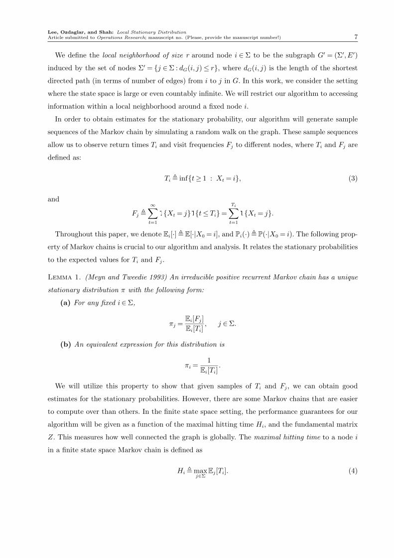
Lee, Ozdaglar, and Shah: Local Stationary DistributionArticle submitted to Operations Research; manuscript no. (Please, provide the manuscript number!) 7
We define the local neighborhood of size r around node i ∈ Σ to be the subgraph G′ = (Σ′,E′)
induced by the set of nodes Σ′ = j ∈Σ : dG(i, j)≤ r, where dG(i, j) is the length of the shortest
directed path (in terms of number of edges) from i to j in G. In this work, we consider the setting
where the state space is large or even countably infinite. We will restrict our algorithm to accessing
information within a local neighborhood around a fixed node i.
In order to obtain estimates for the stationary probability, our algorithm will generate sample
sequences of the Markov chain by simulating a random walk on the graph. These sample sequences
allow us to observe return times Ti and visit frequencies Fj to different nodes, where Ti and Fj are
defined as:
Ti , inft≥ 1 : Xt = i, (3)
and
Fj ,∞∑t=1
1Xt = j1t≤ Ti=
Ti∑t=1
1Xt = j.
Throughout this paper, we denote Ei[·],E[·|X0 = i], and Pi(·), P(·|X0 = i). The following prop-
erty of Markov chains is crucial to our algorithm and analysis. It relates the stationary probabilities
to the expected values for Ti and Fj.
Lemma 1. (Meyn and Tweedie 1993) An irreducible positive recurrent Markov chain has a unique
stationary distribution π with the following form:
(a) For any fixed i∈Σ,
πj =Ei[Fj]Ei[Ti]
, j ∈Σ.
(b) An equivalent expression for this distribution is
πi =1
Ei[Ti].
We will utilize this property to show that given samples of Ti and Fj, we can obtain good
estimates for the stationary probabilities. However, there are some Markov chains that are easier
to compute over than others. In the finite state space setting, the performance guarantees for our
algorithm will be given as a function of the maximal hitting time Hi, and the fundamental matrix
Z. This measures how well connected the graph is globally. The maximal hitting time to a node i
in a finite state space Markov chain is defined as
Hi ,maxj∈Σ
Ej[Ti]. (4)

Lee, Ozdaglar, and Shah: Local Stationary Distribution8 Article submitted to Operations Research; manuscript no. (Please, provide the manuscript number!)
The fundamental matrix Z of a finite state space Markov chain is
Z ,∞∑t=0
(P (t)−1πT
)=(I −P + 1πT
)−1,
i.e., the entries of the fundamental matrix Z are defined by
Zjk ,∞∑t=0
(P
(t)jk −πk
).
Since P(t)jk denotes the probability that a random walk beginning at node j is at node k after t
steps, Zjk represents how quickly the probability mass at node k from a random walk beginning
at node j converges to πk. We will use the following property, stated by Aldous and Fill (1999), to
relate entries in the fundamental matrix to expected return times.
Lemma 2. For j 6= k,
Ej[Tk] =Zkk−Zjk
πk.
We define Zmax(i),maxk∈Σ |Zki|. The relationship between Zmax(i) and Hi is described by
Zmax(i)≤ πiHi ≤ 2Zmax(i).
3. Problem Statement
Consider a discrete time, irreducible, positive recurrent Markov chain Xtt≥0 on a countable state
space Σ with transition probability matrix P : Σ× Σ→ [0,1]. Given node i and threshold ∆, is
πi > ∆? If so, what is πi? We provide a local approximation algorithm for πi, which uses only
edges within a local neighborhood around i of constant size with respect to the state space. We
also extend this local algorithm to give approximations for the stationary probabilities of a set of
nodes J ⊆Σ.
Definition 1. An algorithm is local if it only uses information within a local neighborhood of size
r around i, where r is constant with respect to the size of the state space.
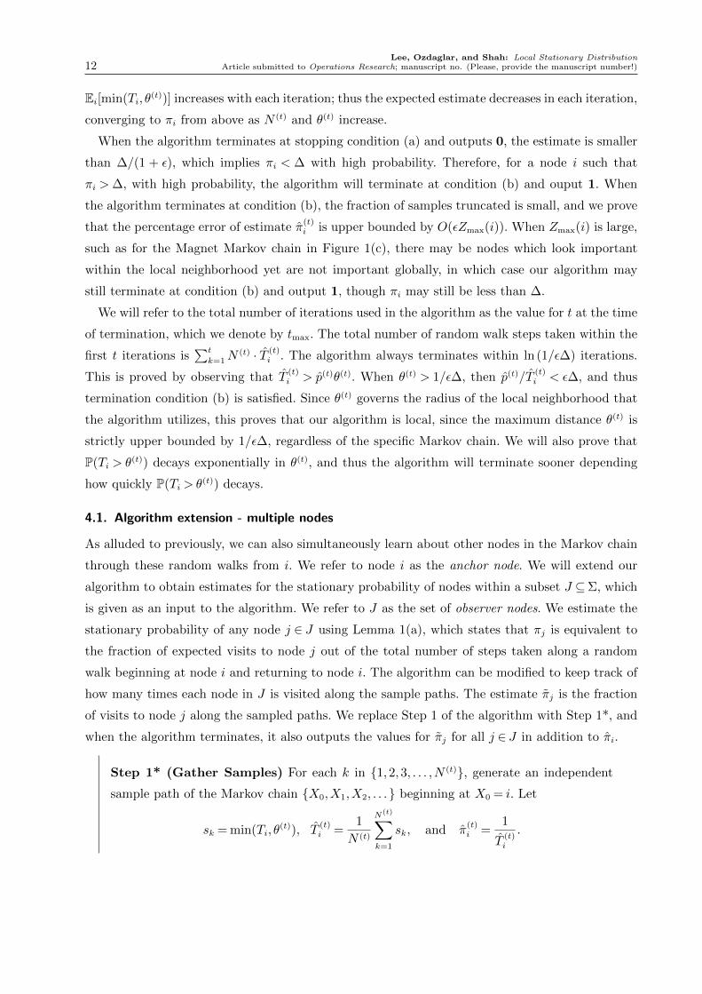
We illustrate the limitations of using a local algorithm for answering this question. Consider
the Clique-Cycle Markov chain shown in Figure 1(a) with n nodes, composed of a size k clique
connected to a size (n− k + 1) cycle. For node j in the clique excluding i, with probability 1/2,
the random walk stays at node j, and with probability 1/2 the random walk chooses a random
neighbor uniformly. For node j in the cycle, with probability 1/2, the random walk stays at node
j, and with probability 1/2 the random walk travels counterclockwise to the subsequent node in
the cycle. For node i, with probability ε the random walk enters the cycle, with probability 1/2

Lee, Ozdaglar, and Shah: Local Stationary DistributionArticle submitted to Operations Research; manuscript no. (Please, provide the manuscript number!) 9
i
(a) Clique-Cycle Markov chain
1 2 3 4 5
(b) MM1 Queue
1 2 3 4
(c) Magnet Markov chain
Figure 1 These figures depict examples of Markov chains which show the limitations of local algorithms.
the random walk chooses any neighbor in the clique; and with probability 1/2− ε the random walk
stays at node i. We can show that the expected return time to node i is
Ei[Ti] =
(1
2− ε)
+ ε E[Ti|first step enters cycle] +1
2E[Ti|first step enters clique]
= 1 + ε(2(n− k)) +1
2(2(k− 1)) = (1− 2ε)k+ 2εn. (5)
Therefore, Ei[Ti] scales linearly in n and k. Suppose we observe only the local neighborhood of
constant size r around node i. All Clique-Cycle Markov chains with more than k+ 2r nodes have
identical local neighborhoods. Therefore, for any ∆∈ (0,1), there exists two Clique-Cycle Markov
chains which have the same ε and k, but two different values for n, such that even though their
local neighborhoods are identical, πi >∆ in the Markov chain with a smaller n, while πi <∆ in the
Markov chain with a larger n. Therefore, by restricting ourselves to a local neighborhood around i
of constant size, we will not be able to correctly determine whether πi >∆ for every node i in any
arbitrary Markov chain.
As a second example, consider the Markov chains shown in Figures 1(b) and 1(c). The state
space of the Markov chain in Figure 1(b) is the positive integers (therefore countably infinite). It
models the length of a MM1 queue, where q1 is the probability that an arrival occurs before a
departure. This is also equivalent to a biased random walk on Z+. In the Markov chain depicted
by Figure 1(c), when q1 and q2 are less than one half, nodes 1 to n1 − 1 are attracted to node 1,
and nodes n1 to n2 are attracted to state n2. Since there are two opposite attracting states (1 and
n2), we call this Markov chain a “Magnet”.

Lee, Ozdaglar, and Shah: Local Stationary Distribution10 Article submitted to Operations Research; manuscript no. (Please, provide the manuscript number!)
Consider the problem of determining if π1 is greater than ∆ or less than ∆. The local neighbor-
hoods of constant size r around node 1 for both the MM1 queue and the Magnet Markov chain are
identical when n1 > r. Therefore, there exists a Magnet Markov chain where n1 > r, and q2 q1
such that π1 < ∆ in the Magnet Markov chain, yet in the corresponding MM1 queue, πi > ∆.
Therefore, by restricting to information within a local neighborhood of node 1, it is impossible to
always correctly determine if π1 >∆ or π1 <∆.
This illustrates an unavoidable challenge for any local algorithm, including ours. For high impor-
tance nodes such that πi >∆, our algorithm will answer correctly with high probability. However,
for low importance nodes such that πi < ∆, our algorithm may still conclude that the node is
important if the node “looks important” within its local neighborhood. This is unavoidable since
we are trying to estimate a global property of the Markov chain using only local information8.
As alluded to in the preliminary section, we will use the hitting time Hi and the fundamental
matrix Z to characterize the worst case error as a function of the given Markov chain. In both the
Clique-Cycle and Magnet Markov chains, Hi and entries in Z are large.
4. Algorithm
Given a threshold ∆∈ (0,1) and a node i∈Σ, which we will call the “anchor node”, the algorithm
obtains an estimate πi of πi. The algorithm relies on the characterization of πi given in Lemma
1(b): πi = 1/Ei[Ti]. If πi < ∆/(1 + ε), it outputs 0 (indicating πi ≤∆), and otherwise it outputs
1 (indicating πi > ∆). By definition, Ei[Ti] = E[inft ≥ 1 : Xt = i|X0 = i]. In words, it is the
expected time for a random walk that begins at node i to return to node i. Since the length of Ti is
possibly unbounded, the algorithm truncates each sample of Ti at some predetermined maximum
length, which we denote as θ. Therefore, the algorithm generates many independent samples of a
truncated random walk that begins at node i and stops either when the random walk returns to
node i, or when the length exceeds θ. Each sample is generated by simulating the random walk
using “crawl” operations over the Markov chain graph G. The expected length of each sample
random walk is Ei[min(Ti, θ)], which is close to Ei[Ti] when θ is large.
As the number of samples and θ go to infinity, the estimate will converge almost surely to πi,
due to the strong law of large numbers and positive recurrence of the Markov chain. The number
of samples must be large enough to guarantee that the sample mean concentrates around the true
mean of the random variable. We use Chernoff’s bound (see Appendix 11) to choose a sufficiently
large number of samples to guarantee that with probability 1−α, the average length of the sample
random walks will lie within (1± ε) of Ei[min(Ti, θ)].
We also need to choose a suitable value for θ that balances between accuracy and computation
cost. If θ is too small, then most of the samples may be truncated, and the sample mean will be

Lee, Ozdaglar, and Shah: Local Stationary DistributionArticle submitted to Operations Research; manuscript no. (Please, provide the manuscript number!) 11
far from the true mean; however, choosing a large θ may cause computation to be unnecessarily
expensive, since we may need a larger number of samples to guarantee concentration.
The algorithm searches iteratively for an appropriate size for the local neighborhood by beginning
with a small size and increasing the size geometrically. The iterations are denoted by t ∈Z+. The
maximum sample path length, also equivalent to the local neighborhood size, is denoted with θ(t)
and chosen to be 2t. The number of samples N (t) for each iteration is determined as a function of
θ(t) according to the Chernoff’s bound. In our analysis, we will show that the total computation
summed over all iterations is only a constant factor more than the computation in the final iteration.
Input: Anchor node i∈Σ and parameters ∆ = threshold for importance,
ε= closeness of the estimate, and α= probability of failure.
Initialize: Set
t= 1, θ(1) = 2,N (1) =
⌈6(1 + ε) ln(8/α)
ε2
⌉.
Step 1 (Gather Samples) For each k in 1,2,3, . . . ,N (t), generate independent samples
sk ∼min(Ti, θ(t)) by simulating sample paths of the Markov chain Xt beginning at node i,
and setting sk to be the length of the kth sample path. Let p(t) , the fraction of samples
truncated at θ(t), and let
T(t)i ,
1
N (t)
N(t)∑k=1
sk, and π(t)i ,
1
T(t)i
.
Step 2 (Termination Conditions)
• If (a) π(t)i < ∆
(1+ε), then stop and return 0, and π
(t)i .
• Else if (b) p(t) · π(t)i < ε∆, then stop and return 1, and π
(t)i .
• Else continue.
Step 3 (Update Rules) Set
θ(t+1)← 2 · θ(t),N (t+1)←
⌈3(1 + ε)θ(t+1) ln(4θ(t+1)/α)
T(t)i ε2
⌉, and t← t+ 1.
Return to Step 1.
Output: 0 or 1 indicating whether πi >∆, and estimate π(t)i .
This algorithm outputs an estimate πi for the node i, in addition to 0 or 1 indicating whether
πi > ∆. Since N (t) is chosen to guarantee that with high probability T(t)i ∈ (1 ± ε)Ei[T (t)
i ] for
all t, the estimate π(t)i is larger than πi/(1 + ε) in all iterations with high probability. Ei[T (t)
i ] =
Lee, Ozdaglar, and Shah: Local Stationary Distribution12 Article submitted to Operations Research; manuscript no. (Please, provide the manuscript number!)
Ei[min(Ti, θ(t))] increases with each iteration; thus the expected estimate decreases in each iteration,
converging to πi from above as N (t) and θ(t) increase.
When the algorithm terminates at stopping condition (a) and outputs 0, the estimate is smaller
than ∆/(1 + ε), which implies πi < ∆ with high probability. Therefore, for a node i such that
πi >∆, with high probability, the algorithm will terminate at condition (b) and ouput 1. When
the algorithm terminates at condition (b), the fraction of samples truncated is small, and we prove
that the percentage error of estimate π(t)i is upper bounded by O(εZmax(i)). When Zmax(i) is large,
such as for the Magnet Markov chain in Figure 1(c), there may be nodes which look important
within the local neighborhood yet are not important globally, in which case our algorithm may
still terminate at condition (b) and output 1, though πi may still be less than ∆.
We will refer to the total number of iterations used in the algorithm as the value for t at the time
of termination, which we denote by tmax. The total number of random walk steps taken within the
first t iterations is∑t
k=1N(t) · T (t)
i . The algorithm always terminates within ln (1/ε∆) iterations.
This is proved by observing that T(t)i > p(t)θ(t). When θ(t) > 1/ε∆, then p(t)/T
(t)i < ε∆, and thus
termination condition (b) is satisfied. Since θ(t) governs the radius of the local neighborhood that
the algorithm utilizes, this proves that our algorithm is local, since the maximum distance θ(t) is
strictly upper bounded by 1/ε∆, regardless of the specific Markov chain. We will also prove that
P(Ti > θ(t)) decays exponentially in θ(t), and thus the algorithm will terminate sooner depending
how quickly P(Ti > θ(t)) decays.
4.1. Algorithm extension - multiple nodes
As alluded to previously, we can also simultaneously learn about other nodes in the Markov chain
through these random walks from i. We refer to node i as the anchor node. We will extend our
algorithm to obtain estimates for the stationary probability of nodes within a subset J ⊆Σ, which
is given as an input to the algorithm. We refer to J as the set of observer nodes. We estimate the
stationary probability of any node j ∈ J using Lemma 1(a), which states that πj is equivalent to
the fraction of expected visits to node j out of the total number of steps taken along a random
walk beginning at node i and returning to node i. The algorithm can be modified to keep track of
how many times each node in J is visited along the sample paths. The estimate πj is the fraction
of visits to node j along the sampled paths. We replace Step 1 of the algorithm with Step 1*, and
when the algorithm terminates, it also outputs the values for πj for all j ∈ J in addition to πi.
Step 1* (Gather Samples) For each k in 1,2,3, . . . ,N (t), generate an independent
sample path of the Markov chain X0,X1,X2, . . . beginning at X0 = i. Let
sk = min(Ti, θ(t)), T
(t)i =
1
N (t)
N(t)∑k=1
sk, and π(t)i =
1
T(t)i
.

Lee, Ozdaglar, and Shah: Local Stationary DistributionArticle submitted to Operations Research; manuscript no. (Please, provide the manuscript number!) 13
Let p(t) = fraction of samples that were truncated at θ(t). For each j ∈ J , let
fk(j) =θ(t)∑r=1
1Xr = j1r≤ Ti, F(t)j =
1
N (t)
N(t)∑k=1
fk(j), and π(t)j =
F(t)j
T(t)i
.
In our analysis we show that N (t) is large enough to guarantee that π(t)j is an additive approxi-
mation of Ei[F (t)j ]/Ei[min(Ti, θ
(t))]. This algorithm may output two estimates for the anchor node
i: πi, which relies on Lemma 1(b), and πi, which relies on Lemma 1(a). If the random walks are
not truncated at θ(t), then these two estimates would be the same. However due to the truncation,
πi = (1− p(t))/T(t)i , since the average frequency of visits to node i along the sample path corre-
sponds to the fraction of samples that return to node i before exceeding the length θ(t). While πi
is an upper bound of πi with high probability due to its use of truncation, πi is neither guaranteed
to be an upper or lower bound of πi. Precise analyses of the approximation errors |π(t)i − πi| and
|π(t)j −πj| for j ∈ J are stated in Section 6.
4.2. Implementation
This algorithm is simple to implement and is easy to parallelize. It requires only O(|J |) space to
keep track of the visits to each node in J , and a constant amount of space to keep track of the
state of the random walk sample, and running totals such as p(t) and T(t)i . For each random walk
step, the computer only needs to fetch the local neighborhood of the current state, which is upper
bounded by the maximum degree. Thus, at any given instance in time, the algorithm only needs
to access a small neighborhood within the graph. Each sample is completely independent, thus the
task can be distributed among independent machines. In the process of sampling these random
paths, the sequence of states along the path does not need to be stored or processed upon.
Consider implementing this over a distributed network, where the graph consists of the pro-
cessors and the communication links between them. Each random walk over this network can be
implemented by a message passing protocol. The anchor node i initiates the random walk by send-
ing a message to one of its neighbors chosen uniformly at random. Any node which receives the
message forwards the message to one of its neighbors chosen uniformly at random. As the message
travels over each link, it increments its internal counter. If the message ever returns to the anchor
node i, then the message is no longer forwarded, and its counter provides a sample from min(Ti, θ).
When the counter exceeds θ, then the message stops at the current node. After waiting for θ time
steps, the anchor node i can compute the estimate of its stationary probability within this network,
taking into consideration the messages which have returned to node i. In addition, each observer
Lee, Ozdaglar, and Shah: Local Stationary Distribution14 Article submitted to Operations Research; manuscript no. (Please, provide the manuscript number!)
node j ∈ J can keep track of the number of times any of the messages are forwarded to node j. At
the end of the θ time steps, node i can broadcast the total number of steps to all nodes j ∈ J so
that they can properly normalize to obtain final estimates for πj.
5. Preliminary Results
In each iteration, the values of p(t), T(t)i , and F
(t)j , are directly involved in the termination conditions
and estimates. The following Lemmas use concentration results for sums of independent identically
distributed random variables to show that these random variables will concentrate around their
mean with high probability. Recall that the number of samples N (t) depends on T(t−1)i , which
itself is a random variable. Therefore, even though completely new samples are generated in each
iteration, in order to prove any result about iteration t, we still must consider the distribution over
values of T(t−1)i from the previous iteration. Lemma 3 shows that with probability greater than
1−α, for all iterations t, T(t)i is a (1± ε) approximation for Ei
[T
(t)i
].
Lemma 3. For every t∈Z+,
Pi
(t⋂
k=1
T
(k)i ∈ (1± ε)Ei
[T
(k)i
])≥ 1−α.
Proof of Lemma 3. We will sketch the proof here and leave the details to the Appendix. Let
At denote the eventT
(t)i ∈ (1± ε)Ei
[T
(t)i
]. As discussed earlier, N (t) is a random variable that
depends on T(t−1)i . However, conditioned on the event At−1, we can lower bound N (t) as a function
of Ei[T (t−1)i ]. Then we apply Chernoff’s bound for independent identically distributed bounded
random variables and use the fact that Ei[T (t)i ] is nondecreasing in t to show that
Pi (At|At−1)≥ 1− α
2t+1for all t.
Since iteration t is only dependent on the outcome of previous iterations through the variable
T(t−1)i , we know that At is independent from Ak for k < t conditioned on At−1. Therefore,
Pi
(t⋂
k=1
Ak
)= Pi (A1)
t∏k=2
Pi (At|At−1) .
We can combine these two insights to complete the proof.
Lemma 4 shows that with probability greater than 1 − α, for all iterations t, p(t) lies within
an additive ε/3 interval around P(Ti > θ(t)). It uses similar proof techniques as Lemma 5. It is
used to prove that when the algorithm terminates at stopping condition (b), with high probability,
P(Ti > θ(t))< ε (4/3 + ε), which is used to upper bound the estimation error.

Lee, Ozdaglar, and Shah: Local Stationary DistributionArticle submitted to Operations Research; manuscript no. (Please, provide the manuscript number!) 15
Lemma 4. For every t∈Z+,
Pi
(t⋂
k=1
p(k) ∈ Pi(Ti > θ(k))± ε
3
t⋂k=1
T
(k)i ∈ (1± ε)Ei
[T
(k)i
])≥ 1−α.
Lemma 5 shows that with probability greater than 1− α, for all iterations t such that P(Ti >
θ(t))< 1/2, both p(t) and T(t)i are within (1± ε) of the expected values. It is used in the analysis
of the estimate π(t)i . The proof is similar as above, except that we have two events per iteration
to consider. Conditioning on the event that (1− p(t−1)) and T(t−1)i are both within (1± ε) of their
means, we compute the probability that (1− p(t)) and T(t)i also concentrate around their means,
using Chernoff’s bound and union bound.
Lemma 5. Let t0 be such that P(Ti > θ(t0))< 1/2. For every t≥ t0,
Pi
(t⋂
k=t0
(1− p(k))∈ (1± ε)(1−P(Ti > θ
(k))) t⋂k=1
T
(k)i ∈ (1± ε)Ei
[T
(k)i
])≥ 1−α.
Similarly, Lemma 6 shows that with probability greater than 1−α, for all iterations t, F(t)j and
T(t)i are close to their expected values. It is used in the analysis of the estimate π
(t)j for j 6= i.
Observe that F(t)j is only guaranteed to be within an additive value of εEi[T (k)
i ] around its mean.
This allows us to show that the ratio between F(t)j and T
(t)i is within an additive ε error around the
ratio of their respective means. We are not able to obtain a small multiplicative error bound on F(t)j
because we do not use any information from node j to choose the number of samples N (t). Ei[F (t)j ]
can be arbitrarily small compared to Ei[T (t)i ], so we may not have enough samples to estimate
Ei[F (t)j ] closely. The remaining parts of the proof use the same techniques as described above.
Lemma 6. For every t∈Z+,
Pi
(t⋂
k=1
F
(k)j ∈Ei
[F
(k)j
]± εEi
[T
(k)i
] t⋂k=1
T
(k)i ∈ (1± ε)Ei
[T
(k)i
])≥ 1−α.
Lemmas 3 to 6 show that N (t) is large enough such that we can treat the random variables as
a close approximation of their expected values. Lemmas 7 and 8 ensure that despite truncating
the random walk samples at length θ(t), Ei[T (t)i ] is still reasonably close to Ei[Ti]. The truncation
produces a systematic bias such that πi is larger than πi with high probability. Lemma 8 shows that
this bias decreases exponentially as a function of θ(t), relying on the result from Lemma 7. Lemma 7
states that the tail of the distribution of return times to node i decays exponentially. This underlies
the analysis of both the estimation error and the computation cost, or the number of iterations
until one of the termination conditions are satisfied. Intuitively, it means that the distribution over
return times is concentrated around its mean, since it cannot have large probability at values far
away from the mean. For finite state space Markov chains, this result is easy to show using the
strong Markov property, as outlined by Aldous and Fill (1999).

Lee, Ozdaglar, and Shah: Local Stationary Distribution16 Article submitted to Operations Research; manuscript no. (Please, provide the manuscript number!)
Lemma 7 (Aldous and Fill). Let Markov chain Xt be defined on finite state space Σ. For any
i∈Σ and k ∈Z+,
Pi(Ti >k)≤ 2 · 2−k/2Hi ,
where Hi = maxj∈Σ Ej[Ti].
Lemma 8 gives an expression for the systematic bias or difference between the true desired mean
Ei[Ti] and the truncated mean Ei[T (t)i ]. It shows that since Pi(Ti > k) decays exponentially in k,
the bias likewise decays exponentially in θ(t).
Lemma 8.
Ei[Ti]−Ei[T (t)i ] =
∞∑k=θ(t)
Pi(Ti >k).
Proof of Lemma 8. Since Ti is a nonnegative random variable, and by the definition of T(t)i ,
Ei[Ti]−Ei[T (t)i ] =Ei[Ti]−Ei[min(Ti, θ
(t))]
=∞∑k=0
Pi(Ti >k)−θ(t)−1∑k=0
Pi(Ti >k)
=∞∑
k=θ(t)
Pi(Ti >k).
6. Results for Estimation Error
In this section, we combine the intuition and lemmas given above into formal theorem statements
about the correctness of the algorithm. The omitted proofs can be found in the Appendix. Theo-
rem 1 states that with high probability, for any irreducible, positive recurrent Markov chain, the
algorithm will correctly identify high importance nodes. Recall that the algorithm only outputs 0
if it terminates at condition (a), which is satisfied if π(t)i ≤∆/(1 + ε).
Theorem 1. For an irreducible, positive recurrent, countable state space Markov chain, and for
any i ∈ Σ, with probability greater than (1− α): If the algorithm terminates at condition (a) and
outputs 0, then indeed πi <∆. Equivalently, if πi ≥∆, the algorithm will terminate at condition
(b) and output 1.
Proof of Theorem 1. This result follows from the fact that π(t)i lies within 1/(1± ε)Ei[T (t)
i ] and
Ei[T (t)i ]≤ Ei[Ti], thus π
(t)i will be an upper bound on πi with high probability. By Lemma 3, with
probability (1−α), for all t,
π(t)i ≥
πi1 + ε
.
Therefore, if π(t)i <∆/(1 + ε) for any t, then πi <∆ with high probability.
Lee, Ozdaglar, and Shah: Local Stationary DistributionArticle submitted to Operations Research; manuscript no. (Please, provide the manuscript number!) 17
Since the above theorem only relies on the property that π(t)i is with high probability larger than
πi, when the algorithm terminates at condition (b), the theorem does not give us any guarantee of
whether πi ≥∆ or πi <∆. The following results show a tighter characterization for the estimates
π(t)i , π
(t)i , and π
(t)j for j 6= i, as a function of the Markov chain properties. Recall that π
(t)i concen-
trates around 1/Ei[T (t)i ], and πi = 1/Ei[Ti]. Lemma 9 represents the additive difference between
1/Ei[T (t)i ] and 1/Ei[Ti] as a function of Pi
(Ti > θ
(t)), Ei[T (t)
i ], and the fundamental matrix Z.
Lemma 9. For an irreducible, positive recurrent Markov chain Xt with countable state space Σ
and transition probability matrix P , and for any i∈Σ and t∈Z+,
1
Ei[T (t)i ]−πi =
Pi(Ti > θ
(t))
Γi
Ei[T (t)i ]
, (6)
where
Γi ,
∑q∈Σ\i
Pi(Xθ(t) = q|Ti > θ(t)
)(Zii−Zqi)
. (7)
Proof of Lemma 9. We divide the equation given in Lemma 8 by Ei[Ti] and Ei[T (t)i ]. Then we
apply Bayes’ rule, the law of total probability, and the Markov property.
1
Ei[T (t)i ]− 1
Ei[Ti]=
1
Ei[Ti]Ei[T (t)i ]
∞∑k=θ(t)
Pi(Ti >k) (8)
=Pi(Ti > θ
(t))
Ei[Ti]Ei[T (t)i ]
∞∑k=θ(t)
Pi(Ti >k|Ti > θ(t)
)=
Pi(Ti > θ
(t))
Ei[Ti]
∞∑k=θ(t)
∑q∈Σ\i
Pi(Ti >k|Xθ(t) = q,Ti > θ
(t))Pi(Xθ(t) = q|Ti > θ(t)
)=
Pi(Ti > θ
(t))
Ei[T (t)i ]
∑q∈Σ\i
Pi(Xθ(t) = q|Ti > θ(t)
) Eq[Ti]Ei[Ti]
. (9)
Finally, we use Lemma 2 to complete the proof.
In order to understand the expression Γi, we observe that by the definition of Z,
Zii−Zqi =∞∑k=0
(P
(k)ii −P
(k)qi
).
Since both P(k)ii and P
(k)qi converge to πi as k goes to infinity, this is similar to the notion
of “mixing time”. However, Γi further weights each quantity (Zii − Zqi) with the distribution
Pi(Xθ(t) = q|Ti > θ(t)
). Because all of the random walks begin at node i, we expect for this distri-
bution to more heavily weight nodes which are closer to i. Thus, Γi can be interpreted as a “local
mixing time”, which measures the time it takes for a random walk beginning at some distribution
of nodes around i to reach stationarity at node i.

Lee, Ozdaglar, and Shah: Local Stationary Distribution18 Article submitted to Operations Research; manuscript no. (Please, provide the manuscript number!)
In fact, this lemma gives us a key insight into the termination conditions of the algorithm.
Recall that termination condition (b) is satisfied when p(t) · π(t)i < ε∆. Since p(t) · π(t)
i concentrates
around Pi(Ti > θ
(t))/Ei[T (t)
i ], Lemma 9 indicates that when the algorithm stops at condition (b),
the additive error between π(t)i and πi is approximately ε∆ times a function of the fundamental
matrix Z. We can naively upper bound Γi by 2Zmax(i), where Zmax(i) = maxk |Zki| for Zki =∑∞t=1(P
(t)ki − πi). This gives us a complete picture of the performance of our algorithm. When
the algorithm terminates at condition (a), we are guaranteed that πi < ∆. When the algorithm
terminates at condition (b), the estimate π(t)i is within an ε∆ additive factor of πi, modulated by
Zmax(i), which is a function of the Markov chain and node i.
Theorem 2 states that with high probability, the percentage error between π(t)i and πi is upper
bounded by a function of ε, θ(t), Zmax(i), and Hi. This is proved by combining Lemmas 9, 3, 4,
and 7.
Theorem 2. For an irreducible Markov chain Xt with finite state space Σ and transition prob-
ability matrix P , for any i∈Σ, with probability greater than 1−α, for all iterations t,∣∣∣∣∣ π(t)i −πiπ
(t)i
∣∣∣∣∣≤ 2(1− ε)Pi(Ti > θ(t))Zmax(i) + ε,
≤ 4(1− ε)2−θ(t)/2HiZmax(i) + ε.
Therefore, with probability greater than 1−α, if the algorithm terminates at condition (b), then∣∣∣∣∣ π(tmax)i −πiπ
(tmax)i
∣∣∣∣∣≤ ε (3Zmax(i) + 1) .
The error bound decays exponentially in θ(t), which doubles in each iteration. Thus, for every
subsequent iteration t, the estimate π(t)i approaches πi exponentially fast. This relies on the fact
that the distribution of the return time Ti has an exponentially decaying tail, ensuring that the
return time Ti concentrates around its mean Ei[Ti]. When the algorithm terminates at stopping
condition (b), P(Ti > θ)≤ ε(4/3 + ε) with high probability, thus the percentage error is bounded
by O(εZmax(i)).
Next we analyze π(t)i , which we recall is equal to (1− p(t))/T
(t)i . Lemma 10 gives an expression for
the additive difference between (1−Pi(Ti > θ(t)))/Ei[T (t)i ] and 1/Ei[Ti] as a function of Pi
(Ti > θ
(t)),
Ei[T (t)i ], and the fundamental matrix Z.
Lemma 10. For an irreducible, positive recurrent Markov chain Xt with countable state space Σ
and transition probability matrix P , and for any i∈Σ and t∈Z+,
(1−Pi(Ti > θ(t)))
Ei[T (t)i ]
−πi =P(Ti > θ
(t))
Ei[T (t)i ]
(Γi− 1) . (10)

Lee, Ozdaglar, and Shah: Local Stationary DistributionArticle submitted to Operations Research; manuscript no. (Please, provide the manuscript number!) 19
Proof of Lemma 10. This lemma follows directly from Lemma 9.
In comparing Lemma 9 and 10, we see that the estimation errors are almost the same except
for a minus one in Lemma 10. Therefore, when Γi is small, we expect πi to be a better estimate
than πi; however, when Γi is large, then the two estimates will have approximately the same error.
Theorem 3 combines Lemma 10 with the concentration results from Lemma 5 to show that with
high probability, the percentage error between π(t)i and πi decays exponentially in θ(t). We require
Pi(Ti > θ(t)) < 1/2 in order to ensure that (1− p(t)) concentrates within a (1± ε) multiplicative
interval around (1−Pi(Ti > θ(t))). We will show simulations of computing PageRank, in which πi
is a closer estimate of πi than πi.
Theorem 3. For an irreducible Markov chain Xt with finite state space Σ and transition prob-
ability matrix P , for any i ∈ Σ, with probability greater than 1− α, for all iterations t such that
P(Ti > θ(t))< 1/2,∣∣∣∣∣ π(t)
i −πiπ
(t)i
∣∣∣∣∣≤(
1 + ε
1− ε
)(Pi(Ti > θ(t))
1−Pi(Ti > θ(t))
)max(2Zmax(i)− 1,1) +
2ε
1− ε,
≤ 4(1 + ε)
1− ε2−θ
(t)/2Hi max(2Zmax(i)− 1,1) +2ε
1− ε.
Finally, we analyze π(t)j = F
(t)j /T
(t)i for j 6= i. Lemma 11 gives an expression for the additive
difference between Ei[F (t)j ]/Ei[T (t)
i ] and Ei[Fj]/Ei[Ti] as a function of Pi(Ti > θ
(t)), Ei[T (t)
i ], and
the fundamental matrix Z.
Lemma 11. For an irreducible, positive recurrent Markov chain Xt with countable state space Σ
and transition probability matrix P , and for any i, j ∈Σ, and t∈Z+,
Ei[F (t)j ]
Ei[T (t)i ]−πj =
P(Ti > θ
(t))
Ei[T (t)i ]
∑q∈Σ\i
Pi(Xθ(t) = q|Ti > θ(t)
)(Zij −Zqj)
(11)
Compare Lemmas 9 and 11. Although they look similar, observe that if we naively bound (Zij−Zqj) by 2Zmax(j), it becomes clear that Lemma 11 depends on the Markov chain mixing properties
with respect to both node i through Pi(Ti > θ(t)), and node j through Zmax(j). Theorem 4 bounds
the error for the estimates π(t)j for nodes j 6= i by combining the concentration results in Lemma 6
with Lemma 11. Due to the looser additive concentration guarantees for F(t)i , Theorem 4 provides
an additive error bound rather than a bound on the percentage error.
Theorem 4. For an irreducible Markov chain Xt with finite state space Σ and transition proba-
bility matrix P , for any i, j ∈Σ such that j 6= i, with probability greater than 1−α, for all iterations
t, ∣∣∣π(t)j −πj
∣∣∣≤ 2(1 + ε)Pi(Ti > θ(t))Zmax(j)π(t)i + επ
(t)j + ε,
≤ 4(1 + ε)2−θ(t)/2HiZmax(j)π
(t)i + επ
(t)j + ε.

Lee, Ozdaglar, and Shah: Local Stationary Distribution20 Article submitted to Operations Research; manuscript no. (Please, provide the manuscript number!)
The first term in the expression decays exponentially in θ(t) and scales with π(t)i . Instead of a
dependence on Zmax(i), the expression depends on Zmax(j). In order for πj to be a good estimate of
πj, both the anchor node i and the observer node j must have reasonable mixing and connectivity
properties within the Markov chain.
Tightness of Analysis In this section, we discuss the tightness of our analysis. Lemmas 9, 10,
and 11 give exact expressions of the estimation error that arises from the truncation of the sample
random walks. For a specific Markov chain, Theorems 2, 3, and 4 could be loose due to two
approximations. First, 2Zmax(i) could be a loose upper bound upon Γi. Second, Lemma 7 could
be loose due to its use of the Markov inequality. Since πi is greater than πi with high probability,
Theorem 2 is only useful when the upper bound is less than 1. We will show that for a specific
family of graphs, namely clique graphs, our bound scales correctly as a function of θ(t), Hi, and
Zmax(i).
Consider a family of clique graphs Gn indexed by n ∈ Z+, such that Gn is the clique graph
over n vertices. We compute the hitting time Hi, the fundamental matrix Z, and the truncation
probability Pi(Ti > k) for Gn, and substitute these into Lemma 9 and Theorem 2 to compare the
expressions. Lemma 9 states that
1− Ei[T (t)i ]
Ei[Ti]= e−(θ(t)−1)/(n−1)
(n− 1
n
).
Theorem 2 states that with probability at least 1−α,∣∣∣∣∣1− πi
π(t)i
∣∣∣∣∣≤ 4(1− ε)e−θ(t) ln(2)/2n
(n2−n+ 1
n2
)+ ε.
While Theorem 2 gives that the percentage error is upper bounded by O(e−θ(t) ln(2)/2HiZmax(i)),
by Lemma 9 the percentage error of our algorithm on the clique graph is no better than
Ω(e−θ(t)/HiZmax(i)). Consider using these bounds to determine how large the threshold θ(t) needs
to be in order to guarantee that our approximation is within a small margin of error. The required
threshold computed by Theorem 2 would only be a constant factor of 2/ ln(2) larger than the
threshold computed using Lemma 9. Our algorithm leverages the property that there is some
concentration of measure, or “locality”, over the state space. It is the worst when there is no con-
centration of measure, and the random walks spread over the graph quickly and take a long time
to return, such as in the clique graph. In the example of graphs that have stronger concentration of
measure, such as biased random walk on the positive integers, the techniques presented in Section
8 using Lyapunov functions will obtain tighter bounds, as compared to using just the hitting time
Hi and Zmax(i), since these quantities are computed by taking max over all states, even if the
random walk may only stay within a local region around i.

Lee, Ozdaglar, and Shah: Local Stationary DistributionArticle submitted to Operations Research; manuscript no. (Please, provide the manuscript number!) 21
7. Results for Computation Time
In this section, we show that the algorithm always terminates. Using the exponential tail bound
in Lemma 7, we prove that if θ(t) is large enough, one of the two termination conditions will hold.
In order to analyze the total computation time of the algorithm given the maximum number of
iterations, we prove that the total number of random walk steps taken by the algorithm within the
first t iterations scales with 2t, which we recall is equivalent to θ(t) by design.
Lemma 12. With probability greater than (1−α), the total number of random walk steps taken by
the algorithm within the first t iterations is bounded by
O
(ln( 1
α)2t
ε2
).
Proof of Lemma 12. The total number of random walk steps (i.e., neighbor queries of the graph)
used in the algorithm over all t iterations is equal to∑t
k=1N(k)T
(k)i . We condition on the event
that T(k)i is within a (1± ε) multiplicative interval around its mean, which occurs with probability
greater than (1− α) by Lemma 3. Because θ(k) doubles in each iteration, Ei[T (k)i ] ≤ 2Ei[T (k−1)
i ].
By combining these facts with the definition of N (k), we obtain an upper bound as a function of
θ(k), α, ε, and Ei[T (k)i ]. We suppress the insignificant factors (1+ε) and (1−ε). Since N (k)T
(k)i grows
super exponentially, the largest term of the summation dominates.
t∑k=1
N (k)T(k)i =
t∑k=1
O
(2k ln(2k/α)
ε2
)=O
(2t ln(2t/α)
ε2
)= O
(2t ln( 1
α)
ε2
).
Theorem 5 asserts that with high probability, the algorithm terminates in finite time as a function
of the parameters of the algorithm, independent from the size of the Markov chain state space.
Therefore this implies that our algorithm is local. It is proved by showing that if θ(t) > 1/ε∆, then
termination condition (b) of the algorithm will always be satisfied.
Theorem 5. For an irreducible, positive recurrent, countable state space Markov chain, and for
any i∈Σ, with probability 1, the total number of iterations used by the algorithm with parameters
∆, ε, and α is bounded above by
tmax ≤ ln
(1
ε∆
).
With probability greater than 1−α, the computation time, or the total number of steps (i.e. neighbor
queries) used by the algorithm is bounded above by
tmax∑k=1
N (t) · T (t)i ≤ O
(ln( 1
α)
ε3∆
).
Lee, Ozdaglar, and Shah: Local Stationary Distribution22 Article submitted to Operations Research; manuscript no. (Please, provide the manuscript number!)
Proof of Theorem 5. By definition, T(t)i ≥ p(t)θ(t), which implies that p(t)π
(t)i ≤ 1/θ(t). Recall
that termination condition (b) is satisfied for p(t)π(t)i < ε∆. Therefore, when θ(t) ≥ 1/ε∆, termination
condition (b) will always be satisfed. This provides an upper bound for tmax, and we can substitute
it into Lemma 12 to complete the proof.
As can be seen through the proof, Theorem 5 does not utilize any information or properties of the
Markov chain. On the other hand, Lemma 7 shows that depending on the properties of the Markov
chain, we expect the return time to concentrate more sharply around the mean. Termination
condition (a) is satisfied when π(t)i < ∆/(1 + ε). We prove part (a) of Theorem 6 is by showing
that for nodes i such that πi < (1− ε)∆/(1 + ε), since T(t)i − Ei[Ti] decreases exponentially with
θ(t), for large enough t, termination condition (a) is satisfied with high probability. Termination
condition (b) is satisfied when p(t) · π(t)i < ε∆. We prove part (b) of Theorem 6 is by showing that
since Pi(Ti > θ(t)) decreases exponentially with θ(t), for large t, termination condition (b) will be
satisfied with high probability.
Theorem 6. For an irreducible Markov chain Xt with finite state space Σ and transition prob-
ability matrix P ,
(a) For any node i∈Σ such that πi < (1− ε)∆/(1+ ε), with probability greater than 1−α, the total
number of steps used by the algorithm is bounded above by
tmax∑k=1
N (t) · T (t)i ≤ O
(ln( 1
α)
ε2
(Hi ln
((1
1− 2−1/2Hi
)(1
πi− 1 + ε
(1− ε)∆
)−1)))
.
(b) For all nodes i ∈Σ, with probability greater than 1−α, the total number of steps used by the
algorithm is bounded above by
tmax∑k=1
N (t) · T (t)i ≤ O
(ln( 1
α)
ε2
(Hi
αln
(πi
(1
ε∆+
1
1− 2−1/2Hi
)))).
For nodes i in a Markov chain such that the maximal hitting time is small, the bounds given
in Theorem 6 will be smaller than the general bound given in Theorem 5. Given a node i such
that πi < (1− ε)∆/(1 + ε), our tightest bound is given by the minimum over the expressions from
Theorems 5, 6(a), and 6(b). For a node i such that πi > ∆, Theorem 6(a) does not apply since
the algorithm will never satisfy termination condition (a) with high probability, as discussed in
Theorem 1. Therefore, our tightest bound is given by the minimum between Theorem 5 and 6(b).
8. Results for Countable State Space Markov Chains
Theorems 2, 3, 4, and 6 only apply for finite state space Markov chains due to their dependence on
Lemma 7. It relies on the finite size of the state space in order to prove the exponential decaying
tail of the return time probabilities. These results can be extended to countably infinite state space

Lee, Ozdaglar, and Shah: Local Stationary DistributionArticle submitted to Operations Research; manuscript no. (Please, provide the manuscript number!) 23
finite
negative drift
i
[Hajek 1982]
Figure 2 This illustrates the implication of Assumption 1, which uses a Lyapunov function to decompose the
state space into a finite region B and a region with negative drift.
Markov chains under some assumptions. We use Lyapunov analysis techniques to prove that the
tail of the distribution of Ti decays exponentially for any node i in any countable state space
Markov chain that satisfies Assumption 1.
Assumption 1. The Markov chain Xt is irreducible. There exists a Lyapunov function V : Σ→
R+ and constants νmax, γ > 0, and b≥ 0, that satisfy the following conditions:
1. The set B = x∈Σ : V (x)≤ b is finite,
2. For all x, y ∈Σ such that P(Xt+1 = j|Xt = i
)> 0, |V (j)−V (i)| ≤ νmax,
3. For all x∈Σ such that V (x)> b, E[V (Xt+1)−V (Xt)|Xt = x
]<−γ.
At first glance, this assumption may seem very restrictive. But in fact, this is quite reasonable:
by the Foster-Lyapunov criteria (cf. Theorem 12), a countable state space Markov chain is positive
recurrent if and only if there exists a Lyapunov function V : Σ→ R+ that satisfies condition (1)
and (3), as well as (2’): E[V (Xt+1)|Xt = x] <∞ for all x ∈ Σ. Assumption 1 has (2), which is a
restriction of the condition (2’). The implications of Assumption 1 are visualized in Figure 2. The
existence of the Lyapunov function allows us to decompose the state space into sets B and Bc such
that for all nodes x∈Bc, there is an expected decrease in the Lyapunov function in the next step
or transition. Therefore, for all nodes in Bc, there is a negative drift towards set B. In addition,
in any single step, the random walk cannot escape “too far”. The Lyapunov function helps to
impose a natural ordering over the state space that allows us to prove properties of the Markov
chain. There have been many results that use Lyapunov analysis to give bounds on the stationary
probabilities, return times, and distribution of return times as a function of the Lyapunov function
(Hajek 1982, Bertsimas et al. 1998). Building upon results by Hajek, we prove the following lemma
which establishes that return times have exponentially decaying tails even for countable-state space
Markov chains, as long as they satisfy Assumption 1.
Lee, Ozdaglar, and Shah: Local Stationary Distribution24 Article submitted to Operations Research; manuscript no. (Please, provide the manuscript number!)
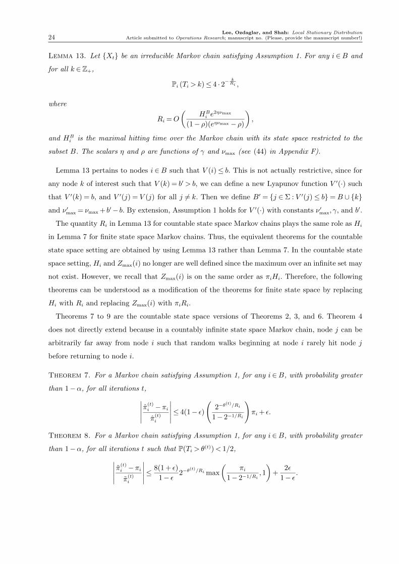
Lemma 13. Let Xt be an irreducible Markov chain satisfying Assumption 1. For any i∈B and
for all k ∈Z+,
Pi (Ti >k)≤ 4 · 2−kRi ,
where
Ri =O
(HBi e
2ηνmax
(1− ρ)(eηνmax − ρ)
),
and HBi is the maximal hitting time over the Markov chain with its state space restricted to the
subset B. The scalars η and ρ are functions of γ and νmax (see (44) in Appendix F).
Lemma 13 pertains to nodes i ∈B such that V (i)≤ b. This is not actually restrictive, since for
any node k of interest such that V (k) = b′ > b, we can define a new Lyapunov function V ′(·) such
that V ′(k) = b, and V ′(j) = V (j) for all j 6= k. Then we define B′ = j ∈ Σ : V ′(j)≤ b=B ∪ k
and ν ′max = νmax + b′− b. By extension, Assumption 1 holds for V ′(·) with constants ν ′max, γ, and b′.
The quantity Ri in Lemma 13 for countable state space Markov chains plays the same role as Hi
in Lemma 7 for finite state space Markov chains. Thus, the equivalent theorems for the countable
state space setting are obtained by using Lemma 13 rather than Lemma 7. In the countable state
space setting, Hi and Zmax(i) no longer are well defined since the maximum over an infinite set may
not exist. However, we recall that Zmax(i) is on the same order as πiHi. Therefore, the following
theorems can be understood as a modification of the theorems for finite state space by replacing
Hi with Ri and replacing Zmax(i) with πiRi.
Theorems 7 to 9 are the countable state space versions of Theorems 2, 3, and 6. Theorem 4
does not directly extend because in a countably infinite state space Markov chain, node j can be
arbitrarily far away from node i such that random walks beginning at node i rarely hit node j
before returning to node i.
Theorem 7. For a Markov chain satisfying Assumption 1, for any i∈B, with probability greater
than 1−α, for all iterations t,∣∣∣∣∣ π(t)i −πiπ
(t)i
∣∣∣∣∣≤ 4(1− ε)
(2−θ
(t)/Ri
1− 2−1/Ri
)πi + ε.
Theorem 8. For a Markov chain satisfying Assumption 1, for any i∈B, with probability greater
than 1−α, for all iterations t such that P(Ti > θ(t))< 1/2,∣∣∣∣∣ π(t)
i −πiπ
(t)i
∣∣∣∣∣≤ 8(1 + ε)
1− ε2−θ
(t)/Ri max
(πi
1− 2−1/Ri,1
)+
2ε
1− ε.
Lee, Ozdaglar, and Shah: Local Stationary DistributionArticle submitted to Operations Research; manuscript no. (Please, provide the manuscript number!) 25
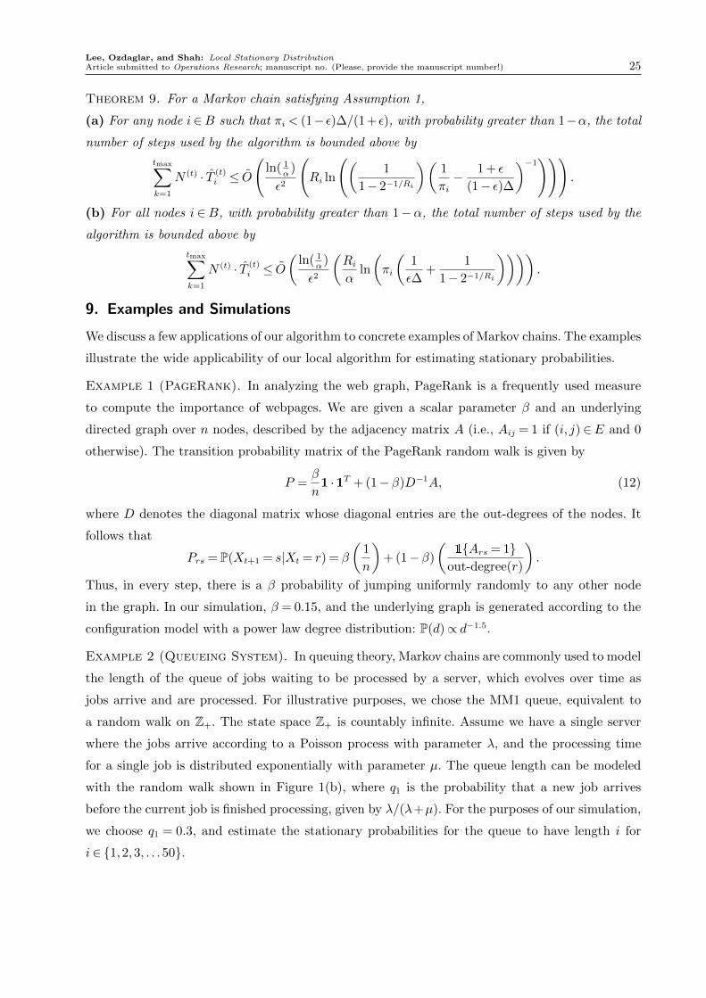
Theorem 9. For a Markov chain satisfying Assumption 1,
(a) For any node i∈B such that πi < (1− ε)∆/(1+ ε), with probability greater than 1−α, the total
number of steps used by the algorithm is bounded above by
tmax∑k=1
N (t) · T (t)i ≤ O
(ln( 1
α)
ε2
(Ri ln
((1
1− 2−1/Ri
)(1
πi− 1 + ε
(1− ε)∆
)−1)))
.
(b) For all nodes i ∈B, with probability greater than 1−α, the total number of steps used by the
algorithm is bounded above by
tmax∑k=1
N (t) · T (t)i ≤ O
(ln( 1
α)
ε2
(Riα
ln
(πi
(1
ε∆+
1
1− 2−1/Ri
)))).
9. Examples and Simulations
We discuss a few applications of our algorithm to concrete examples of Markov chains. The examples
illustrate the wide applicability of our local algorithm for estimating stationary probabilities.
Example 1 (PageRank). In analyzing the web graph, PageRank is a frequently used measure
to compute the importance of webpages. We are given a scalar parameter β and an underlying
directed graph over n nodes, described by the adjacency matrix A (i.e., Aij = 1 if (i, j) ∈E and 0
otherwise). The transition probability matrix of the PageRank random walk is given by
P =β
n1 ·1T + (1−β)D−1A, (12)
where D denotes the diagonal matrix whose diagonal entries are the out-degrees of the nodes. It
follows that
Prs = P(Xt+1 = s|Xt = r) = β
(1
n
)+ (1−β)
(1Ars = 1
out-degree(r)
).
Thus, in every step, there is a β probability of jumping uniformly randomly to any other node
in the graph. In our simulation, β = 0.15, and the underlying graph is generated according to the
configuration model with a power law degree distribution: P(d)∝ d−1.5.
Example 2 (Queueing System). In queuing theory, Markov chains are commonly used to model
the length of the queue of jobs waiting to be processed by a server, which evolves over time as
jobs arrive and are processed. For illustrative purposes, we chose the MM1 queue, equivalent to
a random walk on Z+. The state space Z+ is countably infinite. Assume we have a single server
where the jobs arrive according to a Poisson process with parameter λ, and the processing time
for a single job is distributed exponentially with parameter µ. The queue length can be modeled
with the random walk shown in Figure 1(b), where q1 is the probability that a new job arrives
before the current job is finished processing, given by λ/(λ+µ). For the purposes of our simulation,
we choose q1 = 0.3, and estimate the stationary probabilities for the queue to have length i for
i∈ 1,2,3, . . .50.

Lee, Ozdaglar, and Shah: Local Stationary Distribution26 Article submitted to Operations Research; manuscript no. (Please, provide the manuscript number!)
Example 3 (Magnet Graph). This example illustrates a Markov chain with poor mixing prop-
erties. The Markov chain is depicted in Figure 1(c), and can be described as a random walk over
a finite section of the integers such that there are two attracting states, labeled in Figure 1(c) as
states 1 and n2. We assume that q1, q2 < 1/2, such that for all states left of state n1, the random
walk will drift towards state 1 with probablity 1− q1 in each step, and for all states right of state
n1, the random walk will drift towards state n2 with probability 1− q2 in each step. Due to this
bipolar attraction, a random walk that begins on the left will tend to stay on the left, and similarly,
a random walk that begins on the right will tend to stay on the right. For our simulations, we chose
q1 = q2 = 0.3, n1 = 25, and n2 = 50.
9.1. Algorithm Results for the Anchor Node
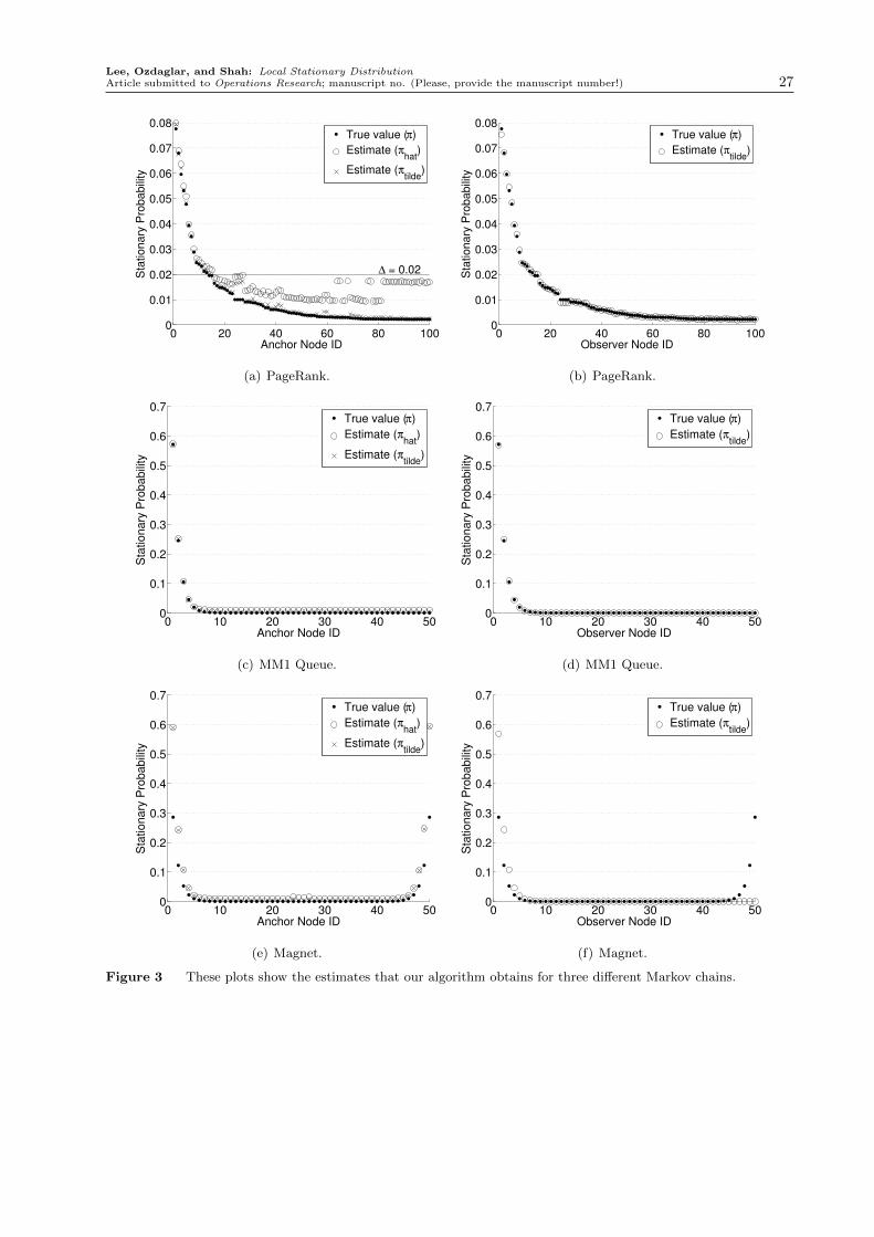
We show the results of applying our algorithm to estimate the stationary probabilities in these
three different Markov chains, using parameters ∆ = 0.02, ε= 0.15, and α= 0.2. Figure 3 plots the
final estimates along with the true stationary probabilities. The three Markov chains have different
mixing properties, chosen to illustrate the performance of our algorithm on Markov chains with
different values of Hi and Zmax(i).
Figures 3(a), 3(c), and 3(e) plot the estimates π(tmax)i and π
(tmax)i for the anchor nodes. Thus,
the data points for different anchor nodes are results from running independent instances of the
algorithm with different nodes chosen as the anchor. In the PageRank Markov chain, we label the
nodes in decreasing order of their true stationary probability πi, since there is no natural ordering
over nodes. In the MM1 queue and the Magnet Markov chains, the nodes are labeled according to
Figures 1(b) and 1(c).
Figure 3(a) shows the result for PageRank. For nodes such that πi > ∆, πi is a close approx-
imation for πi. For nodes such that πi ≤ ∆, the algorithm successfully categorizes the node as
unimportant (i.e. πi ≤∆). In addition, we observe that πi is extremely close to πi for most nodes.
We verify that (Zii−Zqi) is close to 1 for most pairs of nodes (i, q) in the PageRank Markov chain.
Therefore Γi ≈ 1, and Lemmas 9 and 10 indicate that πi is expected to be a closer estimate than
πi, which is consistent with our results.
Figure 3(c) plots the result for the MM1 queue Markov chain. Both estimates πi and πi are close
to πi. Since the stationary probabilities decay exponentially, only the first few nodes are significant,
and the algorithm correctly captures that. Both the PageRank and the MM1 queue Markov chains
mix well, and as expected, our algorithm performs well.
Figure 3(e) shows the result for the Magnet Markov chain, which mixes very slowly. The algo-
rithm overestimates the stationary probabilities by almost two times the true value. This is due to
Lee, Ozdaglar, and Shah: Local Stationary DistributionArticle submitted to Operations Research; manuscript no. (Please, provide the manuscript number!) 27
0 20 40 60 80 1000
0.01
0.02
0.03
0.04
0.05
0.06
0.07
0.08
Anchor Node ID
Sta
tionary
Pro
babili
ty
∆ = 0.02
True value (π)
Estimate (πhat
)
Estimate (πtilde
)
(a) PageRank.
0 20 40 60 80 1000
0.01
0.02
0.03
0.04
0.05
0.06
0.07
0.08
Observer Node ID
Sta
tionary
Pro
babili
ty
True value (π)
Estimate (πtilde
)
(b) PageRank.
0 10 20 30 40 500
0.1
0.2
0.3
0.4
0.5
0.6
0.7
Anchor Node ID
Sta
tio
na
ry P
rob
ab
ility
True value (π)
Estimate (πhat
)
Estimate (πtilde
)
(c) MM1 Queue.
0 10 20 30 40 500
0.1
0.2
0.3
0.4
0.5
0.6
0.7
Observer Node ID
Sta
tio
na
ry P
rob
ab
ility
True value (π)
Estimate (πtilde
)
(d) MM1 Queue.
0 10 20 30 40 500
0.1
0.2
0.3
0.4
0.5
0.6
0.7
Anchor Node ID
Sta
tio
na
ry P
rob
ab
ility
True value (π)
Estimate (πhat
)
Estimate (πtilde
)
(e) Magnet.
0 10 20 30 40 500
0.1
0.2
0.3
0.4
0.5
0.6
0.7
Observer Node ID
Sta
tio
na
ry P
rob
ab
ility
True value (π)
Estimate (πtilde
)
(f) Magnet.
Figure 3 These plots show the estimates that our algorithm obtains for three different Markov chains.

Lee, Ozdaglar, and Shah: Local Stationary Distribution28 Article submitted to Operations Research; manuscript no. (Please, provide the manuscript number!)
0 50 1000
0.2
0.4
0.6
0.8
1
Anchor Node ID
Fra
ctio
n of
sam
ples
trun
cate
d
(a) PageRank: p(tmax)
0 50 10050
100
150
200
250
300
Anchor Node ID
Tru
ncat
ion
thre
shol
d
(b) PageRank: θ(tmax)
0 50 1000
2
4
6x 10⁵
Anchor Node ID
Tot
al n
umbe
r of
ste
ps ta
ken
(c) PageRank: Total Steps
0 20 40 600
0.1
0.2
0.3
0.4
0.5
Anchor Node ID
Fra
ctio
n of
sam
ples
trun
cate
d
(d) MM1 Queue: p(tmax)
0 20 40 600
100
200
300
Anchor Node ID
Tru
ncat
ion
thre
shol
d
(e) MM1 Queue: θ(tmax)
0 20 40 600
2
4
6
8x 10⁵
Anchor Node ID
Tot
al n
umbe
r of
ste
ps ta
ken
(f) MM1 Queue: Total Steps
0 20 40 600
0.2
0.4
0.6
0.8
Anchor Node ID
Fra
ctio
n of
sam
ples
trun
cate
d
(g) Magnet: p(tmax)
0 20 40 600
100
200
300
Anchor Node ID
Tru
ncat
ion
thre
shol
d
(h) Magnet: θ(tmax)
0 20 40 600
2
4
6
8x 10⁵
Anchor Node ID
Tot
al n
umbe
r of
ste
ps ta
ken
(i) Magnet: Total Steps
Figure 4 This shows the value of three variables from the final iteration of the algorithm: fraction of samples
truncated = p(tmax); truncation threshold = θ(tmax); and total number of random walk steps taken =
N (tmax) · T (tmax)i .
the fact that the random samples have close to zero probability of sampling from the opposite half
of the graph. Therefore the estimates are computed without being able to observe the opposite
half of the graph. As the challenge is due to the poor mixing properties of the graph, both πi and
πi are poor estimates. In the figure, it is difficult to distinguish the two estimates because they are
nearly the same and thus superimposed upon each other. We compute the fundamental matrix Z
for this Markov chain, and find that for most pairs i, j ∈Σ, |Zij| is on the order of 109.
Standard methods such as power iteration or MCMC will also perform poorly on this graph, as
it would take an incredibly large amount of time for the random walk to fully mix across the middle

Lee, Ozdaglar, and Shah: Local Stationary DistributionArticle submitted to Operations Research; manuscript no. (Please, provide the manuscript number!) 29
border. The final outputs of both methods are very sensitive to the starting vector, since with high
probability each random walk will stay on the half of the graph in which it was initialized. The
estimates are neither guaranteed to be upper or lower bounds upon the true stationary probability.
Figure 4 plots the quantities p(tmax), θ(tmax), and N (tmax) · T (tmax)i for the execution of our algorithm
on these three examples as a function of the chosen anchor node. We observe a correlation between
these quantities and the stationary probability of a node. Consider the results for the MM1 queue
Markov chain shown in Figures 4(d), 4(e), and 4(f). The fraction of samples truncated, the trunca-
tion threshold, and the total computation time increase as πi decreases, and then flattens out for
nodes i greater than 10. This illustrates the effect of the truncation and termination conditions.
For nodes with small πi, although Ei[Ti] is large, because of the termination condition involving
∆, the algorithm will terminate quickly, not wasting extra time to obtain unnecessary precision.
9.2. Algorithm Results for Observer Nodes
Figures 3(b), 3(d), and 3(f) plot results of a single execution of the algorithm when the anchor
node is fixed to be node 1. The estimates π(tmax)j for a set of observer nodes is plotted along side
the true value for πj. In the PageRank and Magnet Markov chains, J = Σ, and for the MM1 queue
Markov chain, J is the first 50 nodes.
Figures 3(b) and 3(d) both show that the estimates πj are indeed close to πj. As expected, Figure
3(f) shows that the algorithm overestimates the leftmost nodes by a factor of two, and completely
does not detect the nodes on the right. Again, this is due to the poor mixing of the Markov chain
such that the probability of visiting the opposite half of the graph is very small. The severity of
this effect will depend on the choice of q1 and q2. This is a graph on which any local algorithm
will perform poorly on, since the algorithm will not be aware of the second attracting node on the
opposite end.
9.3. Algorithm performance as a function of ∆
Figure 5 shows the results of our algorithm as a function of ∆. Recall that parameter ∆ only
affects the termination conditions of the algorithm. The plot shows results from three separate
executions of the algorithm with different anchor nodes, chosen to illustrate the behavior on nodes
with varying πi. Figures 5(a) and 5(c) plot the estimates for the stationary probability, and Figures
5(b) and 5(d) plot the total steps taken in the last iteration of the algorithm, which we recall is
of the same order as the total random walk steps over all iterations. The figures are shown on a
log-log scale. The results confirm that the computation time of the algorithm is upper bounded by
O(1/∆), which is linear when plotted on log-log scale. When ∆> πi, then πi is effectively lower
bounded at ∆, and the computation time behaves as 1/∆. When ∆ < πi, then πi concentrates
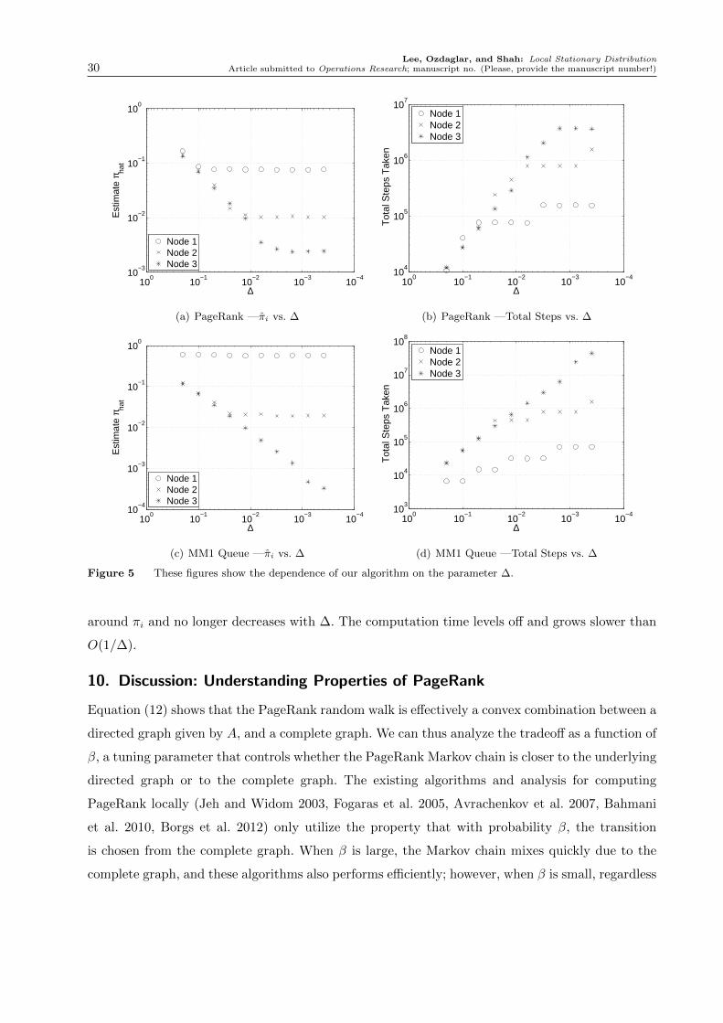
Lee, Ozdaglar, and Shah: Local Stationary Distribution30 Article submitted to Operations Research; manuscript no. (Please, provide the manuscript number!)
10−4
10−3
10−2
10−1
100
10−3
10−2
10−1
100
∆
Est
imat
e π ha
t
Node 1Node 2Node 3
(a) PageRank —πi vs. ∆
10−4
10−3
10−2
10−1
100
104
105
106
107
∆
Tot
al S
teps
Tak
en
Node 1Node 2Node 3
(b) PageRank —Total Steps vs. ∆
10−4
10−3
10−2
10−1
100
10−4
10−3
10−2
10−1
100
∆
Est
imat
e π ha
t
Node 1Node 2Node 3
(c) MM1 Queue —πi vs. ∆
10−4
10−3
10−2
10−1
100
103
104
105
106
107
108
∆
Tot
al S
teps
Tak
en
Node 1Node 2Node 3
(d) MM1 Queue —Total Steps vs. ∆
Figure 5 These figures show the dependence of our algorithm on the parameter ∆.
around πi and no longer decreases with ∆. The computation time levels off and grows slower than
O(1/∆).
10. Discussion: Understanding Properties of PageRank
Equation (12) shows that the PageRank random walk is effectively a convex combination between a
directed graph given by A, and a complete graph. We can thus analyze the tradeoff as a function of
β, a tuning parameter that controls whether the PageRank Markov chain is closer to the underlying
directed graph or to the complete graph. The existing algorithms and analysis for computing
PageRank locally (Jeh and Widom 2003, Fogaras et al. 2005, Avrachenkov et al. 2007, Bahmani
et al. 2010, Borgs et al. 2012) only utilize the property that with probability β, the transition
is chosen from the complete graph. When β is large, the Markov chain mixes quickly due to the
complete graph, and these algorithms also performs efficiently; however, when β is small, regardless

Lee, Ozdaglar, and Shah: Local Stationary DistributionArticle submitted to Operations Research; manuscript no. (Please, provide the manuscript number!) 31
of the properties of the underlying graph, the algorithm scales with 1/β, even though the Markov
chain might still mix quickly depending on the underlying graph.
For the following simulations, we restrict ourselves to the personalized PageRank setting. For a
fixed node x and scalar β, we consider the Markov chain with transition probability matrix P :
P = β1 · eTx + (1−β)D−1A, (13)
where A is the adjacency matrix of the underlying graph, generated according to the configuration
model with a power law degree distribution, and D is a diagonal matrix of the out-degrees. In
every step, there is a probability β of returning to the node x, and probability 1− β of choosing
a neighbor at random (according to the configuration model generated graph). We choose four
different nodes in the graph to be node x, and several different values for β. For each combination
of x and β, we consider the number of random walk steps required to estimate πx in the Markov
chain corresponding to transition probability matrix P . This allows us to compare our algorithm
with the existing PageRank algorithm presented by Fogaras et al. (2005) and Avrachenkov et al.
(2007).
Fogaras’ algorithm takes geometric length random walk samples on the underlying graph given
by matrix A, beginning at node x. Our proposed algorithm samples random walks over P that
begin and end at node x. Sample paths in each of these algorithms can be considered as adjacent
contiguous sections of one long sample path over P , which contains the full information that each
algorithm collects about the graph. We would like to minimize the total number of random walk
steps taken (across all sample paths of various lengths).
In the following simulation, we sample ten long random walks starting at node x having five
million steps each. After every ten thousand steps, we compute the current fraction of visits to node
x out of the total steps taken thus far. This quantity converges to πx as the length goes to infinity.
The percentage error between the estimate and the true πx is averaged over all ten samples. Then
we find the smallest number of steps such that the average error is less than 1%. This is shown in
Figure 6(a) as a function of β for four different chosen nodes x. The expected return time to node
x in each of these settings is shown in Figure 6(b). Both figures are shown on log-log scale.
When β is large, the β jump back to x dominates the random walk, causing the random walk to
behave similarly for different chosen nodes x. In this setting β can be used to determine the required
number of samples to achieve good accuracy. When β is small, the random walk approaches that
of the underlying graph, thus the choice of node x greatly affects the computation. The number of
steps to achieve 1% accuracy does not increase much as β decreases for nodes x that have large πx
in the underlying graph (such as node 1). However, for nodes such that πx is small in the underlying

Lee, Ozdaglar, and Shah: Local Stationary Distribution32 Article submitted to Operations Research; manuscript no. (Please, provide the manuscript number!)
10−6
10−4
10−2
100
104
105
106
107
beta (β) parameter
Num
ber
of s
teps
unt
il <
1%
ave
rage
err
or
Node 1Node 2Node 3Node 4
(a) PageRank —# steps needed vs. β
10−6
10−4
10−2
100
100
101
102
103
beta (β) parameter
Exp
ecte
d re
turn
tim
e to
anc
hor
node
(1/
π i)
Node 1Node 2Node 3Node 4
(b) PageRank —Expected return time vs. β
Figure 6 These figures show the number of random walk steps needed to accurately estimate the stationary
probability of a node, as well as the expected return time to a node in a PageRank Markov chain, for
four different nodes, and as a function of the parameter β.
graph (such as node 4), the required number of steps increases significantly as β decreases. We
observe a relationship between Ex[Tx] and the total amount of computation steps needed for 1%
accuracy. This clearly highlights that in the setting when β is very small, it becomes critical to
consider information from the underlying graph in determining the number of steps to sample.
The existing algorithm only uses the parameter β to govern the number of steps taken for the
algorithm, where the length of a sample random walk scales with 1/β. However, for small β, this
is unnecessarily expensive, as some nodes (such as node 1) do not in fact require the number of
sample steps to increase with 1/β. Our proposed algorithm relies on the expected return time to
node x as the length of each sample path, which adjusts for nodes that have varying importances
in the underlying graph.
11. Conclusion
This paper presents a local algorithm for estimating the stationary probabilities of a subset of nodes
in a Markov chain. The algorithm is a truncated Monte Carlo method, sampling return paths to
the anchor node. The key insight it utilizes is that the stationary probability of a node is inversely
proportional to the expected return time to the node Ei[Ti]. In order to obtain estimates for the
observer nodes j 6= i, it uses the property that the stationary probability πj is equal to the fraction
of expected visits to node j along the return path to node i.
We provide theoretical guarantees for the tightness of approximation and computation time of our
algorithm. We guarantee that the estimate π(tmax)i , is an upper bound for πi with high probability.
For Markov chains that mix well, the estimate will be tight with high probability for nodes such

Lee, Ozdaglar, and Shah: Local Stationary DistributionArticle submitted to Operations Research; manuscript no. (Please, provide the manuscript number!) 33
that πi >∆. The analyses and guarantees rely on the property that for many positive recurrent
countable state space Markov chains, the distribution over return times to a node concentrates
around the mean. We showed that this concentration rate is related to the mixing properties of the
Markov chain. The computation time of the algorithm is upper bounded by O (ln(1/α)/ε3∆) with
high probability. Since the computation time is constant with respect to the Markov chain, this
algorithm is suitable for Markov chains with large state spaces. The algorithm has many practical
benefits. It can be implemented easily in a distributed and parallelized fashion, and it only uses
a constant size neighborhood around the anchor node, upper bounded by 1/∆. The computation
only involves counting and taking an average, thus it is simple and memory efficient.
Appendix A: Proofs of Preliminary Results
The proofs of Lemmas 3 to 6 use the following fact:
Fact 1. If∑t
k=1 xk ≤ 1, then∏t
k=1(1−xk)≥ 1−∑t
k=1 xk.
Proof of Lemma 3. Let At denote the eventT
(t)i ∈ (1± ε)Ei
[T
(t)i
]. Since N (t) is a random
variable due to its dependence on T(t−1)i , the distribution of T
(t)i depends on the value of T
(t−1)i .
Conditioned on the event At−1,
N (t) =
⌈3(1 + ε)θ(t) ln(4θ(t)/α)
T(t−1)i ε2
⌉
≥ 3(1 + ε)θ(t) ln(4θ(t)/α)
(1 + ε)Ei[T (t−1)i ]ε2
=3θ(t) ln(4θ(t)/α)
Ei[T (t−1)i ]ε2
. (14)
Then we apply Chernoff’s bound for independent identically distributed bounded random variables
(cf. Theorem 11), substitute in for N (t), and use the facts that Ei[T (t)i ]≥Ei[T (t−1)
i ] and θ(t) = 2t for
all t, to show that
Pi (¬At|At−1)≤ 2exp
(−ε
2N (t)Ei[T (t)i ]
3θ(t)
)
≤ 2exp
(−Ei[T (t)
i ] ln(4θ(t)/α)
Ei[T (t−1)i ]
)≤ α
2θ(t)≤ α
2t+1. (15)
It can be verified that Pi(¬A1) is similarly upper bounded by α4
using the definition of N (1).
Therefore, by Bayes rule and by the fact that T(t)i is independent from T
(k)i conditioned on T
(t−1)i
for all k < t, we show that
Pi
(t⋂
k=1
Ak
)= Pi (A1)
t∏k=2
Pi (At|At−1)≥t∏
k=1
(1− α
2k+1
). (16)
Lee, Ozdaglar, and Shah: Local Stationary Distribution34 Article submitted to Operations Research; manuscript no. (Please, provide the manuscript number!)
By applying Fact 1, it follows that
Pi
(t⋂
k=1
Ak
)≥ 1−
t∑k=1
α
2k+1= 1− α
2(1− 2−t)≥ 1−α. (17)
Proof of Lemma 4. Let At denote the eventT
(t)i ∈ (1± ε)Ei
[T
(t)i
]. Let Bt denote the event
p(t) ∈ Pi(Ti > θ(t))± ε3
. T
(t)i is independent from p
(t−1)i conditioned on T
(t−1)i . Therefore, it follows
from (15) that
Pi(¬At|At−1 ∩Bt−1)≤ α
2t+1.
By applying Hoeffding’s Inequality for Bernoulli random variables to p(k) and substituting (14),
we show that
Pi (¬Bt|At−1 ∩Bt−1)≤ 2exp
(−2
9ε2N (t)
)≤ 2exp
(−2θ(t) ln(4θ(t)/α)
3Ei[T (t−1)i ]
).
Since Ei[T (t−1)i ]≤ θ(t−1) = θ(t)/2,
Pi (¬Bt|At−1 ∩Bt−1)≤ 2exp
(−4
3ln(4θ(t)/α)
)≤ α
2θ(t)≤ α
2t+1.
By applying the union bound, it follows that
Pi (At ∩Bt|At−1 ∩Bt−1)≥ 1− α
2t. (18)
We can easily verify using the same techniques that
Pi(A1 ∩B1)≥ 1− α2.
Therefore,
Pi
(t⋂
k=1
(Bk ∩Ak)
)≥
t∏k=1
(1− α
2k
).
We use Fact 1 to show that
Pi
(t⋂
k=1
(Bk ∩Ak)
)≥ 1−
t∑k=1
α
2k= 1−α(1− 2−t)≥ 1−α.
Proof of Lemma 5. Recall that t0 is defined such that Pi(Ti > θ(t0)) < 12. Let At denote the
eventT
(t)i ∈ (1± ε)Ei
[T
(t)i
]. Let Bt denote the event
(1− p(t))∈ (1± ε)(1−P(Ti > θ
(t)))
.
Pi
(t⋂
k=t0
Bk
t⋂k=1
Ak
)= Pi
(t⋂
k=t0
(Bk ∩Ak)
∣∣∣∣∣t0−1⋂k=1
Ak
)Pi
(t0−1⋂k=1
Ak
). (19)
Lee, Ozdaglar, and Shah: Local Stationary DistributionArticle submitted to Operations Research; manuscript no. (Please, provide the manuscript number!) 35
T(t)i and p(t) are not independent from T
(t−1)i and p(t−1) due to the dependence of N (t) as a random
variable upon T(t−1)i . However, T
(t)i is independent from p
(t−1)i conditioned on T
(t−1)i . Therefore, it
follows from (15) that
Pi(¬At|At−1 ∩Bt−1)≤ α
2t+1. (20)
By using Chernoff’s bound for Bernoulli random variables and substituting (14), we show that
Pi(¬Bt|At−1 ∩Bt−1)≤ 2exp
(−ε
2N (t)(1−Pi(Ti > θ(t)))
3
)≤ 2exp
(−θ
(t) ln(4θ(t)/α)(1−Pi(Ti > θ(t)))
Ei[T (t−1)i ]
). (21)
By definition, Ei[T (t−1)i ]≤ θ(t−1) = θ(t)/2. Since we are given that Pi(Ti > θ(t))≤ 1
2, then
θ(t)(1−Pi(Ti > θ(t)))
Ei[T (t−1)i ]
≥ 1. (22)
By substituting (22) into (21), it follows that
Pi(¬Bt|At−1 ∩Bt−1)≤ 2α
4θ(t)≤ α
2t+1. (23)
We combine (20) and (23), and apply the union bound to show that
Pi (At ∩Bt|At−1 ∩Bt−1)≥ 1− α
2t. (24)
We can easily verify using the same techniques that
Pi
(At0 ∩Bt0
∣∣∣∣∣t0−1⋂k=1
Ak
)≥ 1− α
2t0.
We use Bayes’ rule and substitute (16) and (24) into (19) to show that
Pi
(t⋂
k=t0
Bk
t⋂k=1
Ak
)≥
t∏k=t0
(1− α
2k
) t0−1∏k=1
(1− α
2k+1
).
We apply Fact 1 to show that
Pi
(t⋂
k=t0
Bk
t⋂k=1
Ak
)≥ 1−
t∑k=1
α
2k+
t0∑k=1
α
2k+1= 1−α(1− 2−t) +
t0∑k=1
α
2k+1≥ 1−α.
Proof of Lemma 6. Let At denote the eventT
(t)i ∈ (1± ε)Ei
[T
(t)i
]. Let Bt denote the event
F(k)j ∈Ei
[F
(k)j
]± εEi
[T
(k)i
]. T
(t)i is independent from F
(t−1)j conditioned on T
(t−1)i . Therefore,
it follows from (15) that
Pi(¬At|At−1 ∩Bt−1)≤ α
2t+1.

Lee, Ozdaglar, and Shah: Local Stationary Distribution36 Article submitted to Operations Research; manuscript no. (Please, provide the manuscript number!)
Recall from the definition of F(t)j that F
(t)j ∈ [0, θ(t)]. Therefore, by applying Chernoff’s bound for
independent identically distributed bounded random variables, and substituting (14), we show that
Pi (¬Bt|At−1 ∩Bt−1)≤ 2exp
−(εEi[T (t)i ]
Ei[F (t)j ]
)2N (t)Ei[F (t)
j ]
3θ(t)
≤ 2exp
(−Ei[T (t)
i ]2 ln(4θ(t)/α)
Ei[F (t)j ]Ei[T (t−1)
i ]
). (25)
Since Ei[T (t)i ]≥Ei[T (t−1)
i ] and Ei[T (t)i ]≥Ei[F (t)
j ], then
Ei[T (t)i ]2
Ei[F (t)j ]Ei[T (t−1)
i ]≥ 1.
By substituting into (25), it follows that
Pi (¬Bt|At−1 ∩Bt−1)≤ 2α
4θ(t)≤ α
2t+1.
By applying the union bound, we show that
Pi (At ∩Bt|At−1 ∩Bt−1)≥ 1− α
2t. (26)
We can easily verify using the same techniques that
Pi(A1 ∩B1)≥ 1− α2.
Therefore,
Pi
(t⋂
k=1
(Bk ∩Ak)
)≥
t∏k=1
(1− α
2k
).
We use the Fact 1 to show that
Pi
(t⋂
k=1
(Bk ∩Ak)
)≥ 1−
t∑k=1
α
2k= 1−α(1− 2−t)≥ 1−α.
Proof of Lemma 7. This proof is adapted from a proof found in Aldous and Fill. It is included
here for completeness.
Pi(Ti >mα) =m−1∏s=0
Pi(Ti > (s+ 1)α | Ti > sα)
=m−1∏s=0
(∑j∈Σ
Pi(Ti > (s+ 1)α | Xsα = j,Ti > sα) Pi(Xsα = j | Ti > sα)
).
By the Markov property,
Pi(Ti >mα) =m−1∏s=0
(∑j∈Σ
Pj(Ti >α) Pi(Xsα = j | Ti > sα)
).

Lee, Ozdaglar, and Shah: Local Stationary DistributionArticle submitted to Operations Research; manuscript no. (Please, provide the manuscript number!) 37
By Markov’s inequality,
Pi(Ti >mα)≤m−1∏s=0
(∑j∈Σ
(Ej[Ti]α
)Pi(Xsα = j | Ti > sα)
)
≤m−1∏s=0
(maxj∈Σ Ej[Ti]
α
)=
(Hi
α
)m.
By choosing α= 2Hi and m= bk/2Hic, it follows that
Pi(Ti >k)≤ Pi(Ti >
⌊k
2Hi
⌋· 2Hi
)≤ 2−bk/2Hic ≤ 2 · 2−k/2Hi .
Appendix B: Proofs for Estimation Error
Proof of Theorem 2. By Lemma 3, with probability greater than 1−α, T(t)i ∈ (1± ε)Ei[T (t)
i ] for
all t. Therefore it follows that with probability greater than 1−α,∣∣∣∣∣1− πi
π(t)i
∣∣∣∣∣≤max
(1− (1− ε)Ei[T
(t)i ]
Ei[Ti], (1 + ε)
Ei[T (t)i ]
Ei[Ti]− 1
)
=εEi[T (t)
i ]
Ei[Ti]+ max
(1− Ei[T (t)
i ]
Ei[Ti],Ei[T (t)
i ]
Ei[Ti]− 1
).
Since Ei[T (t)i ]≤Ei[Ti],∣∣∣∣∣1− πi
π(t)i
∣∣∣∣∣≤ εEi[T (t)i ]
Ei[Ti]+ 1− Ei[T (t)
i ]
Ei[Ti]= (1− ε)
(1− Ei[T (t)
i ]
Ei[Ti]
)+ ε (27)
By multiplying (6) by E[T(t)i ], and by loosely upper bounding (Zii−Zqi) by Zmax(i) for all q, we
obtain
1− Ei[T (t)i ]
Ei[Ti]≤ 2Zmax(i)Pi
(T
(t)i > θ(t)
). (28)
Substitute (28) into (27), and apply Lemma 7 to complete the first statement of the proof. Next,
we need to show that when the algorithm terminates at condition (b), P(Ti > θ)≤ ε( 43
+ε) with high
probability. When the algorithm terminates at condition (b), p(t)π(t)i < ε∆ and π
(t)i ≥ ∆
1+ε. Therefore,
p(t) < ε(1 + ε). By Lemma 4, with probability greater than 1−α, Pi(Ti > θ(t))≤ p(t) + ε3≤ ε( 4
3+ ε).
Therefore, it follows that∣∣∣∣∣ π(t)i −πiπ
(t)i
∣∣∣∣∣≤ 2ε(1− ε)(
4
3+ ε
)Zmax(i) + ε≤ ε (3Zmax(i) + 1) .

Lee, Ozdaglar, and Shah: Local Stationary Distribution38 Article submitted to Operations Research; manuscript no. (Please, provide the manuscript number!)
Proof of Theorem 3. By Lemma 5, with probability greater than 1−α, T(t)i ∈ (1± ε)Ei[T (t)
i ] for
all t, and (1− p(t)) ∈ (1± ε)(1− Pi(Ti > θ(t))) for all t such that Pi(Ti > θ(t))> 12. Therefore, with
probability greater than 1−α, for every t such that Pi(Ti > θ(t))> 12,∣∣∣∣∣1− T
(t)i
(1− p(t))Ei[Ti]
∣∣∣∣∣≤max
(1− (1− ε)Ei[T (t)
i ]
(1 + ε)(1−Pi(Ti > θ(t)))Ei[Ti],
(1 + ε)Ei[T (t)i ]
(1− ε)(1−Pi(Ti > θ(t)))Ei[Ti]− 1
)
≤max
(1− ε1 + ε
(1− Ei[T (t)
i ]
(1−Pi(Ti > θ(t)))Ei[Ti]
),1 + ε
1− ε
(Ei[T (t)
i ]
(1−Pi(Ti > θ(t)))Ei[Ti]− 1
))+
2ε
1− ε
≤ 1 + ε
1− ε
∣∣∣∣∣1− Ei[T (t)i ]
(1−Pi(Ti > θ(t)))Ei[Ti]
∣∣∣∣∣+ 2ε
1− ε. (29)
By rearranging (10), and upper bounding (Zii−Zqi) by Zmax(i) for all q, it follows that∣∣∣∣∣1− Ei[T (t)i ]
(1−Pi(Ti > θ(t)))Ei[Ti]
∣∣∣∣∣≤max(2Zmax(i)− 1,1)
Pi(T
(t)i > θ(t)
)1−Pi
(T
(t)i > θ(t)
) . (30)
Substitute (30) into (29), and apply Lemma 7 to complete the proof.
In order to analyze the distribution over the number of visits to node j on a return path to node
i, we will use the following Lemma as stated by Aldous and Fill (1999).
Lemma 14 (Aldous, Fill). For distinct i, k ∈Σ, the expected number of visits to a node j begin-
ning from node k before visiting i is equal to
Ek
[∞∑t=1
1Xt = j1t≤ Ti
]= πj(Ek[Ti] +Ei[Tj]−Ek[Tj]).
Proof of Lemma 11. By definition,
Ei[Fj]−Ei[F (t)j ]
=Ei
[∞∑t=1
1Xt = j1t≤ Ti
]−Ei
θ(t)∑t=1
1Xt = j1t≤ Ti
= P
(Ti > θ
(t))Ei
∞∑t=θ(t)
1Xt = j1t≤ Ti
∣∣∣∣∣∣Ti > θ(t)
= P
(Ti > θ
(t)) ∑q∈Σ\i
Pi(Xθ(t) = q|Ti > θ(t)
)Ei
∞∑t=θ(t)+1
1Xt = j1t≤ Ti
∣∣∣∣∣∣Xθ(t) = q,Ti > θ(t)
= P
(Ti > θ
(t)) ∑q∈Σ\i
Pi(Xθ(t) = q|Ti > θ(t)
)Eq
[∞∑t=1
1Xt = j1t≤ Ti
].

Lee, Ozdaglar, and Shah: Local Stationary DistributionArticle submitted to Operations Research; manuscript no. (Please, provide the manuscript number!) 39
We divide by Ei[Fj] and use Lemma 14 and Lemma 1(a) to show that
1−Ei[F (t)
j ]
Ei[Fj]
=P(Ti > θ
(t))
Ei[Fj]∑
q∈Σ\i
Pi(Xθ(t) = q|Ti > θ(t)
)πj(Eq[Ti] +Ei[Tj]−Eq[Tj])
= P(Ti > θ
(t)) ∑q∈Σ\i
Pi(Xθ(t) = q|Ti > θ(t)
) (Eq[Ti] +Ei[Tj]−Eq[Tj])Ei[Ti]
. (31)
By multiplying (9) by Ei[T (t)i ], it follows that
1− Ei[T (t)i ]
Ei[Ti]= Pi
(Ti > θ
(t)) ∑q∈Σ\i
Pi(Xθ(t) = q|Ti > θ(t)
) Eq[Ti]Ei[Ti]
. (32)
We use (31) and (32))= to show that
Ei[F (t)j ]
Ei[T (t)i ]−πj =
Ei[Fj]Ei[T (t)
i ]
(Ei[F (t)
j ]
Ei[Fj]− Ei[T (t)
i ]
Ei[Ti]
)
=Ei[Fj]Ei[T (t)
i ]P(Ti > θ
(t)) ∑q∈Σ\i
Pi(Xθ(t) = q|Ti > θ(t)
) (Eq[Tj]−Ei[Tj])Ei[Ti]
=P(Ti > θ
(t))
Ei[T (t)i ]
∑q∈Σ\i
Pi(Xθ(t) = q|Ti > θ(t)
)πj(Eq[Tj]−Ei[Tj]).
By Lemma 2,
Ei[F (t)j ]
Ei[Ti]−πj =
P(Ti > θ
(t))
Ei[T (t)i ]
∑q∈Σ\i
Pi(Xθ(t) = q|Ti > θ(t)
)(Zij −Zqj)
.
Proof of Theorem 4. By Lemma 6, with probability greater than 1−α, F(t)j ∈Ei[F
(t)j ]±εEi[T (t)
i ]
and T(t)i ∈ (1± ε)Ei[T (t)
i ] for all t. Therefore with probability greater than 1−α,
(1− ε)F (t)j
T(t)i
≤Ei[F (t)
j ] + εEi[T (t)i ]
Ei[T (t)i ]
.
Therefore,
π(t)j ≤
Ei[F (t)j ]
Ei[T (t)i ]
+ ε+ επ(t)j .
Similarly,
(1 + ε)F(t)j
T(t)i
≥Ei[F (t)
j ]− εEi[T (t)i ]
Ei[T (t)i ]
π(t)j ≥
Ei[F (t)j ]
Ei[T (t)i ]− ε− επ(t)
j .

Lee, Ozdaglar, and Shah: Local Stationary Distribution40 Article submitted to Operations Research; manuscript no. (Please, provide the manuscript number!)
Therefore, with probability greater than 1−α,∣∣∣π(t)j −πj
∣∣∣≤max
(Ei[F (t)
j ]
Ei[T (t)i ]
+ ε(1 + π(t)j )−πj, πj −
Ei[F (t)j ]
Ei[T (t)i ]
+ ε(1 + π(t)j )
)
=
∣∣∣∣∣Ei[F(t)j ]
Ei[T (t)i ]−πj
∣∣∣∣∣+ ε(1 + π(t)j ).
Use Lemma 11 to show that with probability greater than 1−α,∣∣∣π(t)j −πj
∣∣∣≤∣∣∣∣∣∣P(Ti > θ
(t))
Ei[T (t)i ]
∑k∈Σ\i
Pi(Xθ(t) = k|Ti > θ(t)
)Zij −Zkj
∣∣∣∣∣∣+ ε(1 + π(t)j )
≤P(Ti > θ
(t))
Ei[T (t)i ]
2Zmax(j) + ε(1 + π(t)j ).
Since T(t)i ∈ (1± ε)Ei[T (t)
i ], it follows that∣∣∣π(t)j −πj
∣∣∣≤ (1 + ε)P(Ti > θ
(t))
2Zmax(j)π(t)i + ε(1 + π
(t)j ).
Apply Lemma 7 to complete the proof.
Appendix C: Proofs for Computation Time
Proof of Theorem 6(a). Let t be large enough such that
θ(t) = 2t ≥ 2Hi
ln 2ln
((2
1− 2−1/2Hi
)(1
πi− (1 + ε)
(1− ε)∆
)−1). (33)
Since we are given that πi <(1−ε)∆(1+ε)
, this expression is well defined.W e apply Lemma 7 to Lemma
8 to show
Ei[Ti]−Ei[T (t)i ]≤
∞∑k=θ(t)
2 · 2−k/2Hi =2 · 2−θ(t)/2Hi1− 2−1/2Hi
. (34)
By substituting (33) into (34), it follows that
Ei[T (t)i ]≥Ei[Ti]−
(1
πi− (1 + ε)
(1− ε)∆
)=
(1 + ε)
(1− ε)∆. (35)
By combining Lemma 3 and (33), with probability greater than 1−α,
π(t)i =
1
T(t)i
≤ 1
(1− ε)Ei[T (t)i ]
,
≤ ∆
(1 + ε),
satisfying termination condition (a). Therefore, with probability greater than 1−α, the number of
iterations in the algorithm is bounded above by
tmax ≤ ln
(2Hi
ln 2ln
((2
1− 2−1/2Hi
)(1
πi− (1 + ε)
(1− ε)∆
)−1))
.
Combine this with Lemma 12 to finish the proof.

Lee, Ozdaglar, and Shah: Local Stationary DistributionArticle submitted to Operations Research; manuscript no. (Please, provide the manuscript number!) 41
Proof of Theorem 6(b). Let t be large enough such that
θ(t) = 2t ≥ 2Hi
ln 2ln
(2πi
(2
(1− ε)ε∆+
1
1− 2−1/2Hi
)). (36)
By substituting (36) into Lemma 7, it follows that
Pi(Ti > θ
(t))≤Ei[Ti]
(2
(1− ε)ε∆+
1
1− 2−1/2Hi
)−1
. (37)
Substitute (36) into (34) to show that
Ei[T (t)i ]≥Ei[Ti]−Ei[Ti]
(2
(1− ε)ε∆+
1
1− 2−1/2Hi
)−1 (1− 2−1/Hi
)−1. (38)
We combine (37) and (38) to show that
Pi(Ti > θ
(t))
Ei[T (t)i ]
≤ 1(2
(1−ε)ε∆ + 1
1−2−1/2Hi
)− (1− 2−1/2Hi)
−1=
(1− ε)ε∆2
. (39)
By applying (17) to (39), it follows that with probability greater than 1− α2,
Pi(Ti > θ
(t))π
(t)i =
Pi(Ti > θ
(t))
T(t)i
≤Pi(Ti > θ
(t))
(1− ε)Ei[T (t)i ]≤ ε∆
2.
By Markov’s inequality, for each time t,
P(p(t) ≤ 2Pi(Ti > θ(t))
)≥ 1
2.
Therefore, with probability greater than 12,
p(t)π(t)i ≤ 2Pi
(Ti > θ
(t))π
(t)i ≤ ε∆,
and the algorithm will satisfy termination condition (b). If the algorithm does not terminate in
this iteration, then the algorithm will terminate in the next iteration with probability greater than
12. Thus after another additional log2( 2
α) iterations, we can guarantee that with probability greater
than 1− α2, the algorithm will terminate. We apply the union bound to show that since θ(t) = 2t,
with probability greater than 1− α, the number of iterations needed in the algorithm is upper
bounded by
t≤ log2(2/α) + log2
(2Hi
ln 2ln
(2πi
(2
(1− ε)ε∆+
1
1− 2−1/2Hi
)))= log2
(4Hi
α ln 2ln
(2πi
(2
(1− ε)ε∆+
1
1− 2−1/2Hi
)))

Lee, Ozdaglar, and Shah: Local Stationary Distribution42 Article submitted to Operations Research; manuscript no. (Please, provide the manuscript number!)
Appendix D: Proofs for Countable State Space Markov Chains
To prove that the return times concentrate for countably infinite state space Markov chains, we
use Lyapunov function analysis introduced by Foster (1953). We establish that indeed return times
have exponentially decaying tail even for countable-state space Markov chain as long as they satisfy
Assumption 1.
Useful notation. We introduce formal notation for observing Xtt≥0 over the subset B. Let
Ytt≥0 be a Markov chain with state space B. Yt is a subsequence of Xt constructed in the
following way. Define the subsequence Sk of Z+ as:
S0 , 0, Sk ,mint > Sk−1 :Xt ∈B,
and define Yt ,XSt such that
PY (x, y) = P (XS1 = y|X0 = x) for any x, y ∈B.
Let Qt , St+1−St, the length of the path between XSt and XSt+1.
Let TBi , inft≥ 1 | Yt = i, the return time to i for the chain Yt.Let HB
i ,maxj∈B Ej [TBi ], the maximal expected hitting time to node i for the chain Yt. We can
use these variables to express the return time to node i by
Ti = STBi=
TBi −1∑k=0
Qk. (40)
Lemma 15. Let Xt be a countable state space Markov chain satisfying Assumption 1. Let Ytbe defined above as the Markov chain restricted to B, and let Qk be the length between visits to B.
For any W ∈Z+, Z ≥W , and i∈B,
Pi
(W−1∑k=0
Qk >Z
)≤ exp
(0.8(1− ρ)
eηνmax
(1.25We2ηνmax
(1− ρ)(eηνmax − ρ)+W −Z
)).
The constants γ and νmax are given by the Assumption 1, and the scalars η and ρ are functions of
γ and νmax, as defined in (44) in Appendix F.
Proof of Lemma 15. By the law of iterated expectation,
Ei
[W−1∏k=0
exp (λQk)
]=Ei
[exp (λQ0)Ei
[W−1∏k=1
exp (λQk)
∣∣∣∣∣Q0
]]Conditioned on Y1 = j, Y0 and Q0 are independent of Qkk>0, because Y1 = XQ0
. Thus by the
strong Markov property,
Ei
[W−1∏k=1
exp (λQk)
∣∣∣∣∣Q0
]≤max
j∈BE
[W−1∏k=1
exp (λQk)
∣∣∣∣∣Y1 = j
],

Lee, Ozdaglar, and Shah: Local Stationary DistributionArticle submitted to Operations Research; manuscript no. (Please, provide the manuscript number!) 43
so that
Ei
[W−1∏k=0
exp (λQk)
]≤Ei[exp(λQ0)]max
j∈BE
[W−1∏k=1
exp (λQk)
∣∣∣∣∣Y1 = j
].
We iteratively apply conditioning to show that
Ei
[W−1∏k=0
exp (λQk)
]≤Ei[exp(λQ0)]
W−1∏k=1
(maxj∈B
E [ exp (λQk)|Yk = j]
).
We can upper bound Qk by assuming that it always goes on an excursion from B, such that
Qk ≤ 1 + (length of an excursion into Bc).
We invoke Hajek’s result of Theorem 13, with V (x)< b+ νmax to bound the exponential moments
of the excursion. For any i∈B,
Ei
[W−1∏k=0
exp (λQk)
]≤(eλ(eηνmax
(eλ− 1
1− ρeλ
)+ 1
))W,
where η and ρ are functions of γ and νmax, as defined in (44) in Appendix F. They satisfy the
conditions given in Hajek (1982). For λ<min(
0.43, 0.8(1−ρ)ρ
),
eλ < 1 + 1.25λ and 1− ρeλ > 1− ρ− 1.25ρλ.
By substituting in these approximations and using 1 +x< ex, we obtain(eλ(eηνmax
(eλ− 1
1− ρeλ
)+ 1
))W<
(eλ(eηνmax
(1.25λ
1− ρ− 1.25ρλ
)+ 1
))W< exp (λW ) exp
(1.25λWeηνmax
1− ρ− 1.25ρλ
)< exp
(λW
(1.25eηνmax
1− ρ− 1.25ρλ+ 1
)).
By Markov’s inequality,
Pi
(W−1∑k=0
Qk >Z
)≤
Ei[exp
(λ∑W−1
k=0 Qk
)]exp(λZ)
≤ exp
(λW
(1.25eηνmax
1− ρ− 1.25ρλ+ 1
)−λZ
).
Choose λ = 0.8(1−ρ)eηνmax . We can verify that for our choice of η and ρ according to (44), λ <
max(
0.43, 0.8(1−ρ)ρ
)always holds. Therefore, we complete the proof by substituting in for λ,
Pi
(W−1∑k=0
Qk >Z
)≤ exp
(0.8(1− ρ)
eηνmax
(1.25We2ηνmax
(1− ρ)(eηνmax − ρ)+W −Z
)).
Lee, Ozdaglar, and Shah: Local Stationary Distribution44 Article submitted to Operations Research; manuscript no. (Please, provide the manuscript number!)
Proof of Lemma 13. By (40), for any constants W,Z ∈Z+,
TBi ≤W⋂
W−1∑k=0
Qk ≤Z
=⇒ Ti ≤Z.
We use the union bound on the contrapositive statement to obtain the inequalities
Pi(Ti >Z)≤ Pi
(TBi >W∪
W−1∑k=0
Qk >Z
)
≤ Pi(TBi >W ) +Pi
(W−1∑k=0
Qk >Z
). (41)
Choose W = 2HBi
(2 + k
Ri
)and
Z = 4HBi
(1.25e2ηνmax
(1− ρ)(eηνmax − ρ)+ 1
)+
ln(2)eηνmax
0.8(1− ρ)+ k= 2Ri−
ln(2)eηνmax
0.8(1− ρ)+ k.
The next inequality follows from substituting these expressions for W and Z into (41), and applying
Lemmas 7 and 15:
Pi(Ti > 2Ri−
ln(2)eηνmax
0.8(1− ρ)+ k
)≤ 2
− kRi ,
Pi (Ti > 2Ri + k)≤ Pi(Ti > 2Ri−
ln(2)eηνmax
0.8(1− ρ)+ k
)≤ 2
− kRi ,
Pi (Ti >k)≤ 2− k−2Ri
Ri ≤ 4 · 2−kRi .
Proof of Theorem 7. This proof follows a similar proof of Theorem 2. Substitute Lemma 13
into (8) to show that
1− Ei[T (t)i ]
Ei[Ti]=
1
Ei[Ti]
∞∑k=θ(t)
Pi(Ti >k)≤ πi
(4 · 2−θ(t)/Ri1− 2−1/Ri
). (42)
Substitute (42) into (27) to complete the proof.
Proof of Theorem 8. This proof follows a similar proof of Theorem 3. By dividing (8) by (1−
Pi(Ti > θ(t))), it follows that∣∣∣∣∣1− Ei[T (t)i ]
(1−Pi(Ti > θ(t)))Ei[Ti]
∣∣∣∣∣=∣∣∣∣∣∣ 1
(1−Pi(Ti > θ(t)))
πi ∞∑k=θ(t)
Pi(Ti >k)−Pi(Ti > θ(t))
∣∣∣∣∣∣≤ 1
(1−Pi(Ti > θ(t)))max
πi ∞∑k=θ(t)
Pi(Ti >k),Pi(Ti > θ(t))
.

Lee, Ozdaglar, and Shah: Local Stationary DistributionArticle submitted to Operations Research; manuscript no. (Please, provide the manuscript number!) 45
Then we apply Lemma 13 and use the fact that Pi(Ti > θ(t))< 12
to show that∣∣∣∣∣1− Ei[T (t)i ]
(1−Pi(Ti > θ(t)))Ei[Ti]
∣∣∣∣∣≤ 2max
(πi
(4 · 2−θ(t)/Ri1− 2−1/Ri
),4 · 2−θ
(t)/Ri
)
= 8 · 2−θ(t)/Ri max
(πi
1− 2−1/Ri,1
). (43)
Substitute (43) into (29) to complete the proof.
Proof of Theorem 9. The proof is exactly the same as the proof of Theorem 6, except that we
use Lemma 13 rather than Lemma 7.
Appendix E: Chernoff Bounds
Theorem 10 (Chernoff’s Multiplicative Bound for Binomials).
Let X1,X2,X3, . . .XN be a sequence of independent identically distributed Bernoulli random vari-
ables, such that for all i, Xi = 1 with probability p and Xi = 0 otherwise. Then for any ε > 0,
P
(∣∣∣∣∣ 1
N
N∑i=1
Xi−E[X]
∣∣∣∣∣≥ εE[X]
)≤ 2e−
ε2Np3 .
Theorem 11 (Chernoff’s Multiplicative Bound for Bounded Variables).
Let X1,X2,X3, . . .XN be a sequence of independent identically distributed strictly bounded non-
negative random variables, such that Xi ∼X for all i, and X ∈ [0, θ]. Then for any ε > 0,
P
(∣∣∣∣∣ 1
N
N∑i=1
Xi−E[X]
∣∣∣∣∣≥ εE[X]
)≤ 2e−
ε2NE[X]3θ .
Appendix F: Lyapunov Function Analysis
Theorem 12 (Foster 1953). Let Xt be a discrete time, irreducible Markov chain on countable
state space Σ with transition probability matrix P . Xt is positive recurrent if and only if there
exists a Lyapunov function V : Σ→R+, γ > 0 and b≥ 0, such that
1. For all x∈Σ,
E [V (Xt+1)|Xt = x]≤∞,
2. For all x∈Σ such that V (x)> b,
E [V (Xt+1)−V (Xt)|Xt = x]≤−γ.
In words, given a positive recurrent Markov chain, there exists a Lyapunov function V : Σ→R+
and a decomposition of the state space into B = x ∈ Σ : V (x) ≤ b and Bc = x ∈ Σ : V (x) > b
such that there is a uniform negative drift in Bc towards B and |B| is finite.
For any irreducible, Markov chain, the following function is a valid Lyapunov function for γ = 1
and b= 0.5: Choose any node i∈Σ, and fix this as the “central node”. Define the function V : Σ→
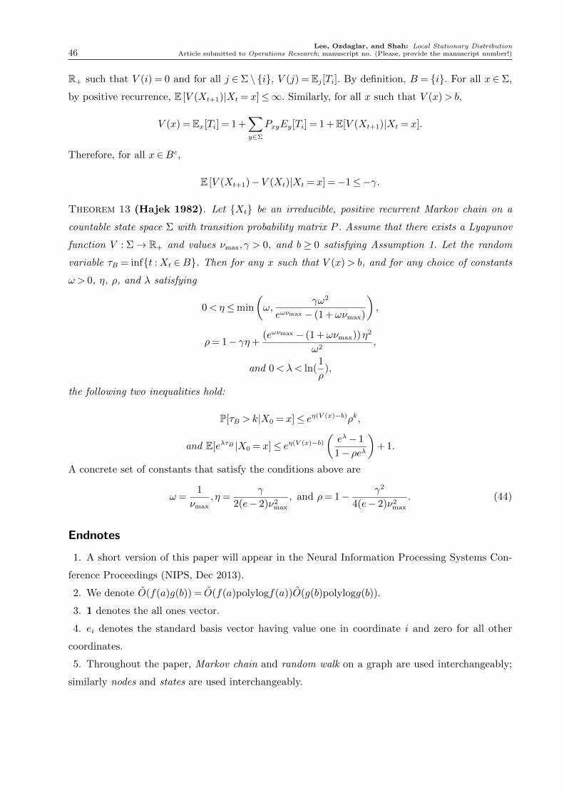
Lee, Ozdaglar, and Shah: Local Stationary Distribution46 Article submitted to Operations Research; manuscript no. (Please, provide the manuscript number!)
R+ such that V (i) = 0 and for all j ∈Σ \ i, V (j) = Ej[Ti]. By definition, B = i. For all x ∈Σ,
by positive recurrence, E [V (Xt+1)|Xt = x]≤∞. Similarly, for all x such that V (x)> b,
V (x) =Ex[Ti] = 1 +∑y∈Σ
PxyEy[Ti] = 1 +E[V (Xt+1)|Xt = x].
Therefore, for all x∈Bc,
E [V (Xt+1)−V (Xt)|Xt = x] =−1≤−γ.
Theorem 13 (Hajek 1982). Let Xt be an irreducible, positive recurrent Markov chain on a
countable state space Σ with transition probability matrix P . Assume that there exists a Lyapunov
function V : Σ→ R+ and values νmax, γ > 0, and b ≥ 0 satisfying Assumption 1. Let the random
variable τB = inft :Xt ∈B. Then for any x such that V (x)> b, and for any choice of constants
ω > 0, η, ρ, and λ satisfying
0< η≤min
(ω,
γω2
eωνmax − (1 +ωνmax)
),
ρ= 1− γη+(eωνmax − (1 +ωνmax))η2
ω2,
and 0<λ< ln(1
ρ),
the following two inequalities hold:
P[τB >k|X0 = x]≤ eη(V (x)−b)ρk,
and E[eλτB |X0 = x]≤ eη(V (x)−b)(eλ− 1
1− ρeλ
)+ 1.
A concrete set of constants that satisfy the conditions above are
ω=1
νmax
, η=γ
2(e− 2)ν2max
, and ρ= 1− γ2
4(e− 2)ν2max
. (44)
Endnotes
1. A short version of this paper will appear in the Neural Information Processing Systems Con-
ference Proceedings (NIPS, Dec 2013).
2. We denote O(f(a)g(b)) = O(f(a)polylogf(a))O(g(b)polylogg(b)).
3. 1 denotes the all ones vector.
4. ei denotes the standard basis vector having value one in coordinate i and zero for all other
coordinates.
5. Throughout the paper, Markov chain and random walk on a graph are used interchangeably;
similarly nodes and states are used interchangeably.

Lee, Ozdaglar, and Shah: Local Stationary DistributionArticle submitted to Operations Research; manuscript no. (Please, provide the manuscript number!) 47
6. A Markov chain is irreducible if and only if the corresponding Markov chain graph is strongly
connected, i.e. for all x, y ∈Σ, there exists a path from x to y.
7. A Markov chain is positive recurrent if the expected time for a random walk beginning at node
i to return to node i is finite. This means that the random walk cannot “drift to infinity”. This is
true for all irreducible finite state space Markov chains.
8. In this example, even if we did not limit the algorithm to using a local neighborhood of i, the
probability that a random walk beginning at node 1 reaches node n1 before returning to state 1 is
very small, decaying exponentially in n1. Therefore, we would need an exponential in n1 number
of samples in order for there to be a reasonable probability that one of the sample random walks
explored the region past node n1. This presents another fundamental limitation of computing
stationary distributions for Markov chains that are not well connected.
Acknowledgments
This work is supported in parts by ARO under MURI awards 58153-MA-MUR and W911NF-11-1-0036, and
grant 56549-NS, and by NSF under grant CIF 1217043 and a Graduate Fellowship.
References
Aldous, D., J. Fill. 1999. Reversible Markov chains and random walks on graphs: Chapter 2 (General Markov
chains). book in preparation. URL: http:// www.stat.berkeley.edu/ ∼aldous/ RWG/ Chap2.pdf 7, 19–20.
Andersen, R., C. Borgs, J. Chayes, J. Hopcraft, V.S. Mirrokni, S.H. Teng. 2007. Local computation of
PageRank contributions. Proceedings of the 5th international conference on Algorithms and models for
the web-graph. WAW’07, Springer-Verlag, Berlin, Heidelberg, 150–165.
Assmussen, S., P. Glynn. 2010. Stochastic Simulation: Algorithms and Analysis (Stochastic Modeling and
Applied Probability). Springer.
Avrachenkov, K., N. Litvak, D. Nemirovsky, N. Osipova. 2007. Monte Carlo methods in PageRank compu-
tation: When one iteration is sufficient. SIAM Journal on Numerical Analysis 45(2) 890–904.
Bahmani, B., A. Chowdhury, A. Goel. 2010. Fast incremental and personalized PageRank. Proc. VLDB
Endow. 4(3) 173–184.
Bertsimas, D., D. Gamarnik, J.N. Tsitsiklis. 1998. Geometric bounds for stationary distributions of infinite
Markov chains via Lyapunov functions. Tech. rep., MIT Sloan School of Management.
Borgs, C., M. Brautbar, J. Chayes, S.H. Teng. 2012. Sublinear time algorithm for PageRank computations
and related applications. CoRR abs/1202.2771.
Candogan, O., K. Bimpikis, A. Ozdaglar. 2012. Optimal pricing in networks with externalities. Operations
Research 60(4) 883–905.
Chasparis, G.C., J.S. Shamma. 2010. Control of preferences in social networks. CDC . 6651–6656.

Lee, Ozdaglar, and Shah: Local Stationary Distribution48 Article submitted to Operations Research; manuscript no. (Please, provide the manuscript number!)
Chen, Y.Y., Q. Gan, T. Suel. 2004. Local methods for estimating PageRank values. Proceedings of the
thirteenth ACM international conference on Information and knowledge management . ACM, 381–389.
Cipra, B. 2000. The best of the 20th century: Editors name top 10 algorithms. SIAM News 33(4) 1.
Diaconis, P. 2009. The Markov chain Monte Carlo revolution. Bulletin of the American Mathematical Society
46(2) 179–205.
Diaconis, P., L. Saloff-Coste. 1998. What do we know about the Metropolis algorithm? Journal of Computer
and System Sciences 57(1) 20–36.
Fogaras, D., B. Racz, K. Csalogany, T. Sarlos. 2005. Towards scaling fully personalized PageRank: Algo-
rithms, lower bounds, and experiments. Internet Mathematics 2(3) 333–358.
Golub, G.H., C.F. Van Loan. 1996. Matrix Computations. Johns Hopkins Studies in the Mathematical
Sciences, Johns Hopkins University Press.
Hajek, B. 1982. Hitting-time and occupation-time bounds implied by drift analysis with applications.
Advances in Applied probability 502–525.
Hastings, W.K. 1970. Monte Carlo sampling methods using Markov chains and their applications. Biometrika
57(1) 97–109.
Haveliwala, T.H. 2003. Topic-sensitive PageRank: A context-sensitive ranking algorithm for web search.
Technical Report 2003-29, Stanford InfoLab. Extended version of the WWW 2002 paper on Topic-
Sensitive PageRank.
Jeh, G., J. Widom. 2003. Scaling personalized web search. Proceedings of the 12th international conference
on World Wide Web. New York, NY, USA, 271–279.
Kamvar, S., T. Haveliwala, C. Manning, G. Golub. 2003. Exploiting the block structure of the web for
computing PageRank. Stanford University Technical Report .
Koury, J.R., D.F. McAllister, W.J. Stewart. 1984. Iterative methods for computing stationary distributions
of nearly completely decomposable Markov chains. SIAM Journal on Algebraic Discrete Methods 5(2)
164–186.
Levin, D.A., Y. Peres, E.L. Wilmer. 2009. Markov chains and mixing times. Amer Mathematical Society.
Metropolis, N., A.W. Rosenbluth, M.N. Rosenbluth, A.H. Teller, E. Teller. 1953. Equation of state calcula-
tions by fast computing machines. The Journal of Chemical Physics 21 1087.
Meyn, S.P., R.L. Tweedie. 1993. Markov chains and stochastic stability . Springer-Verlag.
Negahban, S., S. Oh, D. Shah. 2012. Iterative ranking from pair-wise comparisons. CoRR abs/1209.1688.
Newman, M. E. J. 2010. Networks: an introduction. Oxford University Press, Oxford; New York.
Page, L., S. Brin, R. Motwani, T. Winograd. 1999. The PageRank citation ranking: Bringing order to the
web. Technical Report 1999-66.

Lee, Ozdaglar, and Shah: Local Stationary DistributionArticle submitted to Operations Research; manuscript no. (Please, provide the manuscript number!) 49
Sarma, A. Das, S. Gollapudi, R. Panigrahy. 2011. Estimating PageRank on graph streams. Journal of ACM
58(3) 13.
Sarma, A. Das, A.R. Molla, G. Pandurangan, E. Upfal. 2012. Fast distributed PageRank computation.
CoRR abs/1208.3071.
Semkow, T.M., S. Pomm, S. Jerome, D.J. Strom, eds. 2006. Applied Modeling and Computations in Nuclear
Science. American Chemical Society, Washington, DC.
Shah, D., T. Zaman. 2011. Rumors in a network: Who’s the culprit? IEEE Transactions on Information
Theory 57(8) 5163 –5181.
Stewart, W.J. 1994. Introduction to the numerical solution of Markov chains, vol. 41. Princeton University
Press Princeton.