Computing the Partition Function of the Sherrington ...
97
Computing the Partition Function of the Sherrington-Kirkpatrick Model is Hard on Average Eren C. Kızılda˘ g, joint work with David Gamarnik MIT 2020 IEEE International Symposium on Information Theory June, 2020 D. Gamarnik, E. C. Kızılda˘ g (MIT) Average-Case Hardness of SK Model June, 2020 1 / 22
Transcript of Computing the Partition Function of the Sherrington ...

Computing the Partition Function of the Sherrington-KirkpatrickModel is Hard on Average
Eren C. Kızıldag, joint work with David Gamarnik
MIT
2020 IEEE International Symposium on Information Theory
June, 2020
D. Gamarnik, E. C. Kızıldag (MIT) Average-Case Hardness of SK Model June, 2020 1 / 22

Model and Algorithmic Problem
Overview
1 Model and Algorithmic Problem
2 Part I: Hardness under Finite Precision Arithmetic.Cuts/PolaritiesTruncationMain ResultProof Sketch
3 Part II: Hardness under Real-Valued Model.Setup and ModelMain Result
4 Concluding RemarksExtensionsLimitations and Open Problems
D. Gamarnik, E. C. Kızıldag (MIT) Average-Case Hardness of SK Model June, 2020 2 / 22

Model and Algorithmic Problem
Computing the partition function of the SK model
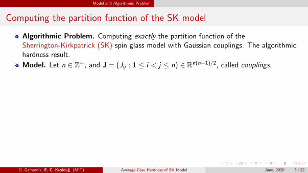
Algorithmic Problem. Computing exactly the partition function of theSherrington-Kirkpatrick (SK) spin glass model with Gaussian couplings. The algorithmichardness result.
Model. Let n ∈ Z+, and J = (Jij : 1 ≤ i < j ≤ n) ∈ Rn(n−1)/2, called couplings.
Consider n sites [n] , {1, 2, . . . , n}, and assign a spin σi ∈ {±1} for each i ∈ [n].
Energy of σ = (σi : i ∈ [n]) ∈ {±1}n at inverse temperature β > 0 given by Hamiltonian
H(σ) =β√n
∑1≤i<j≤n
Jijσiσj .
An algorithm A to exactly compute the partition function
Z (J, β) =∑
σ∈{±1}nexp (−H(σ)) .
D. Gamarnik, E. C. Kızıldag (MIT) Average-Case Hardness of SK Model June, 2020 3 / 22

Model and Algorithmic Problem
Computing the partition function of the SK model
Algorithmic Problem. Computing exactly the partition function of theSherrington-Kirkpatrick (SK) spin glass model with Gaussian couplings. The algorithmichardness result.
Model. Let n ∈ Z+, and J = (Jij : 1 ≤ i < j ≤ n) ∈ Rn(n−1)/2, called couplings.
Consider n sites [n] , {1, 2, . . . , n}, and assign a spin σi ∈ {±1} for each i ∈ [n].
Energy of σ = (σi : i ∈ [n]) ∈ {±1}n at inverse temperature β > 0 given by Hamiltonian
H(σ) =β√n
∑1≤i<j≤n
Jijσiσj .
An algorithm A to exactly compute the partition function
Z (J, β) =∑
σ∈{±1}nexp (−H(σ)) .
D. Gamarnik, E. C. Kızıldag (MIT) Average-Case Hardness of SK Model June, 2020 3 / 22

Model and Algorithmic Problem
Computing the partition function of the SK model
Problem of computing Z (J) for arbitrary J is #P−hard, Valiant [80s].
Computing partition function for arbitrary input is hard for a broader class of statisticalphysics models: Barahona [82], Istrail [00], ...
Requirement. For random J,
P (ZA(J) = Z (J)) ≥ δ,
probability with respect to draw of J.
Thus, our goal is average-case hardness. Classical reduction techniques for worst-casehardness do not transfer.
Of interest in cryptography and TCS. Examples include shortest lattice vector problem(Ajtai [96]), and permanent (Lipton [89], Feige and Lund [92], Cai et al. [99]).
D. Gamarnik, E. C. Kızıldag (MIT) Average-Case Hardness of SK Model June, 2020 4 / 22

Part I: Hardness under Finite Precision Arithmetic.
Overview
1 Model and Algorithmic Problem
2 Part I: Hardness under Finite Precision Arithmetic.Cuts/PolaritiesTruncationMain ResultProof Sketch
3 Part II: Hardness under Real-Valued Model.Setup and ModelMain Result
4 Concluding RemarksExtensionsLimitations and Open Problems
D. Gamarnik, E. C. Kızıldag (MIT) Average-Case Hardness of SK Model June, 2020 5 / 22

Part I: Hardness under Finite Precision Arithmetic.
Part I. Hardness under Finite Precision Arithmetic. Modified Model
Ai , 1 ≤ i ≤ n, independent mean zero normal, called external field. Modified Hamiltonian:
H(σ) =β√n
∑1≤i<j≤n
Jijσiσj +∑
1≤i≤nAiσi .
Corresponding partition function Z1(J,A), where A = (Ai : 1 ≤ i ≤ n).
We study alternative Hamiltonian
H(σ) =β√n
∑1≤i<j≤n
Jijσiσj +∑
1≤i≤nBiσi −
∑1≤i≤n
Ciσi .
Bi , 1 ≤ i ≤ n and Ci , 1 ≤ i ≤ n independent, zero-mean; partition function Z2(J,B,C).
Equivalence: if A1 with input (J,A) computes Z1(J,A) then A1 with input (J,B− C)computes Z2(J,B,C). If A2 with input (Z,B,C) computes Z2(J,B,C) then A2 withinput (J, G+A
2 , G−A2 ) computes Z1(J,A), where G = (Gi : 1 ≤ i ≤ n) i.i.d. copy of A.
D. Gamarnik, E. C. Kızıldag (MIT) Average-Case Hardness of SK Model June, 2020 6 / 22

Part I: Hardness under Finite Precision Arithmetic. Cuts/Polarities
Part I. Hardness under Finite Precision Arithmetic. Cuts/Polarities.
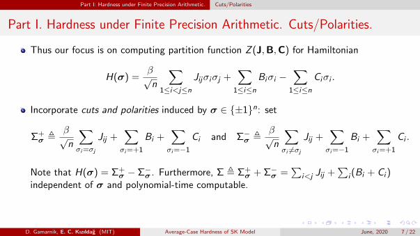
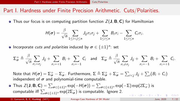
Thus our focus is on computing partition function Z (J,B,C) for Hamiltonian
H(σ) =β√n
∑1≤i<j≤n
Jijσiσj +∑
1≤i≤nBiσi −
∑1≤i≤n
Ciσi .
Incorporate cuts and polarities induced by σ ∈ {±1}n: set
Σ+σ ,
β√n
∑σi=σj
Jij +∑σi=+1
Bi +∑σi=−1
Ci and Σ−σ ,β√n
∑σi 6=σj
Jij +∑σi=−1
Bi +∑σi=+1
Ci .
Note that H(σ) = Σ+σ − Σ−σ . Furthermore, Σ , Σ+
σ + Σ−σ =∑
i<j Jij +∑
i (Bi + Ci )independent of σ and polynomial-time computable.
Thus Z (J,B,C) =∑
σ∈{±1}n exp(−H(σ)) =∑
σ∈{±1}n exp(−Σ) exp(2Σ−σ ) is
computable iff∑
σ∈{±1}n exp(2Σ−σ ) is computable. Ignore 2.
D. Gamarnik, E. C. Kızıldag (MIT) Average-Case Hardness of SK Model June, 2020 7 / 22

Part I: Hardness under Finite Precision Arithmetic. Cuts/Polarities
Part I. Hardness under Finite Precision Arithmetic. Cuts/Polarities.
Thus our focus is on computing partition function Z (J,B,C) for Hamiltonian
H(σ) =β√n
∑1≤i<j≤n
Jijσiσj +∑
1≤i≤nBiσi −
∑1≤i≤n
Ciσi .
Incorporate cuts and polarities induced by σ ∈ {±1}n: set
Σ+σ ,
β√n
∑σi=σj
Jij +∑σi=+1
Bi +∑σi=−1
Ci and Σ−σ ,β√n
∑σi 6=σj
Jij +∑σi=−1
Bi +∑σi=+1
Ci .
Note that H(σ) = Σ+σ − Σ−σ . Furthermore, Σ , Σ+
σ + Σ−σ =∑
i<j Jij +∑
i (Bi + Ci )independent of σ and polynomial-time computable.
Thus Z (J,B,C) =∑
σ∈{±1}n exp(−H(σ)) =∑
σ∈{±1}n exp(−Σ) exp(2Σ−σ ) is
computable iff∑
σ∈{±1}n exp(2Σ−σ ) is computable. Ignore 2.
D. Gamarnik, E. C. Kızıldag (MIT) Average-Case Hardness of SK Model June, 2020 7 / 22

Part I: Hardness under Finite Precision Arithmetic. Truncation
Part I. Hardness under Finite Precision Arithmetic. Truncation.
Let Jij = exp(βJij/√n), Bi = exp(Bi ), and Ci = exp(Ci ).
Truncation: Fix N ∈ Z+, let x [N] , 2−Nb2Nxc. Truncate inputs: J[N]ij , B
[N]i , and C
[N]i .
Goal is to compute
Z (J[N], B[N], C[N]) =∑
σ∈{−1,1}n
∏σi 6=σj
Jij[N]
∏σi=−1
Bi[N]
∏σi=+1
Ci[N]
.
Switching to Integer Inputs: Define Jij , 2N J[N]ij ∈ Z, and Bi , Ci similarly. Focus:
Zn(J, B, C) =∑
σ∈{−1,1}n2Nf (n,σ)
∏σi 6=σj
Jij
∏σi=−1
Bi
∏σi=+1
Ci
,
where f (n,σ) = n(n − 1)/2− n − |{(i , j) : 1 ≤ i < j ≤ n, σi 6= σj}|.Observe that Zn(J, B, C) = 2Nn(n−1)/2Z (J[N], B[N], C[N]) ∈ Z.
D. Gamarnik, E. C. Kızıldag (MIT) Average-Case Hardness of SK Model June, 2020 8 / 22

Part I: Hardness under Finite Precision Arithmetic. Truncation
Part I. Hardness under Finite Precision Arithmetic. Truncation.
Let Jij = exp(βJij/√n), Bi = exp(Bi ), and Ci = exp(Ci ).
Truncation: Fix N ∈ Z+, let x [N] , 2−Nb2Nxc. Truncate inputs: J[N]ij , B
[N]i , and C
[N]i .
Goal is to compute
Z (J[N], B[N], C[N]) =∑
σ∈{−1,1}n
∏σi 6=σj
Jij[N]
∏σi=−1
Bi[N]
∏σi=+1
Ci[N]
.
Switching to Integer Inputs: Define Jij , 2N J[N]ij ∈ Z, and Bi , Ci similarly. Focus:
Zn(J, B, C) =∑
σ∈{−1,1}n2Nf (n,σ)
∏σi 6=σj
Jij
∏σi=−1
Bi
∏σi=+1
Ci
,
where f (n,σ) = n(n − 1)/2− n − |{(i , j) : 1 ≤ i < j ≤ n, σi 6= σj}|.
Observe that Zn(J, B, C) = 2Nn(n−1)/2Z (J[N], B[N], C[N]) ∈ Z.
D. Gamarnik, E. C. Kızıldag (MIT) Average-Case Hardness of SK Model June, 2020 8 / 22

Part I: Hardness under Finite Precision Arithmetic. Truncation
Part I. Hardness under Finite Precision Arithmetic. Truncation.
Let Jij = exp(βJij/√n), Bi = exp(Bi ), and Ci = exp(Ci ).
Truncation: Fix N ∈ Z+, let x [N] , 2−Nb2Nxc. Truncate inputs: J[N]ij , B
[N]i , and C
[N]i .
Goal is to compute
Z (J[N], B[N], C[N]) =∑
σ∈{−1,1}n
∏σi 6=σj
Jij[N]
∏σi=−1
Bi[N]
∏σi=+1
Ci[N]
.
Switching to Integer Inputs: Define Jij , 2N J[N]ij ∈ Z, and Bi , Ci similarly. Focus:
Zn(J, B, C) =∑
σ∈{−1,1}n2Nf (n,σ)
∏σi 6=σj
Jij
∏σi=−1
Bi
∏σi=+1
Ci
,
where f (n,σ) = n(n − 1)/2− n − |{(i , j) : 1 ≤ i < j ≤ n, σi 6= σj}|.Observe that Zn(J, B, C) = 2Nn(n−1)/2Z (J[N], B[N], C[N]) ∈ Z.
D. Gamarnik, E. C. Kızıldag (MIT) Average-Case Hardness of SK Model June, 2020 8 / 22

Part I: Hardness under Finite Precision Arithmetic. Main Result
Part I. Hardness under Finite Precision Arithmetic. Main Result
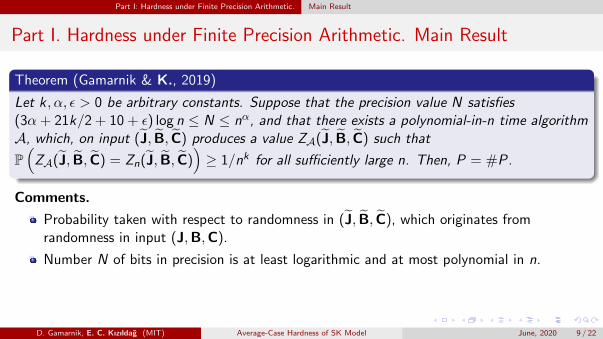
Theorem (Gamarnik & K., 2019)
Let k , α, ε > 0 be arbitrary constants. Suppose that the precision value N satisfies(3α + 21k/2 + 10 + ε) log n ≤ N ≤ nα, and that there exists a polynomial-in-n time algorithmA, which, on input (J, B, C) produces a value ZA(J, B, C) such that
P(ZA(J, B, C) = Zn(J, B, C)
)≥ 1/nk for all sufficiently large n. Then, P = #P.
Comments.
Probability taken with respect to randomness in (J, B, C), which originates fromrandomness in input (J,B,C).
Number N of bits in precision is at least logarithmic and at most polynomial in n.
Upper bound ensures bit stream supplied to algorithm is of polynomial length.
Lower bound required for technical reasons when establishing near-uniformity of (J, B, C).
D. Gamarnik, E. C. Kızıldag (MIT) Average-Case Hardness of SK Model June, 2020 9 / 22

Part I: Hardness under Finite Precision Arithmetic. Main Result
Part I. Hardness under Finite Precision Arithmetic. Main Result
Theorem (Gamarnik & K., 2019)
Let k , α, ε > 0 be arbitrary constants. Suppose that the precision value N satisfies(3α + 21k/2 + 10 + ε) log n ≤ N ≤ nα, and that there exists a polynomial-in-n time algorithmA, which, on input (J, B, C) produces a value ZA(J, B, C) such that
P(ZA(J, B, C) = Zn(J, B, C)
)≥ 1/nk for all sufficiently large n. Then, P = #P.
Comments.
Probability taken with respect to randomness in (J, B, C), which originates fromrandomness in input (J,B,C).
Number N of bits in precision is at least logarithmic and at most polynomial in n.
Upper bound ensures bit stream supplied to algorithm is of polynomial length.
Lower bound required for technical reasons when establishing near-uniformity of (J, B, C).
D. Gamarnik, E. C. Kızıldag (MIT) Average-Case Hardness of SK Model June, 2020 9 / 22

Part I: Hardness under Finite Precision Arithmetic. Proof Sketch
Idea of Proof.
Inspired from average-case hardness proof by Cai et al. [99] for computing permanentover a finite field. Recall that for an A ∈ Rm×m,
permanent(A) =∑σ∈Sn
∏1≤i≤n
ai ,σ(i),
where Sn is the set of all permutations of {1, 2, . . . , n}. #P−hard to compute forarbitrary inputs.
Let Zp be a finite field. Permanent of a M ∈ Zn×np equals to a weighted sum of
permanents of n minors M11, . . . ,Mn1 ∈ Z(n−1)×(n−1)p .
Construct a matrix polynomial whose value at k ∈ {1, 2, . . . , n} is minor Mk1. Thepermanent of this matrix polynomial is a low-degree univariate polynomial. Call it ϕ.
D. Gamarnik, E. C. Kızıldag (MIT) Average-Case Hardness of SK Model June, 2020 10 / 22

Part I: Hardness under Finite Precision Arithmetic. Proof Sketch
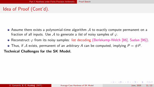
Idea of Proof (Cont’d).
Assume there exists a polynomial-time algorithm A to exactly compute permanent on afraction of all inputs. Use A to generate a list of noisy samples of ϕ.
Reconstruct ϕ from its noisy samples: list decoding (Berlekamp-Welch [86], Sudan [96]).
Thus, if A exists, permanent of an arbitrary A can be computed, implying P = #P.
Technical Challenges for the SK Model.
Not clear if a Laplace-like self-recursion takes place for partition function.
Hardness results above address uniform input over Zp. We have truncated log-normals.
D. Gamarnik, E. C. Kızıldag (MIT) Average-Case Hardness of SK Model June, 2020 11 / 22

Part I: Hardness under Finite Precision Arithmetic. Proof Sketch
Idea of Proof (Cont’d).
Assume there exists a polynomial-time algorithm A to exactly compute permanent on afraction of all inputs. Use A to generate a list of noisy samples of ϕ.
Reconstruct ϕ from its noisy samples: list decoding (Berlekamp-Welch [86], Sudan [96]).
Thus, if A exists, permanent of an arbitrary A can be computed, implying P = #P.
Technical Challenges for the SK Model.
Not clear if a Laplace-like self-recursion takes place for partition function.
Hardness results above address uniform input over Zp. We have truncated log-normals.
D. Gamarnik, E. C. Kızıldag (MIT) Average-Case Hardness of SK Model June, 2020 11 / 22

Part I: Hardness under Finite Precision Arithmetic. Proof Sketch
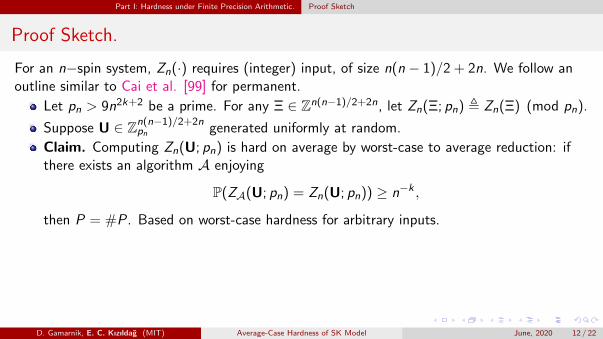
Proof Sketch.
For an n−spin system, Zn(·) requires (integer) input, of size n(n − 1)/2 + 2n. We follow anoutline similar to Cai et al. [99] for permanent.
Let pn > 9n2k+2 be a prime. For any Ξ ∈ Zn(n−1)/2+2n, let Zn(Ξ; pn) , Zn(Ξ) (mod pn).
Suppose U ∈ Zn(n−1)/2+2npn generated uniformly at random.
Claim. Computing Zn(U; pn) is hard on average by worst-case to average reduction: ifthere exists an algorithm A enjoying
P(ZA(U; pn) = Zn(U; pn)) ≥ n−k ,
then P = #P. Based on worst-case hardness for arbitrary inputs.
Downward self-reduction from n−spin system to (n − 1)−spin system: for someparameters B ′n,C
′n ∈ Zpn and B+,B−,C+,C− ∈ Zn−1
pn , it holds:
Zn(J,B,C; pn) = C ′nZn−1(J′,B+,C+; pn) + B ′nZn−1(J′,B−,C−; pn).
Analogous to Laplace expansion for permanent.
D. Gamarnik, E. C. Kızıldag (MIT) Average-Case Hardness of SK Model June, 2020 12 / 22

Part I: Hardness under Finite Precision Arithmetic. Proof Sketch
Proof Sketch.
For an n−spin system, Zn(·) requires (integer) input, of size n(n − 1)/2 + 2n. We follow anoutline similar to Cai et al. [99] for permanent.
Let pn > 9n2k+2 be a prime. For any Ξ ∈ Zn(n−1)/2+2n, let Zn(Ξ; pn) , Zn(Ξ) (mod pn).
Suppose U ∈ Zn(n−1)/2+2npn generated uniformly at random.
Claim. Computing Zn(U; pn) is hard on average by worst-case to average reduction: ifthere exists an algorithm A enjoying
P(ZA(U; pn) = Zn(U; pn)) ≥ n−k ,
then P = #P. Based on worst-case hardness for arbitrary inputs.
Downward self-reduction from n−spin system to (n − 1)−spin system: for someparameters B ′n,C
′n ∈ Zpn and B+,B−,C+,C− ∈ Zn−1
pn , it holds:
Zn(J,B,C; pn) = C ′nZn−1(J′,B+,C+; pn) + B ′nZn−1(J′,B−,C−; pn).
Analogous to Laplace expansion for permanent.
D. Gamarnik, E. C. Kızıldag (MIT) Average-Case Hardness of SK Model June, 2020 12 / 22

Part I: Hardness under Finite Precision Arithmetic. Proof Sketch
Proof Sketch.
For an n−spin system, Zn(·) requires (integer) input, of size n(n − 1)/2 + 2n. We follow anoutline similar to Cai et al. [99] for permanent.
Let pn > 9n2k+2 be a prime. For any Ξ ∈ Zn(n−1)/2+2n, let Zn(Ξ; pn) , Zn(Ξ) (mod pn).
Suppose U ∈ Zn(n−1)/2+2npn generated uniformly at random.
Claim. Computing Zn(U; pn) is hard on average by worst-case to average reduction: ifthere exists an algorithm A enjoying
P(ZA(U; pn) = Zn(U; pn)) ≥ n−k ,
then P = #P. Based on worst-case hardness for arbitrary inputs.
Downward self-reduction from n−spin system to (n − 1)−spin system: for someparameters B ′n,C
′n ∈ Zpn and B+,B−,C+,C− ∈ Zn−1
pn , it holds:
Zn(J,B,C; pn) = C ′nZn−1(J′,B+,C+; pn) + B ′nZn−1(J′,B−,C−; pn).
Analogous to Laplace expansion for permanent.D. Gamarnik, E. C. Kızıldag (MIT) Average-Case Hardness of SK Model June, 2020 12 / 22

Part I: Hardness under Finite Precision Arithmetic. Proof Sketch
Proof Sketch.
Recall. The object of interest satisfies
Zn(J,B,C; pn) = C ′nZn−1(J′,B+,C+; pn)+B′nZn−1(J′,B−,C−; pn).
Construct a vector polynomial D(x) such that D(1) = (J′,B+,C+) andD(2) = (J′,B−,C−). D(x) thought of as a vector carrying parameters required for an(n − 1)−spin system.
Let φ(x) = Zn(D(x); pn), associated partition function. φ(·) is univariate polynomial, ofdegree at most n2.
Note thatZn(J,B,C; pn) = C ′nφ(1) + B ′nφ(2).
Thus Zn can be computed provided φ(·) can be reconstructed.
D. Gamarnik, E. C. Kızıldag (MIT) Average-Case Hardness of SK Model June, 2020 13 / 22

Part I: Hardness under Finite Precision Arithmetic. Proof Sketch
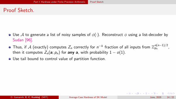
Proof Sketch.
Use A to generate a list of noisy samples of φ(·). Reconstruct φ using a list-decoder bySudan [96].
Thus, if A (exactly) computes Zn correctly for n−k fraction of all inputs from Zn(n−1)/2pn ,
then it computes Zn(a; pn) for any a, with probability 1− o(1).
Use tail bound to control value of partition function.
Use prime density to take sufficiently many primes, product larger than partition function.Apply Chinese remaindering.
D. Gamarnik, E. C. Kızıldag (MIT) Average-Case Hardness of SK Model June, 2020 14 / 22

Part I: Hardness under Finite Precision Arithmetic. Proof Sketch
Proof Sketch.
Use A to generate a list of noisy samples of φ(·). Reconstruct φ using a list-decoder bySudan [96].
Thus, if A (exactly) computes Zn correctly for n−k fraction of all inputs from Zn(n−1)/2pn ,
then it computes Zn(a; pn) for any a, with probability 1− o(1).
Use tail bound to control value of partition function.
Use prime density to take sufficiently many primes, product larger than partition function.Apply Chinese remaindering.
D. Gamarnik, E. C. Kızıldag (MIT) Average-Case Hardness of SK Model June, 2020 14 / 22

Part I: Hardness under Finite Precision Arithmetic. Proof Sketch
Proof Sketch.
Rest is a probabilistic coupling argument.
Recall Jij = 2N J[N]ij , where J
[N]ij = 2−Nb2N Jijc, and Jij = exp(βJijn
−1/2). Recall also
Bi , Ci .
Show Jij , Bi , Ci modulo pn are close to uniform distribution.
Use coupling idea to conclude.
D. Gamarnik, E. C. Kızıldag (MIT) Average-Case Hardness of SK Model June, 2020 15 / 22

Part II: Hardness under Real-Valued Model.
Overview
1 Model and Algorithmic Problem
2 Part I: Hardness under Finite Precision Arithmetic.Cuts/PolaritiesTruncationMain ResultProof Sketch
3 Part II: Hardness under Real-Valued Model.Setup and ModelMain Result
4 Concluding RemarksExtensionsLimitations and Open Problems
D. Gamarnik, E. C. Kızıldag (MIT) Average-Case Hardness of SK Model June, 2020 16 / 22

Part II: Hardness under Real-Valued Model. Setup and Model
Part II. Hardness under Real-Valued Model. Setup and Model
Hardness when computational engine (e.g. Blum-Shub-Smale machine) operates overreal-valued inputs. Each arithmetic operation has unit cost.
We consider Hamiltonian without external field: H(σ) =∑
i<j Jijσiσj .
Scaling√n and inverse temperature β suppressed for simplicity.
After reducing to cuts analogously, boils down computing
Z (J) =∑
σ∈{±1}nexp
∑σi 6=σj
2Jij
.
Techniques of previous setting tailored to finite precision model: finite field structure Zp islost upon passing real-valued model. By pass through an argument by Aaronson andArkhipov [2011].
D. Gamarnik, E. C. Kızıldag (MIT) Average-Case Hardness of SK Model June, 2020 17 / 22

Part II: Hardness under Real-Valued Model. Main Result
Part II. Hardness under Real-Valued Model: Main result
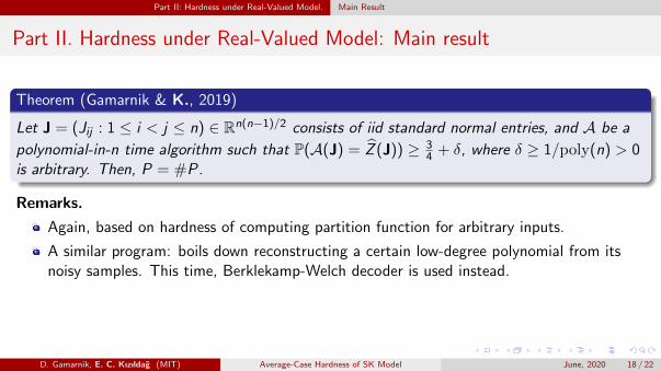
Theorem (Gamarnik & K., 2019)
Let J = (Jij : 1 ≤ i < j ≤ n) ∈ Rn(n−1)/2 consists of iid standard normal entries, and A be a
polynomial-in-n time algorithm such that P(A(J) = Z (J)) ≥ 34 + δ, where δ ≥ 1/poly(n) > 0
is arbitrary. Then, P = #P.
Remarks.
Again, based on hardness of computing partition function for arbitrary inputs.
A similar program: boils down reconstructing a certain low-degree polynomial from itsnoisy samples. This time, Berklekamp-Welch decoder is used instead.
Uses a control for total variation distance for log-normal random variables, in presence ofa convex perturbation.
D. Gamarnik, E. C. Kızıldag (MIT) Average-Case Hardness of SK Model June, 2020 18 / 22

Part II: Hardness under Real-Valued Model. Main Result
Part II. Hardness under Real-Valued Model: Main result
Theorem (Gamarnik & K., 2019)
Let J = (Jij : 1 ≤ i < j ≤ n) ∈ Rn(n−1)/2 consists of iid standard normal entries, and A be a
polynomial-in-n time algorithm such that P(A(J) = Z (J)) ≥ 34 + δ, where δ ≥ 1/poly(n) > 0
is arbitrary. Then, P = #P.
Remarks.
Again, based on hardness of computing partition function for arbitrary inputs.
A similar program: boils down reconstructing a certain low-degree polynomial from itsnoisy samples. This time, Berklekamp-Welch decoder is used instead.
Uses a control for total variation distance for log-normal random variables, in presence ofa convex perturbation.
D. Gamarnik, E. C. Kızıldag (MIT) Average-Case Hardness of SK Model June, 2020 18 / 22

Concluding Remarks
Overview
1 Model and Algorithmic Problem
2 Part I: Hardness under Finite Precision Arithmetic.Cuts/PolaritiesTruncationMain ResultProof Sketch
3 Part II: Hardness under Real-Valued Model.Setup and ModelMain Result
4 Concluding RemarksExtensionsLimitations and Open Problems
D. Gamarnik, E. C. Kızıldag (MIT) Average-Case Hardness of SK Model June, 2020 19 / 22

Concluding Remarks Extensions
Concluding Remarks : Extensions
Average-case hardness of algorithmic problem of exactly computing partition function ofSK spin glass model. Under both finite precision arithmetic and real-valued computationalmodels.
To the best of our knowledge, first such average-case hardness result for a statisticalphysics model.
Extensions.
2−spin assumption is non-essential: extends to the p−spin models.
Gaussianity of the couplings is non-essential. Well behaved distributions with sufficientlysmooth density should be enough.
The scaling n−12 is non-essential: any constant power of n is ok.
D. Gamarnik, E. C. Kızıldag (MIT) Average-Case Hardness of SK Model June, 2020 20 / 22

Concluding Remarks Limitations and Open Problems
Concluding Remarks : Limitations and Open Problems
Our approach does not treat the same problem when couplings are i.i.d. Rademacher.Not surprising though in light of the fact that average-case hardness of computingpermanent of a binary matrix is open as well.
The trick of (mod pn) computation is too ”fragile” to survive the approximatecomputation: average-case hardness of computing Z (J, β) to within a multiplicativefactor of 1± ε remains open.
A related problem: Ground-state computation. σ∗ ∈ {±1}n is called a ground-state ifH(σ∗) = maxσ∈{±1}n H(σ).
Arora et al. [05]: problem of computing ground state is NP-hard (in worst-case sense).
Montanari [19]: a message-passing algorithm, which for any ε > 0, finds (in time O(n2))a state σ∗ ∈ {±1}n such that H(σ∗) ≥ (1− ε)H(σ∗) whp.
Average-case hardness of problem of exactly computing σ∗ remains open: algebraicstructure is lost upon passing to maximization.
D. Gamarnik, E. C. Kızıldag (MIT) Average-Case Hardness of SK Model June, 2020 21 / 22

Concluding Remarks Limitations and Open Problems
Thank you!
D. Gamarnik, E. C. Kızıldag (MIT) Average-Case Hardness of SK Model June, 2020 22 / 22