Computing the Market Price of Volatility Risk in the Energy Commodity Markets
20
Computing the Market Price of Volatility Risk in the Energy Commodity Markets James S. Doran Department of Finance Florida State University Ehud I. Ronn Department of Finance University of Texas at Austin January 2007
Transcript of Computing the Market Price of Volatility Risk in the Energy Commodity Markets

Computing the Market Price of Volatility Risk in the Energy
Commodity MarketsJames S. Doran
Department of FinanceFlorida State University
Ehud I. RonnDepartment of Finance
University of Texas at Austin
January 2007
Dr. James S. Doran, Department of Finance, Florida State Universitygarnet.acns.fsu.edu/~jsdoran
2
Outline and Overview
The relationship between implied and realized volatility in energy marketsInstantaneous parameter sensitivities demonstrated via quasi‐Monte‐Carlo simulationMarket price of volatility risk estimation

Dr. James S. Doran, Department of Finance, Florida State Universitygarnet.acns.fsu.edu/~jsdoran
3
Motivation and ContributionBridge two strands of literature and extend one:
Quantify the bias between implied volatility and realized volatility Relate the bias in Black‐Scholes to the underlying parametersExtend our understanding of risk premium in energy markets
Relate the Market Price of Volatility Risk (λσ) to F<E(ST) for equitiesWhy option traders like to be shortF>E(ST) for commodities
Demonstrate the differences between commodity and equity markets
Positive skew in commodities marketsRelationship between price and volatility

Dr. James S. Doran, Department of Finance, Florida State Universitygarnet.acns.fsu.edu/~jsdoran
4
Literature ReviewData Generating Process
Black‐Scholes (1972)Hull and White (1987), Heston (1993)Bates (1994, 1996), Duffie, Pan and Singleton (2000), Pan (2002)
Market Price of Volatility RiskCoval and Sumway (2001)Buraschi and Jackwerth (2001)Carr and Wu (2004)Doran (2007)
Energy RiskSchwartz (1997), Schwartz and Smith (2000)Hilliard and Reis (1998)Pindyck (1999)Casassus and Collin Dufresne (2005)Doran and Ronn (2006)

Dr. James S. Doran, Department of Finance, Florida State Universitygarnet.acns.fsu.edu/~jsdoran
5
Preview of Results
The inclusion of a market price of volatility risk appears necessary to capture the degree of bias in BSIV/BIVThe market price of volatility risk is negative and significant for natural gas, crude oil, and heating oil. There is a seasonality in the volatility risk premium for natural gas

Dr. James S. Doran, Department of Finance, Florida State Universitygarnet.acns.fsu.edu/~jsdoran
6
Pricing Dynamics
This is not a test of spot and futures price relationship
i.e, Schwartz (1997)
This is an option on futures
Start with traditional equity literature

Dr. James S. Doran, Department of Finance, Florida State Universitygarnet.acns.fsu.edu/~jsdoran
7
Data Generating Process
Must have two distinct price treesRisk Neutral Process
Real World Process
Jump arrives at γdt for risk-neutral processJump arrives at γ(1−λ)dt for real world processJump size is drawn from N~(μj∗,σ2) for risk-neutral processJump size is drawn from N~(μj,σ2) for real world process
SV‐ModelSVJ0‐Model

Dr. James S. Doran, Department of Finance, Florida State Universitygarnet.acns.fsu.edu/~jsdoran
8
Monte Carlo & Quasi Monte Carlo
Simulate processes over n pathN=30,000Sobol Sequence
( )∑=
− −=N
iTi
rT KSeN
Call1
* )0,max(1
),0(~,,,252/1
** tNdzdzdzdzt
sS Δ
Δ
σσ
=
TSSN
N
iTi ])/[ln(1
101 ∑
=
−= μσ
)(11
2,2 ∑
=
−=t
ktkt rr
τ
τσ
Implied Volatility
Realized Volatility

Dr. James S. Doran, Department of Finance, Florida State Universitygarnet.acns.fsu.edu/~jsdoran
9
Simulated Volatility DifferenceThis table highlights the simulated percentage difference in Black implied volatility (BIV) versus realized volatility using the SVJ (stochastic volatility with jumps) model and the SVJ0 (stochastic volatility with jump but no market price of volatility risk) model. In each case the simulation is conducted over 30 days (22‐trading days) using the given futures
contract and a corresponding ATM option.

Dr. James S. Doran, Department of Finance, Florida State Universitygarnet.acns.fsu.edu/~jsdoran
10
Volatility SkewFigure 1 demonstrates the simulated volatility difference between implied and realized
volatility across the cross‐section of option prices using the SVJ model.

Dr. James S. Doran, Department of Finance, Florida State Universitygarnet.acns.fsu.edu/~jsdoran
11
Data
Daily observations for natural gas, crude oil, and heating oil futures and optionsContracts expiring between January 1995 through December 2005Use only close to ATM optionsData comes from Bloomberg and NYMEX

Dr. James S. Doran, Department of Finance, Florida State Universitygarnet.acns.fsu.edu/~jsdoran
12
Descriptive Statistics for Monthly Energy ContractsThe number of observations for natural gas, crude oil, and heating oil are 26,843, 27,065,
and 22,827 respectively.

Dr. James S. Doran, Department of Finance, Florida State Universitygarnet.acns.fsu.edu/~jsdoran
13
Implied Volatility in Energy MarketsFigure 2 demonstrates the implied volatility of the near‐term contract for the three energy commodities and VIX, the weighted average of implied volatility on near‐term S&P 500 option contracts. The implied volatility for each energy commodity comes
from the contract that is closest to maturity up until 10‐days to expiration. The second near‐term month then is used instead. HO is the implied volatility from heating oil contracts, CO is from crude oil contracts, and NG is from natural gas contracts. The
period is from January 1994 through April 2004.

Dr. James S. Doran, Department of Finance, Florida State Universitygarnet.acns.fsu.edu/~jsdoran
14
Solving for the Instantaneous Parameters
Estimate the risk‐neutral parameters
Reciprocal specification to capture TSOVSimilar to Dennis, Mayhew, and Stivers (2006)Alternatively, to capture monthly effects using December as the base month

Dr. James S. Doran, Department of Finance, Florida State Universitygarnet.acns.fsu.edu/~jsdoran
15Risk Neutral ParametersThis table reports the parameter estimates of the mean‐reverting regression for three energy commodities: natural gas, crude oil, and heating oil. The period uses daily frequency from monthly contracts between 1994 through 2005, over the period January 1994 through April 2004. Each commodity is estimated using equations (15‐16), where equation (16) controls for potential year effects. Monthly dummies, MON, are included for each of the j contract months, using December as thebase month. The term‐structure control uses a reciprocal specification, where DM is the number of days until maturity
divided by 360

Dr. James S. Doran, Department of Finance, Florida State Universitygarnet.acns.fsu.edu/~jsdoran
16
Solving for the Volatility Risk Premium
Calibrate the data generating process by minimizing the difference between the estimated and actual implied and realized volatility
Done in a similar spirit to Bakshi, Cao, and Chen (1997) and Bates (2000)Estimate volatilities using quasi‐Monte Carlo and the given data‐generated process
Dr. James S. Doran, Department of Finance, Florida State Universitygarnet.acns.fsu.edu/~jsdoran
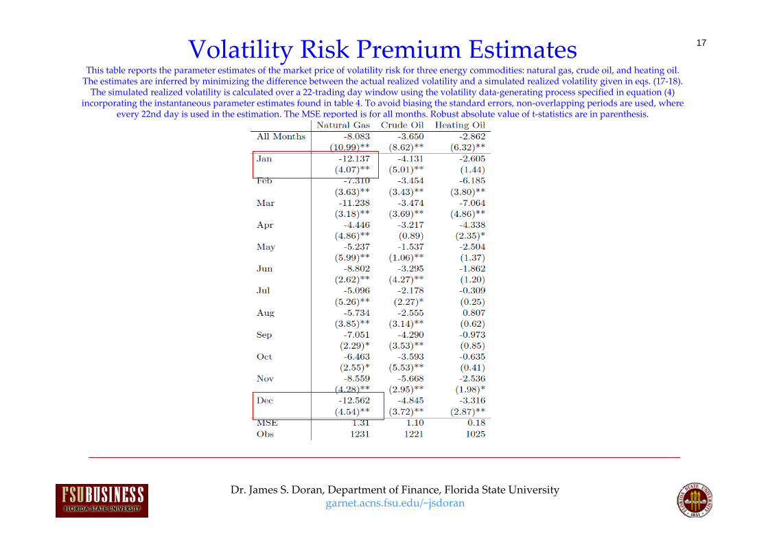
17Volatility Risk Premium EstimatesThis table reports the parameter estimates of the market price of volatility risk for three energy commodities: natural gas, crude oil, and heating oil. The estimates are inferred by minimizing the difference between the actual realized volatility and a simulated realized volatility given in eqs. (17‐18). The simulated realized volatility is calculated over a 22‐trading day window using the volatility data‐generating process specified in equation (4)
incorporating the instantaneous parameter estimates found in table 4. To avoid biasing the standard errors, non‐overlapping periods are used, where every 22nd day is used in the estimation. The MSE reported is for all months. Robust absolute value of t‐statistics are in parenthesis.

Dr. James S. Doran, Department of Finance, Florida State Universitygarnet.acns.fsu.edu/~jsdoran
18
Robustness
Prior results place strong restrictions on the data generating processAdopt the Broadie, Chernov, and Johannes (2006) methodology, but ignore the jump premiumApply GMM methodology using both volatility and return

Dr. James S. Doran, Department of Finance, Florida State Universitygarnet.acns.fsu.edu/~jsdoran
19
Risk Premium across Months

Dr. James S. Doran, Department of Finance, Florida State Universitygarnet.acns.fsu.edu/~jsdoran
20
Conclusions
A negative market price of volatility risk can explain the difference between implied and realized volatilityResults appear consistent with empirical observations
Additional supporting evidence for negative volatility risk premium
How important is the specificationPotential justification for option tradingOption price includes volatility premium