Computer Vision on Mars Vision on Mars LARRY MATTHIES, MARK MAIMONE, ... 1992). This algorithm used...

International Journal of Computer Vision

c© 2007 Springer Science + Business Media, LLC. Manufactured in the United States.

DOI: 10.1007/s11263-007-0046-z

Computer Vision on Mars

LARRY MATTHIES, MARK MAIMONE, ANDREW JOHNSON, YANG CHENG, REG WILLSON,CARLOS VILLALPANDO, STEVE GOLDBERG, AND ANDRES HUERTAS

Jet Propulsion Laboratory, California Institute of Technology, 4800 Oak Grove Drive, Pasadena, CA 91109, [email protected]

[email protected]

[email protected]

[email protected]

[email protected]

[email protected]

[email protected]

[email protected]

ANDREW STEINCarnegie Mellon University, 5000 Forbes Avenue, Pittsburgh, PA 15213, USA

[email protected]

ANELIA ANGELOVACalifornia Institute of Technology, 1200 East California Boulevard, Pasadena, CA 91125, USA

[email protected]

Received May 16, 2006; Accepted February 20, 2007

Abstract. Increasing the level of spacecraft autonomy is essential for broadening the reach of solar system exploration.Computer vision has and will continue to play an important role in increasing autonomy of both spacecraft and Earth-based robotic vehicles. This article addresses progress on computer vision for planetary rovers and landers and has fourmain parts. First, we review major milestones in the development of computer vision for robotic vehicles over the lastfour decades. Since research on applications for Earth and space has often been closely intertwined, the review includeselements of both. Second, we summarize the design and performance of computer vision algorithms used on Mars inthe NASA/JPL Mars Exploration Rover (MER) mission, which was a major step forward in the use of computer visionin space. These algorithms did stereo vision and visual odometry for rover navigation and feature tracking for horizontalvelocity estimation for the landers. Third, we summarize ongoing research to improve vision systems for planetaryrovers, which includes various aspects of noise reduction, FPGA implementation, and vision-based slip perception.Finally, we briefly survey other opportunities for computer vision to impact rovers, landers, and orbiters in future solarsystem exploration missions.

Keywords: stereo vision, obstacle detection, visual odometry, visual velocity estimation, slip prediction, planetaryexploration

1. Introduction

Both on Earth and in space, a key motivation for de-veloping computer vision-based, autonomous navigationsystems is that communication latency and bandwidth

limitations severely constrain the ability of humans tocontrol robot functions remotely. In space, onboard com-puter vision enables rovers to explore planetary surfacesmore quickly and safely, landers to land more safelyand precisely, and orbiters to better maintain safe orbits

Matthies et al.

in the weak and uneven gravity fields of small aster-oids, comets, and moons. The performance limitationsof space-qualified computers strongly constrain the com-plexity of onboard vision algorithms. Nevertheless, theMER mission, which landed two rovers on Mars in 2004,very successfully used stereo vision, visual odometry, andfeature tracking for rover navigation and for estimatingthe horizontal velocity of the landers before touchdown.This was the first use of such algorithms in a planetaryexploration mission. More advanced capabilities, usingmore advanced spaceflight computers, are now of interestfor future missions.

This paper starts with a historical perspective on thefour decades of research that led up to the autonomousnavigation capabilities in MER (Section 2), then de-scribes the design and performance of the MER vi-sion systems (Section 3), ongoing research to improvethem (Section 4), and other opportunities for computervision to impact rover, lander, and orbiter missions(Section 5). The history of planetary rover research istightly interwined with research on robots for Earth-bound applications, since this work has proceeded in par-allel, served related requirements, often been done by thesame people, and experienced much cross-fertilization.Therefore, the historical perspective touches on high-lights of both.

In discussing the MER mission itself, we summarizepertinent characteristics of the mission, the rover, andthe lander, then we briefly describe the algorithms,present main results of their operation in the mission,and note their key limitations. Rover navigation usedstereo cameras for 3-D perception and visual odometry.Computing was performed by a 20 MHz “RAD6000”flight computer, which is a space-qualified version of anearly PowerPC architecture. The lander used one descentcamera and the same flight computer to track featuresover three frames in the last 2 km of descent to thesurface, in order to estimate terrain-relative horizontalvelocity so that retro-rockets could reduce that velocity,if necessary, to avoid tearing the airbags on impact.Since these algorithms and results are discussed in detailelsewhere, we keep the discussion to an overview andprovide references for more detail.

Ongoing research on vision for rover navigation ad-dresses both engineering and research-oriented ends ofthe spectrum. At the engineering end of the spectrum,work on stereo includes FPGA implementation, to in-crease speed in a space-qualifiable architecture, and im-proved algorithms for rectification, prefiltering, and cor-relation to reduce noise, improve performance at occlud-ing boundaries (edges of rocks), and reduce pixel-lockingartifacts. At the research-oriented end of the spectrum,one of the major navigation safety and performance issuesin MER was slippage on sloping terrain. Visual odome-try addressed this to some degree for MER, but we are

now applying learning algorithms to attempt to predictthe amount of slip to expect from the appearance andslope angle of hills immediately in front of the rover.

The most significant possibilities to impact future mis-sions are to improve position estimation for precisionlanding, to detect landing hazards, and to improve station-keeping and orbit estimation around low-gravity bodies,including small asteroids, comets, and moons of the outerplanets. Sensors and algorithms are in development forall of these functions at JPL and elsewhere.

2. Historical Perspective

Planetary rover research began in the early 1960s withanalysis and prototype development of a robotic lu-nar rover for NASA’s Surveyor program (Bekker, 1964)(Table 1, Fig. 1). The U.S. never sent an unmanned roverto the moon, but the Soviet Union sent two teleoper-ated “Lunokhod” rovers in the early 1970s (A ScientificRationale for Mobility in Planetary Environments, 1999).Research on more automated navigation of rovers forMars continued through the 1970s at JPL, Stanford Uni-versity, and elsewhere, using onboard stereo camerasand scanning laser rangefinders and off-board computers(O’Handley, 1973; Levine et al., 1973; Thompson, 1977;Lewis and Johnston, 1977; Gennery, 1980; Moravec,1980).

In the early 1980s, there was a hiatus in planetary roverfunding from NASA, but mobile robot research contin-ued under funding from other agencies at various researchcenters. At Carnegie Mellon University (CMU), Moravecdeveloped a series of mobile robots using stereo visionfor perception (Moravec, 1983). One product of this lineof work was a stereo vision-based visual odometry algo-rithm that produced the first quantitatively accurate stereovision-based egomotion estimation results (Matthies andShafer, 1987) and led to the visual odometry algorithmnow in use on Mars.

Computer vision for mobile robots got a major boostin this period with the start of the DARPA Strategic Com-puting (SC) and Autonomous Land Vehicle (ALV) pro-grams. One goal of SC was to demonstrate vision andadvanced computing results from SC on robotic vehiclesdeveloped under ALV. At CMU, Takeo Kanade was aPrincipal Investigator in both of these programs. UnderSC, Kanade initiated a long-running effort to develop faststereo vision implementations on special-purpose com-puting hardware, commencing with an implementationon the “Warp” systolic array computer at CMU (Guerraand Kanade, 1985).

Robot vehicles built under the ALV program, includingthe CMU “Navlab”, a converted Chevy van, were possi-bly the first to have enough onboard computing power tohost substantial terrain perception, terrain mapping, andpath planning algorithms onboard. ALV-related research


Table 1. Chronology of sample ground robot systems and programs

Period Robot system/program

Mid 1960s Robotic lunar rover prototypes for NASA Surveyor program

Early 1970s Russian Lunokhod lunar rovers

1970s Stanford Cart

Mid-late 1980s DARPA Autonomous Land Vehicle (ALV) Program; first CMU Navlab

1995 “No-Hands Across America” road-following demo by CMU Navlab 5

Late 1980s-early 1990s CMU Ambler

Late 1980s-early 1990s JPL Robby

1992–1996 DARPA “Demo II” Unmanned Ground Vehicle (UGV) Program

1997 Mars Pathfinder mission with Sojourner rover

1997–2002 DARPA Tactical Mobile Robotics (TMR) Program

1998–2001 Demo III Experimental Unmanned Vehicle (XUV)

2001-present Robotics Collaborative Technology Alliance

2000–2003 DARPA Perception for Off-road Robotics (PerceptOR) Program

2003-present Mars Exploration Rover mission with Spirit and Opportunity

2004–2007 DARPA Learning Applied to Ground Robotics (LAGR) Program

2004–2005 DARPA Grand Challenge (1 and 2) desert robot race

Figure 1. Sample ground robots. Top: Surveyor lunar rover prototype, Lunokhod 1, CMU Navlab 1. Middle: JPL Robby Mars rover testbed, CMU

Ambler Mars rover testbed, CMU Dante. Bottom: Demo II UGV, Demo III XUV, DARPA TMR testbed.

Matthies et al.

under Kanade and colleagues focused on road-followingwith monocular, color imagery and on terrain mappingand obstacle avoidance with a two-axis scanning laserrangefinder (ladar) built by the Environmental ResearchInstitute of Michigan (ERIM). By the end of the decade,the Navlab was able to follow a variety of structuredand unstructured roads and avoid obstacles in modestlyrough off-road terrain at speeds from a few kilometers perhour (kph) off-road to 28 kph on structured roads (Thorpeet al., 1991a,b). This was the beginning of an extensive,ongoing body of work at CMU on both road-followingand terrain mapping for off-road navigation by a series ofstudents and more junior faculty. Highlights of this bodyof work include such achievements as the “No-HandsAcross America” trip by Navlab 5 from Pittsburgh toSan Diego, which covered 2849 miles with 98.2% of itautonomous (Pomerleau and Jochem, 1996). Work withthe ERIM ladar produced a number of techniques forregistering and fusing sequences of range images intoaggregate terrain maps and for doing obstacle detectionand avoidance with such maps (Hebert et al., 1988). Ter-rain mapping and analysis for off-road obstacle avoidanceremains an open, active area of research 20 years later.

In the mid-to-late 1980s, NASA resumed funding re-search on autonomous navigation for Mars rovers, withJPL and CMU as the primary participants. The initialco-Principal Investigators at CMU were Kanade, TomMitchell, and Red Whittaker. CMU carried over its ladar-based work from the ALV program into the planetaryrover domain (Hebert et al., 1989), while JPL exploredthe use of stereo vision as an all-solid-state approach thatmight be more easily space qualifiable. CMU built a six-legged robot over 4 m tall called Ambler, to be able to stepover 1 m tall obstacles, and developed perception, plan-ning, and control algorithms for statically stable leggedlocomotion (Krotkov and Simmons, 1996). This was fol-lowed at CMU by a series of NASA-funded projects ledby Whittaker to develop mobile robots (Dante I and DanteII) for major field campaigns on Earth, including descend-ing into volcanoes in Antarctica and Alaska (Wettergreenet al., 1993; Bares and Wettergreen, 1999). Dante II in-cluded a novel ladar mounted on a central mast with a360 degree, spiral scan pattern to do 360 degree mappingaround the robot. JPL’s effort achieved a breakthroughin real-time, area-based stereo vision algorithms that en-abled the first stereo vision-guided autonomous, off-roadtraverse (Matthies, 1992). This algorithm used SSD cor-relation, implemented with efficient sliding sums andapplied at low resolution to bandpass filtered imagery.Implemented on a Motorola 68020 CPU and Datacubeconvolution hardware, the system produced 64 × 60 pixelrange imagery at 0.5 Hz. This success shifted the focus ofstereo vision research from edge-based methods to area-based methods and inspired other robotic vehicle projectsto experiment more with stereo.

The 1990s was a period of tremendous progress, en-abled by more powerful computing and better 3-D sen-sors. The DARPA Unmanned Ground Vehicle (UGV)program built robotic HMMWVs relying on stereo vi-sion for 3-D perception (Mettala, 1992). Autonomousoff-road runs of up to 2 km at 8 kph were achieved witha stereo system that generated range data in a 256 × 45pixel region of interest at about 1.3 Hz (Matthies et al.,1996). This program also experimented for the first timewith stereo vision at night using thermal infrared cam-eras (Matthies et al., 1996; Hebert et al., 1996). Con-currently, Okutomi and Kanade developed an influential,SAD-based, multi-baseline stereo algorithm (Okutomiand Kanade, 1993), which Kanade and co-workers ex-tended in a custom hardware implementation as the CMUVideo-Rate Stereo Machine (Kanade et al., 1996). Thisproduced 256 × 240 disparity maps at 30 Hz. A softwareversion of this algorithm was evaluated for obstacle de-tection on highways at speeds up to 25 mph (Williamson,1998). When Konolige showed that SAD-based stereo al-gorithms could run at up to 30 Hz for 320 × 240 imageryusing only current DSPs or microprocessors (Konolige,1997), emphasis shifted away from special-purpose hard-ware implementations.

The 1990s also saw relatively sophisticated sensorsand autonomous navigation functions migrate into smallrobots. In the DARPA Tactical Mobile Robotics (TMR)program, tracked robots less than one meter long wereequipped with stereo vision and/or SICK single-axisscanning laser rangefinders and programmed to do obsta-cle mapping and avoidance, vision-guided stair climbing,and indoor mapping of hallway networks (Krotkov andBlitch, 1999; Matthies et al., 2002; Thrun, 2001). In thisperiod, NASA refocused on small rovers for affordabil-ity reasons and landed the Sojourner rover on Mars inthe 1997 Mars Pathfinder mission (Wilcox and Nguyen,1998). Since Sojourner’s computer was only an Intel 8085clocked at 2 MHz, its 3-D perception system was a sim-ple light-stripe sensor that measured about 25 elevationpoints in front of the rover (Matthies et al., 1995). Thelander had a multispectral stereo camera pair on a pan/tiltmast about 1.5 m high. Processing this stereo imagery onEarth with JPL’s real-time stereo algorithm produced ex-cellent maps of the terrain around the lander for roveroperators to use in planning the mission. This was val-idation of the performance of the stereo algorithm withreal Mars imagery.

Major outdoor autonomous robot research programsin the 2000s to date include the Demo III Experimen-tal Unmanned Vehicle (Demo III XUV) and RoboticsCollaborative Technology Alliance (RCTA) programs,both funded by the Army Research Lab (ARL), theDARPA Perception for Off-Road Robotics (PerceptOR)and Learning Applied to Ground Robotics (LAGR) pro-grams, and NASA’s Mars Exploration Rover (MER)


mission and supporting technology development. DemoIII, RCTA, and PerceptOR addressed off-road navigationin more complex terrain and, to some degree, day/night,all-weather, and all-season operation. A Demo III follow-on activity, PerceptOR, and LAGR also involved system-atic, quantitative field testing. For results of DemoIII,RCTA, and PerceptOR, see (Shoemaker and Bornstein,2000; Technology Development for Army UnmannedGround Vehicles, 2002; Bornstein and Shoemaker, 2003;Bodt and Camden, 2004; Krotkov et al., 2007) and refer-ences therein. LAGR focused on applying learning meth-ods to autonomous navigation. The DARPA Grand Chal-lenge (DGC), though not a government-funded researchprogram, stressed high speed and reliability over a con-strained, 131 mile long, desert course. Both LAGR andDGC are too recent for citations to be available here. Wereview MER in the next section.

With rover navigation reaching a significant level ofmaturity, the problems of autonomous safe and preciselanding in planetary missions are rising in priority. Fea-ture tracking with a downlooking camera during descentcan contribute to terrain-relative velocity estimation andto landing hazard detection via structure from motion(SFM) and related algorithms. Robotic helicopters havea role to play in developing and demonstrating such ca-pabilities. Kanade has made many contributions to struc-ture from motion, notably the thread of factorization-based algorithms initiated with Tomasi and Kanade(1992). He also created one of the largest robotic heli-copter research efforts in the world (Amidi et al., 1998),which has addressed issues including visual odometry(Amidi et al., 1999), mapping (Miller and Amidi, 1998;Kanade et al., 2004), and system identification modeling(Mettler et al., 2001). For safe and precise landing re-search per se, JPL began developing a robotic helicoptertestbed in the late 1990s that ultimately integrated inertialnavigation, SFM, and a laser altimeter to resolve scale inSFM. This achieved the first fully autonomous landinghazard avoidance demonstration using SFM in Septem-ber of 2003 (Johnson et al., 2005a,b; Montgomery et al.,to appear).

Finally, Kanade guided in early work in the area thatbecame known as physics-based vision (Klinker et al.,1990; Nayar et al., 1991; Kanade and Ikeuchi, 1991),which exploits models of the physics of reflection toachieve deeper image understanding in a variety of ways.This outlook is reflected in our later work that exploitsphysical models from remote sensing to improve outdoorscene interpretation for autonomous navigation, includ-ing terrain classification with multispectral visible/near-infrared imagery (Matthies et al., 1996), negative obstacledetection with thermal imagery (Matthies and Rankin,2003), detection of water bodies, snow, and ice by ex-ploiting reflection, thermal emission, and ladar propaga-tion characteristics (Matthies et al., 2003), and modeling

the opposition effect to avoid false feature tracking inMars descent imagery (Cheng et al., 2005).

3. Computer Vision in the MER Mission

The MER mission landed two identical rovers, Spirit andOpportunity, on Mars in January of 2004 to search forgeological clues to whether parts of Mars formerly hadenvironments wet enough to be hospitable to life. Spiritlanded in the 160 km diameter Gusev Crater, which in-tersects the end of one of the largest branching valleys onMars (Ma’adim Vallis) and was thought to have possi-bly held an ancient lake. Opportunity landed in a smoothplain called Meridiani Planum, halfway around the planetfrom Gusev Crater. This site was targeted because orbitalremote sensing showed that it is rich in a mineral calledgray hematite, which on Earth is often, but not always,formed in association with liquid water. Scientific resultsfrom the mission have confirmed the presence of waterat both sites, and the existence of water-derived alter-ation of the rocks at both sites, but evidence has not beendiscovered yet for large lakes (Squyres and Knoll, 2005).

Details of the rover and lander design, mission op-eration procedures, and the individual computer visionalgorithms used in the mission are covered in separatepapers. In this section, we give a brief overview of thepertinent aspects of the rover and lander hardware, brieflyreview the vision algorithms, and show experimental re-sults illustrating qualitative behavior of the algorithms inoperation on Mars. Section 4 addresses more quantita-tive performance evaluation issues and work in progressto improve performance.

3.1. Overview of the MER Spacecraft and RoverOperations

Figure 2 shows a photo of one of the MER rovers in aJPL clean room, together with the flight spare copy of theSojourner rover from the 1997 Mars Pathfinder missionfor comparison. The MER rovers weigh about 174 kg, are1.6 m long, have a wheelbase of 1.1 m, and are 1.5 m tallto the top of the camera mast. Locomotion is achievedwith a rocker bogie system very similar to Sojourner,with six driven wheels that are all kept in contact withthe ground by passive pivot joints in the rocker bogeysuspension. The outer four wheels are steerable.

The rovers are solar powered, with a rechargeablelithium ion battery for nighttime science and commu-nication operations. The onboard computer is a 20 MHzRAD6000, which has an early PowerPC instruction set,with no floating point, a very small L1 cache, no L2cache, 128 MB of RAM, and 256 MB flash memory.Navigation is done with three sets of stereo camera pairs:one pair of “hazcams” (hazard cameras) looking forward

Matthies et al.

Figure 2. MER rover (left) with Sojourner rover from the 1997 Mars Pathfinder mission (right), shown in a JPL clean room.

under the solar panel in front, another pair of hazcamslooking backward under the solar panel in the back, and apair of “navcams” (navigation cameras) on the mast. Allcameras have 1024 × 1024 pixel CCD arrays that cre-ate 12 bit greyscale images. The hazcams have a 126degree field of view (FOV) and baseline of 10 cm; thenavcams have a 45 degree FOV and baseline of 20 cm(Maki et al., 2003). Each rover has a five degree of free-dom arm in front which carries a science instrument pay-load with a microscopic imager, Mossbauer spectrome-ter, alpha/proton/x-ray backscatter spectrometer (APXS),and a rock abrasion tool (RAT). The camera mast hastwo additional science instruments: a stereo pair of “pan-cams” (panoramic cameras) and the “mini-TES” (thermalemission spectrometer). The pancams have filter wheelsfor multispectral visible and near-infrared imaging formineral classification. They have the highest angularand range resolution of all cameras on the rover, with a16 degree field of view and 30 cm baseline. The mini-TES acquires 167 spectral bands between 5 and 29 μm ina single pixel. All instruments on the mast are pointableby one set of pan/tilt motors.

Because of constraints on solar power, the rovers drivefor up to 3 hours per sol,1 followed by a downlink teleme-try session of up to 2 hours per sol. A large team ofpeople plans the next sol or several sols’ mission in the

remaining hours per sol. The rovers’ top driving speed is5 cm/sec, but they are typically driven at 3.75 cm/sec tolimit motor heating. The basic traverse cycle involves ac-quiring hazcam stereo images and planning a short drivesegment while standing still, then driving 0.5 to 1.5 m,then stopping and repeating the process. With comput-ing delays, this results in a net driving speed on the or-der of 1 cm/sec. Because the a priori 3σ landing un-certainty ellipse was about 80 × 10 km, exact targets forexploration could not be identified before landing. Af-ter landing, the science team concluded that the desir-able investigation sites required the rovers to travel morequickly than planned in order to reach them within toler-able time limits. This led to a new operational mode forlong distance drives in which navcam or pancam stereopairs acquired at the end of each sol are used by hu-man operators to identify hazard-free paths up to 100 mahead for the next sol’s traverse. The rovers drive theseinitial segments with little or no obstacle detection andavoidance processing, then switch to “autonav” modewith complete obstacle detection and avoidance. This hasenabled drives of up to 370 m/sol in the most flat, safeterrain.

Additional details about the rover hardware, softwarearchitecture, and operations are given in Maimone et al.(2006) and references therein.


(a) (b)

DescentImages

LanderAttitudes

LanderAltitudes

1. Bin Images

2. Determine Overlap

3. Select Features

5. Rectify Images

6. Track Features

Estimate Velocity

4. Flatten Images

Figure 3. Basic elements of DIMES: (a) algorithm flow, (b) pictorial illustration.

3.2. Descent Image Motion Estimation System

The first vision algorithm to operate in the MER mis-sion was the Descent Image Motion Estimation System(DIMES), though it was by far the last to be developed.A little more than two years before launch, MER staffrealized that statistical models that had been used forMars near-surface wind velocities were wrong, and thatan improved model predicted higher steady-state winds,with a consequently higher horizontal velocity at impactand higher probability of catastrophic tearing of the lan-der airbags (Cheng et al., 2004). The lander system hadlateral rockets (“TIRS”, for Transverse Impulse RocketSystem) that were needed to orient the lander verticallybefore firing the main retrorockets. In principle, TIRScould be used to reduce horizontal velocity, but therewas no horizontal velocity sensor in the system to guidesuch a maneuver. Cost and schedule constraints prohib-ited adding a doppler radar velocity sensor, which is theusual approach to velocity sensing. By coincidence, asun sensing camera had been built for MER but deletedfrom the system earlier in development. The only veloc-ity sensing solution that did fit in the cost and scheduleconstraints was to reinsert this camera as a descent cam-era and to develop software to use it to estimate velocity.With an inertial measurement unit (IMU) in the lander tosense angular velocity and an altimeter to sense verticalvelocity, the entire velocity vector could be estimated bytracking a single surface feature. More features are de-sirable for reliability and precision, but limitations of theonboard computer allowed tracking only two features perframe in real-time. A set of redundant measurements and

error checks made this robust and an extensive testingprotocol with elaborate simulations and field testing val-idated performance of the system at the required levelsof precision and reliability.

The basic elements of the DIMES algorithm are illus-trated in Fig. 3 and consist of the following; details aregiven in Cheng et al. (2005). Many of the details weremotivated by the need to fit within the very limited com-puting power and time available.

1. The raw 1024 × 1024, 12 bit descent imagery was re-duced to 256 × 256 pixels by a combination of binningin the CCD for one axis and software averaging inthe other axis, then truncated to 8 bits/pixel. To avoidtracking the shadow of the parachute, knowledge ofthe lander attitude and sun direction was used to iden-tify where the shadow would occur in the image.A radiometric effect called the “opposition effect”causes a broad peak in image brightness around thatpoint, which could also interfere with tracking (Hapke,1986). A “zero phase mask” was computed to elimi-nate a pre-determined part of the image to avoid bothof these problems.

2. For each pair of images, knowledge of the altitude,an upper bound on horizontal velocity, and bounds onattitude measurement errors were used to determinethe maximum possible area of overlap between theimages and the extent of search windows to use forfeature tracking.

3. Two features were selected by applying a Harris inter-est operator on a coarse grid in one image, within thearea of overlap and avoiding the zero phase mask.

Matthies et al.

4. Radiometric corrections (“flattening”) were applied tothe selected feature templates and search windows toreduce the effects of (1) smearing because the CCDcamera had a frame transfer architecture without ashutter, (2) pixel-to-pixel response variations, and (3)vignetting due to optical transfer roll-off.

5. The feature templates and search windows were rec-tified to take out orientation and scale differencesby using knowledge of lander altitude, attitude, andorientation relative to north to project the imagery intoa camera frame parallel to the ground with the samescale and orientation for both images.

6. Features were matched between images by applyingMoravec’s pseudo-normalized correlator (Moravec,1980) in a two-level image pyramid, with sub-pixel peak detection at the highest resolution. Va-lidity checks applied to screen false matches werecorrelation value, peak width, and the ratio betweenthe two best correlation peaks.

Three images were acquired in total. Two features weretracked between the first pair and combined with the IMUand altimetry to produce one velocity estimate. Two fea-tures were used in case one failed to track, and two wasthe most that would fit in the time budget. Two more fea-tures were tracked between the second and third imageto produce a second velocity estimate. Differencing theseproduced a rough acceleration estimate for the total in-terval, which was compared with accelerations measuredwith the IMU for a final error check. The total runtimeof this algorithm on the flight computer was just under14 sec, using about 40% of the CPU. To amplify the run-time constraint, in 14 sec the landers fell over 1000 m,which was more than half the distance to the ground fromwhere the first image was acquired.

The Harris interest operator embodied a generic featuredefinition that was applicable to any kind of terrain andcould be computed quickly. Tracking features by mul-tiresolution correlation search, instead of by a gradientdescent tracker or other means of estimating optical flow,allowed features to be tracked despite the large cameramotion between frames. The various optimizations de-scribed above for each stage of the algorithm allowed it tocomplete in the time available despite the slow clock rate,lack of cache, and lack of floating point in the processor.

This algorithm was tested first with a simulator, calledMOC2DIMES, that used real Mars orbital imagery togenerate triples of synthetic descent images, based on anelaborate model of the descent camera optical and noiseeffects, simulated descent trajectories from a model oflander dynamics, a model of the opposition effect, and asampling of orbital imagery representative of the terrainvariation within the 80 × 10 km landing targeting ellipse(Willson et al., 2005a). Results of Monte Carlo trials withthis simulator predicted 3σ horizontal velocity estimation

errors of <4 m/s for both landing sites, using imagery ac-quired at 2, 1.7, and 1.4 km above the ground. Becauseof the potentially severe consequences of a gross error,parameters were tuned so that no gross errors occurredin testing. This resulted in some cases where no velocityestimate was reported (1% of cases for Gusev Crater sim-ulations and 29% for Meridiani Planum simulations), inwhich case the landing system would perform its defaultactions without input from the vision system. This wasdeemed acceptable by the mission.

The algorithm was then tested in the field by mountingan engineering model of the real descent camera on amanned helicopter, within a gimbal to emulate attitudedisturbances from parachute oscillation, together with aninertial measurement unit, data collection hardware, andground truthing sensors (Johnson et al., 2005b). This wasflown at three different altitudes over several Mars analogsites in the Mojave desert, and triples of images selectedfrom the three altitudes were used to test the algorithmagainst the measured ground truth. The distribution of thevelocity errors over 1913 test cases was consistent withthe MOC2DIMES simulation results.

DIMES was employed for both MER landings. ForSpirit, it estimated that the horizontal velocity at im-pact would be about 23.5 m/s without firing TIRS, whichwas on the edge of the airbag limits. Therefore, TIRSwas fired, producing a safe horizontal velocity of 11 m/s.For Opportunity, near-surface winds were lower andDIMES determined that TIRS firing was unnecessary.Both landings were successful; DIMES may have beeninstrumental in the successful landing of Spirit. Figure 4shows sample images and processing results from theSpirit landing; the entire DIMES algorithm, testing, andflight results are described in detail in Johnson et al.(2006).

3.3. Stereo Vision

In the evolution from the 1997 Mars Pathfinder (MPF)mission to MER, traverse goals for the rovers expandedfrom staying within about 10 m of the lander for MPF totraveling up to 100 m/day and at least 600 m in 90 daysfor MER. To make obstacle detection more reliable, JPLchose to improve the quality of 3-D terrain perceptionbeyond the very sparse measurements of the Sojournerlight-stripe system. At the time, the main alternatives fordoing so were scanning laser rangefinders (ladar) andstereo vision. In missions like this, it is always desirableto have imagery for human consumption, even if a ladaris used. Ladar has an advantage of greater range, but thiswas unnecessary given the slow driving speed and rela-tively low obstacle frequency. Stereo vision has the ad-vantage of being all solid-state, hence having greater me-chanical reliability and longer life. Based on experience


Figure 4. First pair of descent images for Spirit landing, shown after rectification. Selected templates are in red, search windows in blue, and match

locations in green.

from the Mars Pathfinder mission, it was believed thatMars terrain would have enough texture for stereo visionto work nearly everywhere. It was already establishedthat simple stereo algorithms based on area correlationcould produce sufficiently dense, sufficiently accuraterange imagery with sufficient speed within the availablecomputing power (Goldberg et al., 2002; Matthies, 1992;Matthies et al., 1995). Therefore, stereo vision was se-lected as the best trade-off between cost, risk, and per-formance for 3-D sensing for this mission. The entireautonomous driving software architecture, including thestereo vision and obstacle avoidance algorithms, is dis-cussed in Biesiasdecki and Maimone (2006). Here wesummarize the main elements of the stereo algorithm, inorder to discuss its limitations and compare it to modifica-tions addressed in Section 4, then illustrate performanceof the algorithm on Mars imagery.

Main steps of the algorithm are as follows:

• The raw 1024 × 1024 images are binned down to256 × 256 and rectified with bilinear interpolation.

• The images are highpass filtered by subtracting outlocal block averages.

• 7 × 7 SAD scores are computed for the disparitysearch range and minima are computed independentlyfor each pixel.

• The left-right check is applied to eliminate ambiguousmatches.

• Subpixel disparity is computed by fitting parabolas tothe three SAD scores around the minima.

• Small blobs of unreliable disparity estimates are re-moved by applying a modified blob filter for whichthe connectivity criterion is a threshold on the dispar-ity gradient.

• A few other local reliability tests are applied, such asthresholding the curvature of the parabolic fit, masking

out parts of the image known to contain parts of therover, and eliminating any pixels that appear to repre-sent overhangs, which on Mars are invariably due todisparity artifacts caused by noise or nearly horizontalintensity edges in the imagery (e.g. shadows and theskyline).

On the MER flight processor, with rest of the flightsoftware system running at the same time, 256 × 256disparity maps take about 30 seconds to compute. Forcomparison, the same algorithm runs at 30 Hz for320 × 240 disparity maps on a 1.4 GHz Pentium M inother applications.

Gusev Crater has scattered rocks and is highly textured,but much of Meridiani Planum turned out to be a smooth,featureless plain with fine soil that produces relativelylow texture imagery (Fig. 5). Spirit could get adequaterange data at Gusev from the wide angle hazcams, butOpportunity had to use the higher resolution, narrowerangle navcams to perceive the soil texture well enoughget adequate range data.

Figure 6 shows a typical stereo result for navcams andFig. 7 for hazcams, both from Gusev Crater. The smallholes in the range image result mostly from the left-rightcheck; we do not interpolate over such holes. The raggeddisparity border around the edge of Humphrey rock istypical of this class of stereo algorithm; this does notnoticeably impact obstacle avoidance performance. Therippling visible in the elevation plot is the result of pixel-locking artifacts in the subpixel disparity estimation pro-cess; there is insufficient computing power onboard toaddress this with acceptable runtime. While this raisesthe noise floor in elevation maps, at short range it is stillfar below the size of rock that is a hazard. This is illus-trated by the fact that the green bumps corresponding tosmall rocks in the height image in the upper right of Fig. 5

Matthies et al.

(a)

(b) (c)

Figure 5. (a) Navcam mosaic from Spirit in Gusev Crater at the end of a traverse; wheel tracks show some obstacle avoidance maneuvering. (b)

Navcam mosaic from Opportunity in Meridiani Planum. Opportunity landed in the 20 m diameter Eagle Crater in the middle of this mosaic. (c)

Textureless hazcam image from inside Eagle Crater. Additional imagery can be seen at http://marsrovers.jpl.nasa.gov/gallery/images.html.

are distinct from the pixel-locking ripples. Algorithmsfor converting range images into elevation maps, assess-ing elevation maps to produce traversability “goodness”maps, accumulating goodness maps over time, and usinggoodness maps to plan driving trajectories are discussedat length in Maimone et al. (2006). We summarize overallnavigation experience in Section 3.5. Potential for dustaccumulation on the lenses to negatively impact stereowas analyzed in Willson et al. (2005b) and determined tobe tolerable.

3.4. Visual Odometry

During mission development, the default approach to po-sition estimation for the rovers was to initialize attitudewhile stationary, using sun sensing and accelerometers(to sense the gravity vector), then to propagate attitudeand position while driving using gyros and wheel en-coders (Ali et al., 2005). It was recognized that this wouldbe vulnerable to error due to wheel slip. On Mars, thereare very few options for other methods to estimate po-

sition; there is no global positioning system (GPS) andvisual landmarks with known absolute positions cannotbe guaranteed to be available. Incremental motion esti-mation by visual feature tracking (“visual odometry”, orVO) with the existing cameras is the only solution thatdoesn’t require adding more hardware to the vehicle. Thiscapability was included in the flight software as an option.

Experience early in the mission showed that slippageon slopes could be severe, could significantly compro-mise rover safety by causing it to slide into rocks, andcould reduce the efficiency of operation by causing therover to end up far off target at the end of a day’s traverse.This was confirmed in testing with Mars analog soil on atilt table at JPL, which showed nonlinear behavior of slipas a function of slope, slippage rates of 20% on slopesof 10 degrees, and slippage rates of 95% on slopes of 20degrees (Lindemann and Voorhees, 2005). This was exac-erbated when one wheel motor on Spirit began to fail andoperators chose to drag it except when absolutely neces-sary to cross difficult terrain. Opportunity also had oneserious incident of getting stuck in a sand drift, in which


Figure 6. Stereo results from the Spirit navcams, looking at Humphrey rock in Gusev Crater. The rock is about 0.5 m tall. Upper left: false color

range image (red is closest, magenta is furthest). Upper right: false color height image (red is lowest, magenta is highest). Bottom: elevation plot,

seen from above, where the cameras are at the left looking right (same color coding as the height image). Green cross-hairs are not significant in this

image.

Figure 7. Stereo results from Spirit hazcams, looking at Comanche Spur on top of Husband Hill in the Columbia Hills. The base of the spur is 2.6 m

away.

Matthies et al.

(a) (b)

(c)

Figure 8. (a) Rocky 8 research rover, showing retro-reflectors used with a total station survey instrument to measure ground truth pose. (b) Rocky

8 on a sandy test site in the Mojave Desert with slopes up to 25◦. (c) Plot of ground truth and VO position estimates for a 29 m run on this hillside.

The final VO position differs from the true final position by 0.37 m, or 1.3% of the distance traveled.

the wheels spun in place for the equivalent of nearly 50 mof driving while the rover dug itself in. Thereafter, VOwas used whenever there was potential for non-trivialslippage or sinkage.

The VO algorithm selects point features, matches thesein stereo with multi-resolution correlation to establishtheir 3-D coordinates, tracks the features in stereo withmulti-resolution correlation, and solves for the motionbetween successive stereo pairs as a 3-D to 3-D pose esti-mation problem. To make this precise, 3-D Gaussian errormodels are propagated into the pose estimation formula-tion. Elements of this algorithm originated with Moravec(1980) and were improved by Matthies and co-workers(Matthies, 1989; Olson, 2003; Helmick et al., 2004;Cheng et al., 2006); we refer readers to these referencesfor details and focus here on discussing performance ofthe algorithm. Due largely to lack of development time,the MER navigation system does not use a Kalman filteror related algorithm to combine motion informationfrom the IMU, wheel encoders, and visual odometry.Instead, when VO is used, it either completely replacesthe motion estimate coming from IMU+wheel odometryor it replaces just the position degrees of freedom—because the gyros in the IMU have very low drift rates

and produce good incremental attitude estimates. Futuremissions are likely to employ a more sophisticated sensorfusion algorithm; they will also include a processor withfloating point, which will make such algorithms easier toimplement.

This algorithm has been evaluated by Monte Carlo sim-ulation, by outdoor testing on rovers with accurately sur-veyed ground truth, and by operation on Mars. Olsonused Monte Carlo simulations to examine position errorgrowth with time, to show that integrating absolute head-ing sensors (e.g. sun sensing) with VO achieved linearposition error growth, and to find an optimal baselinefor VO (Olson, 2003). In outdoor testing with an urbanrobot vehicle using differential GPS as ground truth, heobserved a position error of 1.2% of the distance trav-eled over 210 stereo pairs covering 20 m. This was ingood agreement with the predictions of his Monte Carlosimulations. More recent outdoor testing with Mars roverresearch vehicles has obtained ground truth position andattitude data with a laser-based survey instrument calleda “total station,” which measures range to retro-reflectorson the rover with sub-centimeter accuracy (Fig. 8(a)).The total station is motorized, automatically tracks oneretro-reflector as the rover moves, and automatically finds


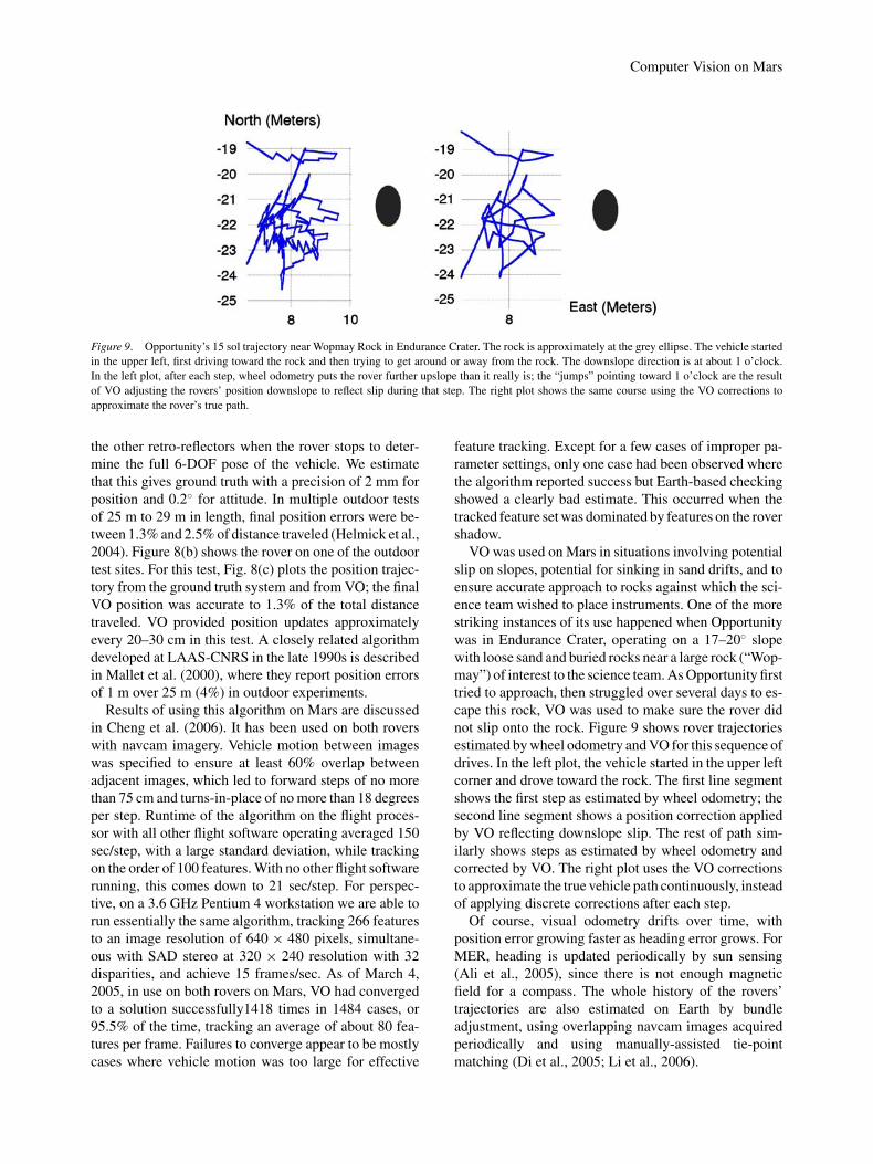
Figure 9. Opportunity’s 15 sol trajectory near Wopmay Rock in Endurance Crater. The rock is approximately at the grey ellipse. The vehicle started

in the upper left, first driving toward the rock and then trying to get around or away from the rock. The downslope direction is at about 1 o’clock.

In the left plot, after each step, wheel odometry puts the rover further upslope than it really is; the “jumps” pointing toward 1 o’clock are the result

of VO adjusting the rovers’ position downslope to reflect slip during that step. The right plot shows the same course using the VO corrections to

approximate the rover’s true path.

the other retro-reflectors when the rover stops to deter-mine the full 6-DOF pose of the vehicle. We estimatethat this gives ground truth with a precision of 2 mm forposition and 0.2◦ for attitude. In multiple outdoor testsof 25 m to 29 m in length, final position errors were be-tween 1.3% and 2.5% of distance traveled (Helmick et al.,2004). Figure 8(b) shows the rover on one of the outdoortest sites. For this test, Fig. 8(c) plots the position trajec-tory from the ground truth system and from VO; the finalVO position was accurate to 1.3% of the total distancetraveled. VO provided position updates approximatelyevery 20–30 cm in this test. A closely related algorithmdeveloped at LAAS-CNRS in the late 1990s is describedin Mallet et al. (2000), where they report position errorsof 1 m over 25 m (4%) in outdoor experiments.

Results of using this algorithm on Mars are discussedin Cheng et al. (2006). It has been used on both roverswith navcam imagery. Vehicle motion between imageswas specified to ensure at least 60% overlap betweenadjacent images, which led to forward steps of no morethan 75 cm and turns-in-place of no more than 18 degreesper step. Runtime of the algorithm on the flight proces-sor with all other flight software operating averaged 150sec/step, with a large standard deviation, while trackingon the order of 100 features. With no other flight softwarerunning, this comes down to 21 sec/step. For perspec-tive, on a 3.6 GHz Pentium 4 workstation we are able torun essentially the same algorithm, tracking 266 featuresto an image resolution of 640 × 480 pixels, simultane-ous with SAD stereo at 320 × 240 resolution with 32disparities, and achieve 15 frames/sec. As of March 4,2005, in use on both rovers on Mars, VO had convergedto a solution successfully1418 times in 1484 cases, or95.5% of the time, tracking an average of about 80 fea-tures per frame. Failures to converge appear to be mostlycases where vehicle motion was too large for effective

feature tracking. Except for a few cases of improper pa-rameter settings, only one case had been observed wherethe algorithm reported success but Earth-based checkingshowed a clearly bad estimate. This occurred when thetracked feature set was dominated by features on the rovershadow.

VO was used on Mars in situations involving potentialslip on slopes, potential for sinking in sand drifts, and toensure accurate approach to rocks against which the sci-ence team wished to place instruments. One of the morestriking instances of its use happened when Opportunitywas in Endurance Crater, operating on a 17–20◦ slopewith loose sand and buried rocks near a large rock (“Wop-may”) of interest to the science team. As Opportunity firsttried to approach, then struggled over several days to es-cape this rock, VO was used to make sure the rover didnot slip onto the rock. Figure 9 shows rover trajectoriesestimated by wheel odometry and VO for this sequence ofdrives. In the left plot, the vehicle started in the upper leftcorner and drove toward the rock. The first line segmentshows the first step as estimated by wheel odometry; thesecond line segment shows a position correction appliedby VO reflecting downslope slip. The rest of path sim-ilarly shows steps as estimated by wheel odometry andcorrected by VO. The right plot uses the VO correctionsto approximate the true vehicle path continuously, insteadof applying discrete corrections after each step.

Of course, visual odometry drifts over time, withposition error growing faster as heading error grows. ForMER, heading is updated periodically by sun sensing(Ali et al., 2005), since there is not enough magneticfield for a compass. The whole history of the rovers’trajectories are also estimated on Earth by bundleadjustment, using overlapping navcam images acquiredperiodically and using manually-assisted tie-pointmatching (Di et al., 2005; Li et al., 2006).

Matthies et al.

Algorithms for missions must reach a high degree ofmaturity several years before launch, so MER’s VO rep-resents fairly mature, tested software from the late 1990s.More recent research on VO has used other error func-tions and feature tracking methods with an emphasis onreal-time performance on Pentium architectures (Nisteret al., 2006). Motion estimation performance appears tobe comparable, though a direct comparison on commondata sets has not been made. Another more recent trend inthe literature has been the use of monocular or stereo im-age sequences in simultaneous localization and mapping(SLAM) problems, using Harris or SIFT and sometimesintegrating inertial sensors (Eustice et al., 2005; Se et al.,2002). Formulations for integration of multiple sensorsfor localization are definitely germane to rover naviga-tion. However, rover navigation is typically a one-waytraverse, whereas much research on SLAM and SIFTlandmarks addresses loop closure and contexts wherelandmarks might be revisited many times, so feature in-variance and path topology are less important for roversthan computational efficiency and the ability to achieveorder of 1% error in a linear traverse.

3.5. Overall Mars Navigation Results

Driving mode statistics through August 15, 2005, aregiven in Maimone et al. (2006). At that point, Spirit hadbeen on Mars for 573 sols and had driven 4798 m; Op-portunity had been on Mars for 555 sols and had driven5947 m. Spirit used stereo vision for obstacle detectionfor 28% of its total traverse and VO for 16%; obstacle de-tection and VO were only used together for 3 m, becausethat was too slow. Opportunity used stereo vision for ob-stacle detection for 21% of its traverse and VO for 11%;it never used obstacle detection and VO together. The restof the driving was commanded as “blind” drives, becauseoperators on Earth could see in navcam or pancam im-agery that the way was clear and chose to travel faster bynot incurring the runtime delay for the autonomous nav-igation functions. Spirit drove roughly 3 km on the floorof Gusev Crater to the base of the Columbia Hills, whichare about 100 m high, and has been in the hills ever since.Most of its obstacle detection was done on the floor ofthe crater, as part of drives in which an initial segmentthat operators could see was blind and beyond which ob-stacle detection was enabled. Most of its VO was donein the hills. Opportunity used obstacle detection duringvery long daily drives on the plains, mostly to avoid driv-ing into small craters. It used VO on sloping terrain inEagle Crater, Endurance Crater, and on the plains as itentered terrain with sand drifts, as a precaution againstgetting stuck with wheels spinning deeply in sand. As ofMarch 15, 2006, Spirit had covered 6797 m and Oppor-tunity 6645 m; driving mode statistics up to that point arenot yet available. Detailed narrations of driving experi-

ence for both rovers are given in Leger et al. (2005) andBiesiadeck et al. (2005).

Since the goal for the primary mission was to survive90 days and to drive a minimum of 600 m, the rovershave far surpassed that goal. Onboard computer visionalgorithms have been instrumental in that achievement.Moreover, because long drives were necessary to reachscientifically interesting terrain, MER has firmly estab-lished the importance of long range mobility for Marssurface exploration.

3.6. Lessons Learned

Before moving to a discussion of ongoing development,we will briefly recap key requirements for rover visionsystems and lessons learned from the MER mission.Rovers drive slowly and the terrain typically is not verycomplex, so lookahead distance requirements for obsta-cle detection are short. Power and energy are limited,which puts a premium on low-power electronics. Roverdriving is generally confined to a few hours around mid-day for operational reasons largely unrelated to the visionsystem. Simple, area-based feature tracking and stereocorrelation algorithms generally have proved sufficientfor velocity estimation for landers and for obstacle de-tection and visual odometry for rovers.

While MER has been a very successful mission despiteits slow computer, future missions will want to drive a lotfarther in a given amount of time, so faster implemen-tations of vision and planning algorithms are important.Several low-level data quality issues need to be addressedin stereo vision, including maximizing ability to matchin low-texture terrain such as that encountered at Merid-iani Planum and reducing pixel-locking artifacts. One ofthe key performance limitations in this mission has beenslip on slopes. Coping with this consumed a great dealof time when Opportunity was in Endurance Crater andprevented Opportunity from making a closer approachto scientifically interesting cliff outcrops in the crater.This could be improved by making visual odometry fastenough to use in a continuous steering control algorithmthat would compensate for slip.

4. Current Development

JPL is designing a new rover, called the Mars ScienceLaboratory (MSL), for the 2009 Mars launch window.This design is powered by a radio-isotope thermal gen-erator (RTG) instead of solar panels, is much larger thanMER, and is intended to be able to drive 20 km in a pri-mary mission of nearly two Earth years. Stereo camerasare again the sole 3-D perception sensors onboard. Theflight computer is a space-qualified PowerPC 750 with aclock rate of about 100 MHz; this brings floating point,


but still no L2 cache. Budget priorities dictate that MSL’sautonomous navigation capabilities will be little changedfrom MER. Nevertheless, vision system R&D is contin-uing along several lines in parallel to MSL development.This includes vastly increasing computational through-put by exploiting flight qualifiable field programmablegate arrays (FPGAs) as computing elements, improvingthe quality of disparity data by reducing noise, improv-ing performance at occluding boundaries, and reducingpixel locking, and attempting to learn to predict slippageahead of the vehicle by regressing past slippage experi-ence against the visual appearance of the terrain.

4.1. FPGA Computing

JPL is developing a new flight computing system, calledthe Mobility Avionics Module (MAM), around theXylinx Virtex-II Pro FPGA as the main computing ele-ment. This FPGA includes PowerPC 405 (PPC405) pro-cessor hard cores that can be clocked at up to 300 MHz;the rest of the FPGA logic can be clocked at approxi-mately 100 MHz. A prototype MAM exists as a PMCform factor (∼6 × 3 inch) board that weighs 150 g, draws3 W, and includes a Virtex II Pro with two embeddedPPC405 cores running Linux, with Ethernet, PCI bus,Compact Flash, 1394, and serial I/O. This board has beeninstalled in a research rover and the entire rover onboardsoftware has been ported to one PPC405 in the FPGA.Benchmarks show that stereo vision and VO run togetherin 6.4 sec/frame for 640 × 480 input imagery, 320 × 240disparity maps with 32 disparities, and VO tracking 266features in a four-level image pyramid. This is a vastspeed-up over the MER flight processor.

To increase speed further, we are moving the mosttime-consuming vision functions into the FPGA logic.Our initial step has been to move the SAD computationfor stereo vision into the logic, since that greatly domi-nates the runtime of the stereo algorithm. The logic im-plementation has been designed to be highly parallel andpipelined, so that in steady state it produces one subpixeldisparity estimate per clock cycle at a 100 MHz clockrate (Villalpando, 2006). The current implementation ishard-coded for 320 × 240 pixel imagery with 32 dispar-ities. SAD scores for all 32 disparities are computed inparallel, then flowed into a comparator tree that deter-mines the minimum SAD at each pixel and performsa left-right consistency check. Finally, subpixel dispar-ity is computed by parabolic fitting and output as 8 bitsof integer and 8 bits of subpixel data. The implementa-tion uses roughly 40% of the resources in a Virtex II Promodel 2VP4 FPGA. At one output pixel per clock cy-cle, the pipeline throughput rate is equivalent to roughly1 ms/frame. The current I/O implementation does not useDMA, so with I/O one frame takes 50 ms. Together with

running rectification, prefiltering, and triangulation onthe PPC405, the entire stereo process takes 250 ms/frame.

Related work on FPGA and other hardware-basedstereo implementations includes an FPGA implemen-tation of another SAD-based algorithm similar to ours([STOC] Stereo Head User Manual 1.1, 2006), a cus-tom ASIC implementation of the Census stereo algorithm(Woodfill et al., 2004), and an implementation of a multi-scale, multi-orientation, phase-correlation algorithm inmultiple FPGAs (Masrani and MacLean, 2006). The firsttwo are commercial products; all three claim speeds of30 Hz operation or greater on images of 512 × 480 or640 × 480 pixels. All of these are purely stereo machinesand do not include a general purpose processor core withan operating system that can host other application func-tions coded in C, as the FPGA in our mobility avionicsmodule does, so they were designed for more narrowpurposes. The key points to note about our work are that(1) it is becoming possible to fly high capacity FPGAsin space, including embedded microprocessors and largeamounts of reconfigurable logic in the same chip, and(2) such chips support area-based stereo in a few mil-liseconds/frame. A detailed, engineering-oriented com-parison of the chip real estate versus speed versus dispar-ity map quality of different real-time stereo algorithmswould be valuable, but is beyond our current scope.

4.2. Noise Reduction and Improved OccludingBoundaries

As engineering improvements, we are working to im-prove disparity estimation at rock boundaries and to im-prove the signal-to-noise ratio (SNR) of the disparitymaps, within the limits of real-time performance.

For better boundary estimation, we have had goodsuccess with using five overlapping SAD windows(“SAD5”) (Hirschmuller et al., 2002). In initial work ona real-time implementation, we have a SAD5 correlatorrunning at 30 Hz on a 1.4 GHz Pentium M for 320 × 240disparity maps and 32 disparities. We got further im-provement at occluding boundaries by changing the im-age prefiltering used to compensate for radiometric dif-ferences between left and right images. SAD is normallyrun on images that have been bandpass or highpass fil-tered to reduce brightness differences between the stereoimages, which arise from a number of causes. This fil-tering introduces overshoot or ringing artifacts at strongintensity edges. When such edges correspond to occlud-ing boundaries, the artifacts affect different parts of thebackground surface in the left and right images, whichcontributes to poor matching at occluding boundaries. Wehave addressed this by replacing linear filters with a fast,separable approximation to the edge-preserving bilateralfilter; that is, the bilateral-filtered image is subtracted

Matthies et al.

Figure 10. Stereo results on the same Spirit navcam imagery as Fig. 6, with SAD5 and improved low-level signal processing (see text). The occluding

boundary of the rock is cleaner, there are fewer holes in the disparity map, the small rocks are better delineated, the shadow to the right of the large

rock gets the disparity of the ground instead of the rock, and pixel-locking is slightly reduced.

from the original to reduce radiometric differences be-tween left and right images. Our experiments show thatthis produces better depth maps for a variety of outdoorscenes (Ansar et al., 2004).

In most of the research community, stereo evaluationhas focused on estimating integer disparity and scoringthe fraction of pixels with correct integer disparity. How-ever, for autonomous navigation applications, subpixelestimation is essential, so accuracy and precision of thesubpixel estimates is a key performance issue. This isaffected by such factors as aliasing caused by simpli-fications introduced to low-level filtering for real-timeperformance, pixel-locking, and other errors caused bycorrelation windows overlapping strong intensity edgesor occluding boundaries. In the MER stereo algorithm,aliasing arises from the use of bilinear interpolation inrectification and the use of block averaging in the high-pass filter used to compensate for radiometric differencesbetween images. We have not undertaken a detailed fre-quency domain analysis and redesign to address this, butwe have experimented with bicubic interpolation in rec-tification and better highpass filter kernels.

Figure 10 illustrates the effect on the MER HumphreyRock stereo pair of using bicubic interpolation in recti-fication, bilateral filtering for preprocessing, and SAD5for correlation (see Fig. 5 for comparison). The occlud-ing boundary of the rock is cleaner, there are fewer small

holes, the small rocks are better defined, and the shadowon the right edge of the rock gets the disparity of theground instead of the rock. Pixel-locking is also slightlyreduced, though this is hard to see in this figure; we ad-dress this in more detail in Section 4.3. To begin to quan-tify the difference, we have taken 10 left navcam imagesfrom Meridiani Planum, with appearances similar to por-tions of Fig. 4(b), shifted them to create synthetic rightimages with disparity gradients corresponding to a flatground plane seen from the navcam, and collected RMSdisparity error statistics for the stock MER algorithm andthe modified version described above. This yielded RMSerrors of 0.16 pixels and 0.09 pixels, respectively. Whilethis is just a start for quantitative evaluation, reducingthe noise in the disparity map by nearly a factor of twois significant for practical applications and indicates thatthis issue is worth further examination.

4.3. Reduced Pixel-Locking

We have recently conducted a short study of pixel-locking(Stein et al., 2006), the phenomenon in which disparitiesestimated by window-based stereo algorithms are biasedtoward integer disparities. It is desirable to reduce thiseffect in order to increase the feasible lookahead distancefor obstacle detection for a given stereo camera set-up.


Figure 11. Left image of a texture-mapped synthetic room and the corresponding ground truth disparity map. The blue lines are for visual aid only,

to help distinguish the surfaces in the room. The red dashed rectangles indicate the ceiling/floor regions used for analysis (see text). Also note that

any stair-stepped pattern visible in the disparity map is due to color quantization; the disparities do indeed vary smoothly.

This effect was noted at least as far back as Gennery(1980). Xiong explained it for SSD matching through afrequency domain analysis and showed modest improve-ment by replacing parabolic fits with quartic fits to es-timate subpixel disparity (Xiong and Matthies, 1997).Shimizu and Okutomi gave an analysis for both SSD andSAD matching and showed that SSD suffers less fromthis effect (Shimizu and Okutomi, 2001). Since the biasis approximately anti-symmetric around integer dispar-ity values, they proposed to reduce the effect by creat-ing new image pairs sampled halfway between the orig-inal pixels, doing subpixel stereo matching again withthe resampled imagery, and averaging the results withdisparities obtained from the original imagery. In theirexperiments, that reduced errors to 1/6 to 1/8 of the stan-dard method. Szeliski and Scharstein also analyzed SSDmatching in the frequency domain, though not with an ex-plicit focus on pixel-locking, and proposed stereo match-ing approaches based on interpolating imagery to higherresolution (Szeliski and Scharstein, 2002). Their algo-rithm had a number of complexities and was not targetedat real-time systems. The main conclusion of our study isthat iterative affine matching reduces the RMS disparityerror on planar surfaces and attenuates the rippling arti-facts from pixel-locking more than the Shimizu-Okutomimethod. The difference appears to increase with increas-ing surface tilt, which is both intuitive and significant forground vehicle navigation, where a steeply tilted groundsurface (relative to the camera frame) is the norm. Todate, we have not addressed runtime issues in this study,so prospects for real-time performance of iterative affinematching for subpixel stereo disparity estimation remainto be evaluated.

Our experiments used standard SAD stereo to estimateinteger disparities, then used affine matching constrained

to 1-D (along scanlines) to estimate subpixel disparity,allowing X translation, scale, and shear deformations ofthe template and iterating to convergence. This allowsinitial disparity errors of greater than one pixel to be cor-rected, which are quite possible in highly foreshortenedparts of the image. Standard parabola fitting cannot cor-rect errors greater than 0.5 pixels. The use of discretewindows for summing matching error required a fewadditional practical considerations. First, to avoid arti-facts due to sharp changes in matching cost as the win-dow’s size or position change, we used a Gaussian-shapedweighting function. In addition, we ignored any pixels(by zero-weighting them) which are marked as occludedor invalid in the initial integer disparity result. Finally,if the window straddles an occlusion boundary, the cen-ter pixel’s computed offset will be influenced by pixelsfrom a different physical surface in the image. Since wehave an initial estimate of disparity (and thus occlusionboundaries in the scene), we also ignore any pixels in thewindow whose initial integer disparity differs radicallyfrom that of the central pixel whose offset we are com-puting. To cope with local brightness differences betweenthe images, the matcher was applied after the differenceof bilateral filtering discussed earlier. For direct compar-ison to Shimizu-Okutomi, we used squared differencesinstead of absolute differences in the affine matcher. InStein et al. (2006), we referred to this method as “affineLK,” for affine Lucas-Kanade.

We compared this approach to simple parabola fit-ting and to our implementation of the error compen-sation scheme of Shimizu-Okutomi. To allow quantita-tive analysis, we first evaluated results on synthetic im-agery. The left image of a synthetic stereo pair along withthe corresponding ground truth disparity map are shownin Fig. 11, depicting a rectangular room with various

Matthies et al.

Figure 12. Histograms of subpixel disparity from the outlined region

on the ceiling of the synthetic room.

textures mapped to the planar ceiling, floor, and walls.Because the four surfaces in the room are planar, the truedistribution of subpixel disparities along each should beuniform. A histogram of ground truth subpixel disparitiesfor a region on the room’s ceiling is shown at the top ofFig. 12.

Initial integer disparities were computed for the pair asdescribed above. Windows for all results provided were7 × 7 pixels. After applying parabola fitting to estimatesubpixel disparity, we see in Fig. 12 the typical pixel-locking effect as peaks of subpixel disparity. Applyingthe approach of Shimizu and Okutomi (2001) improvesthe “peakiness” somewhat, and using Lucas-Kanade withwith constant windows yields similar results. But once weenable affine warping of the windows, we see the moredramatic flattening of the histogram shown at the bottomof the figure, which more closely resembles the groundtruth distribution. The floor region produces similarresults.

In addition to comparing disparity distributions, whichshed light on the pixel-locking performance, it is impor-tant to check the actual disparity errors as well. For theinitial integer disparity map shown in Fig. 13(a), considerits absolute error versus the ground truth disparity map,shown in Fig. 13(b). The errors have been capped at 0.5 tode-emphasize outliers and highlight initial smaller errors.Note that most of the errors on the floor start larger than0.5, which is most likely due to significant foreshorten-ing since the synthetic camera is placed fairly close to theground plane. The error maps after subpixel disparity es-timation by parabola fitting, by the approach in Shimizuand Okutomi (2001), and by the affine LK method areshown in Fig. 13(c)–(e), respectively. Note that errors onthe floor are significantly reduced only when using theaffine matcher.

Figure 14 compares the RMS error over the ceiling andfloor regions for the various approaches. To suppress theinfluence of outliers, we ignore all pixels whose initialinteger disparity error was greater than 3 when comput-ing the following RMS values (note that the choice ofthis threshold does not radically alter the results). For theceiling, both parabola fitting and the method in Shimizuand Okutomi (2001) do reduce the error from the initialinteger estimates by about 65%. The affine LK approachreduces the error by 78%. On the floor, where the errorsare much higher initially, both methods based on parabo-las yield only about 6% error reduction over the integerestimates, whereas the affine LK approach achieves 86%.

Figure 15 shows results on a real stereo image pair,taken from outdoor experiments in a field. We do nothave ground truth for this pair, but because the ground isroughly planar, we can expect a smooth distribution ofdisparity. The pixel-locking effect is clearly visible forsimple parabola fitting. The Shimizu-Okutomi methodshows a marked improvement for this pair, but the affineLK approach still produces the smoothest histogram.Figure 16 shows similar results on a difference imagepair.

Figure 17 shows oblique overhead views of 3-D recon-structions for portions of the scenes in Figs. 15 and 16.Pixel-locking ripples are clear in the parabola fitting re-sults and reduced in the Shimizu-Okutomi and affine LKresults. The 3-D reconstruction for the imagery in Fig. 16includes part of the nearest tree and the fallen log in thelower left corner of the image.

Overall, the affine LK approach produced results thatvaried from modestly to significantly better than theShimizu-Okutomi method, depending on surface tilt andother factors that were not controlled in these experi-ments. The affine LK approach adapts to the local slantof the underlying surface, which makes it appealing com-pared to simpler schemes like using a fixed, tilted horopterto rectify imagery before matching (Burt et al., 1995). Itis likely to reduce potential for false alarm obstacle de-tections on the ground. We have not yet tested the methodon uneven ground to ensure that true relief is preserved.Given that we still require a real-time implementation,the next phase of this work must weigh implementationcosts against the noise reduction realized for the variousapproaches to ameliorating pixel-locking.

4.4. Vision-Based Slip Prediction

One of the most significant mobility limitations to emergefrom MER is slippage on slopes. Using VO to improvestate estimation has already helped control steering tooffset slippage, but it would be valuable to be able topredict in advance when a slope might be slippery, so asto make more intelligent path planning decisions about


Figure 13. Absolute disparity errors for the synthetic room imagery, capped at 0.5. The large initial errors on the floor are corrected only using the

affine LK approach.

Figure 14. RMS subpixel disparity errors from the floor and ceiling regions of the synthetic room imagery.

Matthies et al.

Figure 15. The left image of a real stereo pair, initial integer disparity map, and subpixel disparity distributions for the ground region (yellow dashed

lines). The Shimizu-Okutomi method improves the results considerably, but affine LK does slightly better.

it. Attempting to predict slip from physical models ofwheel/soil interaction would be complex, particularlygiven the heterogeneity and spatial variation of real ter-rain surfaces and the unknown parameters of such mod-els that would have to be estimated first. Existing workon modeling wheel/soil interaction typically assumeshomogeneous terrain and simplifies the physical modelin addition (Andrade et al., 1998; Iagnemma et al., 2004).Therefore, we have begun to tackle slip prediction as avisual learning problem that, for the time being, avoidsmodeling wheel/soil interaction (Angelova, 2006a, b).

Our approach starts by building gridded elevation mapsof the terrain in front of the rover that record geometricand visual appearance features of the terrain. As the roverdrives over mapped areas, visual odometry is comparedto wheel odometry to estimate slip of the whole roveras a unit. Pairing the geometric and visual appearance

features (e.g. texture) of map cells with the measured slipin each cell enables learning a local, nonlinear regressionfunction that maps from the features to predicted roverslip. Since the input space of terrain features could be highdimensional, to limit the complexity of the problem wecurrently partition it as follows. We assume that terrainconsists of a number of distinct classes, where each classcan be recognized by visual features such as color andtexture, and we assume that slippage for each class is onlya function of slope. From labeled training data, we traina classifier to recognize the terrain class in each map cell;then for each class, we learn a regression function thatmaps from slope to slip.

To evaluate the feasibility of this approach, we first ex-perimented with predicting slip from slope for a single,known terrain class (Angelova et al., 2006a), then ex-tended our experiments to situations where the set of


Figure 16. The left image of a real stereo pair, initial integer disparity map, and subpixel disparity distributions for the ground region (yellow dashed

lines). Here the Shimizu-Okutomi method makes modest improvement and affine LK is again the smoothest.

classes and labeled training data were given (Angelovaet al., 2006b). Ultimately, our goal is to learn the set ofclasses from experience. However, a priori it was un-clear how well slip can be predicted from slope for evenjust one, known terrain class, so we tested this first, asfollows.

We estimate slope by fitting a plane to the average ele-vation of map cells in neighborhoods in front of the rover,and decompose slope into pitch and roll angles alignedwith the rover reference frame. We consider slip learn-ing as nonlinear function approximation. While manylearning algorithms can be applied to this problem, ourchoice is motivated by our goal to eventually have thealgorithm running onboard a rover with the ability to dofast, online updates. We selected a type of Receptive FieldRegression algorithm (Schaal and Atkeson, 1998) calledLocally Weighted Projection Regression (Vijayakumaret al., 2005). The main idea is to split the input domains

into sub-regions (called receptive fields), apply local lin-ear fits in each receptive field, and do weighted blendingof these to approximate a globally nonlinear function.

Slip S (as a function of terrain slopes x) can be writtenin the following form:

S(x) =C∑

c=1

e−‖x−xc‖2/λ

(bc

0 +R∑

r=1

bcr

⟨dc

r , x⟩)

where e−‖x−xc‖2/λ is a weighting function that dependson the distance from the query example x to the recep-tive field center xc, C is the number of receptive fieldsfor this dataset, bc

0, bcr , dc

r are the parameters of the lin-ear regression in each receptive field, and λ controls thereceptive field size and in our case is estimated using avalidation set (to avoid overfitting). Given the trainingdata D = {xi , Si }N

i=1, where the vector xi contains the

Matthies et al.

Figure 17. Oblique overhead views of the 3-D reconstructions from subpixel disparity maps for the imagery in Fig. 14 (left column) and Fig. 15

(right column), with camera viewing directions indicated by white arrorws.

estimated slopes from range imagery and Si are the cor-responding slip measurements at this particular location,the task of the learning procedure is to estimate the un-known parameters xc, bc

0, bcr , dc

r , λ so that they fit thetraining data D well (see Angelova et al., 2006a for de-tails). The receptive fields are distributed to cover theinput space so that all training data belong to at leastone receptive field. This is done by adding new recep-tive fields whenever an incoming training example is notcovered by other receptive fields. The linear fit in eachreceptive field is done using the Partial Least Squaresalgorithm (Wold, 1966), but other linear regression algo-rithms could be used (Schaal and Atkeson, 1998). Whena new point arrives, only the parameters of the receptivefields in the vicinity of this point are to be re-evaluated.This allows for fast update in online learning. Note thatthe assumed model for the function is fairly nonrestric-

tive and varieties of nonlinear behaviors could be learnedfrom the training data.

To test how well this works when the terrain type isknown, we acquired data with a testbed robotic vehicle infive different terrain types in a park next to JPL (soil, sand,gravel, asphalt, and woodchips). This represents a totalof about 5000 frames covering a total distance of about1 km, of which approximately 3000 frames were usedfor training and 2000 for testing. Figure 18 shows resultsfor one, representative terrain type (soil); results for theother types are discussed in Angelova et al. (2006a). Thevehicle was driven several times up and down the dirt hillshown in the inset photo; roughly half of this data wasused for training, the rest for testing. Comparing plotsof pitch (lower graphs) to slip (upper graphs), there is areasonable correlation between the two. RMS predictionerrors were 11.8% for the test data in this case. Results


0 200 400 600 800

0

50

100

Slip

X (

%)

Soil. Train. RMS:7.23%

0 200 400 600 800

0

10

20

Step number

Slo

pe

s (

de

g)

0 200 400 600 800

0

50

100

Soil. Test. RMS:11.8%

Slip [gnd truth]Slip [predicted]

0 200 400 600 800

0

10

20

Step number

Pitch

Roll

Figure 18. Learning to predict forward slip as a function of terrain slope: results for a single, known terrain type (soil). Top row shows predicted

(red) and ground truth (green) slip as a function of step number; training data is on the left, test data on the right. The bottom graphs show the

corresponding pitch and roll angles for each step number. Slip does correlate with pitch. Average RMS prediction error is given at the top of each

plot.

for other terrain types include RMS test errors of 3.6% onasphalt and 27.5% on gravel. Given the stochastic natureof slip and the presence of noise in various measurementsthat go into estimating slip, we consider these levels oferror to be encouraging. Note that Spirit has experiencedslippage has high as 125%; that is, it has actually slippedbackwards in the process of trying to climb.

In subsequent work with labeled training data for mul-tiple terrain types, we have used texton-based textureanalysis (Varma and Zisserman, 2005) for terrain clas-sification, then used slope as above for slip predictiononce the terrain class had been identified. Details and ex-perimental results are reported in Angelova et al. (2006b).The results to date are encouraging. As this still repre-sents early work on a new problem area, a number ofissues remain to be addressed, such as determining howwell the assumption of a discrete set of classes worksin Mars terrain, automatically learning the classes, andreducing this to a real-time, onboard system. Neverthe-less, we believe this foray into visual learning of terraintraversability properties is bearing fruit for Mars roversand will have impact on terrestrial applications of groundrobots as well.

5. Discussion and Future Directions

The MER mission has succeeded far beyond its primarymission objectives. The three computer vision algorithmsin the mission—stereo vision and visual odometry for the

rover and feature tracking for horizontal velocity estima-tion for the lander—have performed reliably and madematerial contributions to mission success. Limitations ofthe 20 MHz onboard processor kept these algorithms verysimple, but since this is the first time algorithms like thishave ever been used in a mission, this represents an impor-tant starting point and opens the door to more advancedalgorithms in future missions as onboard computing abil-ity improves.

The 100 MHz PowerPC 750 onboard computerplanned for a 2009 Mars rover now in design will im-prove the computing situation modestly. A much biggerboost may come from the use of FPGA-based computingin subsequent missions. JPL has prototyped a new com-puting system based on the Xylinx Virtex II Pro FPGA,with two embedded PowerPC 405 (PPC405) processorhard cores. Rover navigation software running on thePPC405s already shows dramatic speed improvementsover the MER computer. The stereo vision correlator hasbeen moved into the FPGA logic, with a throughput ofone pixel of disparity per clock cycle at 100 MHz, or theequivalent of about 1 ms for a 320 × 240 disparity mapwith 32 disparities. Additional functionality in the FPGAlogic will follow in the future.

We have discussed some efforts to improve the SNRof the disparity maps, improve disparity at occlud-ing boundaries, and reduce pixel-locking artifacts. TheSNR improvement and occluding boundary work is rela-tively mature and largely implementation-oriented in na-ture, though important for practical performance. Our

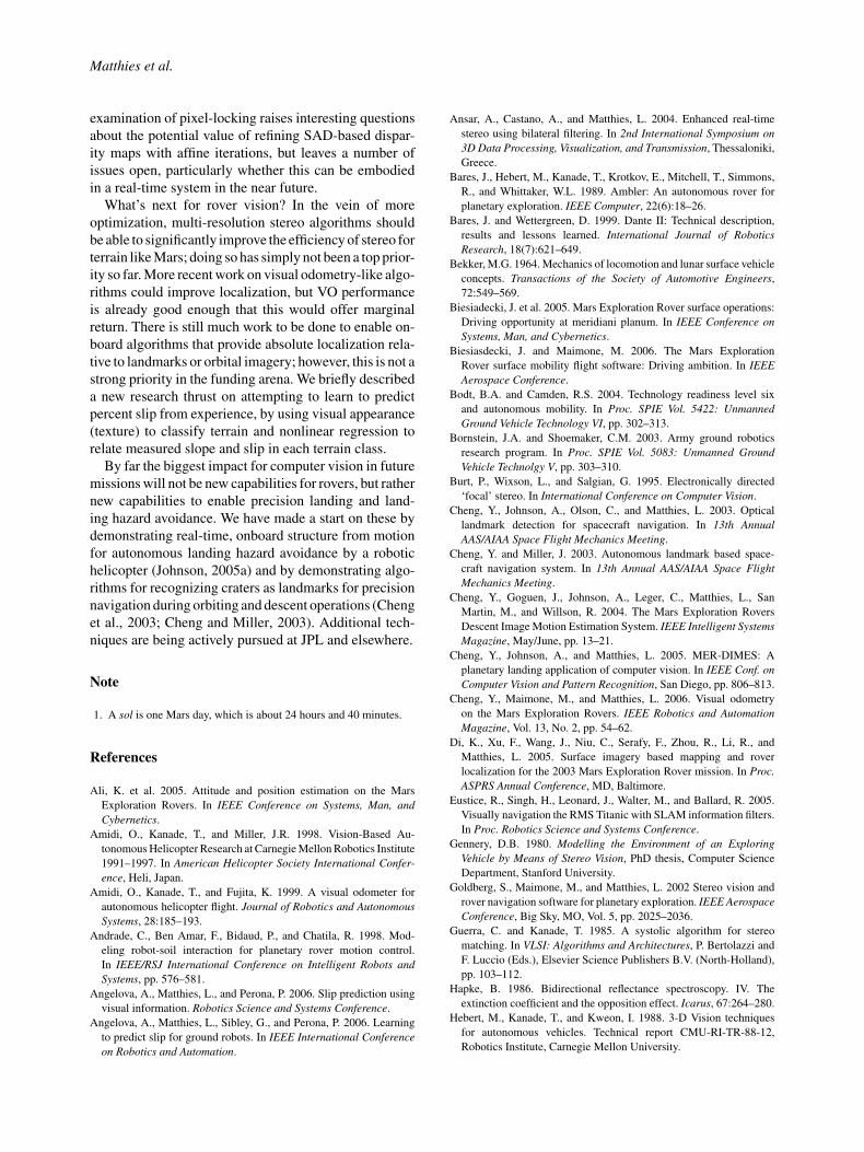
Matthies et al.

examination of pixel-locking raises interesting questionsabout the potential value of refining SAD-based dispar-ity maps with affine iterations, but leaves a number ofissues open, particularly whether this can be embodiedin a real-time system in the near future.

What’s next for rover vision? In the vein of moreoptimization, multi-resolution stereo algorithms shouldbe able to significantly improve the efficiency of stereo forterrain like Mars; doing so has simply not been a top prior-ity so far. More recent work on visual odometry-like algo-rithms could improve localization, but VO performanceis already good enough that this would offer marginalreturn. There is still much work to be done to enable on-board algorithms that provide absolute localization rela-tive to landmarks or orbital imagery; however, this is not astrong priority in the funding arena. We briefly describeda new research thrust on attempting to learn to predictpercent slip from experience, by using visual appearance(texture) to classify terrain and nonlinear regression torelate measured slope and slip in each terrain class.

By far the biggest impact for computer vision in futuremissions will not be new capabilities for rovers, but rathernew capabilities to enable precision landing and land-ing hazard avoidance. We have made a start on these bydemonstrating real-time, onboard structure from motionfor autonomous landing hazard avoidance by a robotichelicopter (Johnson, 2005a) and by demonstrating algo-rithms for recognizing craters as landmarks for precisionnavigation during orbiting and descent operations (Chenget al., 2003; Cheng and Miller, 2003). Additional tech-niques are being actively pursued at JPL and elsewhere.

Note

1. A sol is one Mars day, which is about 24 hours and 40 minutes.

References

Ali, K. et al. 2005. Attitude and position estimation on the Mars

Exploration Rovers. In IEEE Conference on Systems, Man, andCybernetics.

Amidi, O., Kanade, T., and Miller, J.R. 1998. Vision-Based Au-

tonomous Helicopter Research at Carnegie Mellon Robotics Institute

1991–1997. In American Helicopter Society International Confer-ence, Heli, Japan.

Amidi, O., Kanade, T., and Fujita, K. 1999. A visual odometer for

autonomous helicopter flight. Journal of Robotics and AutonomousSystems, 28:185–193.

Andrade, C., Ben Amar, F., Bidaud, P., and Chatila, R. 1998. Mod-

eling robot-soil interaction for planetary rover motion control.

In IEEE/RSJ International Conference on Intelligent Robots andSystems, pp. 576–581.

Angelova, A., Matthies, L., and Perona, P. 2006. Slip prediction using

visual information. Robotics Science and Systems Conference.

Angelova, A., Matthies, L., Sibley, G., and Perona, P. 2006. Learning

to predict slip for ground robots. In IEEE International Conferenceon Robotics and Automation.

Ansar, A., Castano, A., and Matthies, L. 2004. Enhanced real-time

stereo using bilateral filtering. In 2nd International Symposium on3D Data Processing, Visualization, and Transmission, Thessaloniki,

Greece.

Bares, J., Hebert, M., Kanade, T., Krotkov, E., Mitchell, T., Simmons,

R., and Whittaker, W.L. 1989. Ambler: An autonomous rover for

planetary exploration. IEEE Computer, 22(6):18–26.

Bares, J. and Wettergreen, D. 1999. Dante II: Technical description,

results and lessons learned. International Journal of RoboticsResearch, 18(7):621–649.

Bekker, M.G. 1964. Mechanics of locomotion and lunar surface vehicle

concepts. Transactions of the Society of Automotive Engineers,

72:549–569.

Biesiadecki, J. et al. 2005. Mars Exploration Rover surface operations:

Driving opportunity at meridiani planum. In IEEE Conference onSystems, Man, and Cybernetics.

Biesiasdecki, J. and Maimone, M. 2006. The Mars Exploration

Rover surface mobility flight software: Driving ambition. In IEEEAerospace Conference.

Bodt, B.A. and Camden, R.S. 2004. Technology readiness level six

and autonomous mobility. In Proc. SPIE Vol. 5422: UnmannedGround Vehicle Technology VI, pp. 302–313.

Bornstein, J.A. and Shoemaker, C.M. 2003. Army ground robotics

research program. In Proc. SPIE Vol. 5083: Unmanned GroundVehicle Technolgy V, pp. 303–310.

Burt, P., Wixson, L., and Salgian, G. 1995. Electronically directed

‘focal’ stereo. In International Conference on Computer Vision.

Cheng, Y., Johnson, A., Olson, C., and Matthies, L. 2003. Optical

landmark detection for spacecraft navigation. In 13th AnnualAAS/AIAA Space Flight Mechanics Meeting.

Cheng, Y. and Miller, J. 2003. Autonomous landmark based space-

craft navigation system. In 13th Annual AAS/AIAA Space FlightMechanics Meeting.

Cheng, Y., Goguen, J., Johnson, A., Leger, C., Matthies, L., San

Martin, M., and Willson, R. 2004. The Mars Exploration Rovers

Descent Image Motion Estimation System. IEEE Intelligent SystemsMagazine, May/June, pp. 13–21.

Cheng, Y., Johnson, A., and Matthies, L. 2005. MER-DIMES: A

planetary landing application of computer vision. In IEEE Conf. onComputer Vision and Pattern Recognition, San Diego, pp. 806–813.

Cheng, Y., Maimone, M., and Matthies, L. 2006. Visual odometry

on the Mars Exploration Rovers. IEEE Robotics and AutomationMagazine, Vol. 13, No. 2, pp. 54–62.

Di, K., Xu, F., Wang, J., Niu, C., Serafy, F., Zhou, R., Li, R., and

Matthies, L. 2005. Surface imagery based mapping and rover

localization for the 2003 Mars Exploration Rover mission. In Proc.ASPRS Annual Conference, MD, Baltimore.

Eustice, R., Singh, H., Leonard, J., Walter, M., and Ballard, R. 2005.

Visually navigation the RMS Titanic with SLAM information filters.

In Proc. Robotics Science and Systems Conference.

Gennery, D.B. 1980. Modelling the Environment of an ExploringVehicle by Means of Stereo Vision, PhD thesis, Computer Science

Department, Stanford University.

Goldberg, S., Maimone, M., and Matthies, L. 2002 Stereo vision and

rover navigation software for planetary exploration. IEEE AerospaceConference, Big Sky, MO, Vol. 5, pp. 2025–2036.

Guerra, C. and Kanade, T. 1985. A systolic algorithm for stereo

matching. In VLSI: Algorithms and Architectures, P. Bertolazzi and

F. Luccio (Eds.), Elsevier Science Publishers B.V. (North-Holland),

pp. 103–112.

Hapke, B. 1986. Bidirectional reflectance spectroscopy. IV. The

extinction coefficient and the opposition effect. Icarus, 67:264–280.

Hebert, M., Kanade, T., and Kweon, I. 1988. 3-D Vision techniques

for autonomous vehicles. Technical report CMU-RI-TR-88-12,

Robotics Institute, Carnegie Mellon University.


Hebert, M., Krotkov, E., and Kanade, T. 1989. A perception system

for a planetary rover. In Proc. 28th IEEE Conference on Decisionand Control, pp. 1151–1156.

Hebert, M., Bolles, B., Gothard, B., Matthies, L., and Rosenbloom,

M. 1996. Mobility for the unmanned ground vehicle. In Recon-naissance, Surveillance, and Target Recognition (RSTA) for theUnmanned Ground Vehicle, O. Firschein (Ed.), PRC Inc.

Helmick, D., Cheng, Y., Clouse, D., and Matthies, L. 2004. Path

following using visual odometry for a Mars Rover in high-slip

environments. In IEEE Aerospace Conference, Big Sky, MO.

Hirschmuller, H., Innocent, P.R., and Garibaldi, J. 2002. Real-

time correlation-based stereo vision with reduced border errors.

International Journal of Computer Vision, 47:229–246.

Iagnemma, K., Kang, S., Shibly, H., and Dubowsky, S. 2004. On-line

terrain parameter estimation for wheeled mobile robots with

application to planetary rovers. IEEE Transactions on Robotics,

20(5):921–927.

Johnson, A., Montgomery, J., and Matthies, L. 2005. Vision guided

landing of an autonomous helicopter in hazardous terrain. In IEEEInternational Conference on Robotics and Automation, Barcelona,

Spain.

Johnson, A., Willson, R., Goguen, J., Alexander, J., and Meller, D.

2005. Field testing of the Mars Exploration Rovers Descent Image

Motion Estimation System. In IEEE International Conference onRobotics and Automation, Barcelona, Spain, pp. 4463–4469.

Johnson, A., Willson, R., Cheng, Y., Goguen, J., Leger, C., SanMartin,

M., and Matthies, L. Design through operation of an image-based

velocity estimation system for Mars landing. Joint issue of the Inter-national Journal of Computer Vision and the International Journal ofRobotics Research, Special Issue on Vision and Robotics, to appear.

Kanade, T. and Ikeuchi, K. 1991. Introduction to the special issue

on physical modeling in computer vision. IEEE Transactions onPattern Analysis and Machine Intelligence, 13(7):609–610.

Kanade, T., Yoshida, A., Oda, K., Kano, H., and Tanaka, M. 1996.

A stereo machine for video-rate dense depth mapping and its new

applications. In Proc. IEEE Conf. on Computer Vision and PatternRecognition, pp. 196–202.

Kanade, T., Amidi, O., and Ke, Q. 2004. Real-time and 3D vision for

autonomous small and micro air vehicles. In IEEE Conference onDecision and Control.

Klinker, G., Shafer, S., and Kanade, T. 1990. A physical approach

to color image understanding. International Journal of ComputerVision, 4:7–38.

Konolige, K. 1997. Small vision systems: Hardware and implementa-

tion. In Proc. 8th International Symposium on Robotics Research,

Hayama, Japan.

Krotkov, E. and Simmons, R. 1996. Perception, planning, and

control for autonomous walking with the ambler planetary rover.

International Journal of Robotics Research, 15(2):155–180.

Krotkov, E. and Blitch, J. 1999. The DARPA tactical mobile

robotics program. International Journal of Robotics Research,

18(7):769–776.

Krotkov, E., Fish, S., Jackel, L., McBride, B., Pershbacher, M., and

Pippine, J. 2007. The DARPA PerceptOR evaluation experiments.

Autonomous Robots, to appear.

Leger, C. et al. 2005. Mars Exploration Rover surface operations:

driving Spirit at Gusev Crater. In IEEE Conference on Systems,Man, and Cybernetics.

Levine, M.D., O’Handley, D.A., and Yagi, G.M. 1973. Computer

determination of depth maps. Computer Graphics and ImageProcessing, 2:131–150.

Lewis, R.A. and Johnston, A.R. 1977. A scanning laser rangefinder for

a robotic vehicle. In Proc. 5th IJCAI, Cambridge, MA, pp. 762–768.

Li, R., Archinal, B., Arvidson, R., Bell, J., Christensen, P., Crumpler,

L., Des Marais, D., Di, K., Duxbury, T., Golombek, M., Grant, J.,

Greeley, R., Gunn, J., Johnson, A., Kirk, R., Maimone, M., Matthies,

L, Malin, M., Parker, T., Sims, M., Thompson, S., Squyres, S., and

Soderblom, L. 2006. Rover localization and topographic mapping

at the landing site of Gusev Crater, Mars. Journal of GeophysicalResearch—Planets, 111(E1).

Lindemann, R. and Voorhees, C. 2005. Mars Exploration Rover mo-

bility assembly design, test, and performance. In IEEE Conferenceon Systems, Man, and Cybernetics.

Maimone, M., Biesadecki, J., Tunstel, E., Cheng, Y., and Leger, C.

2006. Surface navigation and mobility intelligence on the Mars

Exploration Rovers. In Intelligence for Space Robotics, TSI Press,

Albuquerque, NM.

Maki, J. et al. 2003. Mars Exploration Rover engineering cameras.

Journal of Geophysical Research, 108(E12).

Mallet, A., Lacroix, S., and Gallo, L. 2000. Position estimation in out-

door environments using pixel tracking and stereovision. In IEEE In-ternational Conference on Robotics and Automation, pp. 3519–2524.

Masrani, D.K. and MacLean, W.J. 2006. A real-time large dispar-

ity range stereo-system using FPGAs. In Asian Conference onComputer Vision, Hyderabad, India.

Matthies, L. and Shafer, S, 1987. Error modelling in stereo navigation.

IEEE Journal of Robotics and Automation, RA-3(3).

Matthies, L. 1992. Stereo vision for planetary rovers: Stochastic

modeling to near real-time implementation. International Journalof Computer Vision, 8(1).

Matthies, L., Gat, E., Harrison, R., Wilcox, B., Volpe, R., and Litwin,

T. 1995. Mars microrover navigation: Performance evaluation and

enhancement. Autonomous Robots, 2(4).

Matthies, L., Kelly, A., Litwin, T., and Tharp, G. 1996. Obstacle

detection for unmanned ground vehicles: A progress report. In

Robotics Research: The Seventh International Symposium, G. Giralt

and G. Hirzinger (Eds.), Springer, pp. 475–486.

Matthies, L., Xiong, Y., Hogg, R., Zhu, D., Rankin, A., Kennedy, B.,

Hebert, M., Maclachlan, R., Won, C., and Frost, T. 2002. A portable,

autonomous, urban reconnaissance robot. Robotics and AutonomousSystems, 40(2).

Matthies, L. and Rankin, A. 2003. Negative obstacle detection by

thermal signature. In IEEE Conf. on Intelligent Robots and Systems,

Las Vegas, NV, pp. 906–913.

Matthies, L., Bellutta, P., and McHenry, M. 2003. Detecting water

hazards for autonomous off-road navigation. In SPIE Conf. onUnmanned Ground Vehicles, Orlando, FL.

Mettala, E.G. 1992. The OSD Tactical Unmanned Ground Vehi-

cle program. In Proc. DARPA Image Understanding Workshop,

MorganKaufmann Publishers, pp. 159–172.

Mettler, B., Tischler, M.B., and Kanade, T. 2001. System identification

modeling of a small-scale unmanned helicopter. Journal of theAmerican Helicopter Society.

Miller, J.R. and Amidi, O. 1998. 3-D Site mapping with the CMU au-

tonomous helicopter. In Proc. 5th International Conf. on IntelligentAutonomous Systems (IAS-5).

Montgomery, J., Johnson, A., Roumeliotis, S.I., and Matthies, L.

The JPL autonomous helicopter testbed: A platform for planetary

exploration technology research and development. Journal of FieldRobotics, to appear.

Moravec, H.P. 1980. Obstacle Avoidance and Navigation in the RealWorld by a Seeing Robot Rover, PhD thesis, Computer Science

Department, Stanford University.

Moravec, H.P. 1983. The Stanford Cart and the CMU Rover.

Proceedings of the IEEE, 71(7):872–884.

Nayar, S., Ikeuchi, K., and Kanade, T. 1991. Surface reflection:

Physical and geomerical perspectives. IEEE Transactions on PatternAnalysis and Machine Intelligence, 13(7):611–634.

Nister, D., Naroditsky, O., and Bergen, J. 2006. Visual odometry for

ground vehicle applications. Journal of Field Robotics, 23(1):3–

Matthies et al.

20.

A Scientific Rationale for Mobility in Planetary Environments. 1999.

Committee on Planetary and Lunar Exploration, National Research

Council. The National Academies Press.

Technology Development for Army Unmanned Ground Vehicles,

2002. Committee on Army Unmanned Ground Vehicle Technology,

Board on Army Science and Technology, Division of Engineering

and Physical Sciences, National Research Council, The National

Academies Press, Washington, D.C.

O’Handley, D.A. 1973. Scene analysis in support of a Mars Rover.

Computer Graphics and Image Processing, 2:281–297.

Okutomi, M. and Kanade, T. 1993. A multiple-baseline stereo.

IEEE Transactions on Pattern Analysis and Machine Intelligence,

15(4):353–363.

Pomerleau, D. and Jochem, T. 1996. Rapidly adapting machine vision

for automated vehicle steering. IEEE Expert: Special Issue onIntelligent Systems and their Applications, 11(2):19–27.

Schaal, S. and Atkeson, C. 1998. Constructive incremental learning

from only local information. Neural Computation, 10(8):2047–2084.

Se, S., Lowe, D., and Little, J. 2002. Mobile robot localization and

mapping with uncertainty using scale-invarianet visual landmarks.

International Journal of Robotics Research, 21(8).

Shimizu, M. and Okutomi, M. 2001. Precise sub-pixel estimation on

area-based matching. In International Conference on ComputerVision.

Shoemaker, C.M. and Bornstein, J.A. 2000. Overview and update of the

Demo III Experimental Unmanned Vehicle program. In Proc. SPIEVol. 4024: Unmanned Ground Vehicle Technology II, pp. 212–220.

Squyres, S. and Knoll, A.H. 2005. Sedimentary rocks at Meridiani

Planum: Origin, diagenesis, and implications for life on Mars.

Earth and Planetary Science Letters, Special Issue on Sedimentary

Geology at Meridiani Planum, Mars, Vol. 240, No. 1, pp. 1–10.

Stein, A., Huertas, A., and Matthies, L. 2006. Attenuating stereo

pixel-locking via affine window adaptation. In IEEE InternationalConference on Robotics and Automation.

Szeliski, R., and Scharstein, D. 2002. Symmetric sub-pixel stereo

matching. In European Conference on Computer Vision, pp.

525–540.

Thompson, A.M. 1977. The navigation system of the JPL robot. In

Proc. 5th IJCAI, Cambridge, MA, pp. 749–757.

Thorpe, C., Hebert, M., Kanade, T., and Shafer, S. 1991a. Toward

autonomous driving: The CMU Navlab. Part I: Perception. IEEEExpert, 6(4):31–42.

Thorpe, C., Hebert, M., Kanade, T., and Shafer, S. 1991b. Toward

autonomous driving: The CMU Navlab. Part II: System and

architecture. IEEE Expert, 6(4):44–52.

Thrun, S. 2001. A probabilistic online mapping algorithm for teams

of mobile robots. International Journal of Robotics Research,

20(5):335–363.

Tomasi, C. and Kanade, T. 1992. Shape and motion from image

streams under orthography: A factorization method. InternationalJournal of Computer Vision, 9(2):137–154.

Varma, M. and Zisserman, A. 2005. A statistical approach to texture

classification from single images. International Journal of ComputerVision, 62.

Stereo-on-a-Chip [STOC] Stereo Head User Manual 1.1, 2006. Videre

Design.

Vijayakumar, S., D’Souza, A., and Schaal, S. 2005. Incremen-

tal online learning in high dimensions. Neural Computation,

17(12):2602–2634.

Villalpando, C. 2006. Acceleration of stereo correlation in verilog. In

9th Military and Aerospace Programmable Logic Devices (MAPLD)International Conference, Washington, D.C.

Wettergreen, D., Thorpe, C., and Whittaker, W.L. 1993. Exploring

Mount Erebus by walking robot. Robotics and Autonomous Systems.

Wilcox, B.H. and Gennery, D.B. 1987. A Mars rover for the 1990s.

Journal of the British Interplanetary Society, pp. 483–488.

Wilcox, B. and Nguyen, T. 1998. Sojourner on Mars and lessons

learned for future planetary rovers. In Proc. 28th International Conf.on Environmental Systems (ICES’98), Danvers, MA, Society of

Automotive Engineers.

Williamson, T. 1998. A High-Performance Stereo Vision System forObstacle Detection, technical report CMU-RI-TR-98-24, Robotics

Institute, Carnegie Mellon University.

Willson, R., Johnson, A., and Goguen, D. 2005. MOC2DIMES: A

camera simulator for the Mars Exploration Rover Descent Image

Motion Estimation System. In 8th International Symposium onArtificial Intelligence, Robotics and Automation in Space (iSAIRAS),Munich, Germany.

Willson, R., Maimone, M., Johnson, A., and Scherr, L. 2005. An

optical model for image artifacts produced by dust particles on

lenses. In 8th International Symposium on Artificial Intelligence,Robotics, and Automation in Space (i-SAIRAS).

Wold, H. 1966. Estimation of principal components and related models

by iterative least squares. Multivariate Analysis, P.R. Krishnaiah

(Ed.), Academic Press, New York, pp. 391–420.

Woodfill, J., Gordon, G., and Buck, R. 2004. Tyzx DeepSea high speed

stereo vision system. In IEEE Workshop on Real Time 3-D Sensorsand their Use, Washington, D.C.

Xiong, Y. and Matthies, L. 1997. Error analysis of a real-time stereo

system. In IEEE Conference on Computer Vision and PatternRecognition, pp. 1087–1093.

Computer Vision on Mars Vision on Mars LARRY MATTHIES, MARK MAIMONE, ... 1992). This algorithm used...

Documents

Transcript of Computer Vision on Mars Vision on Mars LARRY MATTHIES, MARK MAIMONE, ... 1992). This algorithm used...