Computer Vision and Image Understanding 157 (2017) 103–116

Contents lists available at ScienceDirect

Computer Vision and Image Understanding

journal homepage: www.elsevier.com/locate/cviu

Modeling large-scale indoor scenes with rigid fragments using RGB-D

cameras

Diego Thomas a , b , ∗, Akihiro Sugimoto

c

a National Institute of Informatics, Tokyo 101-8430, Japan b Kyushu university, Fukuoka, Japan c National Institute of Informatics, Tokyo 101-8430, Japan

a r t i c l e i n f o

Article history:

Received 16 October 2015

Revised 10 August 2016

Accepted 29 November 2016

Available online 30 November 2016

Keywords:

3D Modeling

RGB-D Camera

Large-scale

Real-time

Loop closure

Bump image

Semi-global model

a b s t r a c t

Hand-held consumer depth cameras have become a commodity tool for constructing 3D models of in-

door environments in real time. Recently, many methods to fuse low quality depth images into a single

dense and high fidelity 3D model have been proposed. Nonetheless, dealing with large-scale scenes re-

mains a challenging problem. In particular, the accumulation of small errors due to imperfect camera

localization becomes crucial (at large scale) and results in dramatic deformations of the built 3D model.

These deformations have to be corrected whenever it is possible (when a loop exists for example). To

facilitate such correction, we use a structured 3D representation where points are clustered into several

planar patches that compose the scene. We then propose a two-stage framework to build in details and

in real-time a large-scale 3D model. The first stage (the local mapping) generates local structured 3D

models with rigidity constraints from short subsequences of RGB-D images. The second stage (the global

mapping) aggregates all local 3D models into a single global model in a geometrically consistent manner.

Minimizing deformations of the global model reduces to re-positioning the planar patches of the local

models thanks to our structured 3D representation. This allows efficient, yet accurate computations. Our

experiments using real data confirm the effectiveness of our proposed method.

© 2016 Elsevier Inc. All rights reserved.

1

e

M

m

h

i

c

s

m

g

d

v

p

s

h

S

(

s

c

r

v

e

t

b

v

c

a

s

C

o

f

q

e

h

1

. Introduction

3D reconstruction of indoor scenes using consumer depth cam-

ras has attracted an ever-growing interest in the last decade.

any applications such as robot navigation, virtual and aug-

ented reality or digitization of cultural heritage can benefit from

ighly detailed large-scale 3D models of indoor scenes built us-

ng cheap RGB-D sensors. In general, the 3D reconstruction pro-

ess consists of (1) generating multiple 2.5D views of the target

cene, (2) registering (i.e., aligning) all different views into a com-

on coordinate system, (3) fusing all measurements into a sin-

le mathematical 3D representation and (4) correcting possible

eformations.

To obtain depth measurements of a target scene (i.e., 2.5D

iews), many strategies exist, which can be classified into either

assive sensing or active sensing. A popular example for pas-

ive sensing is stereo vision ( Lazaros et al., 2008 ). On the other

and, structured light ( Rusinkiewicz et al., 2002 ) and time-of-flight

∗ Corresponding author at: Kyushu University, Motooka, Fukuoka 819-0395, Japan.

E-mail addresses: diegot.thomas@gmail.com (D. Thomas), sugimoto@nii.ac.jp (A.

ugimoto).

c

l

u

s

ttp://dx.doi.org/10.1016/j.cviu.2016.11.008

077-3142/© 2016 Elsevier Inc. All rights reserved.

Hansard et al., 2012 ) are the most popular techniques for active

ensing. Consumer depth cameras such as the Microsoft Kinect

amera or the Asus Xtion pro camera use such techniques and are

ecent active sensors which produce low quality depth images at

ideo rate and at low cost. These sensors have raised much inter-

st in the computer vision community, and in particular for the

ask of automatic 3D modeling.

The video frame rate provided by consumer depth cameras

rings several advantages for 3D modeling. One distinguished ad-

antage is that it simplifies the registration problem. This is be-

ause the transformation between two successive frames can be

ssumed to be sufficiently small. As a consequence, well-known

tandard registration algorithms such as variants of the Iterative

losest Point (ICP) ( Besl and McKay, 1992 ) work efficiently. More-

ver, by accumulating many (noisy) depth measurements available

or each point in the scene, it is possible to compensate for the low

uality of a single depth image and construct detailed 3D mod-

ls. A well known successful work for 3D modeling using RGB-D

ameras is KinectFusion ( Newcombe et al., 2011 ). In this system, a

inearized version of Generalized ICP (GICP) ( Segal et al., 2009 ) is

sed in the frame-to-global-model registration framework to align

uccessive depth images, which are accumulated into a volumet-

104 D. Thomas, A. Sugimoto / Computer Vision and Image Understanding 157 (2017) 103–116

i

b

e

m

c

i

b

a

s

e

a

a

p

m

a

u

s

s

2

R

m

t

c

p

u

c

(

(

s

t

i

d

m

m

q

n

t

l

t

t

c

a

p

t

i

r

o

d

p

w

t

s

K

t

a

i

d

a

3

t

t

i

ric Truncated Signed Distance Function (TSDF) ( Curless and Levoy,

1996 ) using a running average. With using rather simple, well-

established tools, impressive 3D models at video frame rate can

be obtained, which demonstrates the potential of RGB-D cameras

for fine 3D modeling.

Another new interesting property of consumer depth cameras

is that they can be held by hands and thus they allow reconstruct-

ing large-scale scenes rather easily. With this new possibility, new

challenges also arise: how to deal with error propagation and a

large amount of data? In other words, how to minimize deforma-

tions of the produced 3D model while keeping fine details, even at

large-scale?

In the last several years, a lot of research have been reported

to allow large-scale 3D reconstruction ( Chen et al., 2013; Henry

et al., 2013; Meilland and Comport, 2013; Neibner et al., 2013; Roth

and Vona, 2012; Thomas and Sugimoto, 2014 ; Whelan et al., 2012 ;

Zeng et al., 2013; Zhou and Koltun, 2013; Zhou et al., 2013 ). No-

ticeable works employ hash tables for efficient storage of volumet-

ric data ( Neibner et al., 2013 ), patch volumes to close loops on the

fly ( Henry et al., 2013 ) and non-rigid registration of sub-models to

reduce deformations ( Zhou et al., 2013 ). Though recent works con-

siderably improved the scale and the quality of 3D reconstruction

using consumer depth cameras, existing methods still suffer from

little flexibility for manipulating the constructed 3D models. This

is because most of existing methods work at the pixel level with

unstructured 3D representations (voxels with volumetric TSDF or

3D vertices with meshes). Modifying the whole 3D model then

becomes difficult and computationally expensive, which precludes

from closing loops or correcting deformations on-the-fly. Instead of

unstructured representations, introducing the structured 3D rep-

resentation overcomes this problem. In the work by Henry et al.

(2013) , indeed, patch volumes are used to manipulate structured

3D models, which allows simpler modifications of the 3D model.

In this work, we push forward in this direction by taking advan-

tage of a parametric 3D surface representation with bump im-

age ( Thomas and Sugimoto, 2013 ) that allows easy manipulations

of the 3D model while maintaining fine details, real-time perfor-

mance and efficient storage. Our experimental evaluation demon-

strates that by using the structured 3D representation, loops can

be efficiently closed on-the-fly and overall deformations are kept

to a minimum, even for large-scale scenes.

The main contributions of this paper are: (1) the creation of a

semi-global model to locally fuse depth measurements and (2) the

introduction to identity constraints between multiple instances of

a same part of the scene viewed at different time in the RGB-D

image sequence, which enables us to run a fragment registration

algorithm to efficiently close loops. Overall, we propose a method

that segments the input sequence of RGB-D images both in time

and space and that is able to build in real-time high fidelity 3D

models of indoor scenes. After briefly recalling the parametric 3D

surface representation with bump image in Section 3 we introduce

our two-stage strategy in Section 4 . We demonstrate the effective-

ness of our proposed method through comparative evaluation in

Section 5 before concluding in Section 6 . We note that a part of

this work appeared in Thomas and Sugimoto (2014) .

2. Related work

In the last few years, much work has been proposed to fuse

input RGB-D data into a common single global 3D model.

Weise et al. (2009) proposed to build a global 3D model us-

ing surface elements called Surfels ( Pfister et al., 20 0 0 ). They also

proposed to handle loop closure by enforcing the global model as-

rigidly-as-possible using a topology graph where each vertex is a

Surfel and edges connect neighboring Surfels. However, maintain-

ng such a topology graph for large-scale scenes is not practical

ecause of the existence of potentially millions of Surfels. Keller

t al. (2013) proposed a real-time point-based fusion algorithm for

emory efficient and robust 3D reconstruction. However, how to

orrect drift errors that arise at large scale is not discussed, which

s a crucial limitation when reconstructing large scale scenes.

Newcombe et al. (2011) proposed KinectFusion: a system to

uild implicit 3D representations of a scene from an RGB-D camera

t an interactive frame-rate (higher than 30fps). The implicit repre-

entation consists of a TSDF that is discretized into a volume cov-

ring the scene to be reconstructed. From the volumetric TSDF and

given camera pose, dense depth images can be generated, which

llows accurate and robust camera pose tracking. They also pro-

osed a GPU framework to integrate live depth data into the volu-

etric TSDF at interactive frame-rate. The TSDF is recorded into

regular voxel grid, which requires a large amount of memory

sage. This limits the practicability of the method for large-scale

cenes.

Thereafter, much work has been done on extending KinectFu-

ion for large-scale applications ( Chen et al., 2013; Neibner et al.,

013; Roth and Vona, 2012 ; Whelan et al., 2012 ; Zeng et al., 2013 ).

oth and Vona (2012) and Whelan et al. (2012) proposed Kinect

oving volumes and Kintinuous (respectively). In these methods,

he volume is automatically translated and rotated in space as the

amera moves, and remapped into a new one by the TSDF inter-

olation whenever sufficient camera movement is observed. The

se of the non-regular volumetric grid has also been studied for

ompact TSDF representations. Zeng et al. (2013) and Chen et al.

2013) proposed an octree-based fusion method. Neibner et al.

2013) proposed to use hash tables to achieve significant compres-

ion of the volumetric TSDF. However, because of the accumula-

ion of errors generated when registering and integrating incom-

ng RGB-D data, the global volumetric TSDF inevitably becomes

eformed when applied to a large-scale scene. Correcting defor-

ations in the volumetric TSDF is tedious and, as a consequence,

ultiple passes over the whole sequence of RGB-D images are re-

uired. This also means that the whole sequence of RGB-D images

eeds to be recorded at run-time. This becomes a critical limita-

ion for large-scale applications.

Meilland and Comport (2013) proposed a method to reconstruct

arge-scale scenes by using an image-based keyframe method. Mul-

iple keyframes are recorded along the camera path and merged

ogether to produce RGB-D images from any viewpoint along the

amera path that can be used for robust camera tracking or visu-

lization. Once the whole image sequence is processed, a cloud of

oint or a mesh is generated by running a voxel-based reconstruc-

ion algorithm over the set of keyframes. Loops may be closed us-

ng keyframes, and drifts in the estimated camera pose can be cor-

ected accordingly. However, uniformly redistributing drift errors

ver the camera path is not reasonable at large scale because the

istribution of the errors is, in general, not uniform.

Zhou and Koltun (2013) proposed to use local volumes around

oints of interest, and proposed an offline reconstruction method

ith two passes. The first pass estimates a rough camera trajec-

ory and segment the camera path into interest and connector

egments. The second pass refines the camera path by employing

inectFusion in each interest segment. A pose-graph is built during

he second pass that is optimized in a post-process for the final

ccurate estimation of the camera trajectory. Thereafter all RGB-D

mages are fused into a large volumetric TSDF (computation are

one on CPU so that memory is not a problem anymore) to gener-

te the final 3D model. The proposed technique allows for accurate

D modeling of large-scale scenes but at the cost of huge compu-

ational time. Moreover, as pointed out in Zhou et al. (2013) , even

he ground truth camera trajectory is not sufficient to generate the

deal 3D model. This is because of the low frequency noise that

D. Thomas, A. Sugimoto / Computer Vision and Image Understanding 157 (2017) 103–116 105

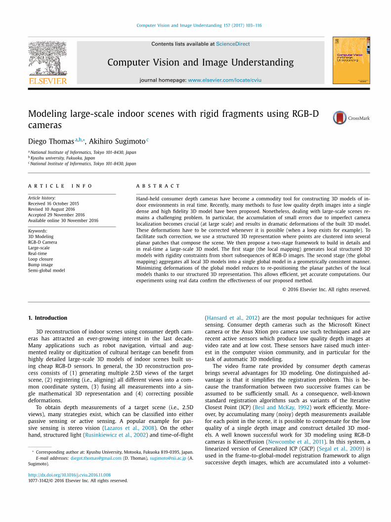
Fig. 1. The 3D representation for an indoor scene. The target scene is segmented

into multiple coplanar parts. Each segment S is modeled by the equation of the

plane P that best fit the set of 3D points in S , the 2D bounding box of the projec-

tion of all 3D points in S into the plane P , and three 2D images that encode local

geometry (Bump), color (Color) and confidence of measurements (Mask). (For inter-

pretation of the references to color in this figure legend, the reader is referred to

the web version of this article.)

e

t

Z

3

a

t

e

t

o

a

a

e

t

a

p

t

f

a

W

b

c

b

a

a

A

m

a

c

f

c

i

w

a

o

t

i

s

m

3

s

i

s

o

i

b

l

r

r

g

T

r

r

m

p

r

w

2

a

c

i

i

e

3

p

a

F

3

w

s

d

t

r

�

o

π

π

c

W

1

3

r

1 n is the normal of the plane � and d is the distance of the plane � from the

origin. 2 The notation [[ a, b ]] denotes the integer interval between a and b .

xists in each depth image (such noise may come from lens distor-

ion or inexact camera models for example).

To account for the low frequency noise in each depth image,

hou et al. (2013) proposed to employ elastic registration between

D meshes built from short subsequences of the whole RGB-D im-

ge sequence. The KinectFusion algorithm is applied to each short-

ime subsequence and then local meshes of the scene are gen-

rated. After all subsequences are processed, an elastic registra-

ion algorithm runs that combines rigid alignment and non-rigid

ptimization for accurate alignment, and correction of drift-errors

nd distortions caused by the low frequency noise. This method

chieves the state-of-the-art accuracy in 3D reconstruction. How-

ver, the computational cost is expensive and the elastic registra-

ion is a post-process, which prevents the method from real-time

pplications.

Henry et al. (2013) proposed to segment the scene into planar

atches and to use 3D TSDF volumes around them to represent

he 3D scene. In Henry et al. (2013) , a pose-graph optimization

or loop closure was proposed where each vertex of the graph is

planar patch and it is connected to one or multiple keyframe(s).

hen a loop is detected, it gives constraints on the relationship

etween patches and keyframes. Optimizing the graph to meet the

onstraints reduces deformations. When the 3D scene represented

y old patches is deformed due to drift errors, however, the rigid

lignment is not reliable anymore. Moreover, a critical question

bout when to merge overlapping patches in a loop is left open.

lso, the processing time drops drastically due to procedures for

aintaining planar patches. In Thomas and Sugimoto (2013) , the

uthors proposed a method that requires only three 2D images,

alled attributes (i.e., Bump image, Mask image and Color image),

or each planar patch to model the scene, which allows a more

ompact representation of the scene. Though they achieved signif-

cant compression of the 3D scene representation, no discussion

as given about how to deal with deformations that arise when

pplied to large-scale scenes.

Differently from the above methods, this paper uses the graph

ptimization framework with new rigidity constraints built be-

ween planar patches representing different parts of the scene and

dentity constraints built between planar patches representing the

ame part of the scene to accurately and efficiently correct defor-

ations of the global model. ( Figs. 1–14 ).

. Parametric 3D scene representation

We construct 3D models of indoor scenes using a structured 3D

cene representation based on planar patches augmented by Bump

mages ( Thomas and Sugimoto, 2013 ). At run-time, the scene is

egmented into multiple planar patches and the detailed geometry

f the scene around each planar patch is recorded into the Bump

mages. Each Bump image (i.e., the local geometry) is assumed to

e accurate because standard RGB-D SLAM algorithms work well

ocally (deformation problems arise at large scale). Therefore, cor-

ecting deformations at large scale in our built 3D model can be

educed to repositioning each planar patch consistently (the local

eometry encoded in the Bump image do not need to be modified).

his allows efficient computations. We choose to use the paramet-

ic representation with Bump image ( Thomas and Sugimoto, 2013 )

ather than patch volumes ( Henry et al., 2013 ) because (1) it is a

ore compact representation and (2) it is easier to compute dense

oint correspondences between multiple planar patches, which is

equired to run accurate registration (see Section 4.2.2 ). Below,

e briefly review our used representation ( Thomas and Sugimoto,

013 ) to make the paper self-contained.

To each surface patch detected in the scene, three 2D images

re attached as its attributes: a three-channel Bump image, an one-

hannel Mask image and a three-channel Color image. These three

mages encode geometric and color details of the scene. The Bump

mage encodes the local geometry around the planar patch. For

ach pixel, we record in the three channels the displacement of the

D point position from the lower left-corner of its corresponding

ixel. The Mask image encodes the confidence of accumulated data

t a point and the Color image encodes the color of each point.

ig. 1 illustrates the 3D representation for an indoor scene.

.1. Planar patches with attributes

Let us assume we are given a set of points P = { p 1 , p 2 , . . . , p n }ith n > 2 and there are at least 3 points that do not lie on the

ame line, and a planar patch � of a finite size, with the equation

etermined by ( n , d ) 1 and 2D bounding box Bbox = (l l , l r, ul , ur)

hat best fits P . Any 3D point on � (with normal n ) can be rep-

esented using parameters ( t, h ) with 0 ≤ t, h ≤ 1 that run over

.

� : ([0 , 1]) 2 → R

3

(t, h ) � −→ (x (t, h ) , y (t, h ) , z(t, h )) � .

Computation of the projected points. We define a projection

perator π� for �, such that for any p ∈ R

3 ,

�(p ) = argmin

(t,h ) ∈ ([0 , 1]) 2 (‖ p − �(t, h ) ‖ 2 ) .

�( p ) represents the 2D parameters of the projection of p onto �.

Discretisation of the planar patch. The planar patch � is dis-

retized in both dimensions into given m and l uniform segments.

e define the operator discr that maps real coordinates ( t, h ) ∈ ([0,

]) 2 into discrete coordinates 2 discr ( t, h ) ∈ [[0, m ]] × [[0, l ]].

∀ (t, h ) ∈ ([0 , 1]) 2 , discr(t, h ) = ( t × m � , h × l� ) .

.2. Bump image

The Bump image, encoded as a three-channel 16 bits image,

epresents the local geometry of the scene around a planar patch.

106 D. Thomas, A. Sugimoto / Computer Vision and Image Understanding 157 (2017) 103–116

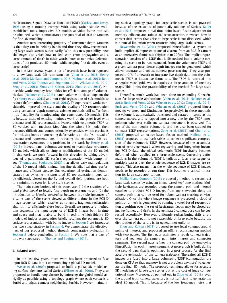
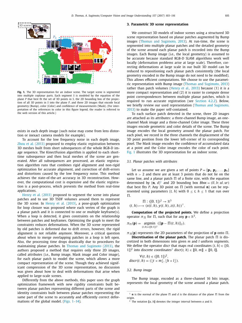
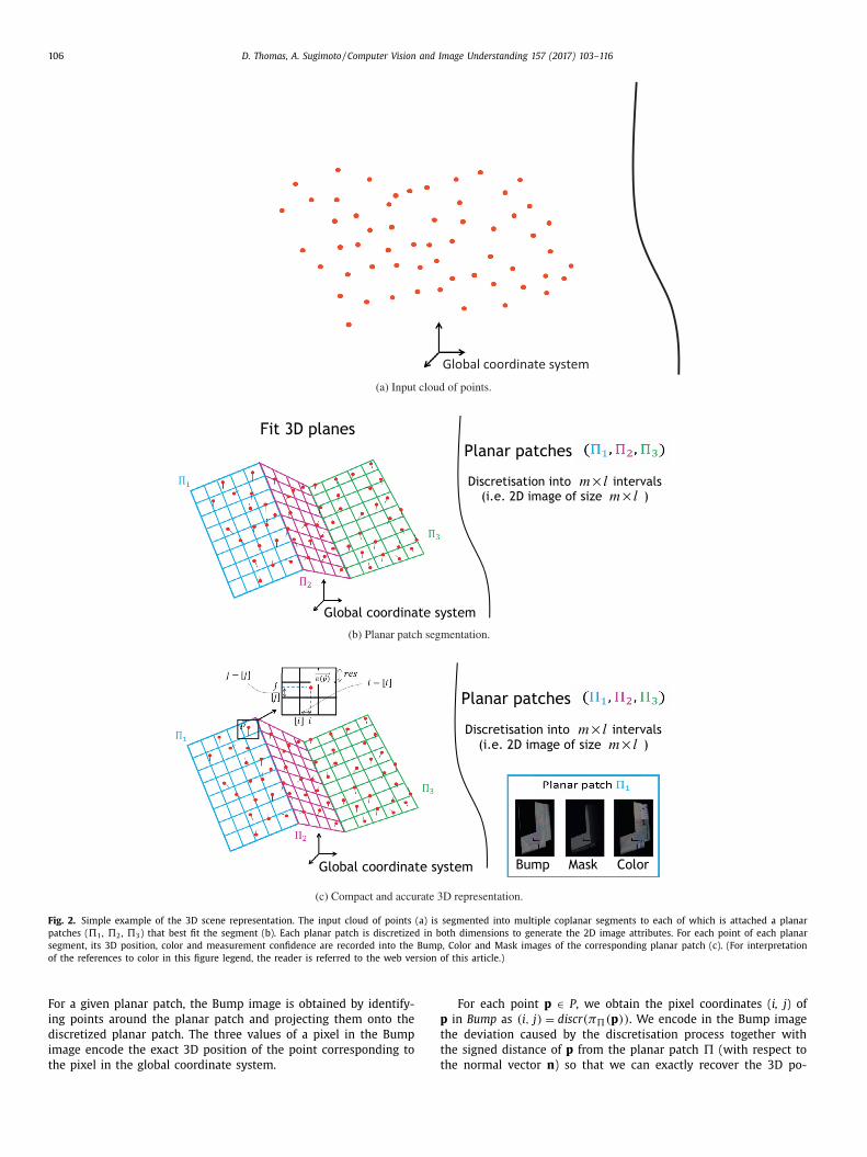
Fig. 2. Simple example of the 3D scene representation. The input cloud of points (a) is segmented into multiple coplanar segments to each of which is attached a planar

patches ( �1 , �2 , �3 ) that best fit the segment (b). Each planar patch is discretized in both dimensions to generate the 2D image attributes. For each point of each planar

segment, its 3D position, color and measurement confidence are recorded into the Bump, Color and Mask images of the corresponding planar patch (c). (For interpretation

of the references to color in this figure legend, the reader is referred to the web version of this article.)

p

t

t

t

For a given planar patch, the Bump image is obtained by identify-

ing points around the planar patch and projecting them onto the

discretized planar patch. The three values of a pixel in the Bump

image encode the exact 3D position of the point corresponding to

the pixel in the global coordinate system.

For each point p ∈ P , we obtain the pixel coordinates ( i, j ) of

in Bump as (i, j) = discr(π�(p )) . We encode in the Bump image

he deviation caused by the discretisation process together with

he signed distance of p from the planar patch � (with respect to

he normal vector n ) so that we can exactly recover the 3D po-

D. Thomas, A. Sugimoto / Computer Vision and Image Understanding 157 (2017) 103–116 107

s

t

B

t

s

w

p

p

u

a

c

N

n

H

p

a

c

s

3

l

m

o

A

t

T

p

R

p

3

4

c

t

t

r

r

s

c

p

p

s

r

i

s

1

p

(

s

m

b

c

n

r

k

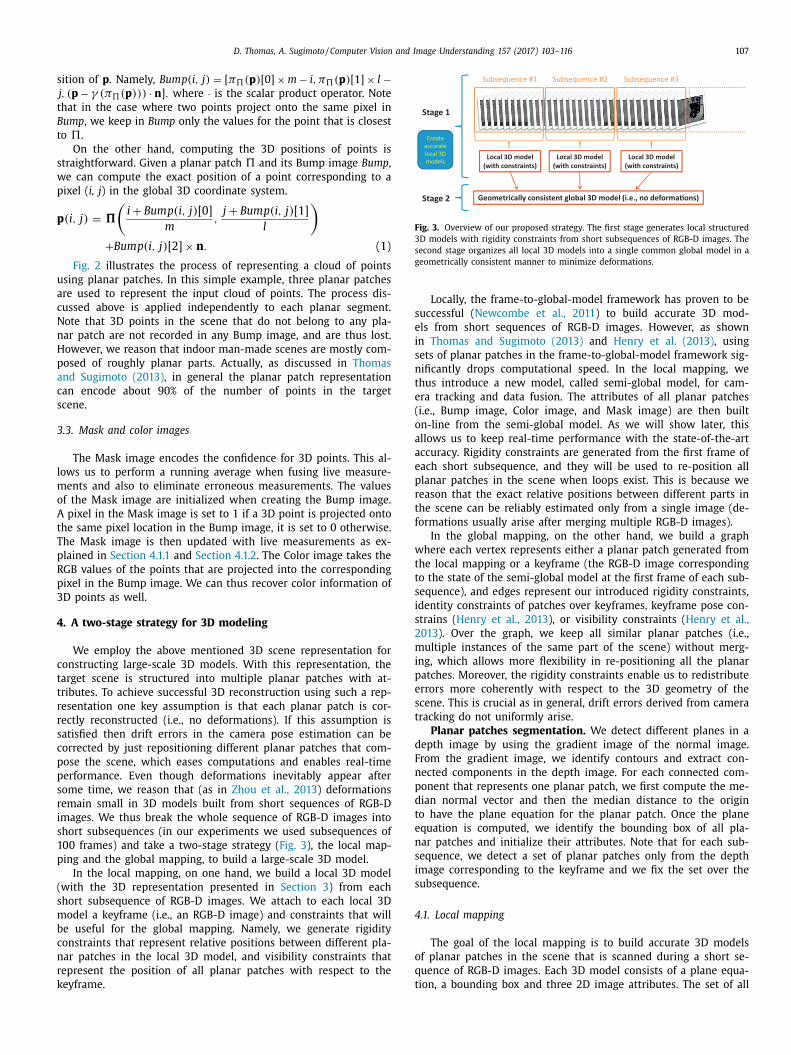
Fig. 3. Overview of our proposed strategy. The first stage generates local structured

3D models with rigidity constraints from short subsequences of RGB-D images. The

second stage organizes all local 3D models into a single common global model in a

geometrically consistent manner to minimize deformations.

s

e

i

s

n

t

e

(

o

a

a

e

p

r

t

f

w

t

t

s

i

s

2

m

i

p

e

s

t

d

F

n

p

d

t

e

n

s

i

s

4

o

q

t

ition of p . Namely, Bump(i, j) = [ π�(p )[0] × m − i, π�(p )[1] × l −j, (p − γ (π�(p ))) · n ] , where · is the scalar product operator. Note

hat in the case where two points project onto the same pixel in

ump , we keep in Bump only the values for the point that is closest

o �.

On the other hand, computing the 3D positions of points is

traightforward. Given a planar patch � and its Bump image Bump ,

e can compute the exact position of a point corresponding to a

ixel ( i, j ) in the global 3D coordinate system.

(i, j) = �

(i + Bump(i, j)[0]

m

, j + Bump(i, j)[1]

l

)

+ Bump(i, j)[2] × n . (1)

Fig. 2 illustrates the process of representing a cloud of points

sing planar patches. In this simple example, three planar patches

re used to represent the input cloud of points. The process dis-

ussed above is applied independently to each planar segment.

ote that 3D points in the scene that do not belong to any pla-

ar patch are not recorded in any Bump image, and are thus lost.

owever, we reason that indoor man-made scenes are mostly com-

osed of roughly planar parts. Actually, as discussed in Thomas

nd Sugimoto (2013) , in general the planar patch representation

an encode about 90% of the number of points in the target

cene.

.3. Mask and color images

The Mask image encodes the confidence for 3D points. This al-

ows us to perform a running average when fusing live measure-

ents and also to eliminate erroneous measurements. The values

f the Mask image are initialized when creating the Bump image.

pixel in the Mask image is set to 1 if a 3D point is projected onto

he same pixel location in the Bump image, it is set to 0 otherwise.

he Mask image is then updated with live measurements as ex-

lained in Section 4.1.1 and Section 4.1.2 . The Color image takes the

GB values of the points that are projected into the corresponding

ixel in the Bump image. We can thus recover color information of

D points as well.

. A two-stage strategy for 3D modeling

We employ the above mentioned 3D scene representation for

onstructing large-scale 3D models. With this representation, the

arget scene is structured into multiple planar patches with at-

ributes. To achieve successful 3D reconstruction using such a rep-

esentation one key assumption is that each planar patch is cor-

ectly reconstructed (i.e., no deformations). If this assumption is

atisfied then drift errors in the camera pose estimation can be

orrected by just repositioning different planar patches that com-

ose the scene, which eases computations and enables real-time

erformance. Even though deformations inevitably appear after

ome time, we reason that (as in Zhou et al., 2013 ) deformations

emain small in 3D models built from short sequences of RGB-D

mages. We thus break the whole sequence of RGB-D images into

hort subsequences (in our experiments we used subsequences of

00 frames) and take a two-stage strategy ( Fig. 3 ), the local map-

ing and the global mapping, to build a large-scale 3D model.

In the local mapping, on one hand, we build a local 3D model

with the 3D representation presented in Section 3 ) from each

hort subsequence of RGB-D images. We attach to each local 3D

odel a keyframe (i.e., an RGB-D image) and constraints that will

e useful for the global mapping. Namely, we generate rigidity

onstraints that represent relative positions between different pla-

ar patches in the local 3D model, and visibility constraints that

epresent the position of all planar patches with respect to the

eyframe.

Locally, the frame-to-global-model framework has proven to be

uccessful ( Newcombe et al., 2011 ) to build accurate 3D mod-

ls from short sequences of RGB-D images. However, as shown

n Thomas and Sugimoto (2013) and Henry et al. (2013) , using

ets of planar patches in the frame-to-global-model framework sig-

ificantly drops computational speed. In the local mapping, we

hus introduce a new model, called semi-global model, for cam-

ra tracking and data fusion. The attributes of all planar patches

i.e., Bump image, Color image, and Mask image) are then built

n-line from the semi-global model. As we will show later, this

llows us to keep real-time performance with the state-of-the-art

ccuracy. Rigidity constraints are generated from the first frame of

ach short subsequence, and they will be used to re-position all

lanar patches in the scene when loops exist. This is because we

eason that the exact relative positions between different parts in

he scene can be reliably estimated only from a single image (de-

ormations usually arise after merging multiple RGB-D images).

In the global mapping, on the other hand, we build a graph

here each vertex represents either a planar patch generated from

he local mapping or a keyframe (the RGB-D image corresponding

o the state of the semi-global model at the first frame of each sub-

equence), and edges represent our introduced rigidity constraints,

dentity constraints of patches over keyframes, keyframe pose con-

trains ( Henry et al., 2013 ), or visibility constraints ( Henry et al.,

013 ). Over the graph, we keep all similar planar patches (i.e.,

ultiple instances of the same part of the scene) without merg-

ng, which allows more flexibility in re-positioning all the planar

atches. Moreover, the rigidity constraints enable us to redistribute

rrors more coherently with respect to the 3D geometry of the

cene. This is crucial as in general, drift errors derived from camera

racking do not uniformly arise.

Planar patches segmentation. We detect different planes in a

epth image by using the gradient image of the normal image.

rom the gradient image, we identify contours and extract con-

ected components in the depth image. For each connected com-

onent that represents one planar patch, we first compute the me-

ian normal vector and then the median distance to the origin

o have the plane equation for the planar patch. Once the plane

quation is computed, we identify the bounding box of all pla-

ar patches and initialize their attributes. Note that for each sub-

equence, we detect a set of planar patches only from the depth

mage corresponding to the keyframe and we fix the set over the

ubsequence.

.1. Local mapping

The goal of the local mapping is to build accurate 3D models

f planar patches in the scene that is scanned during a short se-

uence of RGB-D images. Each 3D model consists of a plane equa-

ion, a bounding box and three 2D image attributes. The set of all

108 D. Thomas, A. Sugimoto / Computer Vision and Image Understanding 157 (2017) 103–116

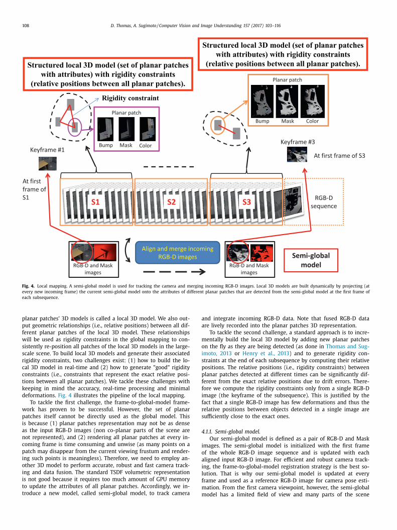
Fig. 4. Local mapping. A semi-global model is used for tracking the camera and merging incoming RGB-D images. Local 3D models are built dynamically by projecting (at

every new incoming frame) the current semi-global model onto the attributes of different planar patches that are detected from the semi-global model at the first frame of

each subsequence.

a

a

m

o

i

s

p

p

f

f

i

f

r

s

4

i

o

a

i

l

f

m

planar patches’ 3D models is called a local 3D model. We also out-

put geometric relationships (i.e., relative positions) between all dif-

ferent planar patches of the local 3D model. These relationships

will be used as rigidity constraints in the global mapping to con-

sistently re-position all patches of the local 3D models in the large-

scale scene. To build local 3D models and generate their associated

rigidity constraints, two challenges exist: (1) how to build the lo-

cal 3D model in real-time and (2) how to generate ”good” rigidity

constraints (i.e., constraints that represent the exact relative posi-

tions between all planar patches). We tackle these challenges with

keeping in mind the accuracy, real-time processing and minimal

deformations. Fig. 4 illustrates the pipeline of the local mapping.

To tackle the first challenge, the frame-to-global-model frame-

work has proven to be successful. However, the set of planar

patches itself cannot be directly used as the global model. This

is because (1) planar patches representation may not be as dense

as the input RGB-D images (non co-planar parts of the scene are

not represented), and (2) rendering all planar patches at every in-

coming frame is time consuming and unwise (as many points on a

patch may disappear from the current viewing frustum and render-

ing such points is meaningless). Therefore, we need to employ an-

other 3D model to perform accurate, robust and fast camera track-

ing and data fusion. The standard TSDF volumetric representation

is not good because it requires too much amount of GPU memory

to update the attributes of all planar patches. Accordingly, we in-

troduce a new model, called semi-global model, to track camera

m

nd integrate incoming RGB-D data. Note that fused RGB-D data

re lively recorded into the planar patches 3D representation.

To tackle the second challenge, a standard approach is to incre-

entally build the local 3D model by adding new planar patches

n the fly as they are being detected (as done in Thomas and Sug-

moto, 2013 or Henry et al., 2013 ) and to generate rigidity con-

traints at the end of each subsequence by computing their relative

ositions. The relative positions (i.e., rigidity constraints) between

lanar patches detected at different times can be significantly dif-

erent from the exact relative positions due to drift errors. There-

ore we compute the rigidity constraints only from a single RGB-D

mage (the keyframe of the subsequence). This is justified by the

act that a single RGB-D image has few deformations and thus the

elative positions between objects detected in a single image are

ufficiently close to the exact ones.

.1.1. Semi-global model.

Our semi-global model is defined as a pair of RGB-D and Mask

mages. The semi-global model is initialized with the first frame

f the whole RGB-D image sequence and is updated with each

ligned input RGB-D image. For efficient and robust camera track-

ng, the frame-to-global-model registration strategy is the best so-

ution. That is why our semi-global model is updated at every

rame and used as a reference RGB-D image for camera pose esti-

ation. From the first camera viewpoint, however, the semi-global

odel has a limited field of view and many parts of the scene

D. Thomas, A. Sugimoto / Computer Vision and Image Understanding 157 (2017) 103–116 109

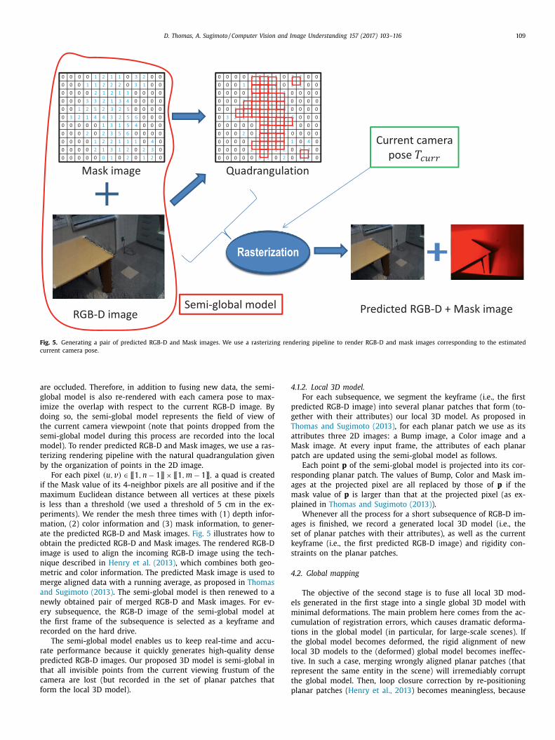
Fig. 5. Generating a pair of predicted RGB-D and Mask images. We use a rasterizing rendering pipeline to render RGB-D and mask images corresponding to the estimated

current camera pose.

a

g

i

d

t

s

m

t

b

i

m

i

p

m

a

o

i

n

m

m

a

n

e

t

r

r

p

t

c

f

4

p

g

T

a

M

p

r

a

m

p

a

s

k

s

4

e

m

c

t

t

l

t

r

t

p

re occluded. Therefore, in addition to fusing new data, the semi-

lobal model is also re-rendered with each camera pose to max-

mize the overlap with respect to the current RGB-D image. By

oing so, the semi-global model represents the field of view of

he current camera viewpoint (note that points dropped from the

emi-global model during this process are recorded into the local

odel). To render predicted RGB-D and Mask images, we use a ras-

erizing rendering pipeline with the natural quadrangulation given

y the organization of points in the 2D image.

For each pixel (u, v ) ∈ [[1 , n − 1]] × [[1 , m − 1]] , a quad is created

f the Mask value of its 4-neighbor pixels are all positive and if the

aximum Euclidean distance between all vertices at these pixels

s less than a threshold (we used a threshold of 5 cm in the ex-

eriments). We render the mesh three times with (1) depth infor-

ation, (2) color information and (3) mask information, to gener-

te the predicted RGB-D and Mask images. Fig. 5 illustrates how to

btain the predicted RGB-D and Mask images. The rendered RGB-D

mage is used to align the incoming RGB-D image using the tech-

ique described in Henry et al. (2013) , which combines both geo-

etric and color information. The predicted Mask image is used to

erge aligned data with a running average, as proposed in Thomas

nd Sugimoto (2013) . The semi-global model is then renewed to a

ewly obtained pair of merged RGB-D and Mask images. For ev-

ry subsequence, the RGB-D image of the semi-global model at

he first frame of the subsequence is selected as a keyframe and

ecorded on the hard drive.

The semi-global model enables us to keep real-time and accu-

ate performance because it quickly generates high-quality dense

redicted RGB-D images. Our proposed 3D model is semi-global in

hat all invisible points from the current viewing frustum of the

amera are lost (but recorded in the set of planar patches that

orm the local 3D model).

.1.2. Local 3D model.

For each subsequence, we segment the keyframe (i.e., the first

redicted RGB-D image) into several planar patches that form (to-

ether with their attributes) our local 3D model. As proposed in

homas and Sugimoto (2013) , for each planar patch we use as its

ttributes three 2D images: a Bump image, a Color image and a

ask image. At every input frame, the attributes of each planar

atch are updated using the semi-global model as follows.

Each point p of the semi-global model is projected into its cor-

esponding planar patch. The values of Bump, Color and Mask im-

ges at the projected pixel are all replaced by those of p if the

ask value of p is larger than that at the projected pixel (as ex-

lained in Thomas and Sugimoto (2013) ).

Whenever all the process for a short subsequence of RGB-D im-

ges is finished, we record a generated local 3D model (i.e., the

et of planar patches with their attributes), as well as the current

eyframe (i.e., the first predicted RGB-D image) and rigidity con-

traints on the planar patches.

.2. Global mapping

The objective of the second stage is to fuse all local 3D mod-

ls generated in the first stage into a single global 3D model with

inimal deformations. The main problem here comes from the ac-

umulation of registration errors, which causes dramatic deforma-

ions in the global model (in particular, for large-scale scenes). If

he global model becomes deformed, the rigid alignment of new

ocal 3D models to the (deformed) global model becomes ineffec-

ive. In such a case, merging wrongly aligned planar patches (that

epresent the same entity in the scene) will irremediably corrupt

he global model. Then, loop closure correction by re-positioning

lanar patches ( Henry et al., 2013 ) becomes meaningless, because

110 D. Thomas, A. Sugimoto / Computer Vision and Image Understanding 157 (2017) 103–116

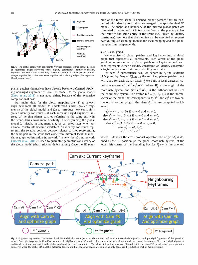
Fig. 6. The global graph with constraints. Vertices represent either planar patches

or keyframes. Edges represent either rigidity constraints, identity constraint,

keyframe pose constraints or visibility constraints. Note that similar patches are not

merged together but rather connected together with identity edges (that represent

identity constraints).

n

n

m

c

t

c

e

m

4

g

g

e

a

o

w

o

c

t

v

t

l

w

fi

l

planar patches themselves have already become deformed. Apply-

ing non-rigid alignment of local 3D models to the global model

( Zhou et al., 2013 ) is not good either, because of the expensive

computational cost.

Our main ideas for the global mapping are (1) to always

align new local 3D models to undeformed subsets (called frag-

ments) of the global model and (2) to introduce new constraints

(called identity constraints) at each successful rigid alignment, in-

stead of merging planar patches referring to the same entity in

the scene. This allows more flexibility in re-organizing the global

model (a mistake in alignment may be corrected later when ad-

ditional constraints become available). An identity constraint rep-

resents the relative position between planar patches representing

the same part in the scene that come from different local 3D mod-

els. A graph optimization framework (namely, the g2o framework

Cameral et al., 2011 ) is used to guarantee geometric consistency of

the global model (thus reducing deformations). Once the 3D scan-

Fig. 7. Fragment registration. The current local 3D model (that corresponds to the curre

model. One rigid fragment is identified as a set of neighboring local 3D models that c

additional constraints are added to the global graph and the graph is optimized. This allow

only, even when the global 3D model is deformed (due to multiple loops for example). E

ing of the target scene is finished, planar patches that are con-

ected with identity constraints are merged to output the final 3D

odel. The shape and boundary of the merged planar patch are

omputed using redundant information from all the planar patches

hat refer to the same entity in the scene (i.e., linked by identity

onstraints). We note that the merging can be executed on request

ven during 3D scanning because the local mapping and the global

apping run independently.

.2.1. Global graph.

We organize all planar patches and keyframes into a global

raph that represents all constraints. Each vertex of the global

raph represents either a planar patch or a keyframe, and each

dge represents either a rigidity constraint, an identity constraint,

keyframe pose constraint or a visibility constraint.

For each i th subsequence Seq i , we denote by K i the keyframe

f Seq i and by P set i = { P i j } j∈ [1: m i ]

the set of m i planar patches built

ith Seq i . For each planar patch P i j

we build a local Cartesian co-

rdinate system (�i j , e

i, j 1

, e i, j 2

, n

i, j ) , where �i j

is the origin of the

oordinate system and (e i, j 1

, e i, j 2

, n

i, j ) is the orthonormal basis of

he coordinate system. The vector n

i, j = (n x , n y , n z ) is the normal

ector of the plane that corresponds to P i j . e

i, j 1

and e i, j 2

are two or-

honormal vectors lying in the plane P i j

that are computed as fol-

ows:

e i, j 1

= (−n y , n x , 0) if n x � = 0 and n y � = 0 ,

else e i, j 1

= (−n z , 0 , n x ) if n x � = 0 and n z � = 0 ,

else e i, j 1

= (0 , −n z , n y ) if n y � = 0 and n z � = 0 ,

else e i, j 1

= (1 , 0 , 0) if n y � = 0 or n z � = 0 ,

else e i, j 1

= (0 , 1 , 0) .

e i, j 2

= n

i, j ∧ e i, j 1

,

here ∧ denotes the cross product operator. The origin �i j

is de-

ned as the 3D position (in the global coordinate system) of the

ower left corner of the bounding box for P i j

(with the oriented

nt keyframe) is successively aligned to multiple rigid fragments of the global 3D

orrespond to keyframes with successive timestamps. After each rigid alignment,

s integrating new local 3D models into the global 3D model using rigid registration

mploying only dense rigid registration enables fast processing.

D. Thomas, A. Sugimoto / Computer Vision and Image Understanding 157 (2017) 103–116 111

c

v

V

M

t

w

p

o

T

t

t

T

w

h

t

r

c

c

m

4

a

s

t

Fig. 8. Efficient registration of the current local 3D model using GICP with projec-

tive data association. For each point in the current local 3D model, its correspond-

ing point (i.e., approximated closest point) in the global 3D model is estimated in

a few comparisons by projecting it into the different planar patches that compose

the reference rigid fragment (which corresponds to the local 3D model of a single

keyframe (the previous one) in this simple example). Closest point association is

run efficiently on the GPU for fast GICP alignment.

P

n

s

i

t

i

a

w

s

F

g

S

w

t

i

k

{

.

m

a

m

c

W

k

r

s

i

c

u

F

f

t

t

t

e

oordinate system). Each planar patch P i j

is then represented as a

ertex in the graph to which the matrix of basis V i j

is assigned:

i j =

[e i, j

1 e i, j

2 n

i, j �i j

0 0 0 1

].

atrix V i j

transforms 3D points from the world coordinate system

o the local coordinate system of P i j .

Each keyframe K i is represented as a vertex in the graph to

hich its pose (4 × 4 matrix) T i (computed during the local map-

ing) is assigned. Note that V i j

and T i are the variables in our graph

ptimization problem. Our objective is to find the optimal V i j

and

i with respect to the observations (i.e., the set of constraints).

To each edge e = (a, b) that connects two vertices a and b , with

ransformation matrices T a and T b (respectively), we assign a 3D

ransformation matrix T edge that defines the following constraint:

b T −1

a T −1 edge

= Id ,

here Id is the 4 × 4 identity matrix. We detail in the following

ow to compute T edge for each type of edges. In the remaining of

his paper, we will replace T edge by T Rig

i, j,k , T Id

i,k, j,l , T

Key i,i +1

or T Vis i, j

when

eferring to rigidity constraints, identity constraints, keyframe pose

onstraints or visibility constraints (respectively). Note that once

reated, the value of each edge remains fixed during the global

apping (while the values of T a and T b are optimized).

1. Rigidity constraints. For each subsequence Seq i we generate

edges that connect all planar patches with each other. For each

edge (P i j , P i

k ) we assign matrix T

Rig

i, j,k = V i

k (V i

j ) −1 (i.e., the relative

position) that defines the rigidity constraint between P i j

and P i k .

These edges are created at the end of each local mapping. Note

that P i j

and P i k

are built from the same subsequence Seq i .

2. Identity constraints. Identity constraints are defined by the rel-

ative positions between planar patches representing the same

part of the scene (by abuse we will say that the planar patches

are identical). Every time a set of patches Pset i is registered to

another set of patches Pset j , we generate edges that represent

identity constraints. We first identify identical planar patches as

follows. Two planar patches P i k

and P j

l are identical if and only

if ‖ d i,k − d j,l ‖ < τ1 , n

i, k · n

j, l > τ 2 and overlap (P i k , P

j

l ) > τ3 ,

where · is the scalar product, overlap (P i k , P

j

l ) is a function that

counts the number of overlapping pixels between P i k

and P j

l and

τ 1 , τ 2 and τ 3 are three thresholds (e.g.10cm, 20 ° and 30 0 0

points respectively in the experiments). For every pair of iden-

tical planar patches (P i k , P

j

l ) we generate an edge, and assign to

it matrix T Id i,k, j,l

= V j

l (V i

k ) −1 that defines the identity constraint.

Note that i � = j .

3. Keyframe pose constraints ( Henry et al., 2013 ). For every two

successive subsequences Seq i and Seq i +1 , we generate an edge

(K i , K i +1 ) , and assign to it matrix T Key

i,i +1 = T i +1 T

−1 i

that defines

the keyframe pose constraint between K i and K i +1 .

4. Visibility constraints ( Henry et al., 2013 ). For each subse-

quence Seq i we generate edges so that K i is connected with any

planar patch in Pset i . To each edge (K i , P i j ) , we assign to it ma-

trix T Vis i, j

= V i j T −1

i that defines the visibility constraint between

P i j

and K i .

.2.2. On-line fragment registration with update of global graph.

The global graph grows every time a local 3D model is gener-

ted. Once a local model Pset i comes, we first add vertices corre-

ponding to each planar patch P i j

and a vertex corresponding to

he keyframe K . We then add edges so that all planar patches in

i

set i are connected with each other, K i and K i −1 (if i > 1) are con-

ected, and K i and any entry in Pset i are connected (they repre-

ent the rigidity constraints, keyframe pose constraint and visibil-

ty constraints respectively).

Second, we perform the fragment registration of Pset i with mul-

iple fragments (i.e., undeformed subsets) of the global graph to

nclude Pset i into the global model while minimizing deformations

s much as possible. We first identify a set of keyframes each of

hich is sufficiently close to K i , and divide the set into fragments

o that each fragment consists of only successive keyframes (see

ig. 7 ).

We define the set S i of the neighboring keyframes of K i in the

lobal graph as follows:

i = { K j | d(K i , K j ) < τd and α(K i , K j ) < τα} , here d ( K i , K j ) and α( K i , K j ) are the Euclidean distance between

he centres of two cameras, and the angle between the two view-

ng directions of the two cameras (respectively) for the i th and j th

eyframes (in the experiments, we set τd = 3 m and τα = 45 ◦).

We then break the set S i into p fragments: S i = F 1

i , F 2

i , . . . , F

p i } = {{ K s 1 , K s 1 +1 , K s 1 +2 , . . . , K s 1 + t 1 } , { K s 2 , K s 2 +1 , K s 2 +2 ,

. . , K s 2 + t 2 } , . . . , { K s p , K s p +1 , K s p +2 , . . . , K s p + t p }} where for all

j ∈ [1 : p − 1] , s j+1 > s j + t j + 1 . We reason that the local 3D

odels corresponding to successive keyframes that are close to K i

re registered together in a sufficiently correct (i.e., undeformed)

anner to perform rigid alignment with Pset i . This is not the

ase if the set of keyframes contains non-successive keyframes.

e denote by P set j i

the set of all planar patches connected to a

eyframe in F j

i ( j ∈ [1: p ]).

Next, we align Pset i with each of { P set j i } j∈ [1: p] . The (fragment)

egistration process of Pset i with a fragment P set j i

( j ∈ [1: p ]) con-

ists of an initialization step using sparse visual features detected

n each keyframe followed by the dense GICP. We detail this pro-

edure below.

The transformation that aligns Pset i with P set j i

is initialied by

sing matches of SIFT features ( Lowe, 1999 ) between K i and K s j (∈

j i ) . We use the RANSAC strategy here to have a set of matched

eatures. If the number of matched features is greater than a

hreshold (we used a threshold of 30 in our experiments), then

he transformation is initialized by the matched features; it is set

o the identity transformation otherwise.

After the initialization, we apply the GICP algorithm ( Segal

t al., 2009 ) to accurately align Pset i and P set j i . Because of millions

112 D. Thomas, A. Sugimoto / Computer Vision and Image Understanding 157 (2017) 103–116

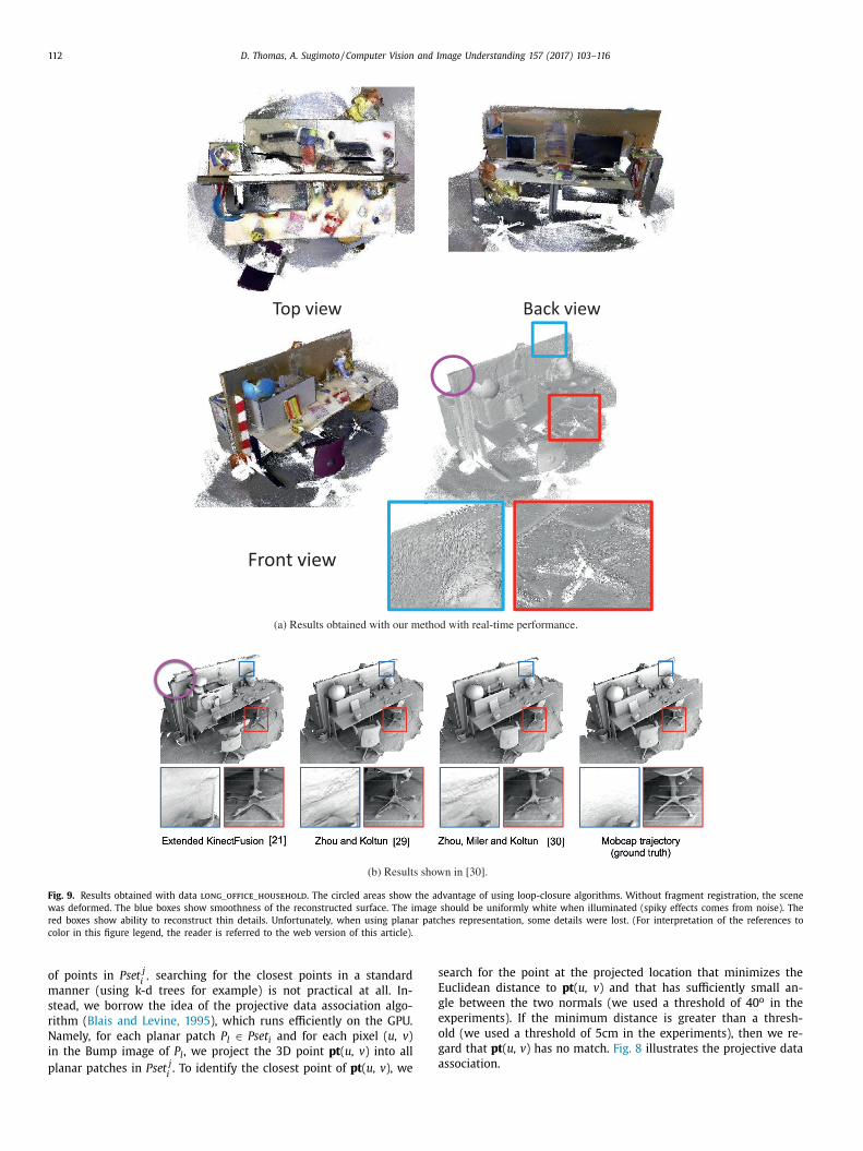
Fig. 9. Results obtained with data long_office_household . The circled areas show the advantage of using loop-closure algorithms. Without fragment registration, the scene

was deformed. The blue boxes show smoothness of the reconstructed surface. The image should be uniformly white when illuminated (spiky effects comes from noise). The

red boxes show ability to reconstruct thin details. Unfortunately, when using planar patches representation, some details were lost. (For interpretation of the references to

color in this figure legend, the reader is referred to the web version of this article).

s

E

g

e

o

g

association.

of points in P set j i , searching for the closest points in a standard

manner (using k-d trees for example) is not practical at all. In-

stead, we borrow the idea of the projective data association algo-

rithm ( Blais and Levine, 1995 ), which runs efficiently on the GPU.

Namely, for each planar patch P l ∈ Pset i and for each pixel ( u, v )

in the Bump image of P l , we project the 3D point pt ( u, v ) into all

planar patches in P set j i . To identify the closest point of pt ( u, v ), we

earch for the point at the projected location that minimizes the

uclidean distance to pt ( u, v ) and that has sufficiently small an-

le between the two normals (we used a threshold of 40 o in the

xperiments). If the minimum distance is greater than a thresh-

ld (we used a threshold of 5cm in the experiments), then we re-

ard that pt ( u, v ) has no match. Fig. 8 illustrates the projective data

D. Thomas, A. Sugimoto / Computer Vision and Image Understanding 157 (2017) 103–116 113

t

g

t

a

t

t

s

a

s

t

d

r

p

f

p

5

r

s

L

c

c

X

G

a

F

m

i

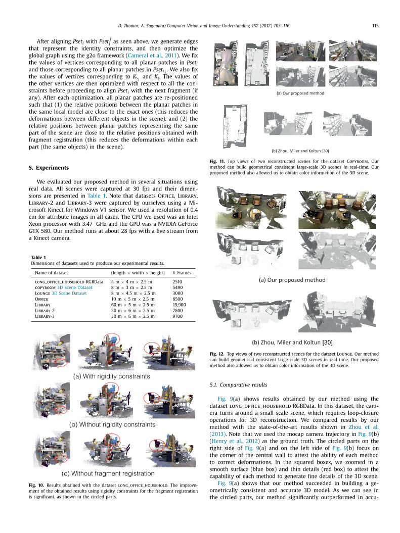
Fig. 11. Top views of two reconstructed scenes for the dataset Copyroom . Our

method can build geometrical consistent large-scale 3D scenes in real-time. Our

proposed method also allowed us to obtain color information of the 3D scene.

After aligning Pset i with P set j i

as seen above, we generate edges

hat represent the identity constraints, and then optimize the

lobal graph using the g2o framework ( Cameral et al., 2011 ). We fix

he values of vertices corresponding to all planar patches in Pset i nd those corresponding to all planar patches in P set s j . We also fix

he values of vertices corresponding to K s j and K i . The values of

he other vertices are then optimized with respect to all the con-

traints before proceeding to align Pset i with the next fragment (if

ny). After each optimization, all planar patches are re-positioned

uch that (1) the relative positions between the planar patches in

he same local model are close to the exact ones (this reduces the

eformations between different objects in the scene), and (2) the

elative positions between planar patches representing the same

art of the scene are close to the relative positions obtained with

ragment registration (this reduces the deformations within each

art (the same objects) in the scene).

. Experiments

We evaluated our proposed method in several situations using

eal data. All scenes were captured at 30 fps and their dimen-

ions are presented in Table 1 . Note that datasets Office , Library ,

ibrary-2 and Library-3 were captured by ourselves using a Mi-

rosoft Kinect for Windows V1 sensor. We used a resolution of 0.4

m for attribute images in all cases. The CPU we used was an Intel

eon processor with 3.47 GHz and the GPU was a NVIDIA GeForce

TX 580. Our method runs at about 28 fps with a live stream from

Kinect camera.

Table 1

Dimensions of datasets used to produce our experimental results.

Name of dataset (length × width × height) # Frames

long_office_household RGBData 4 m × 4 m × 2.5 m 2510

copyroom 3D Scene Dataset 8 m × 3 m × 2.5 m 5490

Lounge 3D Scene Dataset 8 m × 4.5 m × 2.5 m 30 0 0

Office 10 m × 5 m × 2.5 m 8500

Library 60 m × 5 m × 2.5 m 19 ,900

Library-2 20 m × 6 m × 2.5 m 7800

Library-3 30 m × 6 m × 2.5 m 9700

ig. 10. Results obtained with the dataset long_office_household . The improve-

ent of the obtained results using rigidity constraints for the fragment registration

s significant, as shown in the circled parts.

Fig. 12. Top views of two reconstructed scenes for the dataset Lounge . Our method

can build geometrical consistent large-scale 3D scenes in real-time. Our proposed

method also allowed us to obtain color information of the 3D scene.

5

d

e

o

m

(

(

r

t

t

s

c

o

t

.1. Comparative results

Fig. 9 (a) shows results obtained by our method using the

ataset long_office_household RGBData. In this dataset, the cam-

ra turns around a small scale scene, which requires loop-closure

perations for 3D reconstruction. We compared results by our

ethod with the state-of-the-art results shown in Zhou et al.

2013) . Note that we used the mocap camera trajectory in Fig. 9 (b)

Henry et al., 2012 ) as the ground truth. The circled parts on the

ight side of Fig. 9 (a) and on the left side of Fig. 9 (b) focus on

he corner of the central wall to attest the ability of each method

o correct deformations. In the squared boxes, we zoomed in a

mooth surface (blue box) and thin details (red box) to attest the

apability of each method to generate fine details of the 3D scene.

Fig. 9 (a) shows that our method succeeded in building a ge-

metrically consistent and accurate 3D model. As we can see in

he circled parts, our method significantly outperformed in accu-

114 D. Thomas, A. Sugimoto / Computer Vision and Image Understanding 157 (2017) 103–116

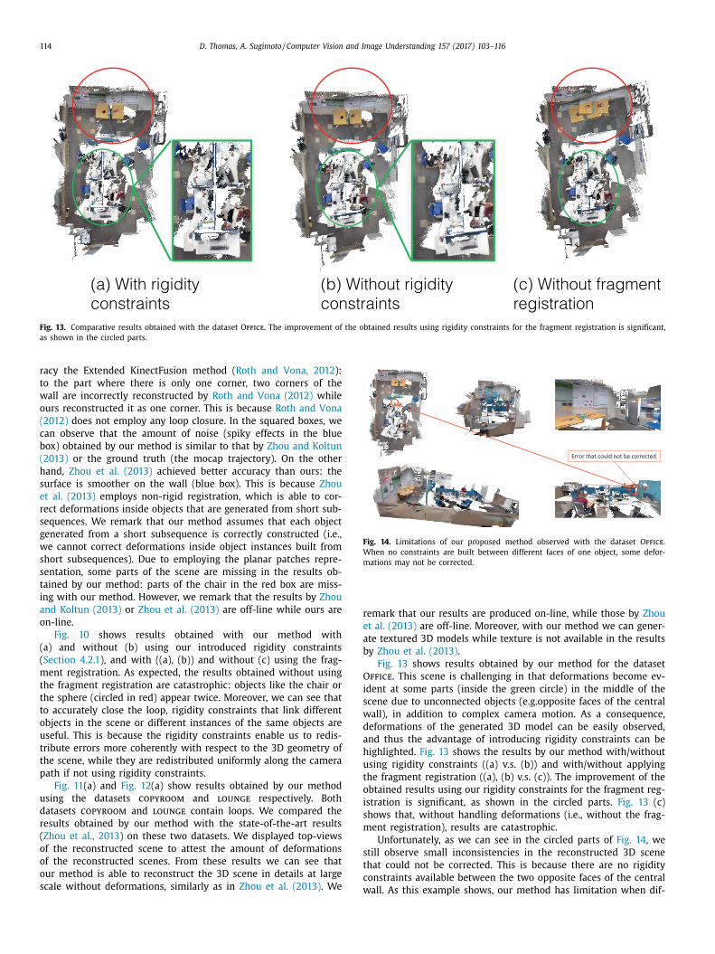
Fig. 13. Comparative results obtained with the dataset Office . The improvement of the obtained results using rigidity constraints for the fragment registration is significant,

as shown in the circled parts.

Fig. 14. Limitations of our proposed method observed with the dataset Office .

When no constraints are built between different faces of one object, some defor-

mations may not be corrected.

r

e

a

b

O

i

s

w

d

a

h

u

t

o

i

s

m

s

t

c

racy the Extended KinectFusion method ( Roth and Vona, 2012 ):

to the part where there is only one corner, two corners of the

wall are incorrectly reconstructed by Roth and Vona (2012) while

ours reconstructed it as one corner. This is because Roth and Vona

(2012) does not employ any loop closure. In the squared boxes, we

can observe that the amount of noise (spiky effects in the blue

box) obtained by our method is similar to that by Zhou and Koltun

(2013) or the ground truth (the mocap trajectory). On the other

hand, Zhou et al. (2013) achieved better accuracy than ours: the

surface is smoother on the wall (blue box). This is because Zhou

et al. (2013) employs non-rigid registration, which is able to cor-

rect deformations inside objects that are generated from short sub-

sequences. We remark that our method assumes that each object

generated from a short subsequence is correctly constructed (i.e.,

we cannot correct deformations inside object instances built from

short subsequences). Due to employing the planar patches repre-

sentation, some parts of the scene are missing in the results ob-

tained by our method: parts of the chair in the red box are miss-

ing with our method. However, we remark that the results by Zhou

and Koltun (2013) or Zhou et al. (2013) are off-line while ours are

on-line.

Fig. 10 shows results obtained with our method with

(a) and without (b) using our introduced rigidity constraints

( Section 4.2.1 ), and with ((a), (b)) and without (c) using the frag-

ment registration. As expected, the results obtained without using

the fragment registration are catastrophic: objects like the chair or

the sphere (circled in red) appear twice. Moreover, we can see that

to accurately close the loop, rigidity constraints that link different

objects in the scene or different instances of the same objects are

useful. This is because the rigidity constraints enable us to redis-

tribute errors more coherently with respect to the 3D geometry of

the scene, while they are redistributed uniformly along the camera

path if not using rigidity constraints.

Fig. 11 (a) and Fig. 12 (a) show results obtained by our method

using the datasets copyroom and lounge respectively. Both

datasets copyroom and lounge contain loops. We compared the

results obtained by our method with the state-of-the-art results

( Zhou et al., 2013 ) on these two datasets. We displayed top-views

of the reconstructed scene to attest the amount of deformations

of the reconstructed scenes. From these results we can see that

our method is able to reconstruct the 3D scene in details at large

scale without deformations, similarly as in Zhou et al. (2013) . We

w

emark that our results are produced on-line, while those by Zhou

t al. (2013) are off-line. Moreover, with our method we can gener-

te textured 3D models while texture is not available in the results

y Zhou et al. (2013) .

Fig. 13 shows results obtained by our method for the dataset

ffice . This scene is challenging in that deformations become ev-

dent at some parts (inside the green circle) in the middle of the

cene due to unconnected objects (e.g.opposite faces of the central

all), in addition to complex camera motion. As a consequence,

eformations of the generated 3D model can be easily observed,

nd thus the advantage of introducing rigidity constraints can be

ighlighted. Fig. 13 shows the results by our method with/without

sing rigidity constraints ((a) v.s. (b)) and with/without applying

he fragment registration ((a), (b) v.s. (c)). The improvement of the

btained results using our rigidity constraints for the fragment reg-

stration is significant, as shown in the circled parts. Fig. 13 (c)

hows that, without handling deformations (i.e., without the frag-

ent registration), results are catastrophic.

Unfortunately, as we can see in the circled parts of Fig. 14 , we

till observe small inconsistencies in the reconstructed 3D scene

hat could not be corrected. This is because there are no rigidity

onstraints available between the two opposite faces of the central

all. As this example shows, our method has limitation when dif-

D. Thomas, A. Sugimoto / Computer Vision and Image Understanding 157 (2017) 103–116 115

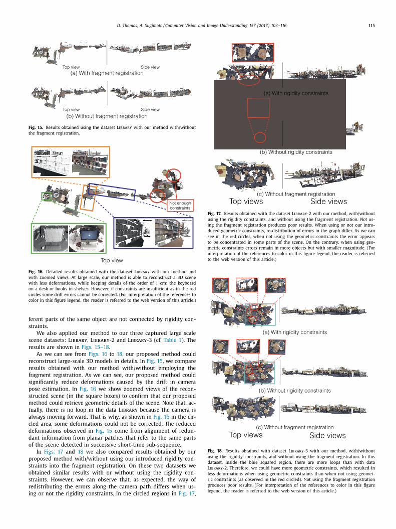
Fig. 15. Results obtained using the dataset Library with our method with/without

the fragment registration.

Fig. 16. Detailed results obtained with the dataset Library with our method and

with zoomed views. At large scale, our method is able to reconstruct a 3D scene

with less deformations, while keeping details of the order of 1 cm: the keyboard

on a desk or books in shelves. However, if constraints are insufficient as in the red

circles some drift errors cannot be corrected. (For interpretation of the references to

color in this figure legend, the reader is referred to the web version of this article.)

f

s

s

r

r

r

f

s

p

s

m

t

a

c

d

d

o

p

s

o

s

r

i

Fig. 17. Results obtained with the dataset Library-2 with our method, with/without

using the rigidity constraints, and without using the fragment registration. Not us-

ing the fragment registration produces poor results. When using or not our intro-

duced geometric constraints, re-distribution of errors in the graph differ. As we can

see in the red circles, when not using the geometric constraints the error appears

to be concentrated in some parts of the scene. On the contrary, when using geo-

metric constraints errors remain in more objects but with smaller magnitude. (For

interpretation of the references to color in this figure legend, the reader is referred

to the web version of this article.)

Fig. 18. Results obtained with dataset Library-3 with our method, with/without

using the rigidity constraints, and without using the fragment registration. In this

dataset, inside the blue squared region, there are more loops than with data

Library-2 . Therefore, we could have more geometric constraints, which resulted in

less deformations when using geometric constraints than when not using geomet-

ric constraints (as observed in the red circled). Not using the fragment registration

produces poor results. (For interpretation of the references to color in this figure

legend, the reader is referred to the web version of this article.)

erent parts of the same object are not connected by rigidity con-

traints.

We also applied our method to our three captured large scale

cene datasets: Library , Library-2 and Library-3 (cf. Table 1 ). The

esults are shown in Figs. 15–18 .

As we can see from Figs. 16 to 18 , our proposed method could

econstruct large-scale 3D models in details. In Fig. 15 , we compare

esults obtained with our method with/without employing the

ragment registration. As we can see, our proposed method could

ignificantly reduce deformations caused by the drift in camera

ose estimation. In Fig. 16 we show zoomed views of the recon-

tructed scene (in the square boxes) to confirm that our proposed

ethod could retrieve geometric details of the scene. Note that, ac-

ually, there is no loop in the data Library because the camera is

lways moving forward. That is why, as shown in Fig. 16 in the cir-

led area, some deformations could not be corrected. The reduced

eformations observed in Fig. 15 come from alignment of redun-

ant information from planar patches that refer to the same parts

f the scene detected in successive short-time sub-sequence.

In Figs. 17 and 18 we also compared results obtained by our

roposed method with/without using our introduced rigidity con-

traints into the fragment registration. On these two datasets we

btained similar results with or without using the rigidity con-

traints. However, we can observe that, as expected, the way of

edistributing the errors along the camera path differs when us-

ng or not the rigidity constraints. In the circled regions in Fig. 17 ,

116 D. Thomas, A. Sugimoto / Computer Vision and Image Understanding 157 (2017) 103–116

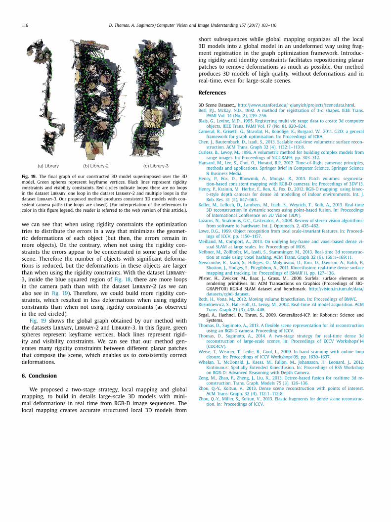
Fig. 19. The final graph of our constructed 3D model superimposed over the 3D

model. Green spheres represent keyframe vertices. Black lines represent rigidity

constraints and visibility constraints. Red circles indicate loops: there are no loops

in the dataset Library , one loop in the dataset Library-2 and multiple loops in the

dataset Library-3 . Our proposed method produces consistent 3D models with con-

sistent camera paths (the loops are closed). (For interpretation of the references to

color in this figure legend, the reader is referred to the web version of this article.).

s

3

m

i

p

p

r

R

3

B

B

C

C

C

H

H

H

K

L

L

N

N

P

R

S

T

T

W

W

Z

Z

Z

we can see that when using rigidity constraints the optimization

tries to distribute the errors in a way that minimizes the geomet-

ric deformations of each object (but then, the errors remain in

more objects). On the contrary, when not using the rigidity con-

straints the errors appear to be concentrated in some parts of the

scene. Therefore the number of objects with significant deforma-

tions is reduced, but the deformations in these objects are larger

than when using the rigidity constraints. With the dataset Library-

3 , inside the blue squared region of Fig. 18 , there are more loops

in the camera path than with the dataset Library-2 (as we can

also see in Fig. 19 ). Therefore, we could build more rigidity con-

straints, which resulted in less deformations when using rigidity

constraints than when not using rigidity constraints (as observed

in the red circled).

Fig. 19 shows the global graph obtained by our method with

the datasets Library , Library-2 and Library-3 . In this figure, green

spheres represent keyframe vertices, black lines represent rigid-

ity and visibility constraints. We can see that our method gen-

erates many rigidity constraints between different planar patches

that compose the scene, which enables us to consistently correct

deformations.

6. Conclusion

We proposed a two-stage strategy, local mapping and global

mapping, to build in details large-scale 3D models with mini-

mal deformations in real time from RGB-D image sequences. The

local mapping creates accurate structured local 3D models from

hort subsequences while global mapping organizes all the local

D models into a global model in an undeformed way using frag-

ent registration in the graph optimization framework. Introduc-

ng rigidity and identity constraints facilitates repositioning planar

atches to remove deformations as much as possible. Our method

roduces 3D models of high quality, without deformations and in

eal-time, even for large-scale scenes.

eferences

D Scene Dataset:,. http://www.stanford.edu/ ∼qianyizh/projects/scenedata.html .

esl, P.J. , McKay, N.D. , 1992. A method for registration of 3-d shapes. IEEE Trans.PAMI Vol. 14 (No. 2), 239–256 .

lais, G. , Levine, M.D. , 1995. Registering multi vie range data to create 3d computerobjects. IEEE Trans. PAMI Vol. 17 (No. 8), 820–824 .

ameral, R. , Grisetti, G. , Strasdat, H. , Konolige, K. , Burgard, W. , 2011. G2O: a general

framework for graph optimisation. In: Proceedings of ICRA . hen, J. , Bautembach, D. , Izadi, S. , 2013. Scalable real-time volumetric surface recon-

struction. ACM Trans. Graph 32 (4), 1132:1–113:8 . urless, B. , Levoy, M. , 1996. A volumetric method for building complex models from

range images. In: Proceedings of SIGGRAPH, pp. 303–312 . ansard, M. , Lee, S. , Choi, O. , Horaud, R.P. , 2012. Time-of-flight cameras: principles,

methods and applications. Springer Brief in Computer Science. Springer Science

& Business Media . enry, P. , Fox, D. , Bhowmik, A. , Mongia, R. , 2013. Patch volumes: segmenta-

tion-based consistent mapping with RGB-D cameras. In: Proceedings of 3DV’13 .enry, P. , Krainin, M. , Herbst, E. , Ren, X. , Fox, D. , 2012. RGB-D mapping: using kinec-

t-style depth cameras for dense 3d modelling of indoor environments. Int. J.Rob. Res. 31 (5), 647–663 .

eller, M. , Lefloch, D. , Lambers, M. , Izadi, S. , Weyrich, T. , Kolb, A. , 2013. Real-time3D reconstruction in dynamic scenes using point-based fusion. In: Proceedings

of International Conference on 3D Vision (3DV) .

azaros, N. , Sirakoulis, G.C. , Gasteratos, A. , 2008. Review of stereo vision algorithms:from software to hardware. Int. J. Optomech. 2, 435–462 .

owe, D.G. , 1999. Object recognition from local scale-invariant features. In: Proceed-ings of ICCV, pp. 1150–1157 .

Meilland, M. , Comport, A. , 2013. On unifying key-frame and voxel-based dense vi-sual SLAM at large scales. In: Proceedings of IROS .

eibner, M. , Zollhofer, M. , Izadi, S. , Stamminger, M. , 2013. Real-time 3d reconstruc-

tion at scale using voxel hashing. ACM Trans. Graph 32 (6), 169:1–169:11 . ewcombe, R. , Izadi, S. , Hilliges, O. , Molyneaux, D. , Kim, D. , Davison, A. , Kohli, P. ,

Shotton, J. , Hodges, S. , Fitzgibbon, A. , 2011. Kinectfusion: real-time dense surfacemapping and tracking. In: Proceedings of ISMAR’11, pp. 127–136 .

fister, H., Zwicker, M., Baar, J., Gross, M., 20 0 0. Surfels: surface elements asrendering primitives. In: ACM Transactions on Graphics (Proceedings of SIG-

GRAPH’00) RGB-d SLAM dataset and benchmark . http://vision.in.tum.de/data/

datasets/rgbd-dataset . oth, H. , Vona, M. , 2012. Moving volume kinectfusion. In: Proceedings of BMVC .

Rusinkiewicz, S. , Hall-Holt, O. , Levoy, M. , 2002. Real-time 3d model acquisition. ACMTrans. Graph 21 (3), 438–446 .

egal, A., Haehnel, D., Thrun, S., 2009. Generalized-ICP. In: Robotics: Science andSystems.

homas, D. , Sugimoto, A. , 2013. A flexible scene representation for 3d reconstruction

using an RGB-D camera. Proceeding of ICCV . homas, D. , Sugimoto, A. , 2014. A two-stage strategy for real-time dense 3d

reconstruction of large-scale scenes. In: Proceedings of ECCV Workshops’14(CDC4CV) .

eise, T. , Wismer, T. , Leibe, B. , Gool, L. , 2009. In-hand scanning with online loopclosure. In: Proceedings of ICCV Workshops’09, pp. 1630–1637 .

helan, T. , McDonald, J. , Kaess, M. , Fallon, M. , Johansson, H. , Leonard, J. , 2012.

Kintinuous: Spatially Extended Kinectfusion. In: Proceedings of RSS Workshopon RGB-D: Advanced Reasoning with Depth Camera .

eng, M. , Zhao, F. , Zheng, J. , Liu, X. , 2013. Octree-based fusion for realtime 3d re-construction. Trans. Graph. Models 75 (3), 126–136 .

hou, Q.-Y. , Koltun, V. , 2013. Dense scene reconstruction with points of interest.ACM Trans. Graph. 32 (4), 112:1–112:8 .

hou, Q.-Y. , Miller, S. , Koltun, V. , 2013. Elastic fragments for dense scene reconstruc-

tion. In: Proceedings of ICCV .