Computer Vision and Computer Graphics: Two sides of a coin

COS 116: Apr 19, 2011

Sanjeev Arora

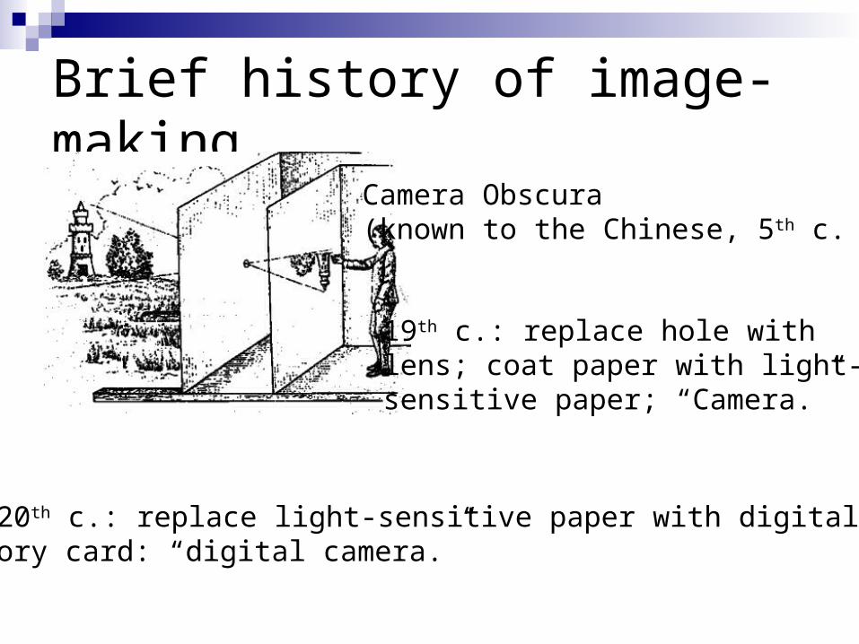
Brief history of image-making

Camera Obscura(known to the Chinese, 5th c. BC)

19th c.: replace hole with lens; coat paper with light-sensitive paper; “Camera.”

Late 20th c.: replace light-sensitive paper with digital sensor+ memory card: “digital camera.”

Theme 1: What is an image?

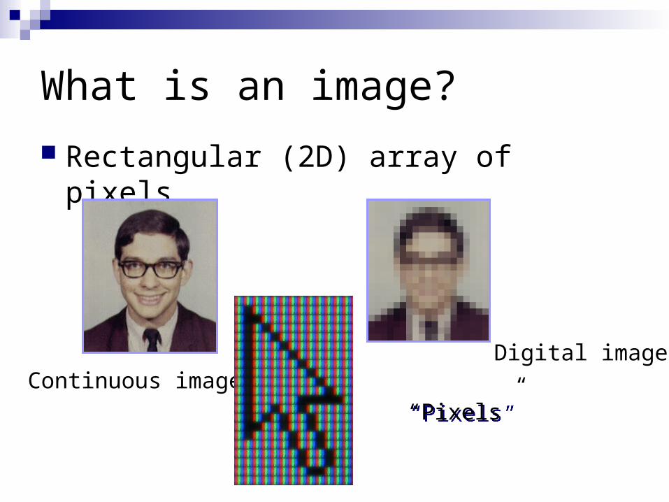
What is an image?

Rectangular (2D) array of pixels

Continuous imageDigital image

“Pixels”“Pixels”

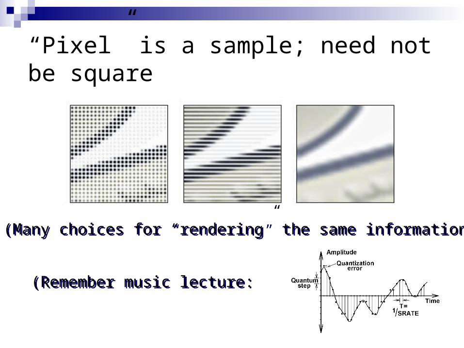
“Pixel” is a sample; need not be square

(Many choices for “rendering” the same information)(Many choices for “rendering” the same information)

(Remember music lecture: (Remember music lecture:

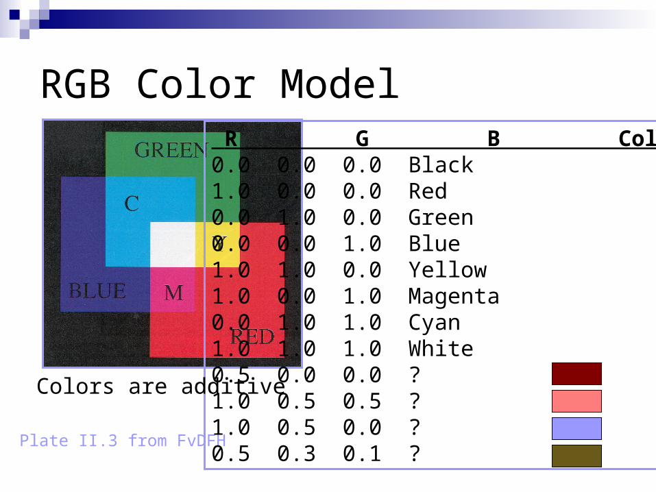
RGB Color Model

Plate II.3 from FvDFH

R G B Color 0.0 0.0 0.0 Black1.0 0.0 0.0 Red0.0 1.0 0.0 Green0.0 0.0 1.0 Blue1.0 1.0 0.0 Yellow1.0 0.0 1.0 Magenta0.0 1.0 1.0 Cyan1.0 1.0 1.0 White0.5 0.0 0.0 ?1.0 0.5 0.5 ?1.0 0.5 0.0 ?0.5 0.3 0.1 ?

Colors are additive

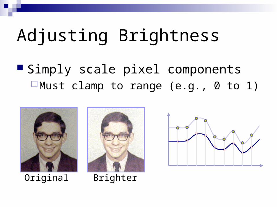
Adjusting Brightness

Simply scale pixel componentsMust clamp to range (e.g., 0 to 1)

Original Brighter

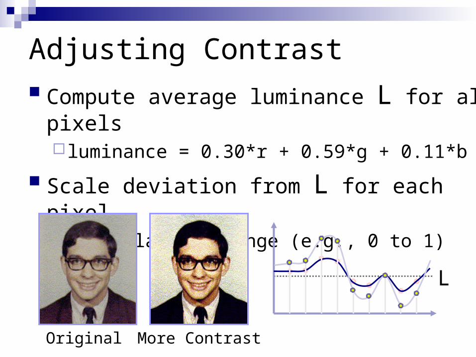
Adjusting Contrast Compute average luminance L for all pixels

luminance = 0.30*r + 0.59*g + 0.11*b

Scale deviation from L for each pixelMust clamp to range (e.g., 0 to 1)

Original More Contrast

L

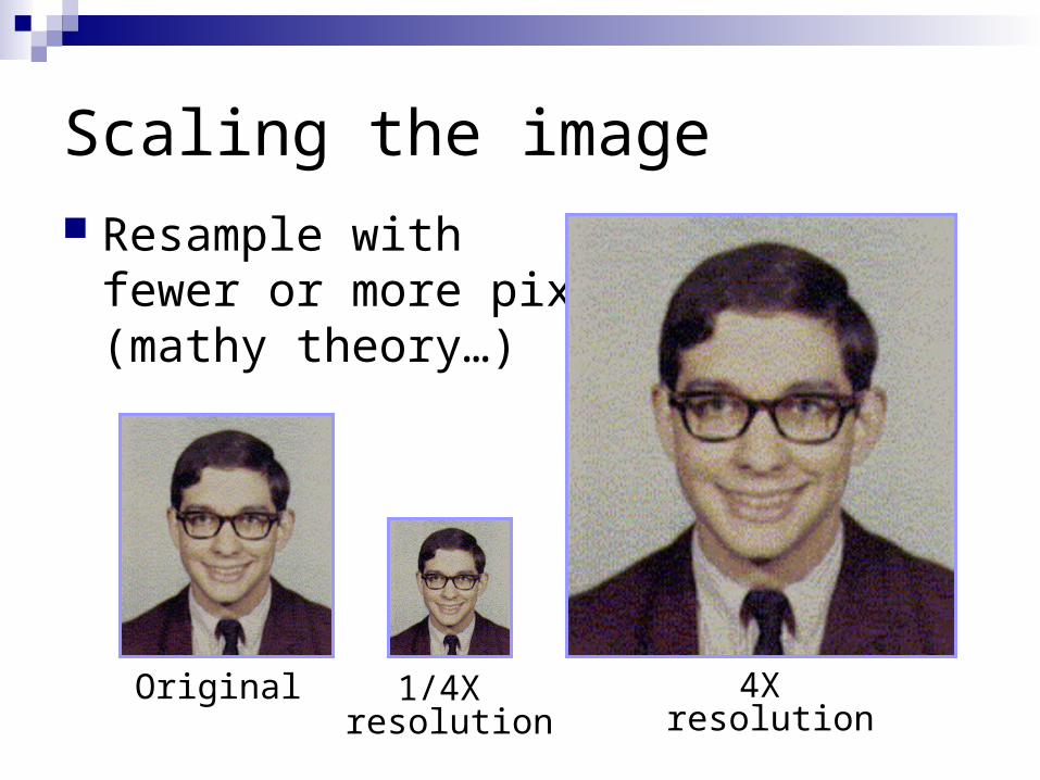
Scaling the image Resample with

fewer or more pixels(mathy theory…)

Original 1/4X resolution

4X resolution

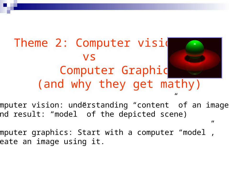
Theme 2: Computer vision vs

Computer Graphics (and why they get mathy)

Computer vision: understanding “content” of an image(end result: “model” of the depicted scene)

Computer graphics: Start with a computer “model”,create an image using it.

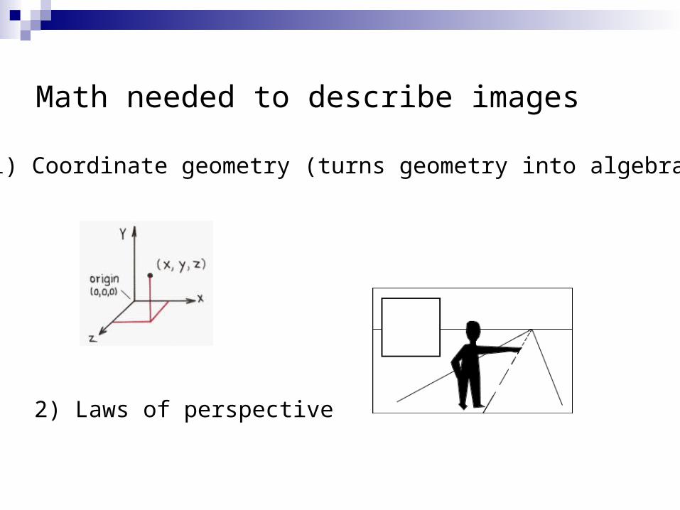
Math needed to describe images

(1) Coordinate geometry (turns geometry into algebra)

2) Laws of perspective

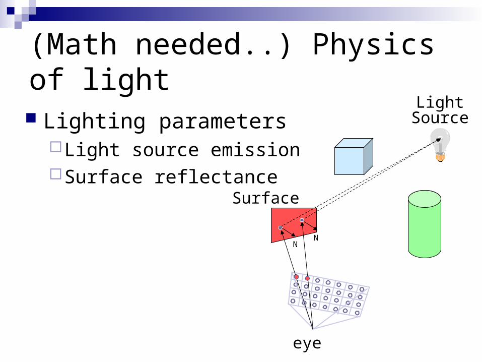
(Math needed..) Physics of light

Lighting parametersLight source emissionSurface reflectance

NN

eye

Surface

LightSource

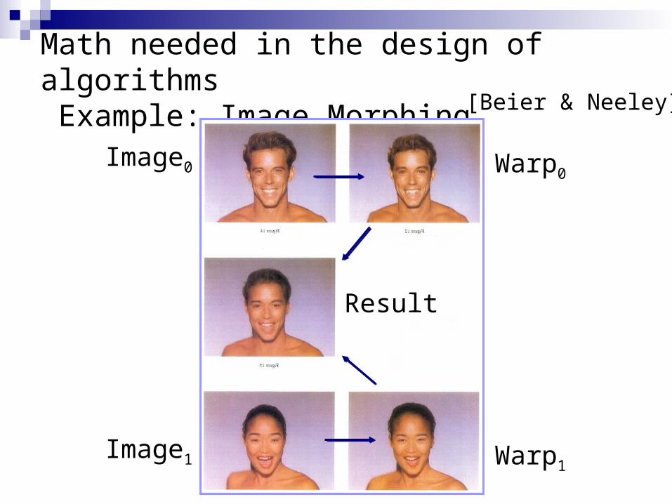
Math needed in the design of algorithms Example: Image Morphing

Image0

Image1

Warp0

Warp1

[Beier & Neeley]

Result

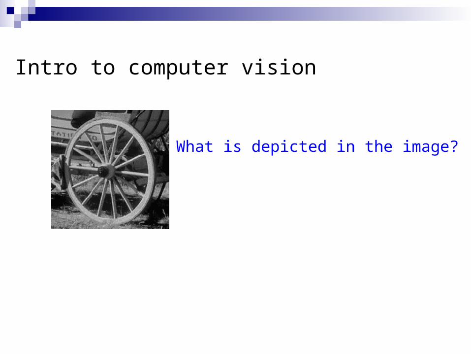
Intro to computer vision

What is depicted in the image?

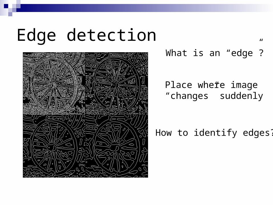
Edge detectionWhat is an “edge”?

Place where image“changes” suddenly

How to identify edges?

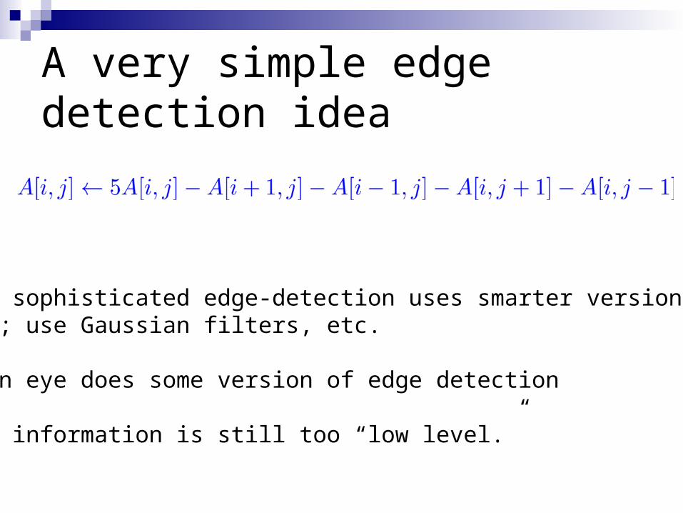
A very simple edge detection idea

More sophisticated edge-detection uses smarter versions ofthis; use Gaussian filters, etc.

Human eye does some version of edge detection

Edge information is still too “low level.”

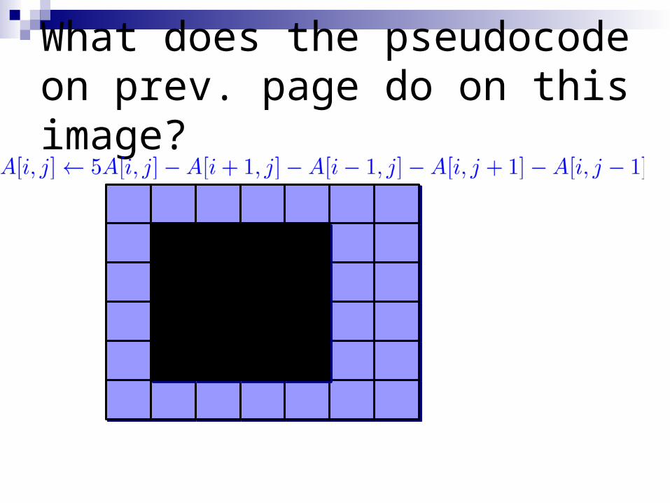
What does the pseudocode on prev. page do on this image?

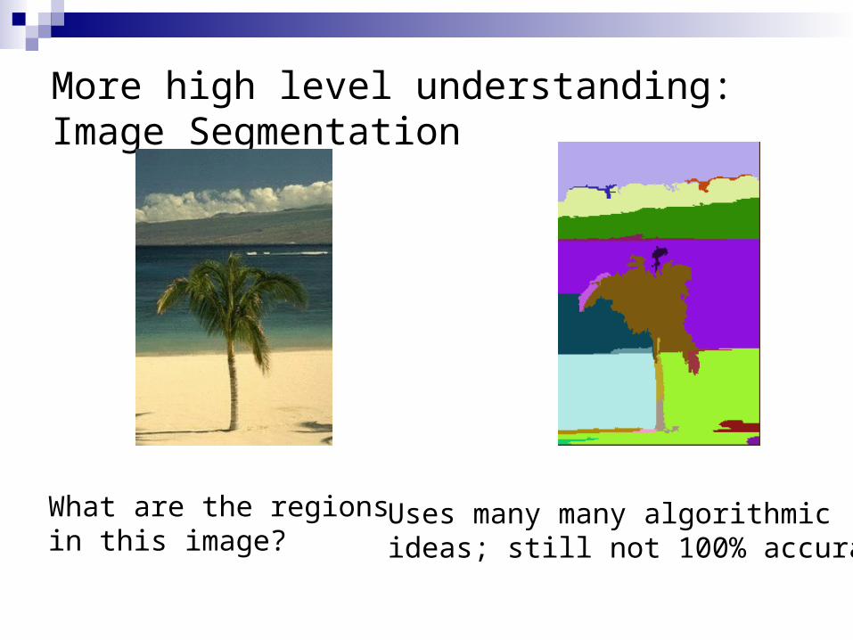
More high level understanding: Image Segmentation

What are the regions in this image?

Uses many many algorithmicideas; still not 100% accurate

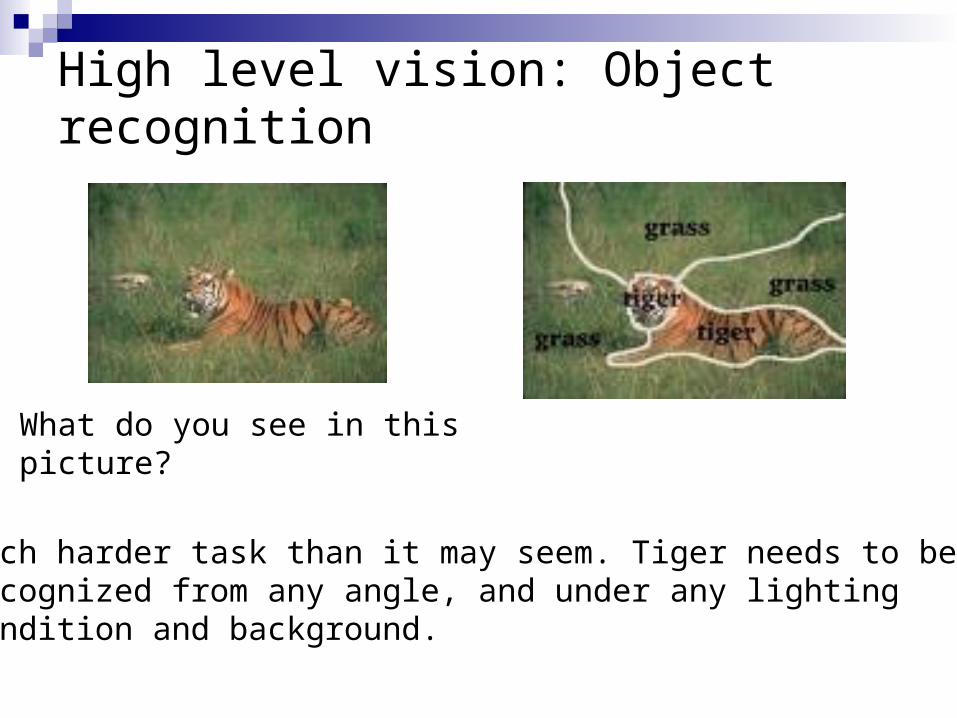
High level vision: Object recognition

Much harder task than it may seem. Tiger needs to berecognized from any angle, and under any lighting condition and background.

What do you see in this picture?

Aside

At least 8 “levels” in human vision system.Object recognition seems to require transfer ofinformation between levels, and the highest levels seem tied to restof intelligence.

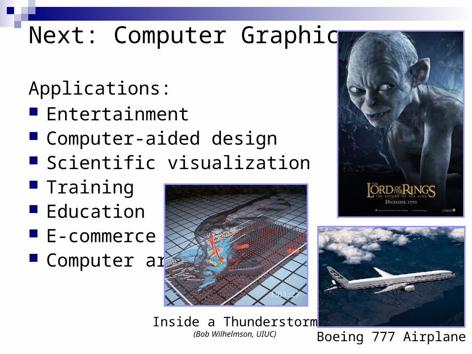
Next: Computer Graphics

Applications: Entertainment Computer-aided design Scientific visualization Training Education E-commerce Computer art

Boeing 777 AirplaneInside a Thunderstorm

(Bob Wilhelmson, UIUC)

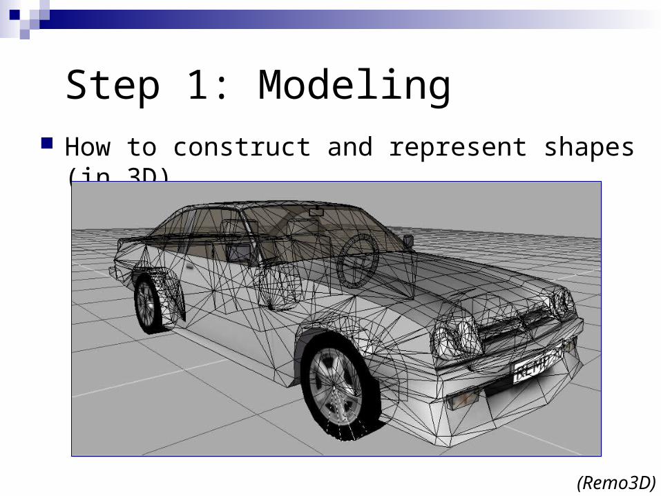
Step 1: Modeling How to construct and represent shapes (in 3D)

(Remo3D)

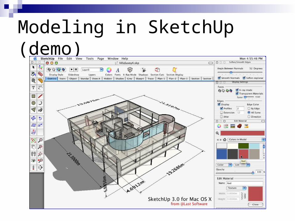
Modeling in SketchUp (demo)

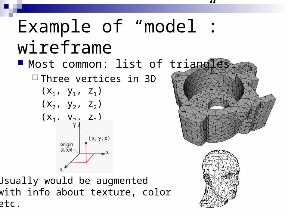
Example of “model”: wireframe Most common: list of triangles

Three vertices in 3D(x1, y1, z1)(x2, y2, z2)(x3, y3, z3)

Usually would be augmentedwith info about texture, coloretc.

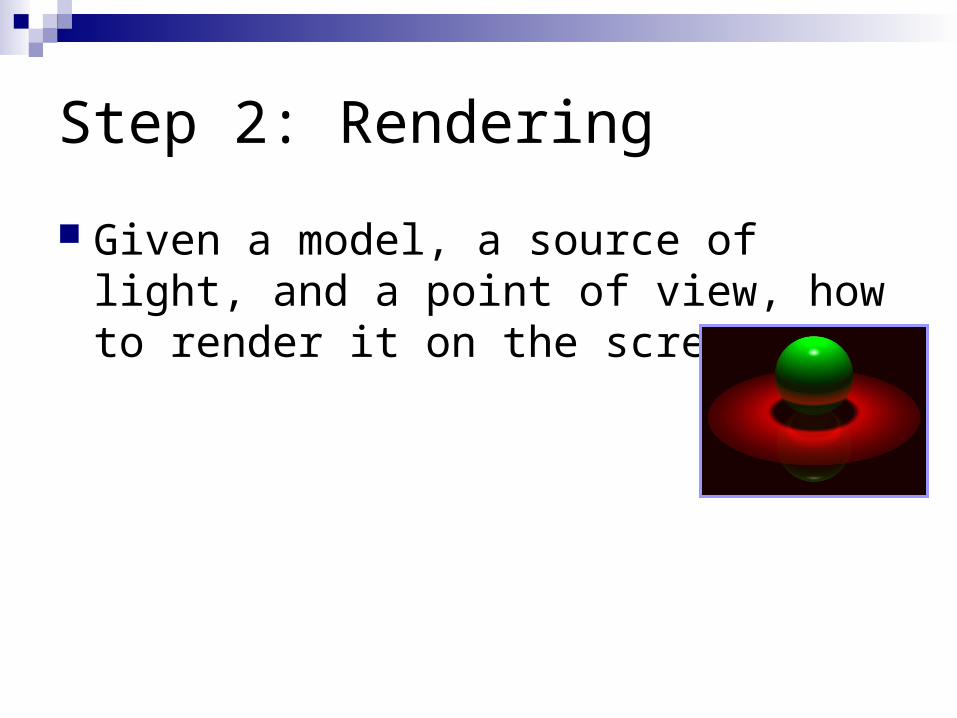
Step 2: Rendering

Given a model, a source of light, and a point of view, how to render it on the screen?

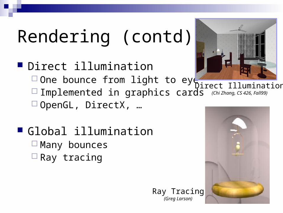
Rendering (contd)

Direct illumination One bounce from light to eye Implemented in graphics cards OpenGL, DirectX, …

Global illumination Many bounces Ray tracing

Direct Illumination(Chi Zhang, CS 426, Fall99)

Ray Tracing(Greg Larson)

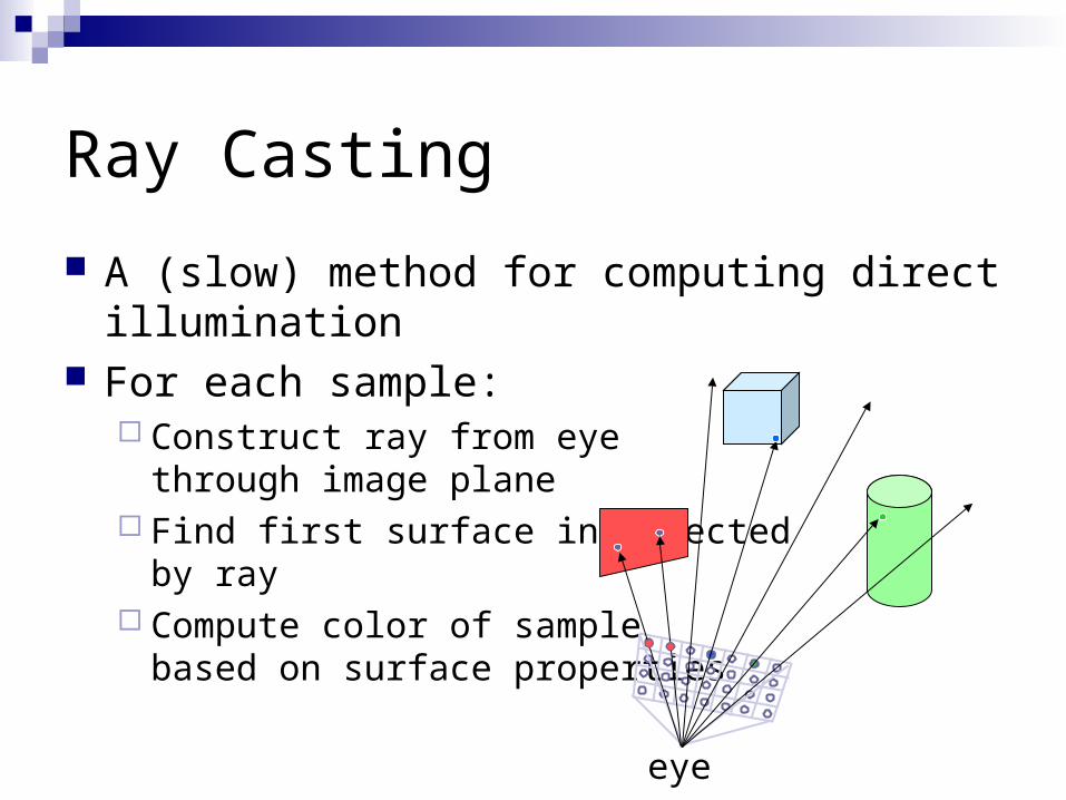
Ray Casting

A (slow) method for computing direct illumination For each sample:

Construct ray from eye through image plane

Find first surface intersectedby ray

Compute color of sample based on surface properties

eye

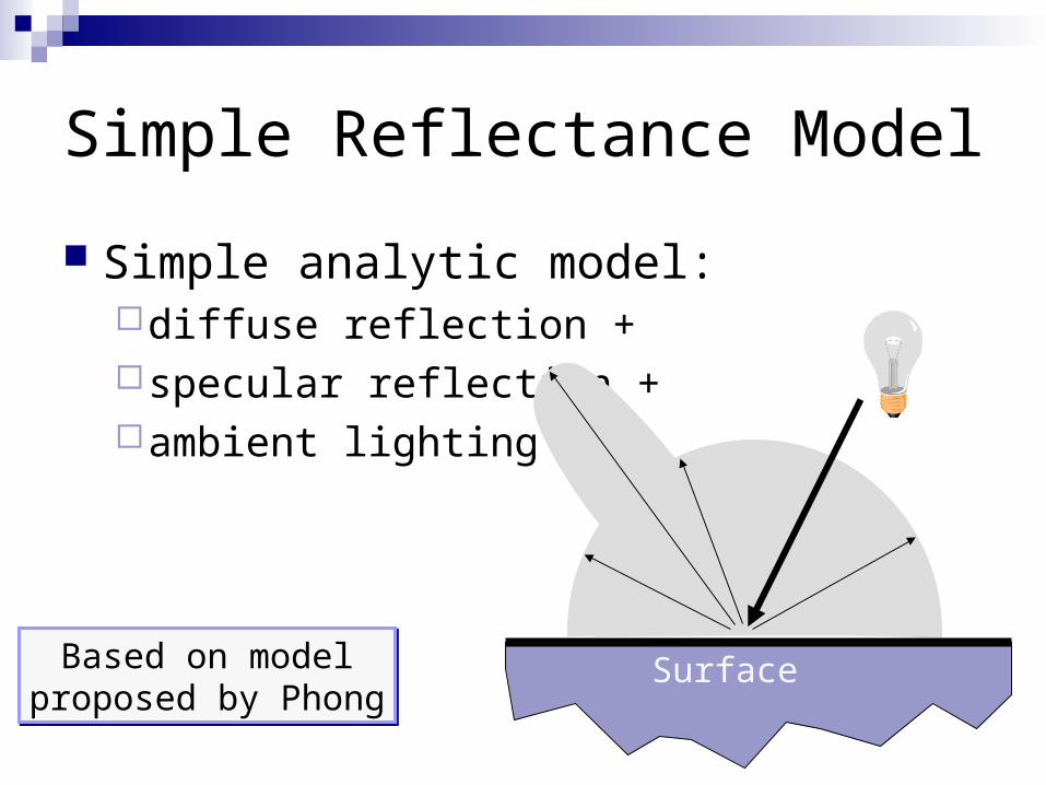
Simple Reflectance Model

Simple analytic model: diffuse reflection +specular reflection +ambient lighting

SurfaceBased on modelproposed by Phong

Based on modelproposed by Phong

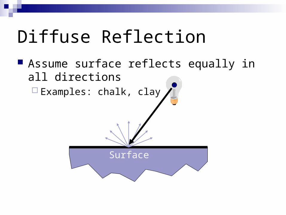
Diffuse Reflection Assume surface reflects equally in all directions

Examples: chalk, clay

Surface

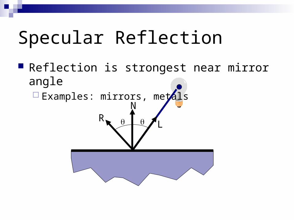
Specular Reflection

Reflection is strongest near mirror angle Examples: mirrors, metals

N

LR

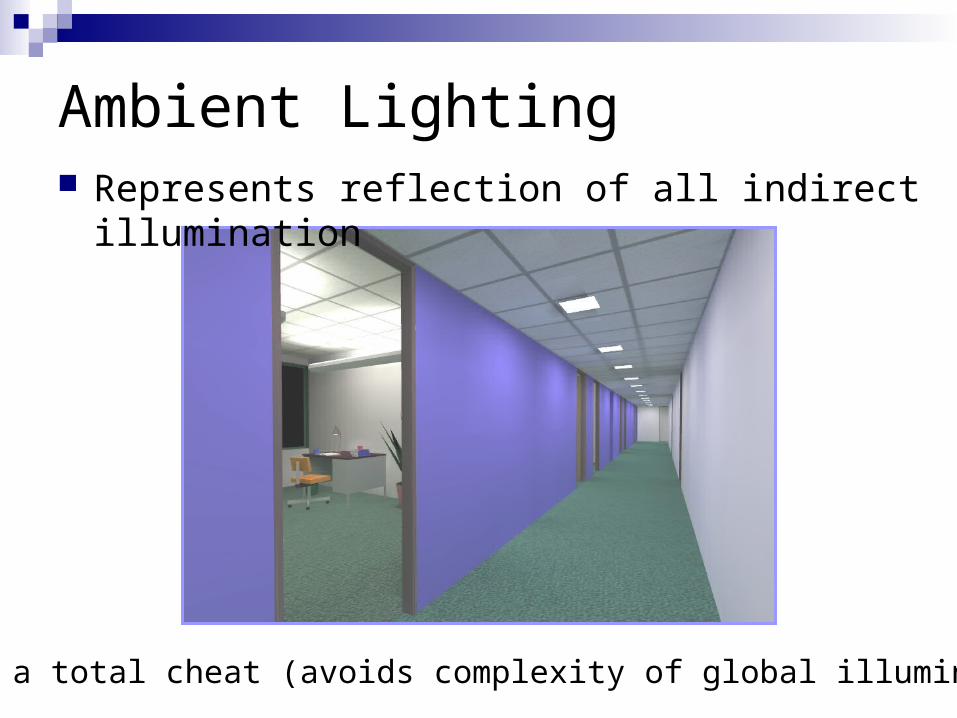
Ambient Lighting

This is a total cheat (avoids complexity of global illumination)!

Represents reflection of all indirect illumination

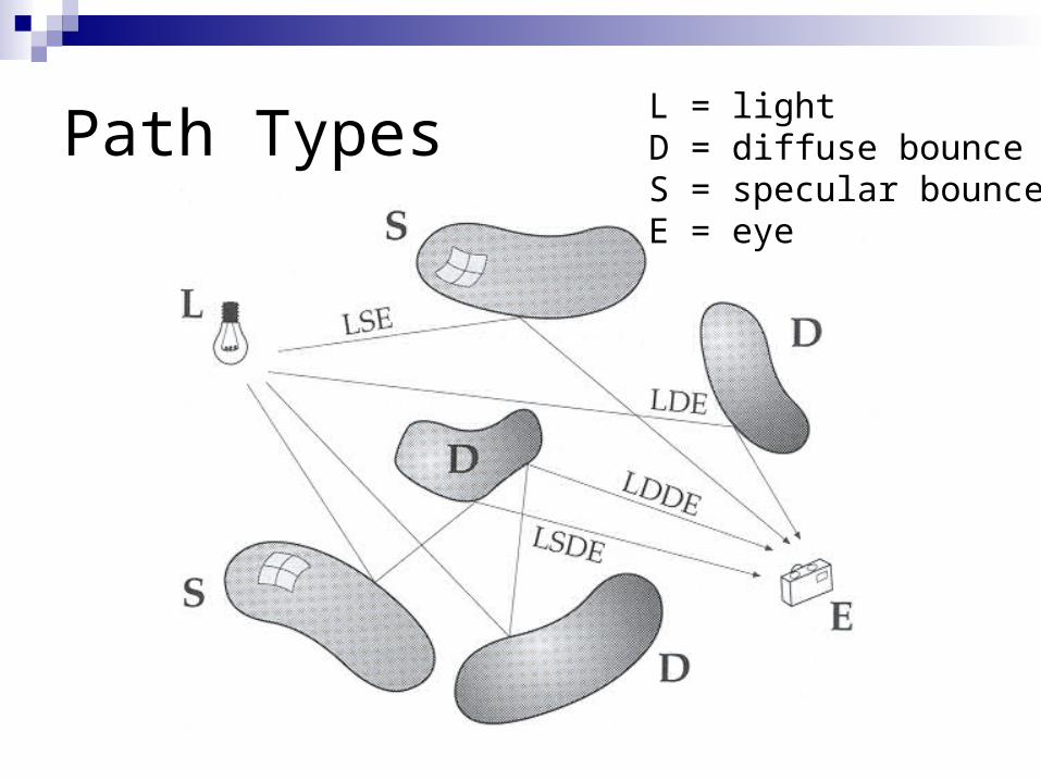
Path TypesL = lightD = diffuse bounceS = specular bounceE = eye

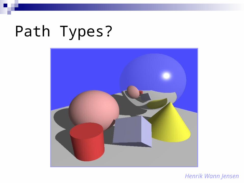
Path Types?

Henrik Wann Jensen

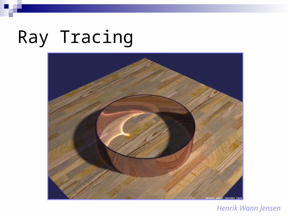
Ray Tracing

Henrik Wann Jensen

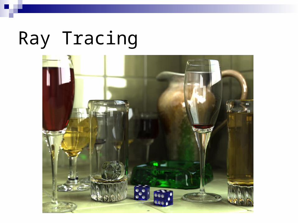
Ray Tracing

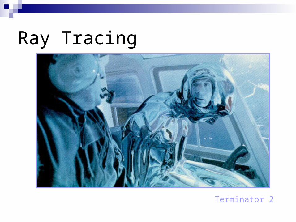
Ray Tracing

Terminator 2

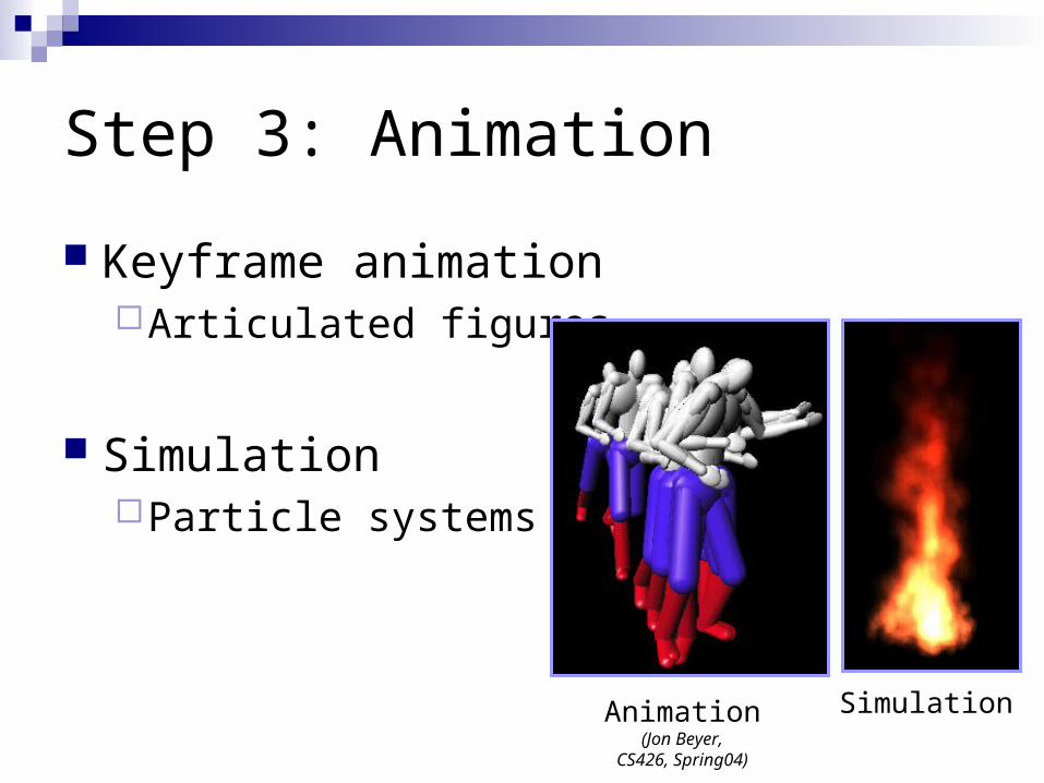
Step 3: Animation

Keyframe animationArticulated figures

SimulationParticle systems

Animation(Jon Beyer,

CS426, Spring04)

Simulation

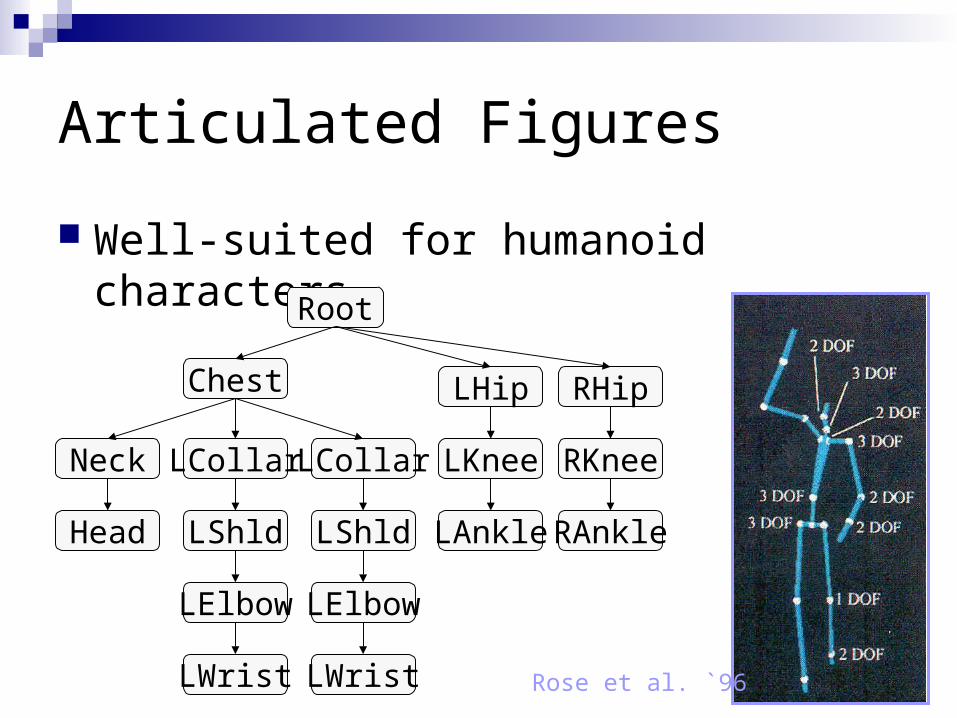
Articulated Figures

Rose et al. `96

Well-suited for humanoid characters

Root

LHip

LKnee

LAnkle

RHip

RKnee

RAnkle

Chest

LCollar

LShld

LElbow

LWrist

LCollar

LShld

LElbow

LWrist

Neck

Head

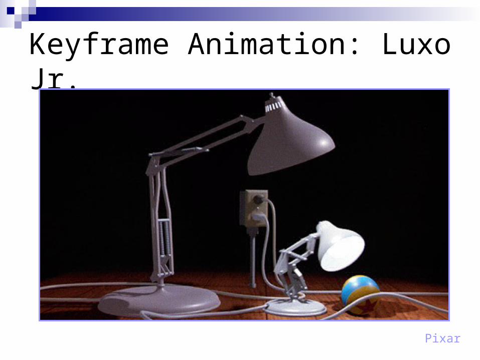
Keyframe Animation: Luxo Jr.

Pixar

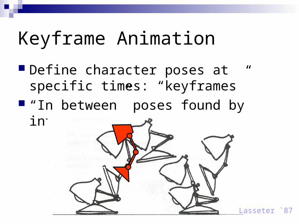
Keyframe Animation

Define character poses at specific times: “keyframes”

“In between” poses found by interpolation

Lasseter `87

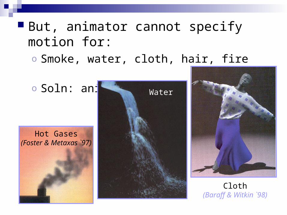
But, animator cannot specify motion for:o Smoke, water, cloth, hair, fire

o Soln: animation!

Cloth(Baraff & Witkin `98)

Water

Hot Gases(Foster & Metaxas `97)

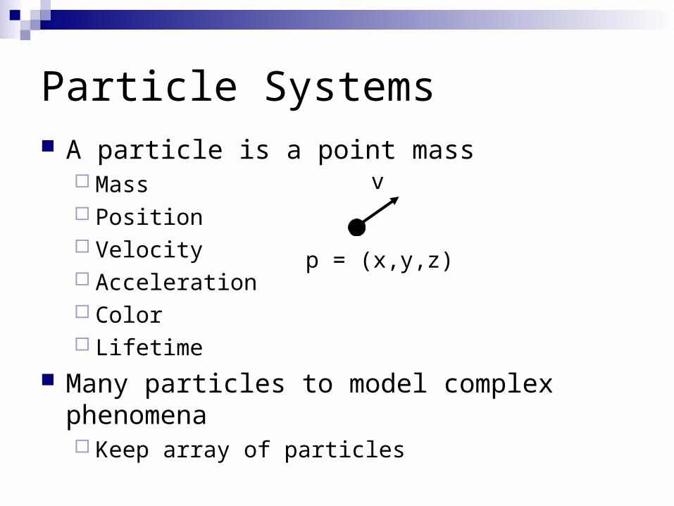
Particle Systems A particle is a point mass

Mass Position Velocity Acceleration Color Lifetime

Many particles to model complex phenomena Keep array of particles

p = (x,y,z)

v

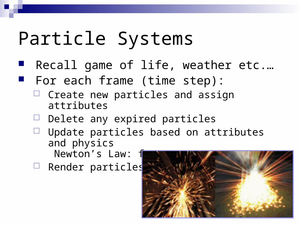
Particle Systems Recall game of life, weather etc.… For each frame (time step):

Create new particles and assign attributes Delete any expired particles Update particles based on attributes and physics

Newton’s Law: f=ma Render particles