Computer simulation of padaptive optical systems

Bolbasova L.A., Lukin V. P., Konyaev P.A. o baso a , u , o yae

V.E. Zuev Institute of Atmospheric Optics SB RASV.E. Zuev Institute of Atmospheric Optics SB RAS Tomsk, Russia

Short history of development of adaptive optics theory optics theory

• In 1986 I completed work at monograph (English translation) • Lukin V.P. Atmospheric Adaptive Optics. SPIE Press. 1996. p p p• which developed the theory of adaptive correction of laser beams and images in

the atmosphere as a turbulent, absorbing, and refractive medium. • A) aspects of two-color adaptive system• Lukin V.P. Efficiency of some correction systems // Optics Letters. 1979. V.4.

No.1. pp.15-17.• B) applying an artificial reference source (1979-1983) for image correction• Lukin V.P. Correction of random angular displacements for optical beams //

Quantum Electronics. 1980. V.7. №6. pp.1270-1279.• Lukin V.P., Matuchin V.F. An adaptive image correction // Kvantovaja

Electronika. 1983. V.10. No.12. pp.2465-2473.• C) dynamic characteristics of adaptive optical systems (1986), where the

ideas of “predicting” fluctuations for adaptive system operation were used for the first timethe first time

• Lukin V.P., Zuev V.E. Dynamic characteristics of optical systems // Applied Optics. 1987. V.27. No.1. pp.139-147.

The main elements of adaptive optics system simulation

Atmospheric path for propagation adaptive mirror

wavefrontwavefront sensor

1. Basic equationsq• Our 4-dimentional computer code based on the a set of parabolic

equations for wave propagation

,2)1(2)(2 2

2

2

2

2

ext EikEnkEyxz

Eik

with the boundary conditions for corrected beam and reference beam

,2)1(2)(2 22

2

2

2

rextrrr EikEnkE

yxzEik

with the boundary conditions for corrected beam and reference beam

),2

exp(),(),,,(22

cd ifyxikyxItozyxE

where corrected phase, is lag (delay) of )},,,({ tozyxEA rñ d

f),,,,(),,(),,,( tfzyxEtyxRtfzyxEr

control induced by adaptive system, is adaptive system operator, is coefficient of target reflection or Rayleigh backscattering, is

a coefficient of extinction of radiation.

dA

R ext

Structure of 4-dimentional numerical dynamic model of AOSdynamic model of AOS

In the period of 1991-1995 have beendeveloped four dimensional numericaldynamic model of atmospheric adaptivesystems.L ki V F B M d li f h iLukin V., Fortes B. Modeling of the imageobserved through a turbulent atmosphere //Proc SPIE 1992 V 1688 pp 477-488//Proc. SPIE. 1992. V.1688. pp.477 488.Fortes B.V., Kanev F.Yu., Konyaev P.A.,Lukin V.P. Potential capabilities of аdaptiveoptical systems in the atmosphere //Journ.Opt.Soc.Am.A. 1994. V.11. No.2.

903 907p.903-907.Lukin V., Fortes B. Adaptive beaming andimaging in the turbulent atmosphereimaging in the turbulent atmosphere. SPIE Press. PM109. 2002. 201 p.

Hartmann-Shack sensor simulation

Deformable mirror: Zernike basis and a set of response functions of DM

CHARACTERISTICS OF GROUND-BASED OPTICAL TELESCOPE DUE TO ATMOSPHERIC TURBULENCE

In 1994 we completed a design project ofan adaptive system for the 10-metercombined Russian telescope AST-10.

TELESCOPE DUE TO ATMOSPHERIC TURBULENCE

combined Russian telescope AST 10.Lukin V.P. Computer modeling of adaptiveoptics for telescope design // ESOWorkshop Proc. No.54, 1995, pp.373-378.p , , ppLukin V.P., Fortes B.V. Partial phasecorrection of turbulent distortions intelescope AST-10 // Applied Optics. 1998.V.37. №21. pp.4561-4568.Characteristics of long-base stellarinterferometers were calculated (1997)with allowance for the interferometer baseorientation, wind velocity distribution, andthe outer scale of turbulence.

ki V P B V G d b dLukin V.P., Fortes B.V. Ground-basedspatial interferometers and atmosphericturbulence //Pure and Applied Optics.1996 V5 N 1 1 111996. V.5. No.1. pp.1-11.

CHARACTERISTICS OF GROUND-BASED OPTICAL TELESCOPE DUE TO ATMOSPHERIC TURBULENCE

In 1994 we completed a design project ofan adaptive system for the 10-metercombined Russian telescope AST-10.

TELESCOPE DUE TO ATMOSPHERIC TURBULENCE

combined Russian telescope AST 10.Lukin V.P. Computer modeling of adaptiveoptics for telescope design // ESOWorkshop Proc. No.54, 1995, pp.373-378.p , , ppLukin V.P., Fortes B.V. Partial phasecorrection of turbulent distortions intelescope AST-10 // Applied Optics. 1998.V.37. №21. pp.4561-4568.Characteristics of long-base stellarinterferometers were calculated (1997)with allowance for the interferometer baseorientation, wind velocity distribution, andthe outer scale of turbulence.

ki V P B V G d b dLukin V.P., Fortes B.V. Ground-basedspatial interferometers and atmosphericturbulence //Pure and Applied Optics.1996 V5 N 1 1 111996. V.5. No.1. pp.1-11.

CHARACTERISTICS OF GROUND-BASED OPTICAL TELESCOPE DUE TO ATMOSPHERIC TURBULENCETELESCOPE DUE TO ATMOSPHERIC TURBULENCE

• Using an analytical algorithm for atmospheric g y g pcorrection the performance of the Euro50 telescope project is analyzed. Th t h i d l l d i th ORM• The atmospheric model employed is the ORM (Observatorio del Roque de los Muchachos) 7 layer model with an outer scale distribution.model with an outer scale distribution.

• The values of effective outer scale found that at apertures of modern telescopes of several meters the influence of the finite L0 on the energy balance between tip-tilt and higher order modes must be properly taken into accountproperly taken into account.

• Lukin V., Goncharov A., Owner-Petersen M., Andersen T.• The effective outer scale estimation for Euro-50 site • // Proc. SPIE. 2002. Vol.5026. pp.112-118.

Adaptive correction systems for the Baikal Solar Vacuum Telescope (2003-2012)p ( )

1- Sunspot 2- Pores group 3- Granulation

Contrast 25-30 % Contrast 1-3 %Contrast 10-15 %

C t id t ki lCentroid tracking analog

Centroid tracking digital 2.2

2.4

а с т,

%

Correlation tracking1.8

2.0

К о н т р а

0 200 400 600 800 1000

Последовательность кадров

Used correlation tracking algorithms

1 1

)()()(N M

mjliImlIjiC

1. Correlation function

I t f

0 0

),(),(),(l m

R mjliImlIjiC

2. Normalized correlation function

I – current frame

Ir – reference frame

2/11 12

1 12 )()()(

N MN M

mjliImlIjiC

RN CCC /

0 00 0),(),(),(

l m

Rl m

R mjliImlIjiC

l i l i h

RIFIFFC F – mixed radix FFT

3. Correlation FFT algorithm

)( kkHIFIFFC

4. Modified correlation FFT algorithm (Booster)

),( yxBRm kkHIFIFFC

Correlation tracking gof spot patterns

1E-4

X

1E-8

1E-6

1E-10Power spectrum of non-corrected (black) and corrected (red) image

1E-4 1E-3 0,01 0,1 f / f0displacement.

Modified correlation wavefront sensor (2006) is based on camera DALSA CА-D6 (260Х260 pixels, pixel size 10 mkm, 12 bit, 955 fpc)

200

250

300

200

250

300Comparison of joint

correlation functions for

50

100

150

50

100

150

200traditional (left) and modified (right) correlation trackers.

118 35 52 69 86

Р1

Р490

118 35 52 69 86

Р1

Р490

The set of pictures for ”short exposure”p p(2 мс), in regime of “long exposure” (2 с) without control, and in regime «long exposure» (2 с) with modified sensor.

3- Granulation

Solar tracking SystemsCountry USAUSA FranceFrance--

ItalyItalySpainSpain ChinaChina Russia Russia

BSVTBSVTYears of operation

1989 1995 1995 2001 2001-2005

Diameter 760 900 980 430 760Diameter (mm)

760 900 980 430 760

Beacon granulation granulation granulation Sunspot Sunspot/ granulationg

Algorithm cross correlation

granulation tracker

absolute difference

absolute difference

modified correlation

Sampling 417 582 1350 419 164-245Sampling freq (Hz)

417 582 1350 419 164 245

Field of view 10”x10” 2”x2” ~ 12”x12”

14”x14” 5”x5” ~ 20”x20”

33”x33”12 x12 20 x20

Bandwidth 25Open loop

60Close -3dB

100Open loop

84 open loop30 close -3dB

120Open loop

Image q alit Motion 0 023” Resol tion Motion 0 05” Motion 0 14” Motion 0 07”Image quality Motion 0.023” rms

Resolution 0.2”

Motion 0.05” rms

Motion 0.14” rms

Motion 0.07” rms

Present view of adaptive system ANGARA on the Big Solar Vacuum Telescope (Baikal Astrophysical Observatory, 2009)

RF patent on useful model «Telescope with adaptive optical system» № 111695 (priority at 29.06.2011, (p y ,IAO SB RAS, ISTP SB RAS)

19

Correlation S-H wavefront sensor

• This sensor use the extended object imagesas a source of measurement, as well as solarsports, pores, and solar granularities.

• Sensor consist from the raster of squarediffractive lenses with numerical aperturediffractive lenses with numerical aperture0.019 and video-camera GE680 Prosilica(Canada) with resolution 640х480 pixels(size of 1 pixel is 7 4 m)(size of 1 pixel is 7.4 m).

• This device is suitable to measure wavefrontdistortions with error below 1/60 ofwavelength.

• Wave-front sensor of FOW not more than• 40 arc sec• 40 arc. sec.• Botygina N.N., Emaleev O.N., Konyaev

P.A., Lukin V.P. Wavefront sensors for adaptive optical systems //Measurement Science Review. 2010. V.10. №3. P.101.

Deformable mirror /adaptive system ANGARA

Amplifier, one channel

Bymorph mirrorBymorph mirror

Mirror , back view

Base of АОS simulation – technologies of parallel programming

Set-ups for parallel programming:INTEL Math Kernel Library (MKL) v.10.3INTEL Integrated Performance Primitives (IPP) v.7.0NVIDIA CUDA Toolkit 4.01

Basic functions of library MKL:

Methods and features of parallel algorithms fornumerical simulation of optical wavespropagation are considered The scalarBasic functions of library MKL:

Vector and matrix algebraStatistics and random number generatorsFast Fourier Transformation (1-D, 2-D, 3-D)

Basic libraries of IPP:Si l i ( l ti l ti )

propagation are considered. The scalarparabolic equation for a complex amplitude ofmonochromatic waves was solved numerically,

Signal processing (convolution, correlation)Images processing (filtration, digital transformations, coding and decoding)

Basic functions of library CUDA:Vector and matrix algebra

using the Fourier transform method forhomogeneous media and split-step Fouriermethod for inhomogeneous media

Statistics and random number generatorsFast Fourier Transformation (1-D, 2-D, 3-D) 2 2

212 22 [ 2 ( , , )] 0Uik k n x y z U

z x y

method for inhomogeneous media.

Two parallel algorithms using[ ]D R

U L L Uz

2 2

2 2[ ] _2DiL diffraction operatork x y

1( , , ) _RL ikn x y z refraction operator Two parallel algorithms, using OpenMP technology with MKL library for Intel multicore

2k x y

Konyaev P.A., Tartakovskii E.A., Filimonov G.A. Computer simulation of optical waves propagation,

i ll l i t h i // At h i

processorsand CUDA technology for NVIDIA using parallel programming technique // Atmospheric

and Oceanic Optics. 2011. V. 24, No.05. P. 359-365 [in Russian].

CUDA technology for NVIDIA graphic acceleratorshave been created.

The hardware system for computer simulation is an off-the-shell

desktop with6- core 12-thread Intel Core i7-980 atth i f f 3 6 Ghthe maximum frequency of 3.6 GhzTurbo boost and an NVIDIAGeForce GTX 590 graphicGeForce GTX 590 graphicaccelerator with 1024 universalprocessors operating at 1.5 Ghz.• Model SIMD (one team – many

data, graphic memory 3000 Mb)Interface OpenMP (Intel) and CUDAInterface OpenMP (Intel) and CUDA(Compute Unified DeviceArchitecture).)OS Linux, Windows, MS VisualStudio, NVIDIA CUDA Toolkit 4.x, plugin for MATLAB

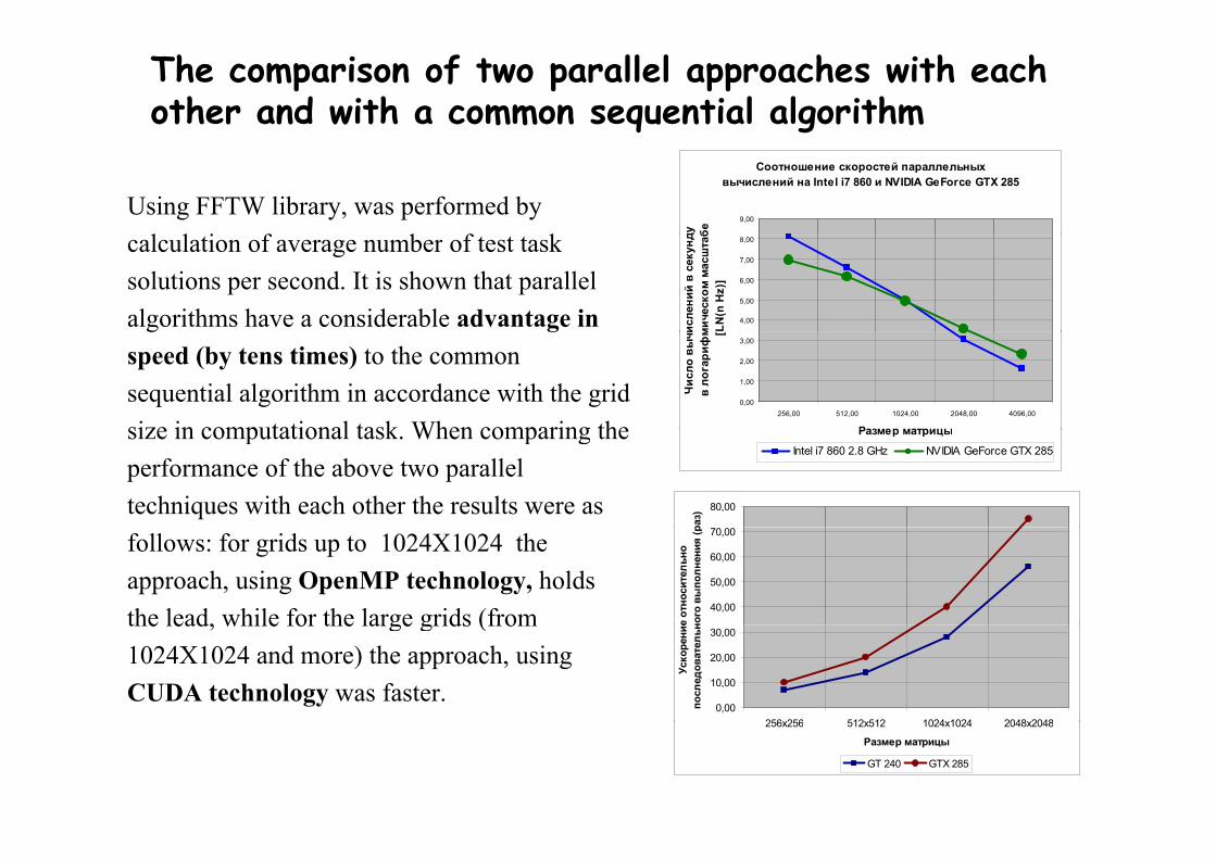
The comparison of two parallel approaches with each other and with a common sequential algorithm

Using FFTW library, was performed byl l i f b f k

Соотношение скоростей параллельных вычислений на Intel i7 860 и NVIDIA GeForce GTX 285

9,00

ду

бе

calculation of average number of test tasksolutions per second. It is shown that parallelalgorithms have a considerable advantage in 4,00

5,00

6,00

7,00

8,00

исле

ний в секунд

мич

еско

м масштаб

LN(n

Hz)

]

g gspeed (by tens times) to the commonsequential algorithm in accordance with the gridsize in computational task When comparing the

0,00

1,00

2,00

3,00

256,00 512,00 1024,00 2048,00 4096,00

Размер матрицы

Чис

ло вычи

в ло

гари

фм [

size in computational task. When comparing theperformance of the above two paralleltechniques with each other the results were as

Размер матрицы

Intel i7 860 2.8 GHz NVIDIA GeForce GTX 285

80,00

раз)

follows: for grids up to 1024Х1024 theapproach, using OpenMP technology, holdsthe lead, while for the large grids (from 40,00

50,00

60,00

70,00

е отно

ситель

но

ного

выпо

лнения

(р

the lead, while for the large grids (from1024Х1024 and more) the approach, usingCUDA technology was faster.

0,00

10,00

20,00

30,00

256x256 512x512 1024x1024 2048x2048

Ускорени

епо

след

овател

ьн

256x256 512x512 1024x1024 2048x2048

Размер матрицы

GT 240 GTX 285

Turbulence with large scales of sizes

• Spectral method (2-D FFT MKL, CUDA, IPP): SIMD-oriented fast Mersenne TwisterSpectral method (2 D FFT MKL, CUDA, IPP):• - model of turbulence with large scales of sizes ~1:10000• - modern generators of uncorrelated numbers with large period

(linear congruent sensor from standard library ~ 2^31-1)• - simulation of large scale optics with high resolution

random generator SFMT19937(Intel MKL) with period =2^19937

simulation of large scale optics with high resolution• - dynamic model of turbulence for AOS modeling

8192

256

8192

Correlation S-H wavefront sensor portal for solar telescope

Measurements of wavefront: S-H wavefront sensor• Technology of CUDA Batched Processing (extended model of gy g (

SIMD)• Parallel algorithms of Hatrmannograms processing

– Two-dimentional correction with parallel 2-D FFT,P ll l lti li ti t b t ti t i– Parallel multiplication vector by reconstruction matrix

– Parallel algorithm of Fourier demodulation• Modeling of extremal wave-front sensors

Parallel programming technique for computer simulation of optical waves propagation

A modified spectral-phase algorithm forp p gcomputer simulation of time-evolving turbulence inatmospheric and adaptive optics applications

Known spectral-phase method for computer simulation of random processesand fields with given spectral densities. For 2-D discrete field this method mayto present as

1 1

( , ) ( , ) exp exp 2( , )L M

l i mjs i j S l m g l mL M

ii

0 0

( ) ( ) p p( , )l m

j gL M

( , ) exp .( , )FFT S l m g l m i

Here FFT is operator of discrete Fourier transformation, g(l, m) is a 2-Drandom field (“white noise”); S(l m) is spectral amplitude satisfyingrandom field ( white noise ); S(l, m) is spectral amplitude, satisfyingcondition

2 2 2 2, , ,( ) , ,l m l m l mS k k k k l m

where Ф(kl, m) is required spectral density.

, , ,

As a model of evolution of field s(k, l) in time for discrete moments of time T h T i i t l t li d th d l f t itn = nT, where T is interval to sampling used the model of autoregression

with slitherring average, which is broadly used in theories of the random processes.Very interesting model of 1-order, which present minimum requirements to memory of computer:

1( ) ( ) ;( 1)f nT a f z nTn T

Here r(nT) is descrete white noise with normal distribution, zero average

1( ) ( ) .( 1)z nT b r r nTn T Here r(nT) is descrete white noise with normal distribution, zero average and variance. Figure below present evolution of 2-D random field s(i, j) with Kolmogov’s power type of model with coefficients a1 = 0.999, b1 = 0 9 and varience of noise s2 = 0 01 The sequence of the framesb1 = 0.9 and varience of noise s2 = 0.01. The sequence of the frames illustrates the fluent time histories, comparing first and the last frames to serieses, possible notice that occurred full change the initial frame.

• For modeling of the evolutions in media, moving at the speed of V(Vх, Vy), g , g p ( , y),necessary introduct exponential multiplier of the shift:

( )( ) exp exp( ) nT v vs i j FFT S g l m ii• Evolution of the field is shown on Figure with same power spectrum in moving

(left to right) media.

( )( , ) exp exp .( , ) x ynT v vs i j FFT S g l m ii

( g )

• The implementation of the algorithm is shown to be simple and efficient in simulations of dynamic be simple and efficient in simulations of dynamic problems of atmospheric and adaptive optics

Hardware-programme complex for Full Sun Telescope of Baikal Astrophysical Observatoryof Baikal Astrophysical Observatory

Complex for numerical processing and analysis of images of solarchromosphere on the base of modern technologies of parallel programmingchromosphere on the base of modern technologies of parallel programming

• List of problems• analysis of images and choose the best image in different formats and• - analysis of images and choose the best image in different formats and

transformations,• - correction of instrumentation and atmospheric distortions, calibration, and

high precision co-ordination of images,high precision co ordination of images, • - spherical transformation details on Sun surface with scale changing,

measure of angular of rotation, coefficient of scaling, • - corrtensial transformation of images – поворот, масштабирование,corrtensial transformation of images поворот, масштабирование,

перенос и т.д.,• - space-temporal correlation and spectral analysis of images.The features given hardware-programme complex do its irreplaceable atThe features given hardware programme complex do its irreplaceable atdecision of the problems solar physicists. It also can be used for processingexisting database of the observations Baykal Astrophysical Observatory thatwill enable to get generalising given on perennial observations Sunwill enable to get generalising given on perennial observations Sun.

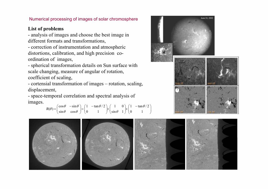
Numerical processing of images of solar chromosphere

List of problemsList of problems- analysis of images and choose the best image in different formats and transformations,- correction of instrumentation and atmospheric di i lib i d hi h i idistortions, calibration, and high precision co-ordination of images, - spherical transformation details on Sun surface with scale changing, measure of angular of rotation, sca e c a g g, easu e o a gu a o o a o ,coefficient of scaling, - cortensial transformation of images – rotation, scaling, displacement,

t l l ti d t l l i f

cos sin 1 tan / 2 1 0 1 tan / 2( )

sin cos 0 1 sin 1 0 1R

- space-temporal correlation and spectral analysis of images.

Picture frame of HPC

Dynamic characteristics of adaptive systemsy p y

• A common adaptive system with a finite frequency band (or a finite response time) is described as a dynamic constant time-delay systemresponse time) is described as a dynamic constant time delay system, where time delay is to be much shorter than the time of coherence radius transfer through an telescope aperture by a mean wind speed.

• The questions of the image formation are considered with use the reference q gsource.

• The analytical calculation of the Strehl parameter is made on base of the generalized principle of Huygens–Kirchhoff.

• An adaptive system is considered, where the correcting phase is calculated with the use of both its derivatives and the signal, as well as adaptive systems using different time predicting algorithms of correcting signal for future time pointsfuture time points.

• The use of a predicted phase front of the correcting wave allows much longer time delays.

• The stronger phase distortions in the optical wave the higher time gain in• The stronger phase distortions in the optical wave the higher time gain in comparison with common (with constant time-delay) adaptive system.

Development of algorithms of forecasting correctionPhase fluctuation evolution on small time interval presented as a truncated Taylor’sPhase fluctuation evolution on small time interval presented as a truncated Taylor s expansion:

!2/)()()()( 2 tttStS SS

r1. Traditional scheme of correction

!2/),(),(),(),( tttStS SS

),(),( tStS

6/10

01 )/2)((53.0 rR

vr

12/7

00

2 )/2)((59.0 rRvr

2. “Fast” correction

vtvStStS 0),(),(),( v

12/5012 )/2(/ rR

Algorithms of forecasting correction

Ph fl t ti l ti ll ti i t l t d t t dPhase fluctuation evolution on small time interval presented as a truncated Taylor’s expansion:

2

3 Correction with acceleration

!2/),(),(),(),( 2 tttStS SS

!2/),(),(),(),( 220

20 vtSvtStStS

3. Correction with acceleration

36/5023 )/2(/ rR

4. Correction on the base of “frosen fluctuations” model

)()(ˆ SS ),(),( 0 tvrStrS )/(/ 014 vv

2/1*)2*][( 0vv

Variances of residual error of wavefront estimation as a function of intensityof turbulent distortions for different temporal delay (curves 1-3), 4 – without forecasting.

Spectral characteristics of adaptive systemsSpectral characteristics of adaptive systems