Computer Sciences Department -...

Computer Sciences Department

Broadening the Applicability of Relational Learning Trevor Walker Technical Report #1698 September 2011

Broadening the Applicability of

Relational Learning

by

Trevor Walker

A Dissertation submitted in partial fulfillment of

the requirements for the degree of

Doctor of Philosophy

(Computer Sciences)

At the

UNIVERSITY OF WISCONSIN-MADISON

2011

i

ACKNOWLEDGMENTS

Thanks to my advisor, Jude Shavlik, to my collaborators Lisa Torrey, Rich Maclin, Sriraam

Natarajan, and Gautam Kunapuli, to my committee members, and to the Machine Learning Group at the

University of Wisconsin-Madison. Special thanks to Lisa for all the good years as my office mate. This

research was partially supported by DARPA grants HR0011-04-1-0007, HR0011-07-C-0060, and

FA8650-06-C-7606.

DISCARD THIS PAGE

iii

TABLE OF CONTENTS

ACKNOWLEDGMENTS ........................................................................................................ i

TABLE OF CONTENTS ....................................................................................................... iii

LIST OF TABLES ................................................................................................................. vii

LIST OF FIGURES ................................................................................................................. x

LIST OF ALGORITHMS ................................................................................................... xix

ABSTRACT .......................................................................................................................... xxi

1 Introduction ........................................................................................................................ 1

1.1 Motivation ...................................................................................................................... 2 1.2 Contributions .................................................................................................................. 6 1.3 Thesis Statement ............................................................................................................. 7 1.4 Thesis Overview ............................................................................................................. 8

2 Background ......................................................................................................................... 9

2.1 First-Order Logic ............................................................................................................ 9 2.1.1 Unification ........................................................................................................... 11 2.1.2 Horn Clauses and Selective Linear Definite (SLD) Resolution .......................... 11

2.2 Supervised Learning ..................................................................................................... 14 2.2.1 Classification Versus Regression ......................................................................... 16 2.2.2 Fixed-Length Feature Vectors Versus Relational Feature Description. .............. 18 2.2.3 Inductive Logic Programming ............................................................................. 19 2.2.4 Support Vector Machines .................................................................................... 28 2.2.5 Boosted Relational Dependency Networks.......................................................... 31

2.3 Reinforcement Learning ............................................................................................... 33 2.3.1 Task Definition .................................................................................................... 34 2.3.2 Optimal Policies and the Bellman Equations ....................................................... 37 2.3.3 Common Reinforcement Learning Approaches .................................................. 38

3 Testbeds ............................................................................................................................. 44

3.1 Bootstrap Learning ILP Tasks ...................................................................................... 44 3.1.1 Unmanned Arial Vehicle Domain ....................................................................... 46 3.1.2 The Armored Task Force Domain ....................................................................... 47

3.2 Wargus Real-Time Strategy Tasks ............................................................................... 47 3.3 Standard ILP Tasks ....................................................................................................... 49

3.3.1 Advised-By ILP Task .......................................................................................... 49 3.3.2 Carcinogenesis ILP Task ..................................................................................... 49 3.3.3 Mutagenesis ILP Task ......................................................................................... 50

3.4 RoboCup Simulated Soccer Reinforcement Learning Domain .................................... 51

iv

4 Generation of Background Knowledge from Advice about Specific Examples .......... 55

4.1 Converting Advice to Background Knowledge ............................................................ 60 4.1.1 Generalizing Advice ............................................................................................ 61 4.1.2 Standarizing Advice ............................................................................................. 67 4.1.3 Generating Background Rules ............................................................................. 67 4.1.4 Priority and Mode Assignment ............................................................................ 69

4.2 Experimental Results .................................................................................................... 72 4.2.1 Methodology ........................................................................................................ 73 4.2.2 Results .................................................................................................................. 73 4.2.3 Discussion ............................................................................................................ 77

4.3 Related Work ................................................................................................................ 78 4.4 Conclusions and Future Work ...................................................................................... 79

5 Advice Acquisition via a Human-Computer Interface .................................................. 81

5.1 Overview of Approach ................................................................................................. 82 5.2 Intelligence, Surveillance and Reconnaissance – A Motivating Application ............... 84 5.3 Our Advice-Taking HCI ............................................................................................... 85

5.3.1 Elements of our Advice-Taking HCI ................................................................... 87 5.3.2 A General HCI implementation ........................................................................... 90

5.4 Generating Generalized Advice and Learning with It .................................................. 92 5.5 HCI for Reviewing Learned Models ............................................................................ 92 5.6 Experimental Results .................................................................................................... 94

5.6.1 Methodology ........................................................................................................ 96 5.6.2 Results .................................................................................................................. 98 5.6.3 Discussion .......................................................................................................... 100

5.7 Background and Related Work ................................................................................... 101 5.8 Conclusions and Future Work .................................................................................... 102

6 The ONION – Automatic Parameter Tuning for Inductive Logic Programming ...... 103

6.1 Layered Approach to Parameter Tuning..................................................................... 105 6.2 Exploiting Relevance .................................................................................................. 109 6.3 Parameters to Tune ..................................................................................................... 111

6.3.1 MinimumTheoryPrecision Parameter ................................................................ 112 6.3.2 MaximumSearchNodes Parameter ..................................................................... 113 6.3.3 RelevanceStrength Parameter ............................................................................ 113 6.3.4 MaximumClausesInTheory Parameter .............................................................. 113 6.3.5 MaximumClauseLength Parameter ................................................................... 114 6.3.6 LearnNegatedConcept Parameter ...................................................................... 116

6.4 Experimental Results .................................................................................................. 116 6.4.1 Methodology ...................................................................................................... 117 6.4.2 Results ................................................................................................................ 120 6.4.3 Discussion .......................................................................................................... 123

6.5 Why the ONION is Needed .......................................................................................... 124 6.5.1 Methodology ...................................................................................................... 124 6.5.2 Results ................................................................................................................ 125 6.5.3 Discussion .......................................................................................................... 132

6.6 Related Work .............................................................................................................. 132

v

6.7 Conclusions and Future Work .................................................................................... 133

7 Additional Explorations – Building Relational World Models .................................. 134

7.1 Building World Models .............................................................................................. 136 7.1.1 Terminology....................................................................................................... 137 7.1.2 Algorithm Overview .......................................................................................... 138 7.1.3 Preimage Selection ............................................................................................ 139 7.1.4 Learning Concepts via ILP ................................................................................ 141 7.1.5 Building the A-MDP .......................................................................................... 142 7.1.6 The RL Learning Cycle ..................................................................................... 144

7.2 Experiments ................................................................................................................ 145 7.2.1 Methodology ...................................................................................................... 145 7.2.2 Results ................................................................................................................ 147 7.2.3 Discussion .......................................................................................................... 148

7.3 Related Work .............................................................................................................. 149 7.4 Conclusions and Future Work .................................................................................... 150

8 Additional Explorations – Building Relational Macros for Transfer in Reinforcement

Learning ...................................................................................................................................... 152

8.1 Related Work in Transfer Learning ............................................................................ 153 8.2 Executing a Relational Macro .................................................................................... 155 8.3 Learning a Relational Macro ...................................................................................... 156

8.3.1 Structure Learning ............................................................................................. 158 8.3.2 Ruleset Learning ................................................................................................ 159

8.4 Transferring a Relational Macro ................................................................................. 163 8.5 Experimental ............................................................................................................... 164

8.5.1 Methodology ...................................................................................................... 164 8.5.2 Results ................................................................................................................ 164 8.5.3 Discussion .......................................................................................................... 166

8.6 Conclusions and Future Work .................................................................................... 168

9 Conclusions ..................................................................................................................... 169

References ............................................................................................................................ 172

Nomenclature ....................................................................................................................... 179

DISCARD THIS PAGE

vii

LIST OF TABLES

Table 1.1. Overview of thesis chapters. ........................................................................................................................ 8

Table 2.1. Horn clause nomenclature. ........................................................................................................................ 13

Table 2.2. Categories of supervised learning algorithms. ........................................................................................... 16

Table 2.3. Sample grandparent ILP task setup. .......................................................................................................... 21

Table 2.4. Mode specifications. .................................................................................................................................. 26

Table 2.5. MDP parameter values for sample Maze task. .......................................................................................... 37

Table 3.1. Number of facts per lesson. This table lists the number of ground facts that have ILP modes, broken

down by both domain and task. .............................................................................................................. 45

Table 3.2. Features describing the tower defense world. .......................................................................................... 48

Table 3.3. Predicates available for the “theories tower will stand” predication task. ............................................... 49

Table 3.4. Advised-by ground facts (over all examples). ............................................................................................ 49

Table 3.5. Carcinogenisis ground facts (over all examples). ....................................................................................... 50

Table 3.6. Carcinogenesis background knowledge. .................................................................................................... 50

Table 3.7. Mutagenesis ground facts (over all examples). ......................................................................................... 51

Table 3.8. Mutagenesis background knowledge. ....................................................................................................... 51

Table 3.9. RoboCup task features. Arguments with capitol letters are logical variables. A complete list of task

features is generated by replacing variables with all appropriate constants. The ClosestTaker refers to

the taker closest to the keeper currently holding the ball. Likewise, the ClosestDefender refers to the

defender closest to the attacker currently holding the ball. ................................................................... 54

Table 4.1. ReadyToFly concept. Training data includes two examples, one positive, one negative, along with three

pieces of teacher provided advice, two pieces for the first example and one for the second. .............. 61

Table 4.2. Direct and indirect anti-substitutions. Direct anti-substitutions generalize equivalent terms to the same

variable. Indirect anti-substitutions generalize equivalent terms to different variables. ...................... 65

viii

Table 4.3. Generated Background Knowledge. Three types of background knowledge are created during advice

processing: per-piece, per-example, and mega-rule background knowledge. Per-piece is composed of

single pieces of advice. Per-example is composed of all advice piece for a single example. Mega-rules

use all provided advice combined via various logical operators. ............................................................ 69

Table 4.4. Several possible background knowledge heads for the same rule body. .................................................. 70

Table 5.1. Generated background knowledge for some simple ground advice. Initial ground advice is first

generalized. Then various combinations are generated representing possible guesses at the meaning

of the set of advice statements. .............................................................................................................. 93

Table 5.2. General statistics gleaned from the natural language advice provided by the users. ............................... 96

Table 5.3. The seven sentences of advice used. ......................................................................................................... 96

Table 5.4. Sample ground logical statements about the Wargus tower-defense game for one positive (pos1) and

one negative example (neg1). ................................................................................................................. 97

Table 5.5. Hand-written advice about the Wargus tower-defense game. The actual advice submitted to the ILP

system consisted of seven Horn clauses directly representing the hand-written advice. ...................... 98

Table 6.1. Relevance Strengths and associated meanings, listed in order of their relative strengths. .................... 111

Table 6.2. Primary and secondary parameters tuned through the ONION. ............................................................... 112

Table 6.3. Parameter settings tried during grid search and ONION experiments. ..................................................... 117

Table 6.4. Dataset sizes for ONION versus grid-search experiments. ........................................................................ 118

Table 8.1. BreakAway task features. Arguments with capitol letters are logical variables. A complete list of task

features is generated by replacing variables with all appropriate constants. The ClosestDefender

refers to the defender closest to the attacker currently holding the ball. ............................................ 160

DISCARD THIS PAGE

x

LIST OF FIGURES

Figure 2.1. Illustration of Supervised Learning. Given training data, a supervised learning algorithm learns a

function. The function, given a new feature description, predicts a label. ............................................ 15

Figure 2.2. A Classification supervised learning task. Positively and negatively labeled examples exist in some

feature space. A supervised learning algorithm attempts to learn a function that separates the

positively labeled examples from the negatively labeled ones. The learned boundary between the

positive and negative examples is called the decision boundary. ........................................................... 17

Figure 2.3. A Regression supervised learning task. Numerically labeled examples exist in some feature space. A

supervised learning algorithm attempts to learn a function – the dashed line above – predicting the

values of unseen points in the feature space. ........................................................................................ 18

Figure 2.4. Illustration of ILP learning and evaluation process. During learning, the ILP algorithm uses training data

in the form of positive and negative logical formulas, along with a set of background knowledge, to

learn a logical theory. During evaluation, the logical theory, along with background knowledge,

predicts the label of new examples. ........................................................................................................ 20

Figure 2.5. Illustration of ILP learning based upon SLD resolution. Learned theories are composed of multiple

definite clauses. An outer theory-learner repeatedly calls an inner clause-learner in order to assemble

the learned theory. .................................................................................................................................. 22

Figure 2.6. Illustration of an ILP search for a learned clause. The clause learner generates candidate clauses,

arranged in a tree structure, using the literals specified by the user. At each step, the clause is scored

against the positive and negative examples. The score determines when the search should stop as

well as controlling the order of the search. The numbers indicate the order in which the clause learner

searched the clauses. .............................................................................................................................. 24

Figure 2.7. Candidate clause in ILP search. The arguments of the literals are either “inputs” or “outputs”,

consuming and introducing variables, respectively. The dotted lines illustrate the connection between

outputs and inputs. ................................................................................................................................. 26

xi

Figure 2.8. An is-a hierarchy. The types of objects form a tree where sub-trees represent subtypes of the parent

type. ......................................................................................................................................................... 27

Figure 2.9. Illustration of the maximum-margin decision boundary. The maximum-margin decision boundary

maximizes the margin between the boundary and the closest training examples. Other decision

boundaries exist that perfectly separate the training examples but do not maximize the margin. ....... 29

Figure 2.10. Transformation of the feature space. In the original feature space (left), no linear decision boundary

separates the positive examples from the negative examples. In the transformed feature space (right),

created by applying transformation θ, the examples are linearly separable. ......................................... 29

Figure 2.11. A logical decision tree representing a conditionally probability distribution for determining the

probability a given tower falls. Each interior node is a logical decision point, with the left branch

representing a true evaluation and the right branch a false evaluation. Leaves represent output

potentials that must be normalized (see Equation 2.10) to produce the output probability. ................ 33

Figure 2.12. Reinforcement-learning environment-agent interaction. An agent receives state information from the

environment. Based upon that information, the agent chooses an action to perform. The

environment determines the outcome of performing the indicated action and presents the agent with

a reward and updated state information. ............................................................................................... 35

Figure 2.13. A sample maze reinforcement-learning task. The agent must discover a path through the maze to the

exit. A large positive reward is received when the exit is reached and a small negative reward is

received for each action taken. ............................................................................................................... 36

Figure 2.14. Taxonomy of some reinforcement learning approaches. ...................................................................... 39

Figure 2.15. Example of the Q-function for a maze task. For each state in the maze, each action has an associated

Q-value, representing the expected non-discounted reward received for taking that action (and

following the policy afterwards). The Q-values shown are the reward values after the Q-function has

converged to the optimal values. ............................................................................................................ 41

Figure 3.1. The UAV domain’s task hierarchy. The overall goal is to train an Unmanned Aerial Vehicle (UAV) to

perform Intelligent Surveillance and Reconnaissance (ISR). The expanded nodes represent by-example

xii

lesson, while the small boxes represent lesson taught via other methods. In some nodes “Int” is used

as shorthand for “Interestingness.”......................................................................................................... 46

Figure 3.2. Wargus Tower Defense Game. Multiple attacking units, consisting of swordsmen, archers, and ballista,

attack a defender’s tower. Depending on the composition of the attacking force, the two may survive

or be destroyed. The Wargus tower-defense learning task involves predicting which of these

outcomes will occur. ................................................................................................................................ 48

Figure 3.3. RoboCup soccer tasks. Several reinforcement learning task have been designed for the RoboCup

soccer simulator. Three such tasks are shown here. .............................................................................. 52

Figure 4.1. An illustration of a top-down ILP search for a inference rule to predict the literal predicate, whose

definition is the conjunction of literals q through z. Finding a long clause such as this can be quite hard,

but if a teacher gives advice (possibly across multiple examples) that the conjunction of literals q

through y is relevant, then finding the correct definition is much easier. .............................................. 59

Figure 4.2. Processing of sample advice by GENERATEBACKGROUNDKNOWLEDGE algorithm. Advice is transformed

through a series of phases, first generalizing individual advice statements, then standardizing variables

that occur in the target concept literal, and finally generating new background knowledge consisting of

various combinations of the individual advice pieces. Line numbers refer to those in Algorithm 4.1.

The generation of modes and priorities is not shown. ............................................................................ 64

Figure 4.3. Experiment A: Testset accuracy as a function of the number of training, with and without advice,

averaged over 14 tasks. ........................................................................................................................... 74

Figure 4.4. Experiment B: Impact of errors of omission in advice. The x axis indicates the probability value used in

the advice-removal process (see text). .................................................................................................... 75

Figure 4.5. Experiment C: The impact of mislabeled examples under various conditions. The x-axis indicates the

percentage of training data that is mislabeled. ...................................................................................... 77

Figure 5.1. Our human-computer learning paradigm. Initially the user specifies advice through an HCI. Then the

advice is processed and learning occurs. Afterward the results are presented to the user via an

evaluation HCI. The process iterates until the user is satisfied with the results. ................................... 83

xiii

Figure 5.2. Intelligence, surveillance and reconnaissance (ISR) learning and usage scenario. During the “learning

phase” an analyst categories interesting images and provides advice through an HCI to train a

probabilistic model. In the “real-world use” phase, the model sorts and filters incoming images

according to the probability the are interesting, presenting the most interesting images to the analyst.

The analyst then dispatches reconnaissance appropriately. ................................................................... 86

Figure 5.3. The Wargus tower-defense task. Multiple attacking units, consisting of swordsmen, archers, and

ballista, assault the defender’s tower. Depending on the composition of the attacking force, the tower

will survive or be destroyed. The Wargus tower-defense learning task involves predicting which of

these outcomes will occur. ...................................................................................................................... 87

Figure 5.4. Prototype GUI for advice taking in Wargus. The GUI consists of four sections: (upper-left) entity

selection and naming, (upper-right) display of current game board, (lower) controls specifying

relations between selected entities, and (not shown) a list of previously specified advice. .................. 88

Figure 5.5. Sketch of a general ILP advice-giving HCI. One area of the GUI (top) displays a graph of relations known

about an example, while the another area (bottom) allows the user to construct advice by dragging

relations from the relation graph. While not optimal for all domains, this general HCI would enable

advice to be provided without the creation of task-specific GUI. ........................................................... 91

Figure 5.6. A prototype Wargus HCI used to review the predictions of the learned model. ..................................... 95

Figure 5.7. Learning curve showing test set performance in the Wargus tower-defense game comparing models

learned with hand-written advice, HCI generated advice, and no advice. All models were learned the

using boosted relational dependency network algorithm. The HCI generated advice was generalized

using the techniques discussed in Chapter 4. .......................................................................................... 99

Figure 5.8. Learning curve showing test set performance in the Wargus tower-defense game comparing models

HCI generated advice and no advice. Models were learned the using support vector machine (SVM)

and knowledge-based support vector machine (KB-SVM) algorithms, respectively. ............................ 100

Figure 6.1. The Onion layers. An iterative search through parameters, starting with small constrained search

spaces and iteratively expanding the search space in layers. ............................................................... 106

xiv

Figure 6.2. Illustration of the ONION algorithm. The ONION repeatedly calls the ILP algorithm, iterating through

combinations of parameter settings. Each theory returned from the ILP algorithm is evaluated against

a tuning set and the ONION stops if a theory’s score exceeds the early-stopping criteria. .................... 107

Figure 6.3. Adjustments to Per-Clauses Minimum Recall. The minimum recall of a single component clause of a

learned theory scales linearly with the minimum per-clause precision. Additionally, as the maximum

number of allowed clauses in a theory increases, the minimum required recall is reduced. ............... 115

Figure 6.4. Training, tuning, and testing folds for grid-search experiments. ............................................................ 118

Figure 6.5. Advised-By results. The individual points indicate the ONION algorithm’s testing set F1 score for each of

the folds. The curves depict the testing set F1 score with respect to time for each of the grid-search

folds. ...................................................................................................................................................... 121

Figure 6.6. Carcinogenesis results. The individual points indicate the ONION algorithm testing set F1 score for each

of the folds. The curves depict the testing set F1 score with respect to time for each of the grid-search

folds. ...................................................................................................................................................... 122

Figure 6.7. Mutagenesis results. The individual points indicate the ONION algorithm testing set F1 score for each of

the folds. The curves depict the testing set F1 score with respect to time for each of the grid-search

folds. ...................................................................................................................................................... 122

Figure 6.8. Average precision with respect to the MaximumClauseLength parameter settings based on Section 4.2,

Experiment C results for all 14 Bootstrap Learning task for example-noise levels from 0% to 15%. Only

data using 100 examples is considered. ................................................................................................ 126

Figure 6.9. Number of theories learned for various MaximumClauseLength parameter settings based on Section

4.2, Experiment C results for all 14 Bootstrap Learning task for example-noise levels from 0% to 15%.

Only data using 100 examples is considered. ........................................................................................ 126

Figure 6.10. Average precision with respect to the MaximumClauseLength for 0.0 and 0.15 example noise levels.

Average of precision from on Section 4.2, Experiment C results for all 14 Bootstrap Learning tasks... 127

xv

Figure 6.11. Average precision with respect to the MaximumClausesInTheory parameter settings based on Section

4.2, Experiment C results for all 14 Bootstrap Learning task for example-noise levels from 0% to 15%.

Only data using 100 examples is considered. ........................................................................................ 128

Figure 6.12. Number of theories learned for various MaximumClausesInTheory parameter settings based on

Section 4.2, Experiment C results for all 14 Bootstrap Learning task for example-noise levels from 0%

to 15%. Only data using 100 examples is considered. .......................................................................... 129

Figure 6.13. Average precision with respect to the both MaximumClauseLength and MaximumClausesInTheory

parameter settings based on Section 4.2, Experiment C results for all 14 Bootstrap Learning task with

advice for example-noise levels from 0% to 15%. Only data using 100 examples is considered. ........ 130

Figure 6.14. Average precision with respect to the both MaximumClauseLength and MaximumClausesInTheory


no advice for example-noise levels from 0% to 15%. Only data using 100 examples is considered. ... 130

Figure 6.15. Number of theories learned for various both MaximumClauseLength and MaximumClausesInTheory


advice for example-noise levels from 0% to 15%. Only data using 100 examples is considered. ........ 131

Figure 6.16. Number of theories learned for various both MaximumClauseLength and MaximumClausesInTheory


no advice for example-noise levels from 0% to 15%. Only data using 100 examples is considered. ... 131

Figure 7.1. (Left) The state transitions for a single action of a discrete Markov decision process and (Right) a

possible abstract representation. The circles represent states in the original MDP and the arrows

represent state-transitions via some action. The abstract MDP attempts to coarsely represent the

original MDP while maintaining enough congruency to be useful for learning purposes. Although only

one action is shown, actions can also be abstracted by combining multiple actions into a single

abstract action. ...................................................................................................................................... 135

Figure 7.2. A sample A-MDP produced by AMBIL. First-order logical rules define each A-state, although here only

propositional logic is used. Arcs represent action transitions for two actions (one action with solid and

xvi

one with dotted lines). Arcs show the probability of transitions, given the action, and immediate

rewards. Value-iteration, with γ=0.9, calculates the Q-value of each state-action pair (not shown). The

maximum Q-value from each state (shown inside each state) determines the policy for the state. ... 137

Figure 7.3. Sample A-MDP being built in a 2D continuous state space. (A) E-states (open dots), reached by two

actions (solid and dotted arcs). Actionss reaching filled dots terminated the episode. (B) Initial

terminating preimages considered for learning, with their heuristic scores Hi shown, based upon the

rewards in the example data. (C) An A-MDP state learned based upon preimage H2. Note the A-state

S1 could cover more example states than intended. Action arcs show the aggregate reward and

transition functions for S1. All calculations use γ=1. (D) Next stage of preimage selection and scoring.

(E) A-MDP extended by generalizing preimage H3 into A-state S2. (F) Final A-MDP after all preimages

have been generalized. Note some transitions, such as the top one from S3, may not lead to a learned

A-state and are placed in a special “uncovered” A-state, with a score of zero. .................................... 139

Figure 7.4. Learned rule for shoot_scored preimage, with a parameter to represent both the shoot(left) and

shoot(right) actions. The variable GoalPart allows this rule to be applied to shooting at either side of

the goal, both during learning and problem solving. Note, the rule name shotThatScored is for

illustrative purposes only. Actual rules are have anonymous names................................................... 142

Figure 7.5. Synthetic domain MDP. Arcs represent state-transitions for three separate actions. All actions are

deterministic. S4 and S5 are terminating state. All rewards are zero, except for the single action

leading from S3 to S5. ............................................................................................................................. 146

Figure 7.6. Synthetic Domain; average reward received per game, averaged over previous 50 games. ................. 148

Figure 7.7. 2-on-1 Breakaway; average reward received per game, averaged over previous 250 games. .............. 148

Figure 8.1. A possible strategy for the RoboCup game KeepAway, in which the RL agent in possession of the soccer

ball must execute a series of hold or pass actions to prevent its opponents from getting the ball. The

rules inside nodes show how to choose actions. The labels on arcs show the conditions for taking

transitions. Each node has an implied self-transition that applies by default if no exiting arc applies. 152

Figure 8.2. The structure that corresponds to the example macro clause in Section 8.3.1. .................................... 159

xvii

Figure 8.3. Training examples (states circled) for pass(Teammate) rules in the second node of the pictured macro.

The pass states in Games 1 and 2 are positive examples. The pass state in Game 3 is a negative

example; this game did not follow the macro, but the pass action led directly to a negative game

outcome. The pass state in Game 4 is not an unambiguous example because a later action may have

been responsible for the bad outcome. ................................................................................................ 161

Figure 8.4. Training examples (states circled) for the transition from move to pass in the pictured macro. The pass

state in Game 1 is a positive example. The shoot state in Game 2 is a negative example; the game

began by following the macro but did not take the transition from move to pass. The pass state in

Game 3 is not an unambiguous example because a later step may have been responsible for the bad

outcome................................................................................................................................................. 162

Figure 8.5. Probability of scoring a goal in 3-on-2 BreakAway, with Q-learning and with three transfer approaches

that use 2-on-1 BreakAway as the source task. .................................................................................... 165

Figure 8.6. Probability of scoring a goal in 4-on-3 BreakAway, with Q-learning and with three transfer approaches

that use 2-on-1 BreakAway as the source task. .................................................................................... 166

Figure 8.7. One of the five macro structures learned from 2-on-1 BreakAway runs. There are between 10 and 20

rules associated with each transition and action, so those are not shown. .......................................... 167

DISCARD THIS PAGE

xix

LIST OF ALGORITHMS

Algorithm 2.1. MOSTGENERALUNIFIER ............................................................................................................................ 12

Algorithm 2.2. SUPERVISED LEARNING ............................................................................................................................. 15

Algorithm 2.3. SEARCHFORTHEORY ................................................................................................................................. 22

Algorithm 2.4. SEARCHFORCLAUSE .................................................................................................................................. 23

Algorithm 4.1. GENERATEBACKGROUNDKNOWLEDGE .......................................................................................................... 63

Algorithm 4.2. DETERMINEHEADVARIABLES ...................................................................................................................... 71

Algorithm 6.1. THE ONION .......................................................................................................................................... 108

Algorithm 6.2. LEARNTHEORYVIACROSSVALIDATION ........................................................................................................ 110

Algorithm 6.3. GENERATEGRIDSEARCHLEARNINGCURVE ................................................................................................... 119

Algorithm 6.4. GENERATEGRIDSEARCHSAMPLESCORE....................................................................................................... 120

Algorithm 7.1. BUILDMODEL ........................................................................................................................................ 138

Algorithm 8.1. Our RMT-D algorithm for learning a relational macro from a source task ........................................ 157

Algorithm 8.2. The RMT-D procedure for selecting the final ruleset for one transition or action. .......................... 163

DISCARD THIS PAGE

xxi

ABSTRACT

Inductive Logic Programming (ILP) provides an effective method of learning logical theories given a

set of positive examples, a set of negative examples, a corpus of background knowledge and specification

of a search space from which to compose the theories. While specifying positive and negative examples

is relatively straightforward, composing effective background knowledge and search space definition

requires detailed understanding of many aspects of the ILP process and limits the usability of ILP. This

research explores a number of techniques to automate the use of ILP for a experts whose expertise lies

outside of ILP. These techniques include automatic generation of background knowledge from user-

supplied information in the form advice about specific training examples, utilization of type hierarchies to

constrain search, and an iterative-deepening style search process. Additionally, I examine methods of

knowledge acquisition through human-computer interfaces, facilitating the use of ILP by the novice user.

1

1 Introduction

The world is a complicated place. If we look around, we see things; chairs and trees abound. We

describe these things through some set of properties. That tree’s species is oak. This chair’s color is blue.

In turn, those properties themselves exhibit properties. Oak leaves are serrated. The wavelength of blue

light is 475 nm. We also describe the world according to how things are associated with each. The tree is

near the chair and the tree is between the house and the street. One way to encode this information is

through a set of relations. Thus, we could write species(tree, oak), color(chair, blue), wavelength(blue,

475), leaves(oak, serrated), near(tree, chair), and between(tree, house, street). We call this a relational

representation.

Relational learning uses information in a relational form to solve learning problems. Relational

learning algorithms provide powerful approaches to learning, but in practice relational algorithms prove

difficult to use compared to non-relational approaches such as those based on a fixed-length feature

vector. Thus, users in the machine learning community as well as other fields often avoid relational

algorithms even when they would prove advantageous.

In this research, I address some of the difficulty of using relational learning techniques and

demonstrate the effectiveness of relational learning with the following goals:

1. Simplify setting up relational learning tasks via human-provided advice. By ‘advice,’ I mean

statements, possibly incorrect, providing hints useful while learning.

2. Simplify setting up relational learning tasks via automation of operations requiring detailed

knowledge of the specific algorithms such as parameter selection.

3. Demonstrate novel applications of relational learning in Reinforcement Learning.

2

1.1 Motivation

Relational learning is an appealing approach1. This statement, while quantitatively difficult to prove,

seems qualitatively to hold. Our world is relational. Our world is not composed of a fixed number of

objects with a fixed number of properties, but rather of many entities with relations between them, any

subset of which may be relevant in any given situation. Ergo, learning algorithms able to take advantage

of this relational information are good. While this statement is both unsubstantiated and overly broad, for

the purpose of this document I assume this to be true and will posit that we should use relational learning

algorithms.

However, even assuming relational approaches are desirable, their complexity often restrict their use,

especially by non-expert users. In particular, I will primarily be considering one specific form of

relational learning – inductive logic programming (ILP)2. In order to understand how a typical ILP

algorithm works, consider a simple genealogy domain. A user of ILP might specify an ILP task through

the following dialog:

1. I want to learn implications (referred to as clauses) where the consequence is

( )3.

2. I suggest the antecedent (or body) use parent/24 and/or sibling/2 relations. These relations may

occur multiple times.

3. I want there to be at most two literals in the antecedent.

1 As opposed to non-relational learning, such as fixed-length vector of features values. 2 Although I consider only ILP relational approach, most of the limitation and difficulties apply to other relational approaches,

including many statistical-relational learning algorithms. 3 I will be using Prolog notation starting logical variables with uppercase letters and constants with lower case letters. Otherwise,

I will also use standard conjunction, disjunction, negation, and implication logical notation. 4 Here parent/2 provides a specification for all relationships with the name “parent” and with two arguments.

3

4. I know the following relations (or facts) are true: ( ) ( )

( ) and ( )

5. I know the following implication (or background knowledge) holds universally:

( ) ( ) ( ) (1.1)

6. I want the learned clause to imply (or cover) the positive examples ( )

and ( ).

7. I do not want the leaned clause to cover the negative examples ( )

( ) or ( )

8. I want to learn at most two separate clauses.

9. I want any single learned clause to cover at least 50% of the positive examples with a precision of

100%.

Given this problem definition, an ILP algorithm searches for a clause of the form

( ) ( ) ( ) (1.2)

(see statement #1) where literals 1 to N can be any combination of one or more parent/2 or sibling/2

literals (see #2), with the goal of covering as many of the positive examples (#6) as possible, while

covering as few of the negative examples (#7) as possible. When ILP finds a clause that fulfills the user’s

requirements (#3, #9) it will return that clause and possibly keep searching for more clauses, depending

on the user’s problem specification (#8).

Although this ILP problem seems simple, the user made several of mistakes when specifying the

above problem. In statement #2 from the sample dialog, the user did not allow the use of child/2 as a

candidate literal. In #3, the user specifies only antecedents with up to two literals may be considered,

although a careful reader might note that the positive example ( ) requires a

length-three clause (i.e., ( ) ( ) ( ) ( ) .) And

4

finally, in #4, the user missed several facts that likely hold in the world (e.g., ( )),

possibly because the user did not know these facts.

Some of these mistakes have trivial fixes; others may stem from a lack of understanding of the ILP

system. In general, I expect most user to understand how to specify the target (#1), the facts (#4), the

positive examples (#6), and the negative examples (#7), as these are standard supervised learning

concepts. However, many non-expert users will not understand how to:

1. Specify background knowledge.

2. Define the hypothesis space.

3. Select and tune required parameters.

I will look briefly at each of these requirements.

Background Knowledge

The specification of background knowledge provides the first obstacle for non ILP experts. The

background knowledge consists of a set of logical statements defining what is “known” about the world.

This includes ground relational facts such as our ( ) and ( ), but also

includes additional implications, referred to as background rules. In order to specify background rules,

the user must:

1. Understand logic programming.

2. Understand the limitations of the specific ILP algorithm and what can be stated.

3. Understand the syntax for specifying the knowledge.

While most people understand informal logical reasoning, ILP systems reason based upon a logic

programming paradigm that many users have little or no exposure to. In addition to understanding logical

reasoning, the user must also understand the limitations of a given system. For instance, in the Wisconsin

Inductive Logic Learner (WILL) ILP system I use in this document, background knowledge must be

expressed as Horn clauses (Horn, 1951) and one cannot use true negation. Finally, to specify background

5

knowledge the user must understand the correct syntax to use. For instance, WILL requires disjunctive

background concepts to be specified as multiple separate implications. All of these factors contribute to

the difficulty of creating proper background knowledge. Unfortunately, as many ILP-experts will attest,

the background knowledge greatly affects the performance ILP and the quality of the learned solution and

contributes greatly to the power relational approaches.

Defining the Hypothesis Space

The second difficult ILP problem setup task involves defining the hypothesis space. Hypotheses in

an ILP search take the form of an implication in which the antecedent is composed of multiple literals

(where a literal is a relational fact or rule.) During learning, the ILP algorithm5 iteratively expands a

candidate hypothesis by appending literals to the antecedent of the current hypothesis. The user must

specify the literals the ILP algorithm may use at each iteration to expand the current candidate hypothesis

(e.g., statement #2 in the sample dialog specifies that the ILP system may use the parent/2 and sibling/2

relations). In addition to specifying the allowed literals, the user must also specify constraints on the

arguments of each literal. The constraints specify both the type of the argument and how logical variable

connect in a candidate hypothesis. This second step greatly influences ILP effectiveness by constraining

the search space, thereby making the search tractable.

Parameters Selection

Finally, selecting parameters complicates ILP use. In the sample dialog, the user specified three of

the possible parameters (see #3, #8, and #9) constituting only a subset of the possible ILP parameters.

Most learning algorithms have parameters and a user must somehow choose these parameters. A user

may select parameters using a variety of methods, including various principled approaches (e.g., by

5 Several ILP approaches exist. We consider one specific “top down” approach. However, all ILP approaches require analogous

setup.

6

optimizing some score with respect to the parameter) or ad hoc approaches (e.g., trying all possible

parameter combinations), or simply according to experience. For non ILP expert user, parameter

selection in ILP algorithms is daunting for three reasons:

1. There exist many parameters with unintuitive and complex interactions.

2. The parameters generally cannot be selected through a principled approach because performance

rarely varies smoothly with respect to the parameters.

3. ILP performance is highly sensitive to parameter choice.

Between background knowledge, hypothesis space specification, and parameter settings, ILP has a

steep learning curve and therefore is difficult to use for the non-expert.

1.2 Contributions

Background Knowledge Acquisition via Advice-Taking

In Chapter 4, I will examine an approach that addresses the creation of background knowledge and

hypothesis-space specification by non ILP experts. I base the approach on an advice-taking paradigm,

allowing the user to provide advice as to why specific examples in an ILP problem are either positive or

negative. Since the advice pertains to specific examples, the user does not need to understand how to

write generalized advice in a specific logical form. My approach translates the provided advice into

generalized background knowledge usable by the ILP system. Additionally, I generate the required

hypothesis space specification automatically, alleviating the need for the user to understand that aspect of

ILP.

Advice-Taking via Human-Computer Interface

I also examine background knowledge acquisition via a human-computer interface. The advise-

taking approach presented in Chapter 4 requires the user to write logical statements. In Chapter 5, I look

at a human-computer interface approach to providing advice. This approach allows a user to provide

7

advice in a more natural fashion. The proposed approach then generates background knowledge via the

techniques presented in Chapter 4 and automatically executes the ILP algorithm using the generated

knowledge.

Parameter Tuning via the ONION

In Chapter 6, I present an automated method (called the ONION) for tuning the ILP parameters. The

approach uses an iterative-deepening style search (Korf, 1985), iteratively expanding the search space,

trying different parameter combinations, and stopping when the ILP system learns an acceptable theory.

Although other parameter-tuning approaches exist, I show that the ONION algorithm performs well

without any user interaction.

ILP Applied to Reinforcement Learning Tasks

In Chapters 7 and 8, I explore two applications of ILP in reinforcement learning. I present these

additional explorations in order to illustrate to applicability of ILP to non-traditional ILP problems,

further demonstrating the effectiveness of ILP. Additionally, the approaches in both chapters produce

machine-generated advice that may be used to solve other tasks (seen explicitly in Chapter 8),

highlighting that the user need not explicitly present advice to the ILP algorithm but can use other

approaches to generating advice. For instance, by telling a learning an algorithm that an old task A is

relevant to a new task B, the algorithm could automatically extract advice from task A for use in task B.

1.3 Thesis Statement

Providing automatic advice-taking algorithms, human-computer interfaces, and automatic parameter

tuning greatly increases the applicability of inductive logic programming (ILP), enabling use of ILP by

users whose expertise lies outside of ILP.

8

1.4 Thesis Overview

This document contains several sections, corresponding to the contributions mentioned above.

Table 1.1 provides an overview of contents of this document.

I performed much of the research in this document in collaboration with other researchers in addition

to my advisor. When applicable, I will use we to indicate work performed with others and will use I to

denote work perform by myself (or along with my adviser). I will additionally specify the collaborating

authors, if any, at the beginning of each chapter.

Table 1.1. Overview of thesis chapters.

Section Chapters Description

Background and Testbeds 2, 3 Overview of the technologies and testbeds used by proceeding

section.


Generation

4 An advice-based algorithm that automatically generates background

knowledge, along with the necessary determinations and modes.

Advice Acquisition 5 An approach to advice acquisition complementing my background

knowledge generation approach from Chapter 4.

Parameter Selection 6 An algorithm for automated parameter selection.

ILP Applications in

Reinforcement Learning.

7, 8 A demonstration of the applicability of ILP in non-traditional

fashions in reinforcement learning.

9

2 Background

This chapter provides background information that lays the framework for the rest of this document.

Section 2.1 provides background on first-order logic, used extensively in inductive logic programming

(ILP). Section 2.2 discusses supervised learning and several specific algorithms that are used later.

Section 2.2.3 describing inductive logic programming and is especially important. Section 2.3 provides a

description of reinforcement learning, which is used in Chapters 7 and 8.

2.1 First-Order Logic

First-order logic is a formal logic system and provides a framework for reasoning about properties of

and relations between objects. First-order logic consists of two expressions: terms and formulas.

Formulas are statements that evaluate to either true or false depending on the world being considered

while terms represent “things” in that world.

Terms are defined inductively as:

1. Variables: Any variable is a term.

2. Functions: Any expression f(t1, …, tn) of n arguments, where f is a function symbol of arity n

and ti is a term, is a term. Functions of arity 0 are called constants.

Formulas are defined inductively as:

1. Predicate symbols: If p is an n-ary predicate symbol and t1…tn are terms, then p(t1, …, tn) is a

formula. The notation p/n refers to a predicate symbol p of arity n.

2. Equality: t1 = t2, where t1 and t2 are terms, is a formula.

3. Negation: If φ is a formula, then ¬ φ, where ¬ is the negation symbol, is a formula.

10

4. Binary connectives: If φ and ψ are formulas, then φ ˄ ψ, where ˄ is the AND binary logical

connective, is a formula. Similarly, formulas exist for other binary logical connectives such as: ˅,

←, →, and ↔.

5. Quantifies: If φ is a formula and x is a variable, then ∀x(φ) and ∃x(φ) are terms.

In this document I will be using some additional notation often used in first-order settings:

1. Atomic formula: A formula obtained from the first two rules.

2. Literal: Either the negation or non-negation of an atomic formula.

3. Positive Literal: A non-negated atomic formula.

4. Negated Literal: A negated atomic formula.

5. Predicate: Informally, a synonym for a formula, typically an atomic formula.

It is common to assign a nomenclature to the symbols used to represent first-order logic expressions.

In standard logic notation, symbols starting with an uppercase letters represent predicate symbols,

function symbols or constants, while symbols starting with lowercase letters represent variables (e.g.,

AnExample(A, b) represents the predicate symbol “AnExample” applied to the constant “A” and logical

variable “b”.) In Prolog (discussed further below), symbols starting with lowercase letters represent

predicate symbols, function symbols, or constants, while symbols starting with uppercase letters represent

variables (e.g., anExample(a, B).) I use Prolog nomenclature throughout this document. The Wisconsin

Inductive Logic Learner (WILL) used for much of this research supports an addition notation where

symbols starting with “?” denote variables and symbols starting with either uppercase and lowercase

letters denote predicate symbols, function symbols, or constants (e.g., anExample(a, ?b) or AnExample(A,

?b).)

11

2.1.1 Unification

Unification provides a method to find a logical variable substitution that, when applied to two distinct

first-order formulas or terms, results in exactly the same first-order formula or term. For instance, given

the predicates ( ) and ( ), the substitution of yields ( ) when applied to either formula.

Such a substitution is called a unifier. Application of the substitution of applied to formula is

written as ( ) . For any given two first-order expressions, multiple unifying substitutions may exists.

One of the most commonly required unifiers is the most-general-unifier (MGU). Algorithm 2.1.

MOSTGENERALUNIFIER details a recursive algorithm returning the most general unifier substitution, if one

exists.

2.1.2 Horn Clauses and Selective Linear Definite (SLD) Resolution

Gödel's completeness theorem (1929) established that there are sound (i.e., all proofs of formulas are

valid) and complete (i.e., all valid formulas are provable) deductive systems for first-order logic.

Unfortunately, general first-order logic is undecidable (Church, 1936), i.e., independent of being sound

and complete, there exists no algorithmic way of resolving the truth-value of any arbitrary formula in

first-order logic. However, some subsets of first-order logic are decidable and algorithms exist that are

capable of resolving the truth-values of the subset of expressible formulas.

Selective linear definite (SLD) resolution (Kowalski, 1973) provides a sound and complete inference

approach for the subset of first-order logic restricted formulas to Horn clauses (1951). A Horn clause is a

disjunction of literals with at most one single positive literal and any number of negated literals. Table

2.1 lists standard terminology useful when discussing Horn clauses and SLD resolution.

12

Algorithm 2.1. MOSTGENERALUNIFIER

1. Input:

2. p, q – First-order formulas or terms to unify

3.

4. Output:

5. – Most general substitution unifying p and q

6.

7. If p or q is a constant or variable then

8. If p = q then

9. Return {} // p and q already unify

10. Else if p is variable then

11. Return substitution {p q} // Unify variable p to q

12. Else if q is variable then

13. Return substitution {q p} // Unify variable q to p

14. Else

15. Return FAIL

16.

17. If ( p is term and q is formula ) or ( p is formula and q is term ) then

18. Return FAIL

19.

20. Let p = psymbol(p1, …, pn) // p either a compound term or formula with n arguments.

21. Let q = qsymbol(q1, …, qm) // q either a compound term or formula with m arguments.

22.

23. If psymbol != qsymbol then

24. Return FAIL

25.

26. If n != m then

27. Return FAIL

28.

29. Let = { }

30.

31. For i in 1 to n do

32. Let = MOSTGENERALUNIFIER( (pi) , (qi) ) // Find MGU of the terms with current applied.

33. If == FAIL then

34. Return FAIL

35. Else

36. Let =

37.

38. Return

13

SLD resolution relies upon a single inference rule. Given a goal clause

(2.1)

and an definite clause

(2.2)

where and unify via a substitution , a new goal clause may be derived where the literal is

replaced by and the substitution is applied to the resulting clause, producing in

( ) . (2.3)

An SLD logic program consists of a list of definite clauses. By repeatedly applying the SLD

inference rule, one may determine the truth-value of a goal clause in the form of (2.1) for any given logic

program. Depending on the logic program, the goal clause may have multiple derivations, each with

different resulting variable substitutions.

SLD resolution does not allow for true negation due to the limitation of the Horn clause

representation. For instance, the first-order logical statement is not representable as a Horn

clause since the equivalent logical statement contains two non-negated literals. Negation-by-

failure, an extension to SLD, provides a mechanism to simulate negation through the introduction of the

Table 2.1. Horn clause nomenclature.

Terminology Sample Description

Goal clause Horn clauses with only negated literals. The clause to determine the true

value of during SLD resolution.

Query clause Synonym for goal clause.

Definite clause Horn clauses containing exactly one positive literal. Logically equivalent

to the implication .

Fact Informally, a definite clause with no negative literals. Represents a

declarative fact in a logic program.

Rule Informally, a definite clause with a least one negative literal. Represents

implications that can be applied during SLD resolution.

Head p ¬q ¬ r Informally, the single positive literal of a definite clause corresponding the

consequence when viewed as an implication.

Body p ¬q ¬ r Informally, the negative literals of a definite clause corresponding to the

antecedents when viewed as an implication.

14

not/1 predicate symbol. The literal ( ) in a goal clause resolves to true if no proof of exists for the

given logic program.

Prolog (ISO/IEC-13211, 1995) is one commonly used programming language based upon SLD

resolution along with negation-by-failure. A Prolog interpreter allows for the evaluation of the truth-

value of goal clauses given a Prolog program, a logic program consisting of a list of definite clauses. In

cases where multiple unique substitutions exist for a given goal clause, Prolog provides a deterministic

ordering of the substitutions, resolving literals in the goal in order and applying inference according to the

order of definite clauses in the logic program. This ordering is necessary since SLD resolution provides

only an inference approach and does not specified the order possible inferences are performed.

2.2 Supervised Learning

One of the most common forms of machine learning (Mitchell, 1997) involves learning to predict a

target value given some input feature description. Given a set of training data, supervised learning

attempts to learn a function predicting this target value. For instance, consider a task of learning whether

a particular stock investment is likely to be good or bad, given a set of past good investments and a set of

past bad investments. The target values would be good and bad, while the training data would consists of

the past good and bad investments.

Algorithm 2.2 provides a general description of the inputs and output of supervised learning. The

input consists of a set of training examples, each consisting of a feature description and a label. The

feature description provides information about the example while the label provides the target value the

learned function should predict. For instance, in the investment task above, for each training example (an

investment), the feature description might include the cost of the stock, its previous performance,

information about the company, etc., while the label would be either good or bad. Once learned, the

15

predictive function can then be used to predict the label of new, previously unseen, examples, as shown in

Figure 2.1.

Feature Description

Label

Feature Description

Label

Example 1

Example N

...

Feature Description

New Example

Learning AlgorithmTraining Data

Predicted Label for New Example

Figure 2.1. Illustration of Supervised Learning. Given training data, a supervised learning algorithm

learns a function. The function, given a new feature description, predicts a label.

Algorithm 2.2. SUPERVISED LEARNING

1. Given:

2. Set of examples where each examples consists of:

3. feature description – information describing the example

4. label – target value to be predicted

5.

6. Do:

7. Learn predictive function that maps feature description → label

16

Supervised learning algorithms can be categorized along two axes, one describing the type of the

feature description and the other describing the type of the label, as shown in Table 2.26. The feature

description takes the form of either a fixed-length feature vector or relational feature description. Labels

take the form of either a set of discrete classes {c1, …, cn} or a real value. These distinctions are

discussed below.

Table 2.2. Categories of supervised learning algorithms.

Type of label

Type of feature description

Label ∈ {c1, c2, …, cn} Label ∈

Fixed-length feature vector Fixed feature vector classification Fixed feature vector regression

Relational Relational classification Relational regression

2.2.1 Classification Versus Regression

Generally, the labels attached to the training data consists either of categories (i.e., good or bad;

positive or negative; blue or green), in which case the task is called a classification task, or the labels

consists of real values, in which the task is called a regression task.

Classification Tasks

A classification task involves learning a target function that distinguishes between two or

more classes, where X is some feature space and Y is the set of class {c1, …, cn}, where the maximum n

depends on the learning algorithm. Many algorithms only support two class problems naturally.

Figure 2.2 depicts the input data of a classification task with two classes labeled positive and

negative. The learned function creates a decision boundary separating the classes. Often the learned

function will not perfectly separate the classes, leading to misclassifications where the predicted label

does not match the actual value. The training data for classification takes the form of {(x1, y1), …, (xk,

yk)}, where xi X is the feature description for a single training example and yi Y is the associate label.

6 Additional forms of feature description and labels exist, but are less commonly used and will not be discussed here.

17

Regression Tasks

A regression task involves learning a target function mapping inputs in some feature space

X to real values. Figure 2.2 depicts a typical regression task. The training data for classification takes the

form of {(x1, y1), …, (xk, yk)}, where xi X is the feature description for a single training example and

∈ is the target value.

+

+

+-

-

+

-

PositiveExample

NegativeExample

A Learned Decision

Boundary

Feature Space

Figure 2.2. A Classification supervised learning task. Positively and negatively labeled examples exist in

some feature space. A supervised learning algorithm attempts to learn a function that separates the

positively labeled examples from the negatively labeled ones. The learned boundary between the positive

and negative examples is called the decision boundary.

18

2.2.2 Fixed-Length Feature Vectors Versus Relational Feature Description.

The feature description often takes the form of a feature vector, a fixed length vector containing the

various values describing each example, where the length of the feature vector is the same for all

examples. Alternatively, the feature description may be much more complex, consisting of a set of

relations describing an example. For instance, considering once again the investment task from earlier,

the stocks may have recommendations from various stock analysts and they may have information about

each analyst, such as the previous reliability of their recommendations. Thus, the features consist of a

number of relations describing a single example and the number of relations may vary from example to

example. We call this form of a feature description a relational feature description. For both fixed-length

vectors and relational-feature descriptions, we call the collections of all possible feature combinations the

feature space.

Feature Space

Fun

ctio

n V

alu

e

Numerically Labeled

Examples

A Learned Function

Figure 2.3. A Regression supervised learning task. Numerically labeled examples exist in some feature

space. A supervised learning algorithm attempts to learn a function – the dashed line above – predicting

the values of unseen points in the feature space.

19

2.2.3 Inductive Logic Programming

Inductive Logic Programming (ILP) is two-class supervised learning classification algorithm7 that

learns hypothesis in the form of one or more first-order logic formulas, referred to as a theory. Figure 2.4

illustrates the learning and evaluation process in ILP. Given a set of positive training examples, a set of

negative training examples, and a set of background knowledge, an ILP algorithm attempts to learn a

theory that, along with the background knowledge, entails as many positive examples and as few negative

examples as possible. Predicting the label of a new example involved determining if the theory, along

with (possible new) background knowledge, entails the new example. If it does, the example is classified

as a positive and is said to be covered by the theory; otherwise the example is classified as a negative and

called uncovered.

While there are several variant of ILP, I will be using one made popular by the Aleph ILP system

(Srinivasan, 2001) and implemented by the Wisconsin Inductive Logic Learner (WILL). Aleph uses

Prolog as its underlying representation with inference based on SLD resolution. Thus, examples,

background knowledge and learned theories are composed solely of Horn clauses. Conceptually, the

other variants of ILP such as FOIL (Quinlan, 1990), PROGOL (Muggleton, 1995), and GOLEM

(Muggleton & Feng, 1992) are similar to the Aleph approach but use either different forms of logical

inference (and logical representations) or different search approaches to learning theories.

Table 2.3 provides the setup of a sample ILP task, illustrating some of the information necessary to

setup and run an ILP task; the table also includes an English description of the information. The sample

task involves learning the grandparent concept, as specified by row one. The second and third rows

specify search space through settings called determinations and modes. Rows four through six illustrate

7 Variations of ILP that support multiple classes and regression exist. However, ILP tasks are usually formulated as two-class

tasks.

20

the input data. Finally, rows seven and eight provide two of the many parameter settings used to control

various aspects of an ILP algorithm.

In Aleph and WILL, examples take the form of single literals; background knowledge is expressed

through definite clauses; and learned theories consist of a list of definite clauses. Since definite clauses

can not directly express disjunction, the learned theories are composed of multiple clauses to facilitate

disjunction in a concept, with the multiple clauses conjoined logically. For instance, the concept

can not be represented directly using a single definite clause. However, when conjoined as a

single theory, the clauses and can represent the desired concept.

Logical SentenceLogical Sentence

Positive Examples

New Example

Learned Logical Theory

ILP Algorithm

Logical Formula

Predicated Label for New Example

Training Data


Negative Examples

Logical Formula

Logical SentenceLogical SentenceLogical Formula


Logical SentenceLogical SentenceLogical Formula


+

Logical Formula

Figure 2.4. Illustration of ILP learning and evaluation process. During learning, the ILP algorithm uses

training data in the form of positive and negative logical formulas, along with a set of background

knowledge, to learn a logical theory. During evaluation, the logical theory, along with background

knowledge, predicts the label of new examples.

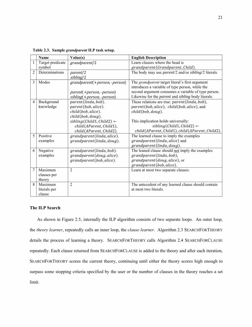
21

The ILP Search

As shown in Figure 2.5, internally the ILP algorithm consists of two separate loops. An outer loop,

the theory learner, repeatedly calls an inner loop, the clause learner. Algorithm 2.3 SEARCHFORTHEORY

details the process of learning a theory. SEARCHFORTHEORY calls Algorithm 2.4 SEARCHFORCLAUSE

repeatedly. Each clause returned from SEARCHFORCLAUSE is added to the theory and after each iteration,

SEARCHFORTHEORY scores the current theory, continuing until either the theory scores high enough to

surpass some stopping criteria specified by the user or the number of clauses in the theory reaches a set

limit.

Table 2.3. Sample grandparent ILP task setup.

Name Value(s) English Description

1 Target predicate

symbol grandparent/2 Learn clauses where the head is

( ).

2 Determinations parent/2 sibling/2

The body may use parent/2 and/or sibling/2 literals.

3 Modes grandparent(+person, -person) parent(+person, -person) sibling(+person, -person)

The grandparent target literal’s first argument

introduces a variable of type person, while the

second argument consumes a variable of type person.

Likewise for the parent and sibling body literals.

4 Background

knowledge

( ) ( ) ( )

( ).

( ).

( ).

( ).

( )

( ) ( )

These relations are true: ( ) ( ) ( ) and

( )

This implication holds universally:

5 Positive

examples ( ) ( )

The learned clause to imply the examples

( ) and

( ).

6 Negative

examples ( ) ( ).

( ).

The leaned clause should not imply the examples

( ) ( ) or

( ) 7 Maximum

clauses per

theory

2 Learn at most two separate clauses.

8 Maximum

literals per

clause

2 The antecedent of any learned clause should contain

at most two literals.

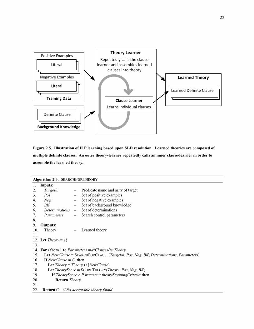
22

Algorithm 2.3. SEARCHFORTHEORY

1. Inputs:

2. Target/n – Predicate name and arity of target

3. Pos – Set of positive examples

4. Neg – Set of negative examples

5. BK – Set of background knowledge

6. Determinations – Set of determinations

7. Parameters – Search control parameters

8.

9. Outputs:

10. Theory – Learned theory

11.

12. Let Theory = {}

13.

14. For i from 1 to Parameters.maxClausesPerTheory

15. Let NewClause = SEARCHFORCLAUSE(Target/n, Pos, Neg, BK, Determinations, Parameters)

16. If NewClause ≠ then

17. Let Theory = Theory NewClause}

18. Let TheoryScore = SCORETHEORY(Theory, Pos, Neg, BK)

19. If TheoryScore > Parameters.theoryStoppingCriteria then

20. Return Theory

21.

22. Return // No acceptable theory found

23.

Theory Learner

Repeatedly calls the clause learner and assembles learned

clauses into theoryLogical SentenceLogical Sentence

Positive Examples

Literal

Training Data


Negative Examples

Literal

Logical SentenceLogical SentenceDefinite Clause


Learned Theory

Learned Definite ClauseLearned Definite ClauseLearned Definite Clause

Clause Learner

Learns individual clauses

Figure 2.5. Illustration of ILP learning based upon SLD resolution. Learned theories are composed of

multiple definite clauses. An outer theory-learner repeatedly calls an inner clause-learner in order to

assemble the learned theory.

23

Each invocation SEARCHFORCLAUSE searches for a single clause and returns the learned clause (if

any) to the theory learner. The clause learner performs the actual search of the hypothesis space for

clauses, using a standard best-first search. In the Aleph-style “top-down8” search, the clause learner

searches the hypothesis starting with the most-general clause (e.g.,

( ) from the sample task definition) and expands each node

according to the determinations and modes (discussed further below), generating candidate clauses. At

8 Aleph is top-down with respect to a lattice of possible clauses, where the top of the lattice is the most-general clause and the

bottom of the lattice is the most specific clause containing all possible literal extensions. Bottom-up approaches exists but are

not discussed here.

Algorithm 2.4. SEARCHFORCLAUSE

1. Inputs:

2. Target/n – Predicate name and arity of target

3. Pos – Set of positive examples

4. Neg – Set of negative examples

5. BK – Set of background knowledge

6. Determinations – Set of determinations

7. Parameters – Search parameters

8.

9. Output:

10. Clause – Learned clause

11.

12. Let RootClause = target(Arg1, …, ArgN) ← true.

13. Let RootScore = SCORECLAUSE(RootClause, Pos, Neg, BK)

14. Let Open = {<RootClause / RootScore>}

15.

16. While Open != do

17. Let ClauseToExpand = head of Open

18. For Predicate Determinations do

19. Let Extensions = EXTENDCLAUSE(ClauseToExpand, Predicate)

20. For NewClause Extensions

21. Let NewScore = SCORECLAUSE(NewClause, Pos, Neg, BK)

22. If NewScore > Parameters.clauseStoppingCriteria then

23. Return NewClause

24. else

25. Add <NewClause / NewScore> to Open in ascending order of score

26.

27. Return // No acceptable clause found

24

each step, the possible expansions are scored and the resulting score determines both the next expanded

node and controls when the clause search is stopped. Figure 2.6 depicts a simple clause search based upon

the sample task from Table 2.3.

Covers all positives and all negatives.Keep searching.

grandparent(Grandprt, Child) parent(Grandprt, Child)

Covers all positive and only two negatives.Keep searching.

grandparent(Grandprt, Child) parent(Grandprt, Parent)

grandparent(Grandprt, Child) parent(Grandprt, Parent), parent(Parent, Child)

Covers three positives and no negatives. Meets stopping criteria. Return clause.

Covers no positives and no negatives. Abandon branch.

grandparent(Grandprt, Child) true1

2

3

4

Figure 2.6. Illustration of an ILP search for a learned clause. The clause learner generates candidate

clauses, arranged in a tree structure, using the literals specified by the user. At each step, the clause is

scored against the positive and negative examples. The score determines when the search should stop as

well as controlling the order of the search. The numbers indicate the order in which the clause learner

searched the clauses.

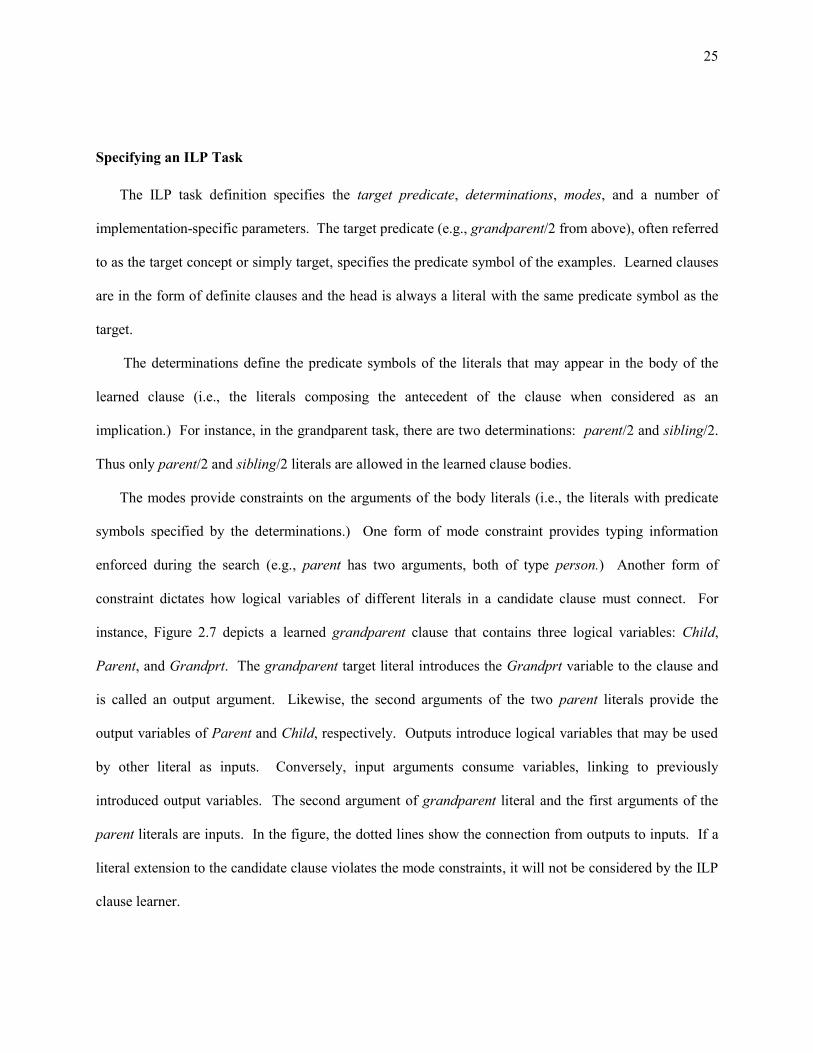
25

Specifying an ILP Task

The ILP task definition specifies the target predicate, determinations, modes, and a number of

implementation-specific parameters. The target predicate (e.g., grandparent/2 from above), often referred

to as the target concept or simply target, specifies the predicate symbol of the examples. Learned clauses

are in the form of definite clauses and the head is always a literal with the same predicate symbol as the

target.

The determinations define the predicate symbols of the literals that may appear in the body of the

learned clause (i.e., the literals composing the antecedent of the clause when considered as an

implication.) For instance, in the grandparent task, there are two determinations: parent/2 and sibling/2.

Thus only parent/2 and sibling/2 literals are allowed in the learned clause bodies.

The modes provide constraints on the arguments of the body literals (i.e., the literals with predicate

symbols specified by the determinations.) One form of mode constraint provides typing information

enforced during the search (e.g., parent has two arguments, both of type person.) Another form of

constraint dictates how logical variables of different literals in a candidate clause must connect. For

instance, Figure 2.7 depicts a learned grandparent clause that contains three logical variables: Child,

Parent, and Grandprt. The grandparent target literal introduces the Grandprt variable to the clause and

is called an output argument. Likewise, the second arguments of the two parent literals provide the

output variables of Parent and Child, respectively. Outputs introduce logical variables that may be used

by other literal as inputs. Conversely, input arguments consume variables, linking to previously

introduced output variables. The second argument of grandparent literal and the first arguments of the

parent literals are inputs. In the figure, the dotted lines show the connection from outputs to inputs. If a

literal extension to the candidate clause violates the mode constraints, it will not be considered by the ILP

clause learner.

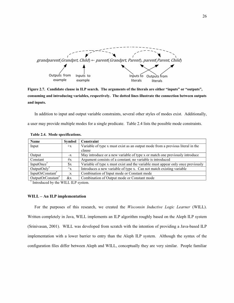
26

In addition to input and output variable constraints, several other styles of modes exist. Additionally,

a user may provide multiple modes for a single predicate. Table 2.4 lists the possible mode constraints.

WILL – An ILP implementation

For the purposes of this research, we created the Wisconsin Inductive Logic Learner (WILL).

Written completely in Java, WILL implements an ILP algorithm roughly based on the Aleph ILP system

(Srinivasan, 2001). WILL was developed from scratch with the intention of providing a Java-based ILP

implementation with a lower barrier to entry than the Aleph ILP system. Although the syntax of the

configuration files differ between Aleph and WILL, conceptually they are very similar. People familiar

Table 2.4. Mode specifications.

Name Symbol Constraint

Input +x Variable of type x must exist as an output mode from a previous literal in the

clause

Output -x May introduce or a new variable of type x or match one previously introduce

Constant #x Argument consists of a constant; no variable is introduced

InputOnce† $x Variable of type x must exist and the variable must appear only once previously

OutputOnly† ^x Introduces a new variable of type x. Can not match existing variable

InputOrConstant† :x Combination of Input mode or Constant mode

OutputOrConstant† &x Combination of Output mode or Constant mode

† Introduced by the WILL ILP system.

Figure 2.7. Candidate clause in ILP search. The arguments of the literals are either “inputs” or “outputs”,

consuming and introducing variables, respectively. The dotted lines illustrate the connection between outputs

and inputs.

grandparent(Grandprt, Child) parent(Grandprt, Parent), parent(Parent, Child)

Inputs toexample

Inputs toliterals

Outputs fromliterals

Outputs fromexample

27

with Aleph should be able to adapt to WILL. While written in Java, WILL provides Prolog-like9 logic

inference. We primarily designed WILL to facilitate research of ILP approaches as well as providing a

platform for other research using the ILP learning.

WILL implements several extensions to the Aleph algorithm. First, Aleph only supports a flat type

hierarchy in the type constraints specified by mode. WILL extends the Aleph system by supporting a

hierarchical typing scheme. This allows an is-a hierarchy (e.g., Figure 2.8) to be employed when defining

the search space. Hierarchical typing allows the user to better constrain the search space and has proven

useful in our research. The second major difference between Aleph and WILL is the addition of several

new modes. WILL support the additional modes constraints annotated by a dagger symbol (†) in Table

2.4. These additions allow the user to better control the construction of the search space.

9 WILL follows basic Prolog semantics with regards to inference rules and order. However, WILL supports only a subset of the

standard Prolog predicates and language structures.

vehicle

car truck bus

compact suv

Figure 2.8. An is-a hierarchy. The types of objects form a tree where sub-trees represent subtypes of the

parent type.

28

2.2.4 Support Vector Machines

Support Vector Machines (SVMs) (Cristianini & Shawe-Taylor, 2000) are a state-of-the-art method

for both classification and regression10 tasks. SVMs belong to a class of learning algorithms called

maximum-margin (or max-margin) algorithms. Maximum-margin algorithms attempt to learn models

that maximize the distance between the decision boundary and the training examples nearest to the

decision boundary, as shown in Figure 2.9. These examples nearest to the decision boundary, along with

misclassified examples, are called the support vectors. SVM have the property that only the support

vectors play a role in defining the decision boundary. For instance, in Figure 2.9 there are four examples

that are support vectors. If the training set consisted of only these examples, the learned model would be

the same as the model learned with the original training data. This property is where SVMs get their

name and provides the advantage that only the support vectors need to be retained after learning in order

to evaluate the model.

SVMs are based upon a linear mathematical model. However, in many tasks the positive and

negative training examples are not linearly separable. For instance, in Figure 2.10 (left), the positive and

negative examples cannot be separated by a linear boundary. However, under some transformation θ that

maps the original feature space into a new feature space, the examples may be separable, as shown in

Figure 2.10 (right). In an SVM, the transformation θ is provided by a kernel. In many task, kernels

greatly increase the effectiveness of SVMs.

10 When used for regression, the SVM algorithm is often called support vector regression (SVR).

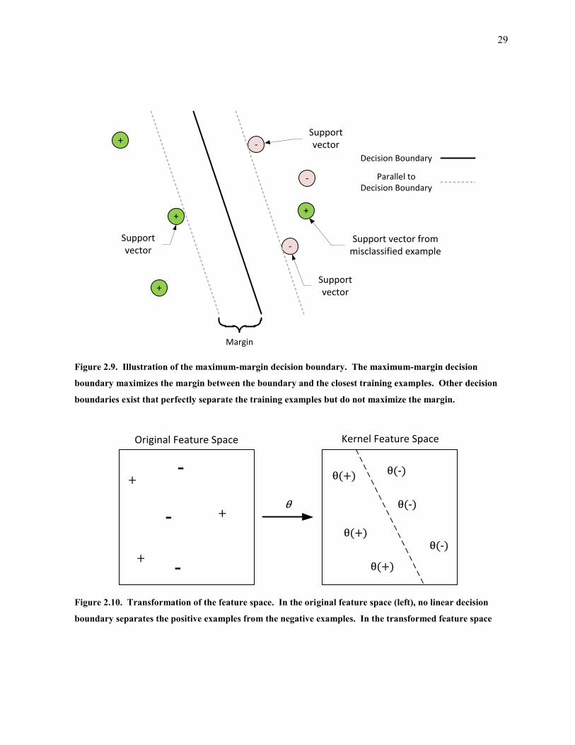
29

+

+

+-

-

- (+)

(-) (+)

(+)

(-)

(-)

Original Feature Space Kernel Feature Space

Figure 2.10. Transformation of the feature space. In the original feature space (left), no linear decision

boundary separates the positive examples from the negative examples. In the transformed feature space

(right), created by applying transformation θ, the examples are linearly separable.

+

+

-

-

+

-

Margin

Decision Boundary

Parallel toDecision Boundary

Support vector

Support vector

Support vector

+

Support vector from misclassified example

Figure 2.9. Illustration of the maximum-margin decision boundary. The maximum-margin decision

boundary maximizes the margin between the boundary and the closest training examples. Other decision

boundaries exist that perfectly separate the training examples but do not maximize the margin.

30

Typically SVMs formulate both classification and regression as either linear or quadratic-

programming optimization problems. While there are many different formulations for the SVM

optimization problem, all are conceptually similar. One formulation for SVM regression follows.

Let the training set consisting of m example feature vectors ∈ and the corresponding

regression target values ∈ . Let the ’s be the rows of the matrix ∈ and let ∈ be a

column vector of the ’s. An SVM learns a model of the form

( ) (2.4)

where vector w are the learned parameters11. The weight vector w can be replaced with its equivalent dual

form , which converts Equation (2.4) to

( ) (2.5)

where now represents the learned parameters. This is generalized, using the so-called “kernel trick”, by

replacing the term with ( ) to produce

( ) ( ) (2.6)

where ( ) is a kernel. A kernel is a positive definite function returning an inner product between its

arguments. In Equation (2.6), the kernel transforms the input feature space into a new feature space

called the kernel space. The discussion of kernels is beyond the score of this work. An excellent

discussion of them can be found in Cristianini & Shawe-Taylor (2000).

For any given , the error between ( ) and the target ’s over all training examples is

( ) ( ) (2.7)

or, by substituting Equation (2.6) for ( ),

( ) ( ) (2.8)

11 An offset b from the origin is typically included in this formulation. However, it can trivially be considered part of w and will

be ignored here.

31

From here, it is easy to formulate a linear that minimizes this error measure. Equation (2.9) provides

one simple linear program formulation.

( )‖ ‖ ‖ ‖

( )

(2.9)

In this formulation, the latent vector s measures the error of the solution on each training example and

penalizes inaccuracies via the objective function. Minimizing the 1-norm of s forces the error term

towards zero. Meanwhile, minimizing the 1-norm of penalizes solutions that are more complex in

order to avoid over fitting. The value is a fixed (though tunable) parameter that trades off the

accuracy of the solution on the training examples versus the complexity the solution. This linear program

can be solved using standard linear program optimization methods.

Other formulations exist that optimize a different error function, such as the squared error. These

formulation often result in quadratic programs, which can take more computation to solve, but may

produce better results. Furthermore, due to the simplicity of the linear or quadratic program, additional

constraints can be added to produce refined results. This is the approach taken by knowledge-based

support vector machines (KB-SVM) (Mangasarian, Shavlik, & Wild, 2004) to allow advice to be included

in addition with the training examples.

2.2.5 Boosted Relational Dependency Networks

Boosted relational dependency networks (bRDN) (Natarajan, Khot, Kersting, Gutmann, & Shavlik,

2010) provide a relational, probabilistic graphical-model classification algorithm. Probabilistic models

perform classification by estimating the probability of each predicted class given the description of an

example. Graphical models provide a method to factor a probabilistic model into a more manageable

form (Koller & Friedman, 2009). The details of probabilistic graphical models are beyond the scope of

this document and I will only describe boosted relational dependency networks that I use later.

32

A dependency network (Heckerman, Chickering, Meek, Rounthwaite, & Kadie., 2001) approximates

a joint distribution over the variables as product of conditional distributions. Relational dependency

networks (RDN) (Neville & Jensen, 2007) extend these dependency networks to a relational setting. The

bRDN algorithm combines relational dependency networks with a form of gradient-tree boosting

(Dietterich, Ashenfelter, & Bulatov, 2004), in order to improve the performance of the underlying RDN

approach.

RDNs consist of a set of predicate symbols composing the nodes of a graphical model. For each

predicate Yi, a conditional probability distribution P(Yi | Xi ), defines a distribution over the values of Yi

given the values of the other features. The distribution of a variable yi is estimated as

r ( ) e ( )

∑ e ( )

∀ ∈ ≠ (2.10)

Where ( ) is the potential function of yi given all other features ≠ .

The bRDN algorithm approximates these conditional probability distributions (the s) through

relational decision trees (Blockeel & De Raedt, 1998). A sample tree is depicted in Figure 2.11. Like

inductive logic programming techniques, bRDNs use relational background knowledge when learning a

tree. In these relational decision trees, each interior node is a logical decision point and the leaf nodes

represent the various potentials, i.e., the ’s, of the conditional probability distribution. In order to obtain

the final probabilities, the potentials must be normalized according to Equation (2.10).

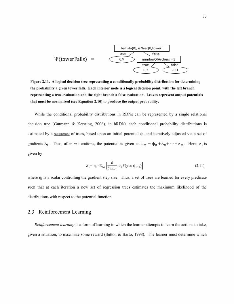
33

While the conditional probability distributions in RDNs can be represented by a single relational

decision tree (Gutmann & Kersting, 2006), in bRDNs each conditional probability distributions is

estimated by a sequence of trees, based upon an initial potential and iteratively adjusted via a set of

gradients . Thus, after m iterations, the potential is given as . Here, is

given by

[

( )] (2.11)

where is a scalar controlling the gradient step size. Thus, a set of trees are learned for every predicate

such that at each iteration a new set of regression trees estimates the maximum likelihood of the

distributions with respect to the potential function.

2.3 Reinforcement Learning

Reinforcement learning is a form of learning in which the learner attempts to learn the actions to take,

given a situation, to maximize some reward (Sutton & Barto, 1998). The learner must determine which

true false

ballista(B), isNear(B,tower)

true false

numberOfArchers > 5

-0.10.7

0.9 (towerFalls) =

Figure 2.11. A logical decision tree representing a conditionally probability distribution for determining

the probability a given tower falls. Each interior node is a logical decision point, with the left branch

representing a true evaluation and the right branch a false evaluation. Leaves represent output potentials

that must be normalized (see Equation 2.10) to produce the output probability.

34

sequence of actions results in the highest weighted sum of rewards12. An action may not result in an

immediate reward but may affect long-term rewards. Unlike supervised learning where the training data

is static, reinforcement learning usually13 requires the learner to act within the environment in order to

obtain training data. This leads to a situation in which early learning decisions can affect later learning

since different data will be available depending on the earlier choices by the learner.

2.3.1 Task Definition

A reinforcement-learning problem consists of an environment and an agent. The agent operates

within the environment according to some policy, a definition of what actions to take in a given state.

The agent-environment interaction is called a cycle, as shown in Figure 2.12. The learner controls the

agent as it interacts with the environment. At time t, the environment provides the agent information

about the current state of the world st. The agent then selects an action at from a set of legal actions. The

environment provides feedback to the learner in the form of a reward signal rt and updated agent state

information st+1 according to the outcome of the selected action. The reward is a real-valued number.

The state describes the agent’s situation within the environment and the state can be represented in a

variety of ways, such as a unique state identifier, a fixed-length feature vector, or a set of relational facts

describing the environment. The set of possible actions is typically discrete. The outcomes of the actions

may be deterministic or stochastic, depending upon the task definition.

The specification of an environment, along with the available actions, describes a single

reinforcement-learning task. Groups of related reinforcement-learning tasks, which share similar

12 Other target reward formulations, such as average reward, also exist. The weighted sum reward is arguably the most

commonly used. 13 If the learner is provided with a complete formal description of the environment, it can learn a policy without interacting with

the environment.

35

environments, belong to the same reinforcement-learning domain. Tasks in the same domain often share

the same underlying rules (i.e., “physics”) dictating the operation of the environments, but often differ in

action sets, state description, and reward function. For instance, within a soccer domain, there might exist

the two tasks of KeepAway and BreakAway (a game where keepers attempt to keep the ball away from

takers and a game where an offensive team attempts to score a goal against a defensive team,

respectively). Tasks that vary only by size or topology, such as 3-person KeepAway versus 5-person

KeepAway or two mazes with different layouts, are also separate tasks since their optimal solutions are

different.

A Markov Decision Process (MDP) formally describes a reinforcement-learning environment. An

MDP consists of a 5-tuple {S, A, P, R, } with a set S of states, a set A of actions, a probability

distribution P, a reward function R, and a discount factor ∈ ( . ∈ [ represents the

probability of transitioning from state s to state s’ via action a. ∈ represents the reward received

when action a is taken from state s. The set of possible states may be infinite, while the set of actions is

typically discrete.

Learner Environment

action

reward

state

Figure 2.12. Reinforcement-learning environment-agent interaction. An agent receives state information

from the environment. Based upon that information, the agent chooses an action to perform. The

environment determines the outcome of performing the indicated action and presents the agent with a

reward and updated state information.

36

A learner learns a policy : S A [0,1], representing the probability the agent will perform action

a A from state s S. The learner attempts to learn policies that maximize some measure of total

reward. The discounted total reward

0

t

total t

t

R r

(2.12)

is a common measure. If γ = 1, the discounted total reward is simply the total reward received, called the

Monte Carlo reward. An optimal policy * is a policy that results in the maximum achievable reward for

a given MDP.

Figure 2.13 illustrates the environment of a maze task and Table 2.5 provides a description of the

MDP parameter values. In the maze task, an agent must navigate through a maze to reach an exit. The

size and topology of a maze is fixed. Mazes with different sizes or topologies are considered different,

albeit related, reinforcement-learning tasks.

Agent

Exit

Figure 2.13. A sample maze reinforcement-learning task. The agent must discover a path through the

maze to the exit. A large positive reward is received when the exit is reached and a small negative reward

is received for each action taken.

37

The agent starts at a specific location and may attempt to move in each of the cardinal directions. A

move action results in the position of the agent moving one unit in the appropriate direction, unless a wall

blocks the agent, in which case the agent remains in the same state. A large positive reward (+10) is

received for reaching the exit and a small negative reward (-1) is received for each action that does not

result in reaching the exit.

The state representation for the maze task consists of six features: two integer features representing

the current x and y location of the agent and four Boolean features, wall(north), wall(south), wall(east),

and wall(west), indicating whether a wall is present immediately adjacent to the agent in the indicated

direction.

2.3.2 Optimal Policies and the Bellman Equations

Bellman (1957) performed some of the earliest research into reinforcement learning. He proposed a

method to calculate an optimal policy for a Markov decision process using a value function mapping

states to the reward. Bellman’s original function definition, now called the Bellman equation, provides

the basis for many reinforcement-learning approaches.

Many derivatives of the original Bellman equation exist. Equation (2.13) defines the value function

V*(s) for state s, which is the expect discounted reward received for always taking an optimal action from

the given state.

Table 2.5. MDP parameter values for sample Maze task.

MDP Parameter Values

S – States All locations in the maze. Features include x and y coordinates and the existence or

absence of walls in the cardinal directions.

A – Actions The agent can move in any of the four cardinal directions.

P – Probability of

next state

If no wall blocks the movement, the agent deterministically moves to the state a single

space in the direction of the selected action. Otherwise, agent remains in same state.

R – Reward +10 If goal state reached.

-1 otherwise.

γ 1

38

( )

∑ [

( )]

(2.13)

While value function from Equation (2.13) provides a way to calculate the expect reward for taking

the best action it does not specify which action is the optimal action. Another variation of the Bellman

equation, shown in Equation (2.14), provides the state-action function ( ), typically called the Q-

function, which allows the optimal action to be determined. Given the optimal Q-function, the optimal

action for a state s is r ( ).

( ) ∑ [

( )]

(2.14)

Both of these equations require knowledge of all the MDP parameters. While early research in

reinforcement learning focused on computational techniques necessary to apply the Bellman equations,

later research examined how to perform reinforcement learning without a full definition of the MDP.

2.3.3 Common Reinforcement Learning Approaches

Many different reinforcement-learning algorithms exist. The approaches can be roughly categorized

according to what MDP parameters are known as well as how the algorithm approaches finding the

optimal policy. Figure 2.14 provides a brief taxonomy of some of the different RL scenarios and

approaches.

In some cases, all MDP values are known, including the state-transition function and the reward

function (left most branch of figure). When the complete MDP definition is known, finding the optimal

policy is strictly a computational task, requiring no interaction with the environment. There are several

approaches to computing the policy in this scenario, based on the Bellman equations. For instance, when

the MDP state set is discrete, the optimal policy can be calculated using dynamic programming. In cases

of infinite state sets, approaches exist that calculate the policy by iteratively applying the Bellman

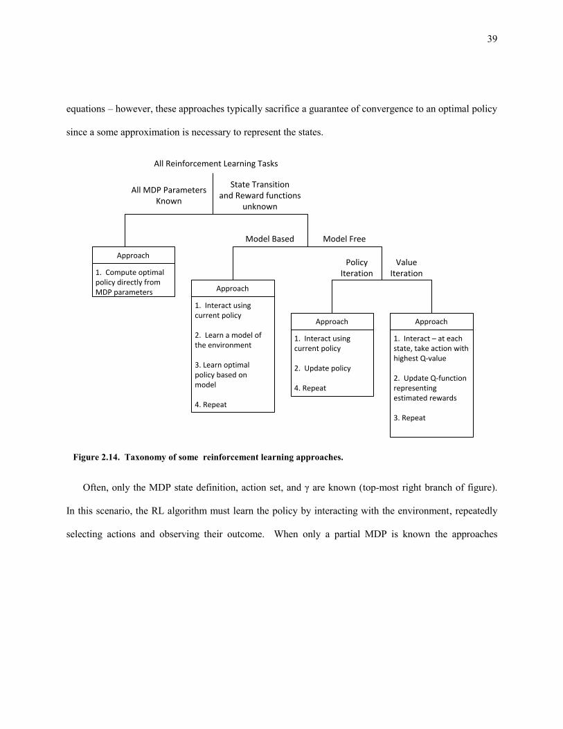
39

equations – however, these approaches typically sacrifice a guarantee of convergence to an optimal policy

since a some approximation is necessary to represent the states.

Often, only the MDP state definition, action set, and γ are known (top-most right branch of figure).

In this scenario, the RL algorithm must learn the policy by interacting with the environment, repeatedly

selecting actions and observing their outcome. When only a partial MDP is known the approaches

All Reinforcement Learning Tasks

All MDP Parameters Known

State Transition and Reward functions

unknown

1. Compute optimal policy directly from MDP parameters

Model Based Model Free

1. Interact using current policy

2. Learn a model of the environment

3. Learn optimal policy based on model

4. Repeat

Approach

Approach

1. Interact using current policy

2. Update policy

4. Repeat

Approach

1. Interact – at each state, take action with highest Q-value

2. Update Q-function representing estimated rewards

3. Repeat

Approach

Policy Iteration

Value Iteration

Figure 2.14. Taxonomy of some reinforcement learning approaches.

40

generally fall into two classes: model-based and model-free. Model-free approaches can further be

divided into value-iteration and policy-iteration14.

Model-Based Reinforcement Learning

Model-based approaches constitute one major classes of algorithms used to solve RL tasks15. While

model-based approaches consist of a diverse class of algorithms, all model-based approaches have a

common feature; they attempt to learn a model of the underlying task, iteratively updating that model

while interacting with the environment. The algorithm then determines the policy to follow based upon

the learned model.

Depending on the approach, the learned models vary greatly in both form and level of detail. Some

model-based approaches attempt to build a complete predictive model of the environment, effectively

attempting to model the state-transition and reward functions of the underlying MDP (Sutton, 1991).

Other approaches attempt to create an abstraction of the underlying MDP, maintaining some congruency

to the original, but abstracting aspects that are either difficult to learn or irrelevant to producing a usable

policy (Kersting, Van Otterlo, & De Raedt, 2004; Morales, 2003; Van Otterlo, 2003). Still others model

only limited aspects of the MDP, such as transition probabilities or reward functions (Croonenborghs,

Ramon, Blockeel, & Bruynooghe, 2006; Pasula, Zettlemoyer, & Kaelbling, 2004).

Model-Free Value-Iteration Reinforcement Learning

Model-free value-iteration is a class of reinforcement-learning algorithms that estimate a state-action

value function without learning an underlying model. The state-action value function is called the Q-

function and the class of algorithms that learn the Q-function is referred to as Q-learning (Watkins &

14 Value-iteration and policy-iteration approaches exist for all branches of the provided taxonomy but are beyond the scope of

this document. 15 The term model-based is sometimes used to refer to approaches where the complete MDP definition is known. However, in

recent literature, this usage is less common.

41

Dayan, 1992). The state-action value function maps state-action pairs to real-values

representing the expected reward that will be received by taking an action from a state. The policy π

followed by the learner depends upon the Q-function; at each time step, the learner takes the action with

the highest Q-value. Additionally, the learner typically takes random exploratory action with some small

probability.

Figure 2.15 depicts a Q-function for the maze task defined in Table 2.5. In the figure, the numeric

values represent the expected reward (i.e., the Q-value) for taking each of the indicated movement

directions.

The learning algorithm estimates the Q-function over time by iteratively updating the Q-function. As

the learner interacts with the environment, the learner adjusts its current Q-function according to the

formula

83

8

9

8

7

4

3

3

2

5

4

3

4

5

6

4

5

7 7

6

5

7

6

6

3 2

2

4

5

6

5

2

3

2

4

3

3

5

4

2

2

3

2

3

3

4

3

7

8

9

8

6

7

8

7

6

6

7

5

Figure 2.15. Example of the Q-function for a maze task. For each state in the maze, each action has an

associated Q-value, representing the expected non-discounted reward received for taking that action (and

following the policy afterwards). The Q-values shown are the reward values after the Q-function has

converged to the optimal values.

42

1'

'( , ) (1 ) ( , ) max ( , ')t t t t t ta

Q s a Q s a R Q s a (2.15)

where, at each time step t, st denotes the state, the at denotes the action taken, rt denotes the reward

received, and st+1 denotes the resulting new state. This formula, based upon the Bellman equations,

estimates a new Q-value '( , )t tQ s a for a state and action by combining the previous estimated value

( , )t tQ s a with a new estimate based upon the observed information1

'max ( , ')t t

aR Q s a . Here,

(0 1) controls the learning rate of the algorithm. Over time decreases so that later interactions

have smaller impact on the learned model.

Under certain conditions, the policy resulting from repeatedly interacting with the environment and

updating the Q-function converges to an optimal policy (Watkins & Dayan, 1992). This, for instance,

occurs in discrete domains when every state-action Q-value is stored separately in a Q-table (a table with

a value for every possible state-action combination), every state-action pair is visited infinitely often, and

the learning rate decreases appropriately over time. Even when these assumptions are violated, Q-

learning often results in a high-quality policy that performs well empirically, but may not be optimal

(Sutton & Barto, 1998).

In practice, many of the tasks in which we are interested are continuous or are discrete, but the state

and action space is so large it becomes infeasible to store the Q-values in a table. In these cases, Q-

learner approaches use a regression-function, supervised learner (usually called a function approximator)

to estimate the Q-function. The use of a function approximator usually violates the assumption necessary

for guaranteed convergence, but has the advantage of allowing the learner to generalize the Q-function

with respect to the state space. This generalization often increases the learning rate by reducing the

number of states the learner must visit.

Numerous refinements to the basic Q-learning algorithm exist. These include temporal-difference

methods (Sutton, 1988) that provide better convergence properties; SARSA approaches (Rummery &

43

Niranjan, 1994) designed to more accurately model the current policy; and relational extensions that

allow complex relational domains to be handled more naturally (Džeroski, De Raedt, & Blockeel, 1998).

Model-Free Policy-Iteration Reinforcement Learning

Policy iteration provides a second class of algorithms used in model-free reinforcement learning16.

Policy iteration methods forego maintaining a Q-function, instead representing the policy : S A

[0,1] explicitly. The class of policy-iteration approaches is more diverse than value-iteration approaches.

In value iteration, the Bellman equations define how interaction with the environment changes the

policy. Although some policy iteration approaches use the Bellman equations, not all do. In the absence

of a Q-function, policy iteration requires different policy-refinement method. For instance, Whitley et. al.

(1993) use genetic algorithms to find a policy by randomly mutating the current policy multiple times,

selecting the best new policy, and mutating it again. At no point does the algorithm attempt to estimate

the expected reward as value-iteration approaches would. Policy iteration is not used in this research and

further details are beyond the scope of this document.

16 Policy iteration has several meanings, depending on the source. Sutton and Barto (1998) present a specific algorithm which

they call policy iteration. Here I present a wider view of policy iteration not tied to that specific implementation.

44

3 Testbeds

In order to evaluate the work presented here, I use a number of different evaluation tasks. Bootstrap

learning is a set of third-party tasks used to evaluate the advice-taking contributions in Chapter 4.

Wargus is an open-source real-time strategy video game used to evaluate the advice-giving human-

computer interface work in Chapter 5. Chapter 6 uses several ILP tasks from the literature to evaluate

automated parameter tuning approaches. RoboCup is a soccer simulation used to evaluate the relational

reinforcement learning approaches in Chapters 7 and 8.

3.1 Bootstrap Learning ILP Tasks

The Bootstrap Learning (BL) project, funded by the United States Defense Advanced Research

Projects Agency (DARPA), explores a new learning paradigm proposed by Oblinger (2006) which views

machine learning as human-guided knowledge acquisition. In the BL setting, the machine learner induces

concepts that build upon one another through a “ladder” of tasks, which are organized as self-contained

lessons; lower rungs of the lesson ladder teach simpler concepts, which are learned first and then used to

learn − i.e., bootstrap − more complex concepts. The lessons in the project incorporate a wide variety of

natural teacher instruction methods, including providing domain descriptions, pedagogical examples,

telling of general instructions, demonstration, and feedback. Our role in the project involved learning

lesson using ILP taught through teacher provided examples and advice. These lessons are referred to as

by-example lessons.

The BL project consists of three independent domains: Unmanned Arial Vehicle (UAV), Armored

Task Force (ATF), and International Space Station (ISS). An independent third party developed all three

domains and each domain consists of a complete ladder of bootstrapped lessons. The domains are

described below.

45

Each lesson consists of a sequence of messages from the teacher to the learner. Teacher instruction

includes training examples and experts’ advice rules for certain examples, called the relevance

information, to help the student learn these tasks effectively. The messages that make up each lesson i.e.,

the teacher instructions to the student, are given using a general-purpose, strongly typed, object-oriented

language called Interlingua that was also developed under DARPA’s guidance by another third party for

the purposes of the BL project. For each lesson, we converted the messages into ILP facts and examples

expressed in first-order logic, specifically as Horn clauses.

Only a subset of the BL lessons are by-example lesson. In this document, I specifically look at 14 of

the by-example lessons, seven AFT lessons and seven UAV lessons. Table 3.1 summarizes the size of

the tasks in terms of the number of ground background knowledge facts of the tasks. Each of these

ground facts corresponds to a property of an object. For instance, in the UAV domain, the ground facts

include the location of the UAVs and information about the environment observable to a UAV such as the

location of near-by vehicles.

Table 3.1. Number of facts per lesson. This table lists the number of ground facts that have ILP modes,

broken down by both domain and task.

ATF Tasks # of Facts UAV Tasks # of Facts

CallsForColumnFormation 277,800 AssessGoal 193,400

CallsForEchelonLFormation 277,800 FullFuelTank 192,400

CallsForEchelonRFormation 277,800 IsASingleMovingTruck 197,313

CallsForLineFormation 277,800 IsASingleStoppedTruck 197,387

CallsForVeeFormation 277,800 Near 193,387

CallsForWedgeFormation 277,800 ReadyToFly 193,200

CompanyHasMinePlow 306,391 TruckIsAtIntersection 221,424

Average # of Facts

240,122

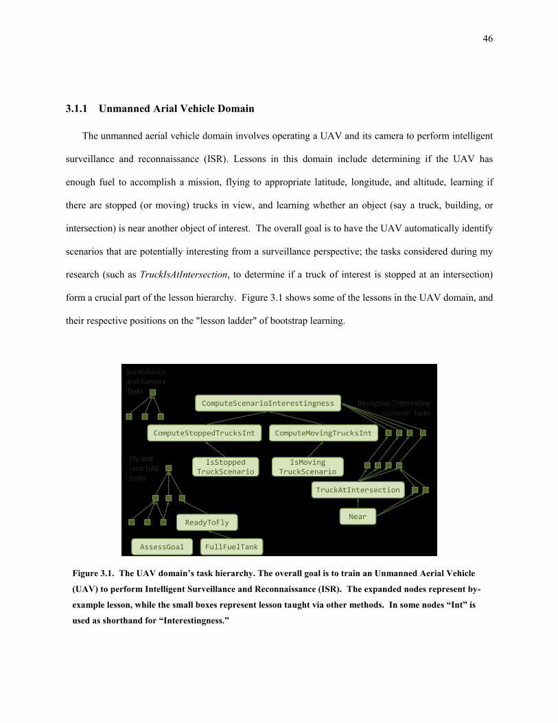
46

3.1.1 Unmanned Arial Vehicle Domain

The unmanned aerial vehicle domain involves operating a UAV and its camera to perform intelligent

surveillance and reconnaissance (ISR). Lessons in this domain include determining if the UAV has

enough fuel to accomplish a mission, flying to appropriate latitude, longitude, and altitude, learning if

there are stopped (or moving) trucks in view, and learning whether an object (say a truck, building, or

intersection) is near another object of interest. The overall goal is to have the UAV automatically identify

scenarios that are potentially interesting from a surveillance perspective; the tasks considered during my

research (such as TruckIsAtIntersection, to determine if a truck of interest is stopped at an intersection)

form a crucial part of the lesson hierarchy. Figure 3.1 shows some of the lessons in the UAV domain, and

their respective positions on the "lesson ladder" of bootstrap learning.

Figure 3.1. The UAV domain’s task hierarchy. The overall goal is to train an Unmanned Aerial Vehicle

(UAV) to perform Intelligent Surveillance and Reconnaissance (ISR). The expanded nodes represent by-

example lesson, while the small boxes represent lesson taught via other methods. In some nodes “Int” is

used as shorthand for “Interestingness.”

47

3.1.2 The Armored Task Force Domain

The goal of the ATF domain is to teach the learner how to command a company of armored platoons

moving from one battlefield location to another in accordance with military doctrine. These lessons are

also organized based on the complexity of tasks, following the bootstrap principle. At the lowest level are

the tasks concerning individual armored vehicles, terrain segments and enemy unit information. At a

higher level are tasks concerning platoons (sets of armored vehicles), while at the top-most level are the

tasks concerning the command of a company, which is a set of platoons.

3.2 Wargus Real-Time Strategy Tasks

In Chapter 5, I present a human-computer interface (HCI) approach to knowledge acquisition. I

utilize the Wargus (2002) video game to illustrate advice acquisition via the HCI. In Wargus, a real-time

strategy game, two or more players direct units such as peasants, swordsmen, archers, etc. in an attempt to

conquer opposing players. Play involves constructing buildings, producing unit, harvesting resources,

and directing attacks against opponents.

The complete Wargus game is more complex than necessary for my experiments. Instead, I use a

small subset of Wargus called tower defense. In tower defense, an attacking team consisting of a small

number of peasants, archers, swordsmen, and ballista attack a single tower belonging to the defenders.

The learning task consists of predicting whether the tower will survive the attack, given the number of

attacking and type of attacking units. Figure 3.2 depicts a typically tower defense game board.

Variations of the game board include the existence of moat and rivers and the number and type of the

attacking units.

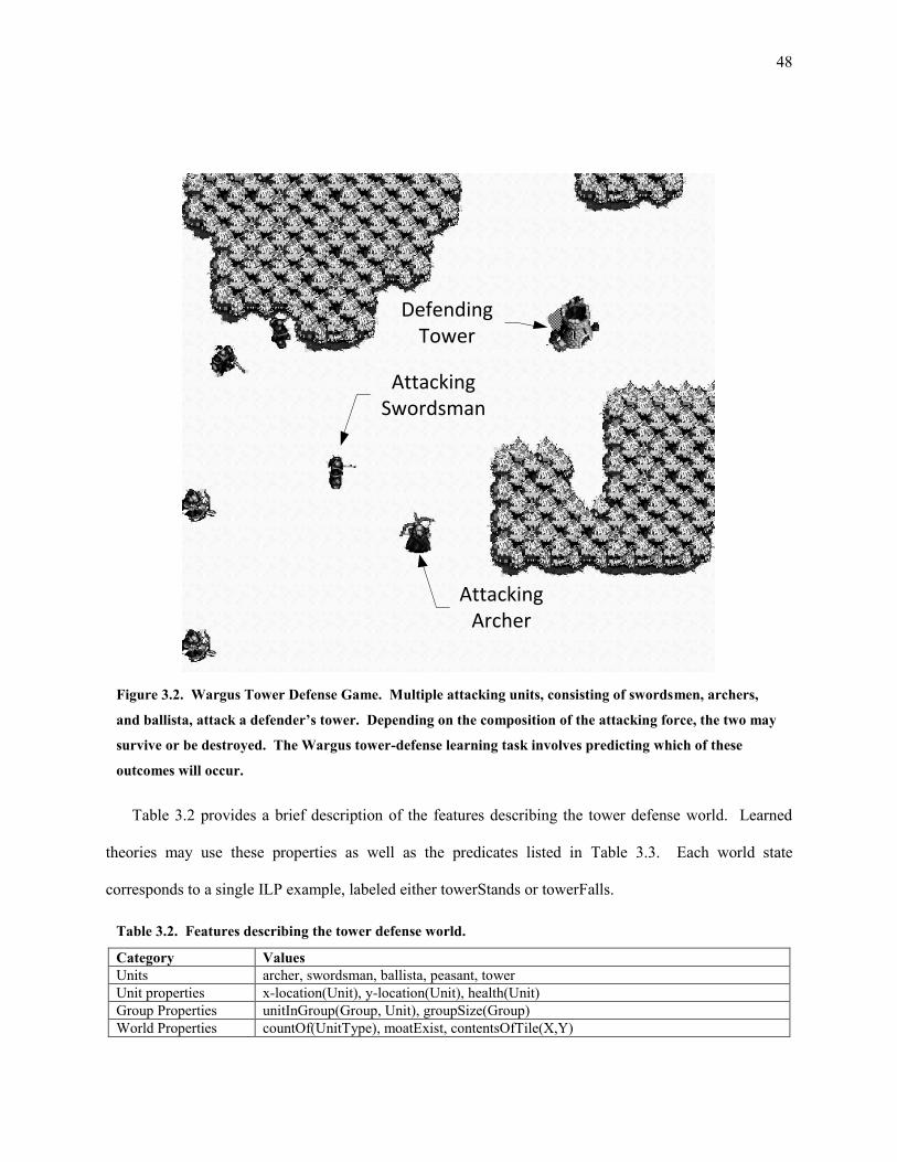
48

Table 3.2 provides a brief description of the features describing the tower defense world. Learned

theories may use these properties as well as the predicates listed in Table 3.3. Each world state

corresponds to a single ILP example, labeled either towerStands or towerFalls.

Table 3.2. Features describing the tower defense world.

Category Values

Units archer, swordsman, ballista, peasant, tower

Unit properties x-location(Unit), y-location(Unit), health(Unit)

Group Properties unitInGroup(Group, Unit), groupSize(Group)

World Properties countOf(UnitType), moatExist, contentsOfTile(X,Y)

DefendingTower

AttackingArcher

AttackingSwordsman

Figure 3.2. Wargus Tower Defense Game. Multiple attacking units, consisting of swordsmen, archers,

and ballista, attack a defender’s tower. Depending on the composition of the attacking force, the two may

survive or be destroyed. The Wargus tower-defense learning task involves predicting which of these

outcomes will occur.

49

3.3 Standard ILP Tasks

Chapter 6 uses several standard ILP tasks to evaluate automated parameter tuning approaches. These

tasks – advised-by, carcinogenesis, and mutagenesis – are detailed below.

3.3.1 Advised-By ILP Task

Introduced by Richardson and Domingos (2006), the advised-by ILP task involves learning rules

predicting if a professor advised a student, based upon a database describing the Department of Computer

Science and Engineering at the University of Washington (UW-CSE). The task includes 115 positive

examples and 1675 negative examples. Table 3.4 lists the predicates along with the total number of facts

defined in the task. All advised-by information consists of ground facts with no additional background

knowledge provided.

3.3.2 Carcinogenesis ILP Task

The carcinogenesis task, first used as an ILP testbed by Srinivasan et. al. (1997), involves learning

rules predicting carcinogenicity for a set of drugs. This task is considered an extremely challenging task,

Table 3.4. Advised-by ground facts (over all examples).

Predicate and Argument Types # of Facts

professor(person) 62

student(person) 216

yearsInProgram(person, years) 140

courseLevel(course, level) 132

taughtBy(course, person, quarter) 286

teachingAssistant(course, person, quarter) 481

inPhase(person, phase) 140

hasPosition(person, position) 52

Table 3.3. Predicates available for the “theories tower will stand” predication task.

Category Predicates

Numeric Comparitors greaterThan, lessThan, greaterThanOrEquals, lessThanOrEquals, equals

Spacial Comparitors isNearTo, isFarFrom, canReach

50

partially due to the large search space resulting from the extensive background knowledge. The task

includes 182 positive examples and 148 negative examples. Table 3.5 details the ground facts defined for

the carcinogenesis task. In addition to these ground facts, the task defines an extensive set of background

knowledge – listed in Table 3.6 – providing knowledge about the structure and chemical properties of the

various drugs. Although it is unnecessary to calculate all possible groundings of the background

knowledge, if generated, the number of grounding would exceed 100,000 additional facts.

3.3.3 Mutagenesis ILP Task

The mutagenesis task involves learning rules predicting the mutagenesis effect of certain drugs (e.g.,

drugs that changes the genetic material, usually DNA, of an organism and thus increases the frequency of

mutations above the natural background level.) With only 13 positive examples and 29 negative

examples, the mutagenesis proves difficult due to the low example counts. The ground facts, shown in

Table 3.6. Carcinogenesis background knowledge.

Background Knowledge Predicate and Argument Types

nitro(drug, ring) alkyl_halide(drug, ring)

sulfo(drug, ring) imine(drug, ring)

methyl(drug, ring) deoxy_amide(drug, ring)

connected(ring, ring) amide(drug, ring)

five_ring(drug, ring) ester(drug, ring)

non_ar_hetero_5_ring(drug, ring) carboxylic_acid(drug, ring)

non_ar_5c_ring(drug, ring) phenol(drug, ring)

hetero_ar_5_ring(drug, ring) alcohol(drug, ring)

carbon_5_ar_ring(drug, ring) sulfide(drug, ring)

six_ring(drug, ring) ether(drug, ring)

non_ar_hetero_6_ring(drug, ring) ketone(drug, ring)

non_ar_6c_ring(drug, ring) aldehyde(drug, ring)

hetero_ar_6_ring(drug, ring) amine(drug, ring)

benzene(drug, ring) methoxy(drug ring)

ar_halide(drug, ring)

Table 3.5. Carcinogenisis ground facts (over all examples).


alerts(drug, alerts, numberOfAlerts) 1143

atom(drug, atomid, element, integer, charge) 18506

has_property(drug, property, propertyValue) 1654

51

Table 3.7, define the basic atoms and chemical bond for the drugs occurring in the positive and negative

examples, as well as several other chemical properties. Additional background knowledge, shown in

Table 3.8, defines several additional chemical properties.

3.4 RoboCup Simulated Soccer Reinforcement Learning Domain

Chapter 7 and 8 present applications of ILP in reinforcement learning, using a set of tasks based upon

RoboCup (Kitano, 1997), a complex two-dimensional soccer simulation, originally intended for research

into robotics. To provide realism, the simulator is both stochastic and provides only noisy information to

the agents acting within the environment (i.e., the soccer players.) For these reasons, RoboCup is a

challenging testbed for reinforcement learning (Stone & Sutton, 2001) and the complete game is still

unsolved by state-of-the-art reinforcement-learning techniques.

Since the complete RoboCup soccer game is too complex to solve with current RL methods, several

RoboCup sub-tasks have been proposed by various researchers (see Figure 3.3). The first task within the

RoboCup domain, proposed by Stone and Sutton (2001), is M-on-N KeepAway. In this task, the

objective of the M players, called keepers, is to keep the ball away from N hand-coded players, called

Table 3.8. Mutagenesis background knowledge.

Background Knowledge Predicate and Argument Types

benzene(drug, ring)

carbon_5_aromatic_ring(drug, ring)

nitro(drug, ring)

methyl(drug, ring)

anthracene(drug, ringlist)

phenanthrene(drug, ringlist)

ball3(drug, ringlist)

Table 3.7. Mutagenesis ground facts (over all examples).


atom(drug, atomid, element, integer, charge) 5894

bond(drug, atomid, atomid, integer) 1654

lumo(drug, energy) 230

logp(drug, hydrophob) 230

52

takers. In KeepAway, the learner controls one of the keeper currently in possession the ball (the ball

holder), who has the action choices of holding the ball or passing it to one of the other keepers. All

players not in possession of the ball, including both keepers and takers, follow a hand-coded policy. The

learners receive a +1 reward for each time step their team keeps the ball; the game ends when the ball

either goes out of bounds or is intercepted by a taker. Stone and Sutton argue that effective KeepAway is

not only a challenging RL task by itself, but is also a significant step toward playing soccer.

Through the course of our research, we have developed several additional tasks beyond KeepAway.

Mobile KeepAway (Torrey, Shavlik, Walker, & Maclin, 2006) is an extension to KeepAway designed to

provide actions that are more interesting for the learner to utilize. Mobile KeepAway replaces the hold

ball action of KeepAway with four movement actions, move forward, move back, move left, and move

3-on-2

KeepAway

3-on-3

MoveDownfield

3-on-2

BreakAway

Figure 3.3. RoboCup soccer tasks. Several reinforcement learning task have been designed for the

RoboCup soccer simulator. Three such tasks are shown here.

53

right. Other aspects of the game remain the same as KeepAway. This game provides a richer selection of

actions from which knowledge can be extracted, which is important in our approaches.

M-on-N BreakAway (Torrey, Walker, Shavlik, & Maclin, 2005) is a task where the objective of the M

players called attackers is to score a goal against N-1 hand-coded defenders and a hand-coded goalie.

The game lasts until the attackers lose the ball, the attackers score a goal, the attackers kick the ball out of

bounds, or a play time exceeds 10 seconds. The learners receive a +1 reward for a goal and 0 reward

otherwise. The attacker who has the ball is controller by the learner and may choose to move (ahead,

away, left, or right with respect to the goal), pass to a teammate, or shoot at an area of the goal (either left,

right, or center). This task is particularly challenging to learn due to the sparse rewards received while

playing17.

M-on-N MoveDownfield (Torrey, Shavlik, Walker, & Maclin, 2006) is a task where the objective of

the attackers is to move toward the opposing team’s goal while maintaining possession of the ball. The

game ends when the attackers successfully move the ball past a certain position of the field, when an

opponent takes the ball, when the ball goes out of bounds, or after a time limit of 25 seconds. The

learners receive symmetrical positive and negative rewards for movement toward and away from the goal

line, respectively (i.e., for every “meter” of movement toward the goal, the learner received a +1 reward,

and for every “meter” of movement away from the goal, the learned received a -1 reward.) As with the

other tasks, attackers without the ball and the defenders follow a hand-coded strategy to receive passes.

The action set is the same as in BreakAway, except without the shoot actions.

The state representations for all four tasks are based upon the original representation developed by

Stone and Sutton (2001). Table 3.9 shows the predicates used in the relational features sets. Each

17 Often in reinforcement learning, a richer reward structure is use in order to facilitate learning. We intentionally used a sparse

reward in order to focus on the role of advice and knowledge transfer.

54

predicate represents one or more actual features, depending on the logical variables in the predicate and

the game size. For each state description, the player names (e.g., a0… aM for the attackers) are assigned

to the players according to their distance to the ball holder. Thus, a0 represents the attacker with the ball

(or k0 for KeepAway) and a1 is the keeper currently closest to a0. Empirically, Stone and Sutton found

that this ordering reduces the difficulty of the tasks.

Table 3.9. RoboCup task features. Arguments with capitol letters are logical variables. A complete list of

task features is generated by replacing variables with all appropriate constants. The ClosestTaker refers

to the taker closest to the keeper currently holding the ball. Likewise, the ClosestDefender refers to the

defender closest to the attacker currently holding the ball.

KeekAway and Mobile

KeepAway features

BreakAway and

MoveDownfield features

distBetween(k0, Player) distBetween(a0, Player)

distBetween(Keeper, ClosestTaker) distBetween(Attacker, ClosestDefender)

angleDefinedBy(Keeper, k0, ClosestTaker) angleDefinedBy(Attacker, k0, ClosestDefender)

xPosition(Object) xPosition(Object)

yPosition(Object) yPosition(Object)

distBetween(Keeper, fieldCenter) distBetween(Attacker, goalCenter)

distBetween(a0, GoalPart)

angleDefinedBy(GoalPart, a0, goalie)

angleDefinedBy(topRight, goalCenter, a0)

distBetween(Attacker, goalie)

angleDefinedBy(Attacker, a0, goalie)

timeLeft

55

4 Generation of Background Knowledge from

Advice about Specific Examples

Inductive Logic Programming (ILP) provides an effect method to learn logical theories in relational

domains. However, compared to most non-relational supervised learning algorithms, ILP requires a lot of

expert knowledge to setup a learning task. In addition to the standard supervised-learning information,

such as the positively labeled examples, the negatively labeled examples, and the known facts (i.e., the

example features), ILP often requires the user to define a complex corpus of background knowledge and

always requires the user to provide a specification of the search space. The ILP-setup problem of

articulating background knowledge can be difficult and requires detailed understanding of the ILP

algorithm, greatly limiting ILP’s usability by non-experts.

At least two possible solutions to this problem exist. One approach is to create a domain specific ILP

system. In this approach, first an ILP expert works closely with a domain expert to tailor the general-

purpose ILP algorithm to a specific domain, such as drug design (Finn, Muggleton, Page, & Srinivasan,

1998). Once the domain specific system has been created, domain experts, who are not ILP experts, can

then use the tailored system without in-depth ILP knowledge. While effective, this custom-system

approach does not fulfill our goal of increasing the usability of ILP without an ILP expert’s assistance. It

changes the point at which an ILP expert’s knowledge is required, but does not alleviate the expert’s

involvement.

56

A second solution to this ILP-setup problem, which retains the general-purpose nature of the ILP

system and alleviates the need of any ILP-expert assistance, is to allow a teacher18 to, as naturally as

technically possibly, explain why specific examples are positive or negative through some advice

language. This teacher-provided advice supplies hints about the concept being learned, beyond the

traditional labeling of examples. Given this teacher-provided advice, the automated learner can generate

background knowledge and setup the search space appropriately. In this chapter I present work exploring

this second approach. This is the first study to explore this approach, although some prior ILP work is

related and reviewed in Section 4.3. Much of the work presented in this chapter was performed in

collaboration with several others and presented in (Walker, et al., 2010).

Consider the following sample dialog between the teacher and the learner. Assume the formula

( ( ) ( )) ( ) is a relevant piece of background knowledge for concept C. The teacher

might express this indirectly via the following dialogue about a small number of training examples:

“In example 1, object a is a positive instance of concept C because ( ) is true.”

Note that, in human instruction, the teacher might say this to mean simply that p is relevant to C

rather than the complete definition of C.

“In example 2, object b is a positive instance of C because ( ) is true.”

Note here that an algorithm that induces background knowledge from these statements needs to

generalize both objects a and b to the same variable.

“In example 3, object d is a negative instance of C because ( ) is false.”

18 Throughout this chapter, I refer to the advice giver as the teacher. The teacher is typically a domain expert in the subject area

of the task, but who has not ILP expertise.

57

Note that the teacher is telling the learner about relevant background knowledge through a negative

example. The piece of advice in this case needs to be negated. In addition, the machine learner does

not know whether the advice is about (1) all possible choices for the second (or first) argument of q,

(2) restricting the choice of the second argument to be the same as the first, or (3) just the specific

choice of constant d as the second (or first) argument.

Although ( ( ) ( ) ) ( ) may be the formula necessary to define the concept, formulas

such as ( ( ) ( ) ) ( ), or ( ) ( ) ( ), or ( ) ( ( ) ( ) ), or

yet still others, are also consistent with this human-provided advice.

An additional benefit to allowing the teacher to provide such advice permits the use of ILP in an

setting in which only a few examples, along with teacher-provided annotations, are sufficient to learn the

target concept. In a setting with few examples, while the target concept might be complex, such as

( ( ) ( ) ) ( ), a simple clause, say ( ), by itself might be sufficient to discriminate

between examples. Thus, in this setting the advice should motivate the learner to prefer formulas that use

all the teacher-mentioned predicates (i.e., p, q and r), rather than just the simplest formula consistent with

the labeled examples.

Below, we present an algorithm to convert teacher-provided advice into ILP background knowledge.

We designed this algorithm with the sparse example setting in mind. Motivations for the algorithm we

present include the following:

1. High accuracy of the learned concept definition on teacher-labeled training examples.

2. Robustness in the presence of a small number of training examples and perhaps a total lack of

negative examples.

3. Inclusion of most, if not all, teacher-mentioned predicates in the learned concept definition.

4. Flexible combination and generalization of the teacher’s advice within and across examples.

5. Robustness to teacher errors, both in data labeling and advice.

58

6. Learned concepts may need to include predicates not mentioned in teacher-provided advice but

supplied as part of example descriptions.

Our primary motivation is to allow human users of ILP systems to express their knowledge about the

learning task at hand in whatever means seems most natural to them, from explaining (partially or fully)

why some specific examples are positive or negative members of the concept being learned, to simply

stating the proper categories (i.e., positive or negative) for other examples.

We present our approach as a “batch” system that is given a set of labeled examples and possibly

some advice about the examples, and then produces a set of one or more logical clauses (“inference

rules”) that best capture the concept being taught. However, we envision our approach as being best

situated in a setting where the human-machine dialog is continual; the human teacher provides some

initial training, the algorithm then learns, after which the teacher can provide additional guidance and the

process repeats until an acceptable concept description results (where ‘acceptable’ can either be based on

inspection of the learned clauses, or, more likely, on the quality of the predictions of the learned clauses

for new examples).

As mentioned above, we address the problem of effectively incorporating, into the ILP framework,

teacher-provided advice; a human teacher usually provides the latter and this interaction can be viewed

from the wider perspective of human-machine interaction. Such teaching refers to humans teaching

computers concepts and/or behaviors, through as natural and human-like dialog as possible. In our

setting, the taught concepts take the form of logical theories and the teacher provides relevance advice

about specific examples. The relevance advice takes a number of different forms, from simple “this

feature is important” advice to complex statements that can be mapped to a grounded form of the concept

being taught. The advice can be provided by a human familiar with the advice language but with no ILP

experience, i.e., a non-expert.

59

Figure 4.1 illustrates, using propositional logic for simplicity, how advice-generated background

knowledge can help focus ILP’s search. A common ILP search strategy is to build clauses in a top-down

manner, successively adding various literals that might improve a rule. If a long clause is needed, the

search space can be exponentially large, and if there are only a few training examples, many possible

rules can accurately match the training examples. However, good background knowledge can quickly

lead to the consideration of long clauses effectively skipping to more relevant areas of the search space, as

the figure shows. In the case where the user provides only a small number of examples, background

knowledge can also help choose among many equally performing rules.

Throughout this chapter, we reference an algorithm called the ONION that we designed to augment the

standard ILP search process. We will briefly introduce this algorithm here and will discuss it in detail in

Chapter 6. The ONION algorithm is a control structure capable of exploring successive layers of the

target ← true

target ← q

…

target ← q, r, …, x, y

target ← q, r, …, x, y, z

target ← q, r, …, x

target ← p…

…

…

… … …

Standard ILP Search

With Advice

Figure 4.1. An illustration of a top-down ILP search for a inference rule to predict the literal predicate,

whose definition is the conjunction of literals q through z. Finding a long clause such as this can be quite

hard, but if a teacher gives advice (possibly across multiple examples) that the conjunction of literals q

through y is relevant, then finding the correct definition is much easier.

60

hypothesis space, from an innermost layer that tightly follows the advice to an outermost, rarely used,

layer that effectively ignores the advice. The ONION accomplishes this through a set of relevance

priorities assigned to the generated background knowledge (and other background knowledge, if desired).

In an iteratively deepening style of search (Korf, 1985), the ONION first searches a hypothesis space

containing only high-priority elements. If the ONION does not find a solution, it iteratively expands the

search space to include lower priority elements. Additionally, the ONION also attempts to automate ILP

parameter selection through a similar method of iteratively considering parameter settings, starting with

parameters that generate a small search space and iteratively adjusting the parameter settings to explore

larger spaces.

4.1 Converting Advice to Background Knowledge

Teacher advice provides a method for the user to instruct our learning algorithm. The advice takes

the form of logical statements. From this information, we construct new background knowledge

representing sub-concepts. We also generate the necessary ILP determinations and modes (recall from

Chapter 2 these specify the usable predicates, constraining the types of arguments and state for the

arguments of a new literal, i.e., which need already appear in the clause, which can be new variables, and

which should be constants.) Additionally, we attach priorities to all of the generated background

knowledge for use by our ONION algorithm. We assume the teacher talks about a specific example (either

positive or negative) and specifies the advice in a ground format that we then variablize into a general

form. It is straightforward to extend our system to allow the teacher to provide generalized advice, but we

believe that for most users it will be easier to explain why specific examples are or are not members of the

concept being taught and that is the interaction style on which we focus.

Although we assume that the user understands basic logic (i.e., the meaning of AND, OR, and NOT),

we attempt to allow the user to communicate advice in a natural, and possibly somewhat inaccurate

61

manner. Thus, although we specify the exact logical format of the advice below, our system attempts to

rectify common user misunderstandings, such as predicate/function confusion. We also do not expect the

user to understand the algorithmic details of the underlying ILP system.

Our algorithm processes the original teacher-provided advice in several phases consisting of

(1) generalizing advice, (2) standardizing advice variables, (3) generating background knowledge rules,

and (4) assigning modes and priorities. Algorithm 4.1, GENERATEBACKGROUNDKNOWLEDGE, details the

process of creating background knowledge from the teacher-provided advice. Below we will examine

each of the phases in detail.

As we walk through the algorithm, we illustrate the steps through a sample concept: readyToFly.

The readyToFly concept indicates, as one might guess, that an airplane is ready to fly. We define the

concept (unknown a priori) as:

( ) ( ) ( ) ( ) (4.1)

Table 4.1 shows two training examples and three pieces of teacher provided advice for the

readyToFly concept. Figure 4.2 illustrates processing of the teacher advice via the

GENERATEBACKGROUNDKNOWLEDGE algorithm.

4.1.1 Generalizing Advice

The first phase of the algorithm (lines 7 to 13), variablizes the ground advice statements via applying

anti-substitution (Siekmann, 1990), i.e., a mapping from occurrences of ground terms to variables. For

our purposes, we only need to map constants to variables. The anti-substitution may be either a direct-

Table 4.1. ReadyToFly concept. Training data includes two examples, one positive, one negative, along

with three pieces of teacher provided advice, two pieces for the first example and one for the second.

Advice # Ground Example Pos/Neg Teacher Advice

1 readyToFly(plane1) Positive fueled(plane1)

2 readyToFly(plane1) Positive gearDown(plane1)

3 readyToFly(plane2) Negative damaged(plane2)

62

mapping that maps all occurrences of the same constant to the same variable and occurrences of distinct

constants to distinct variables, or an indirect-mapping, where occurrences of the same constant can be

mapped to different variables.

63

Algorithm 4.1. GENERATEBACKGROUNDKNOWLEDGE

1. Input:

2. Labeled examples, some of which may have associated advice

3.

4. Output:

5. Generalized background knowledge

6.

7. ---- Generization Phase ----

8. For each example ei ∈ {e1…en}

9. Given advice Ai associated with example ei

10. If ei is positive example then create an associated implication ei ⟵ Ai

11. else create an associated implication ei ⟵ ¬ Ai

12.

13. Generate all non-equivalent formulas via anti-substitution

14. from the implication to yield the set of formulas Fi

15.

16. ---- Standarization Phase ----

17. Let F denote the set F1 F2 … Fn

18.

19. Standardize apart all formulas in F // See text for definition of standardize apart

20.

21. Let θ be the most general unifier of all consequents of formulas in F

22.

23. For each Fi

24. Apply θ to all formulas in Fi to yield F’i 25. Collect all antecedents from formulas in F’i to yield Gi

26.

27. ---- Generation Phase ----

28. Let H = {}, a set of generated rule antecedents

29. For each generalized advice-piece Gi

30. Let H = H Gi // Per-piece antecedents

31.

32. For each example ej ∈ {e1…en} with associated advice

33. Let Kj = { g ∈ G | g was generated from example ej advice}

34. Let H = H Kj // Per-example antecdents

35.

36. Let H = H { “Mega-Rules” } // See text

37.

38. For each generated logical combination h ∈ H

39. Introduce a new predicate p and assert p(V1, V2, …, Vk) ⟵ h, where V1, V2, …, Vk are variables

40. selected via DETERMINEHEADVARIABLES

41. If p ⟵ h is a Mega-Rule then assign p ⟵ h High priority

42. else if p ⟵ h is per-example then assign p ⟵ h Medium priority

43. otherwise assign p ⟵ h Low priority

44.

45. Return set of all generated implications

46. p ⟵ h along with priorities

64

Plane1 is ready to fly because it is fueled.

Plane2 is not ready to fly because it is damaged.

Plane1 is ready to fly because it is fueled.

readyToFly(plane1 ) fueled(plane1 )

readyToFly(plane1 ) gearDown(plane1 )

readyToFly(plane2 ) damaged(plane2 )

readyToFly(A ) fueled(A )

readyToFly(B ) gearDown(B )

readyToFly(C ) damaged(C )

fueled(A )

gearDown(A )

¬ damaged(A )

rule1(A ) fueled(A )

rule2(A ) gearDown(A )

rule3(A ) damaged(A )

rule4(A ) fueled(A ) ˄ gearDown(A )

rule5(A ) gearDown(A )

rule6(A ) ( fueled(A ) ˄ gearDown(A ) ) ˄ damaged(A )

rule7(A ) ( fueled(A ) ˄ gearDown(A ) ) ˅ damaged(A )

rule8(A ) ( fueled(A ) ˅ gearDown(A ) ) ˄ damaged(A )

rule9(A ) ( fueled(A ) ˅ gearDown(A ) ) ˅ damaged(A )

Ge

ne

raliz

eS

tan

da

rize

Ge

ne

rate

Inp

ut

Advice

statements

Initial implications

(lines 7 – 10)

Implications after

anti-substitutions

(lines 12-13)

Antecedence after

standardization

(lines 15-20)

Per-piece generated

rules (lines 22-24)

Per-example

generated rules

(lines 26-28)

Subset of generated

Mega-rules (line 30)

Figure 4.2. Processing of sample advice by GENERATEBACKGROUNDKNOWLEDGE algorithm. Advice is

transformed through a series of phases, first generalizing individual advice statements, then standardizing

variables that occur in the target concept literal, and finally generating new background knowledge

consisting of various combinations of the individual advice pieces. Line numbers refer to those in

Algorithm 4.1. The generation of modes and priorities is not shown.

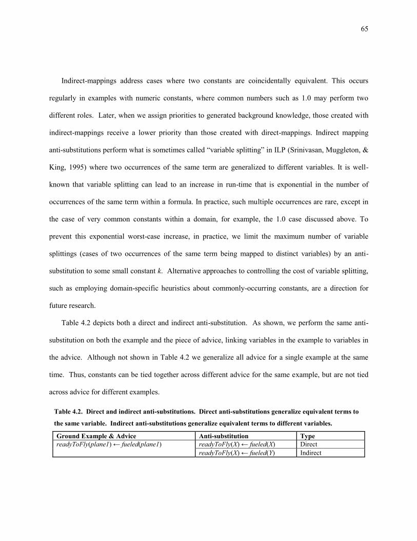
65

Indirect-mappings address cases where two constants are coincidentally equivalent. This occurs

regularly in examples with numeric constants, where common numbers such as 1.0 may perform two

different roles. Later, when we assign priorities to generated background knowledge, those created with

indirect-mappings receive a lower priority than those created with direct-mappings. Indirect mapping

anti-substitutions perform what is sometimes called “variable splitting” in ILP (Srinivasan, Muggleton, &

King, 1995) where two occurrences of the same term are generalized to different variables. It is well-

known that variable splitting can lead to an increase in run-time that is exponential in the number of

occurrences of the same term within a formula. In practice, such multiple occurrences are rare, except in

the case of very common constants within a domain, for example, the 1.0 case discussed above. To

prevent this exponential worst-case increase, in practice, we limit the maximum number of variable

splittings (cases of two occurrences of the same term being mapped to distinct variables) by an anti-

substitution to some small constant k. Alternative approaches to controlling the cost of variable splitting,

such as employing domain-specific heuristics about commonly-occurring constants, are a direction for

future research.

Table 4.2 depicts both a direct and indirect anti-substitution. As shown, we perform the same anti-

substitution on both the example and the piece of advice, linking variables in the example to variables in

the advice. Although not shown in Table 4.2 we generalize all advice for a single example at the same

time. Thus, constants can be tied together across different advice for the same example, but are not tied

across advice for different examples.

Table 4.2. Direct and indirect anti-substitutions. Direct anti-substitutions generalize equivalent terms to

the same variable. Indirect anti-substitutions generalize equivalent terms to different variables.

Ground Example & Advice Anti-substitution Type

readyToFly(plane1) ← fueled(plane1) readyToFly(X) ← fueled(X) Direct

readyToFly(X) ← fueled(Y) Indirect

66

In some cases, it is important that a constant seen in the ground advice remain constant in the final

generated background knowledge. For instance, staying with our readyToFly concept, if the teacher

provides advice such as flightInstrumentValue(tachometer) > 1000 it is probably important that

tachometer remain constant, as it would not make sense check if, say, the altitude is greater than 1000.

We use two techniques to determine when a constant in the advice should remain a constant in the

generated background knowledge. First, we allow the teacher to state “the constant tachometer should

remain constant.” In cases where the teacher does not provide this hint, we attempt to identify possible

constants through a simple algorithm. For each constant occurring in the original advice, we evaluate the

piece of advice with all other constants generalized against each example (positive examples for positive

advice or negative examples for negative advice.) If the piece of advice holds for m examples, we assume

that the constant should remain a constant in the generalized version of the advice. Here m is a tunable

parameter based upon the total number of example in the training set.

In some cases, this approach will either fail to identify values that should remain constant or will

determine a value should be held constant when it should not. One approach to handling these errors is to

create multiple generalizations, not variablizing the constant in one and variablizing the constant in

another. In this approach, we would assign a priority to each generalization so that the ones we

determined to be more likely could be searched first. However, in cases where a single piece of advice

contains multiple constants, this leads to exponentially many different generalizations. When this occurs,

we limit the number of resulting generalization to some small constant k.

When teacher provides advice about negative examples, the advice may be ambiguous. Imagine a

teacher says an example is negative because color = blue. Does this mean the example is negative

because it is blue or because it is not? Since the teacher is talking about specific examples that are

observable by our learning algorithm, we address this in an obvious way. Namely, we evaluate the

teacher’s statement on the current example, and we then, if necessary negate the advice so that it says

67

something that is true. Hence, if the current example is red, we would adjust the advice about color to be

color blue.

4.1.2 Standarizing Advice

Given the generalizations from the first phase, the second phase of

GENERATEBACKGROUNDKNOWLEDGE (lines 15 to 20) performs a unification to merge variables that

arose from constants found in the target literal (e.g., readyToFly(X).) For instance, if we consider the

direct anti-substitutions of all pieces of advice from Table 4.1, we have ( ) ( ),

( ) ( ),19 and ( ) ( ). After the unifications,

the implications would be ( ) ( ) ( ) ( ) and

( ) ( ) where X is shared. This allows distinct constants from different

examples that played the same role to be merged into a single variable.

4.1.3 Generating Background Rules

In the third phase (lines 22 to 30), we generate compound logical formulas by connecting the

generalizations for different pieces of advice with the AND and OR logical connectives. We generate

four different styles of formulas: per-piece, per-example, per-class, and “Mega Rules.” The per-piece

formulas correspond to the individual pieces of advice specified by the teacher. The per-example

formulas aggregate all the advice provided for a single example into one formula with the individual

pieces of advice joined via AND connectives. The per-example formulas allow the teacher to provide

many small pieces of advice about an example instead of requiring the teacher to compose a single

19 The fueled and gearDown advice pieces already use the same variable since they both came from advice attached to the same

example. As mentioned earlier, generalization for all advice attached to a given example occurs at the same time using the

same anti-substitution.

68

complex piece of advice. The per-class formulas combine via AND connectives either all of the positive

advice or all of the negative advice. Finally, Mega Rules attempt to capture all of the advice into one

logical statement, by conjoining direct-mapping generalizations of all advice from all positive and

negative examples.

More specifically, we do the following to produce our Mega Rules:

Let Fi be the logical formula that our algorithm produces by conjoining (“ANDing”) all of the

relevance statements about positive example i.

Let Gj be the logical formula that our algorithm produces by conjoining all of the relevance

statements about negative example j.

We make the following Mega Rules, where i ranges over the positive examples with advice and j over

those negative examples with associated advice:

( ) ( ) (4.2)

( ) ( ) (4.3)

( ) ( ) (4.4)

( ) ( ) (4.5)

The above are all ways to explain a collection of teacher-provided advice, though some are more

natural than the others. In the first one, our algorithm interprets the teacher as using each positive

example to provide aspects of a conjunctive concept and each negative example to state properties that

members of the concept lack (“this is a bird because it has wings, this other example is a bird because it

lays eggs, this third example is not a bird because it has leaves, this fourth example is not a bird because it

is made of metal. …”). The third and fourth lines are appropriate for disjunctive concepts (“Alice got to

work by taking the bus. Bob got to work by walking. … Carl did not make it to work because he slept all

day.”). In addition to the rules shown above, we also generate four additional Mega Rules in which we

negate positive advice and do not negate the negative advice.

69

When only direct-mapping generalizations exist, only a handful of formulas are generated, providing

excellent scalability. When indirect-mappings occur, we generate additional rules in which we substitute

all combinations of the indirectly-mapped advice pieces into the per-piece, per-example, and per-class

formulas. This process scales exponentially in the number of indirect-mapping generated. When this

occurs, we limit the number of resulting generalization to some small constant k.

4.1.4 Priority and Mode Assignment

In the final phase (lines 32 to 37) we convert each of the generated formulas back into an implication

(as a precursor to creating ILP background knowledge). During this phase, we assign a search priority

with a preference for longer formulas, i.e., those that use as much of the user-provided advice as possible.

Mega Rules receive the highest priority, followed by per-class and per-example formulas, and finally per-

piece formulas. It is these priorities that define the layers iteratively searched by our ONION algorithm

detailed in Chapter 6. Table 4.3 shows several of the implications generated for the sample concept.

The head of the generated clauses (e.g., rule1(X) or rule2(X) from Table 4.3) controls the logical

variables we exposed to the ILP algorithm during the search process. This is an important step as it

directly affects the effectiveness of our algorithm. In order to illustrate the importance of properly

Table 4.3. Generated Background Knowledge. Three types of background knowledge are created during

advice processing: per-piece, per-example, and mega-rule background knowledge. Per-piece is composed

of single pieces of advice. Per-example is composed of all advice piece for a single example. Mega-rules

use all provided advice combined via various logical operators.

Generated Background Knowledge Type Priority

rule1(X) ← fueled(X) gearDown(X) ¬ damaged(X) Mega-Rule High

rule2(X) ← ( fueled(X) gearDown(X) ) ¬ damaged(X) Mega-Rule High

rule3(X) ← fueled(X) gearDown(X) Per-Example Medium

rule4(X) ← ¬ damaged(X) Per-Example Medium

rule5(X) ← fueled(X) Per-Piece Low

rule6(X) ← gear(X, down) Per-Piece Low

70

exposing the correct logical variable in the generated rule’s head, consider a somewhat more complicated

readyToFly concept indicating that a plane has enough fuel to fly 1000 miles, defined logically as

( ) ( ) ( ) . (4.6)

A teacher might make the following statement about an example: “For , it is important

that ( ) ( ) .” Here, the teacher has essentially

specified how to calculate the range of the plane but has not giving advice about the range comparison.

Even though this is only partial advice, it is still valuable. Ignoring the head of the generated background

knowledge, our GENERATEBACKGROUNDKNOWLEDGE algorithm would produce the formula

( ) ( ) . (4.7)

Given this formula, Table 4.4 lists several of the rules that could be created, each with a different possible

head.

If we are trying to learn concept (4.6), rule1, rule2, and rule4 are not useful as they do not expose the

Range variable. Both rule3 and rule5 would be useful when learning the concept, although rule3 may be

considered more desirable since it provides all of the necessary variables and nothing extra. This

illustrates the importance of choosing the correct variables to expose in the head.

Algorithm 4.2 details the method used to selected the variables that we place in the head of the

generated clause along with the ILP modes for each of the variables. Essentially all of the variables tied

to the example during the generalization phase become input variables for the clause. As illustrated, it is

also advantageous to expose variables occurring in the body of the rule as output variables. However, the

size of the ILP search space increases exponentially in the number of variables exposed in the head of the

Table 4.4. Several possible background knowledge heads for the same rule body.


rule1(A) ← fuel(A, Fuel), mpg(A, MPG), Range = Fuel × MPG

rule2(A, Fuel) ← fuel(A, Fuel), mpg(A, MPG), Range = Fuel × MPG

rule3(A, Range) ← fuel(A, Fuel), mpg(A, MPG), Range = Fuel × MPG

rule4(A, Fuel, MPG) ← fuel(A, Fuel), mpg(A, MPG), Range = Fuel × MPG

rule5(A, Fuel, MPG, Range) ← fuel(A, Fuel), mpg(A, MPG), Range = Fuel × MPG

71

clauses, so it is infeasible to expose them all. In absence of other information, for each formula, we

expose only a single output variable. For any given formula, we determine the output variable by

considering all of the literals that we derived from positive pieces of advice and selecting the last variable

that was introduced (e.g., Range from above.) This approach scales well. However, in some cases,

variables that would be helpful may not be exposed in the head of the generate clause.

We assign input variables both an ILP input mode of ‘+’ (the argument must already be in the clause

being constructed) and a constant mode of ‘#’, plus we assign output variables both an output mode of ‘–’

(a new variable can be introduced) and a constant mode of ‘#’. Additionally, our algorithm also works

when the ground advice contains logical functions by generalizing the complete function into a single

variable (e.g., p( f(x, y ) ) generalizes to p(A) ) and generalizing the terms of the function, but not the

function itself (e.g., p( f(x, y ) generalizes p( f(A, B ) .)

Algorithm 4.2. DETERMINEHEADVARIABLES

1. Input:

2. A generalized clause of the form: e ⟵ A

3. from F’i on line 19 of Algorithm 4.1,

4. where e is the variablized example literal

5. and A is variable advice body consisting of one or more literals

6.

7. Ouput:

8. Head literal for generated background clause along with ILP modes

9.

10. Let ExampleVars = { v ∈ arguments of e | v is a logical variable } // Collect variables in e

11. Let BodyVars = { v ∈ arguments of literal in A | v is a logical variable } // Collect variables in body

12.

13. Let HeadVars = {} // Variables that will be in generated clauses head along with mode for variable

14.

15. For each var ∈ ExampleVars

16. If var ∈ BodyVars then

17. Let HeadVars = HeadVars { var }

18. Assign “input” (+) and “constant” (#) mode to var

19.

20. Let lastVar = last variable that occurs in a literal in A

21. If lastVar ∉ HeadVars then

22. Let HeadVars = HeadVars { lastVar }

23. Assign “output” (-) and “constant” (#) mode to lastVar

24.

25. Return HeadVars along with assigned modes

72

Clauses derived from formulas with OR connectives have the additional requirement that the selected

output variable must occur in all of the OR-ed subformulas. Determining whether a variable occurs in all

of the subformulas requires us to determine if two variables are equivalent. If argument-type information

(provided by the ILP modes) is available, we require only that type of the output variable match in all of

the subformulas. In the absence of typing information, we disallow output variables for disjunctive

formulas.

4.2 Experimental Results

We performed several experiments to demonstrate the performance of our background generation

algorithm. In addition to measuring learning performance on our test beds, we conducted comprehensive

empirical analyses to study the performance when there is noise in the labels on examples and when there

is noise in the advice. We designed these experiments to demonstrate the effectiveness of our algorithm,

its robustness to noise, and how the system is capable of generalizing advice about specific examples to

all the available examples leading to improved learning and accuracy. The improvements in

generalization performance can be significant, especially in the presence of a very small number of

examples.

We are interested in studying the behavior of our advice algorithm with respect to several criteria:

1. Its ability to learn diverse concepts across domains without the intervention of an ILP expert,

2. Its ability to effectively exploit teacher advice in order to learn concepts with only a small number

of examples,

3. Its robustness to teacher errors of commission in the examples (mislabeled examples),

4. Its robustness to teacher errors of omission in the advice (incomplete or missing literals).

Our experimental study consists of three experiments that we describe below.

73

4.2.1 Methodology

The experiments were all performed using the Bootstrap Learning testbed (see Section 3.1). We use

14 separate tasks from that domain during the experiments. The tasks all included third-party generated

training examples (up to 100 examples for each task) along with teacher advice for certain examples. The

mean accuracy of always guessing the majority category across each of these 14 tasks is 57%.

For each task we have 100 training examples and 100 test set examples. During our experiments, we

split the training set to generate a tuning set, used by the ILP system to evaluate parameter settings. For

runs with more than 25 examples, we place two-thirds of the data provided to our learner into a training

set and one-third the data into a tuning set. For runs where fewer than 25 training examples, we do not

use a separate tuning set, instead relying directly on training-set accuracy to tune parameters. In all

experiments we used an equal number of positive and negative examples.

Because there is an intended pedagogical order to the examples, some of which have associated

advice, we did not perform 10-fold cross validation within each lesson (in addition, since we have data

simulators, cross validation is not necessary – instead we simply use fresh samples of 100 examples as

our test sets). The results presented for each experiment are the test-set accuracies averaged over all 14

tasks. Across all of these tasks, we used the same parameter choices. That is, over all of the experiments

that we report here, our ILP system was run unchanged.

4.2.2 Results

Experiment A

In our first experiment, we compare the performance of our advice algorithm to the performance

without advice over all the 14 tasks. Figure 4.3 shows the results, where we plot learning curves, i.e.,

test-set accuracy as a function of increasing numbers of training examples. (As mentioned earlier, our

74

implementation is not an on-line, incremental learner. We simply run in “batch mode” for various

numbers of training examples.)

In the case where the learner is not given any advice, the ILP system is able to generalize across tasks

and domains, and obtain an average test-set accuracy of 74.0% when using all 100 training examples.

Even when using smaller fractions of training data, the performance without advice exceeds 57%, the

equivalent to the test set accuracy produced by random guessing. The main results in Figure 4.3 however,

are the test-set accuracies achieved in the presence of advice. Even when using only four training

examples per lesson, our algorithm achieves an average test-set accuracy of 93.8%, and reaches 100%

with only ten examples.

Experiment B

Experiment A involved advice from a 3rd

party who was careful to create rich and accurate advice.

However, real teachers are likely to make errors. In our 2nd

experiment we simulate errors of omission by

dropping literals from advice. We randomly drop literals as follows. For each advice rule we flip a

Figure 4.3. Experiment A: Testset accuracy as a function of the number of training, with and without

advice, averaged over 14 tasks.

0.00

0.25

0.50

0.75

1.00

0 25 50 75 100

Test

set

Acc

ura

cy

Number of Training Examples

With Advice

Without Advice

75

weighted coin, and it if comes up ‘heads’ we delete the last literal in the rule. If we deleted the last literal,

we flip the coin again and consider deleting the second-from-last literal; this continues until either the

rule’s literals are exhausted or the coin comes up ‘tails.’ In the later case, we place the possibly truncated

advice rule in our noisy advice set. We choose to remove from the end of advice rules, since prefixes of

conjunctive rules are likely to be partially coherent, whereas dropping literals from the middle of multi-

literal (i.e., conjunctive) statements may lead to nonsensical advice. A topic for future research is to

create more realistic models of imperfect advice.

Figure 4.4 shows the results of our errors-of-omission experiment, where we plot the test-set accuracy

as a function of the probability of randomly removing each literal as specified above. For each selected

probability-of-removing, we generated 30 independent “noisy” advice sets for each of our 14 lessons.

The impact of noisy advice depends on the number of training examples, so we perform this experiment

using 4 and 100 training examples.

Figure 4.4. Experiment B: Impact of errors of omission in advice. The x axis indicates the probability

value used in the advice-removal process (see text).

0.00

0.25

0.50

0.75

1.00

0.00 0.25 0.50 0.75 1.00

Test

set

Acc

ura

cy

Probability of Dropping Advice Literals

4 Training Examples

100 Training Examples

76

For both the training set with 4 examples and 100 examples, the test set performance exhibit similar

behavior, with the accuracy dropping steadily as increasing fractions of advice literals are removed.

However, with advice-omission rates as high as 50%, and with a small number of examples, our

algorithm produces average test-set accuracies of over 80%. This demonstrates that even partial advice

can be effective for learning, and we are able to leverage this information effectively even in the presence

of significant imperfections in advice.

Experiment C

In this final experiment, we compare the performance with and without advice in the presence of

mislabeled training examples. Figure 4.5 shows the results; we plot test-set accuracy as a function of the

percentage of mislabeled examples. We generate the noisy examples by first removing examples that

have advice attached from the set of training examples. With the remaining training examples, we

randomly select a fraction of the examples and flip their labels. We then return the examples with

attached advice to the training set. We took care to guarantee that the final fraction of mislabeled

examples was correct when the examples with advice added back into the training set. This approach to

noise generation limited the range of noise available, especially for small training sets. For instance, if we

have a training set size of four and two of those are examples with advice attached, the minimum amount

of noise that can be considered is 25% (the result of flipping a single, non-advice, example).

For experiment C, we generate 30 independent sets of mislabeled examples and, separately, ran with

and without advice using each of these noisy data sets. The results are averaged over all random 30 runs

and over all 14 tasks. As expected, the example noise reduces the performance of both the advice-free

and with-advice cases. The main result from Figure 4.5 is that our advice algorithm, combined with the

ONION, performs well even in the presence of large amounts of data noise. In contrast, the no-advice case

degrades more quickly about the level of random guessing (50%).

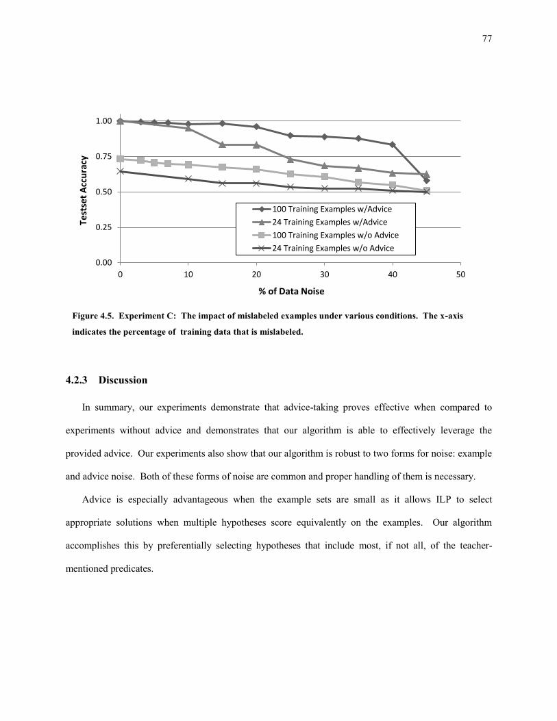
77

4.2.3 Discussion

In summary, our experiments demonstrate that advice-taking proves effective when compared to

experiments without advice and demonstrates that our algorithm is able to effectively leverage the

provided advice. Our experiments also show that our algorithm is robust to two forms for noise: example

and advice noise. Both of these forms of noise are common and proper handling of them is necessary.

Advice is especially advantageous when the example sets are small as it allows ILP to select

appropriate solutions when multiple hypotheses score equivalently on the examples. Our algorithm

accomplishes this by preferentially selecting hypotheses that include most, if not all, of the teacher-

mentioned predicates.

Figure 4.5. Experiment C: The impact of mislabeled examples under various conditions. The x-axis

indicates the percentage of training data that is mislabeled.

0.00

0.25

0.50

0.75

1.00

0 10 20 30 40 50

Test

set

Acc

ura

cy

% of Data Noise

100 Training Examples w/Advice

24 Training Examples w/Advice

100 Training Examples w/o Advice

24 Training Examples w/o Advice

78

4.3 Related Work

ILP research has a rich history of developing systems capable of initiating human-computer

interaction and using them guide and constrain the search. The most notable such systems include

MARVIN (Sammut, 1981), MIS (Shapiro, 1983), DUCE (Muggleton, 1987), CIGOL (Muggleton &

Buntine, 1988) and CLINT (De Raedt, 1992) where the algorithm can ask the human one or more

questions that would guide the search. For instance MIS relied on the human answering queries by

providing the labels of examples, together with a proof, or derivation, for each positive response. In

contrast, in our present work the human initiates the input by providing advice, either in general or in

association with the original training data.

Another general area of related work is theory refinement or theory revision (e.g., Mangasarian,

Shavlik, & Wild, 2004; Pazzani & Kibler, 1992; Srinivasan, 2001) where the user provides an initial

logical theory that explains many and not all examples, and the learning system must modify this theory.

As a result the search is constrained to prefer theories close to the original theory, similar to the present

work. But a key distinction is that the advice in our present work is example-specific, which can

substantially ease the burden on the user, as compared to expressing abstract rule(s) underlying the

concept.

Our work is closely related to argument-based machine learning ABML (Mozina, Zabkar, & Bratko,

2007) that takes as input user-provided advice about specific examples, in the form of an argument. A

key distinction is that the present work does not assume the arguments are exactly correct and therefore

may combine various pieces of different arguments in order to construct rules. Another distinction is that

to our knowledge ABML has been applied strictly to propositional-rule learning.

79

4.4 Conclusions and Future Work

Not surprisingly, teacher advice is useful to learning. The key challenge is the need to generalize hints

and advice the teacher gives about specific examples so that it accurately applies to future examples. We

present a formal approach to incorporating this into the wider framework of ILP. The empirical results

show that our system is able to learn well, across multiple concepts, from a combination of training

examples and teacher-provided hints. Running our ILP system without these hints − i.e., only using the

training examples – also produces reasonable accuracies on held-out (“test set”) examples. Another key

challenge is effective parameter selection and the automation of the ILP-setup task. The final challenge is

to ensure that the system is robust to noise, both in examples and in advice.

We evaluated our algorithms, holding all default parameter settings constant, on 14 tasks from two

domains designed by third-parties not under our control; these human teachers provided training

examples as well as relevance information. In our experiments, we demonstrated that our system is

capable of (1) effectively automating the ILP-setup task over different tasks from significantly different

domains, (2) exploiting teacher hints and relevance information to learn concepts with near-perfect test-

set accuracies even if given only a small set of training examples, (3) being robust to example-label noise

that can arise from teachers’ errors of commission, and (4) being robust to advice noise that is likely to

arise from teachers’ errors of omission.

One possible future direction is to look further at exploiting teacher-provided feedback beyond

statements about which features and objects are relevant, such as allowing teachers to provide corrections

to previous advice statements. Another is to explore the possibility of refining the learned theories using

teacher feedback along the lines of theory refinement for ILP (Mozina, Zabkar, & Bratko, 2007;

Muggleton, 1995; Oblinger, 2006; Pazzani & Kibler, 1992; Richards & Mooney, 1995). Refining

teacher's advice is important as it renders the ILP systems more robust to teacher errors that occur

naturally in human teaching. Another direction is deploying our approach in the context of probabilistic-

80

logic learning (Getoor & Taskar, 2007). A final appealing direction of this research is to embed it into

some user interface where a human can train their software by a combination of making simple English

statements, pulling down menus, selecting items, and gesturing at objects (e.g., clicking with the mouse)

to indicate relevance and objects of discourse (“this object should not be near that one”).

81

5 Advice Acquisition via a Human-Computer Interface

As I demonstrated in Chapter 4, it is possible to design an Inductive Logic Programming (ILP)

system that facilitates the use of ILP by non ILP experts, allowing domain experts, with no ILP

experience to use ILP. However, the algorithm presented in Chapter 4 still required some understanding

of the advice format used by the algorithm and understanding of basic logic. Although I do not believe

these requirements are onerous for the user, it would be even more advantageous to allow the same

information to be collected through a human-computer interface (HCI).

In this chapter, I outline an interactive learning process and examine the use of an HCI to further

facilitate the use of ILP. The HCI provides a way for the user to specify relational knowledge about

specific examples. I demonstrate the approach's effectiveness by examining the task in the Wargus real-

time strategy game (Wargus, 2002). I providing a simple GUI through which a domain expert can specify

relational advice explaining various scenarios and show that combining the HCI and a suitable advice-

taking learning algorithm is effective. I compare successfully against both (a) using no advice and (b)

hand-written advice.

I am not the first to demonstrate an HCI for knowledge acquisition. Extensive research exists

studying HCIs for this purpose. Some approaches rely on demonstration by the domain expert of some

process (Chen & Weld, 2008; McDaniel & Myers, 1999). Others provide an interface in which the expert

may specify additional examples to guide or correct the learning algorithm (Vander Zanden & Myers,

1995). Some treat domain knowledge as a form of constraints and provide an interface to specify those

constraints (Huang & Mitchell, 2006). However, my method is the first to look at automatically obtaining

relational knowledge and then automatically integrating that knowledge with an underlying ILP learning

system. The HCI approach to obtaining relational knowledge in a ground format, automatically

82

processing it into the required knowledge representation, and immediately using the knowledge to

perform ILP learning is, I believe, unique to this research.

Much of the work presented in this chapter was performed in collaboration with several others and

presented in “Integrating Knowledge Capture and Supervised Learning through a Human-Computer

Interface” (Walker, Kunapuli, Larsen, Page, & Shavlik, 2011) at the 6th International Conference on

Knowledge Capture.

5.1 Overview of Approach

We consider a learning paradigm designed to assist domain experts (we will also refer to them as

users) in the process of creating and refining domain knowledge through the use of an HCI. We view

domain knowledge as a form of advice provided by the user to the learning algorithm. We also consider

advice acquisition to be an iterative process (see Figure 5.1) of a user specifying advice, an algorithm

learning a model, a user reviewing results, and a user refining or augmenting the advice. Although this

paradigm applies to many forms of learning, we specifically consider supervised learning algorithms that

take as inputs both training examples and additional domain knowledge.

Our iterative learning process proceeds in four stages. First, we present an HCI through which the

user specifies advice. Our HCI accomplishes this by displaying information about a single training

example and asking the user to “explain” why that example was positive (or negative). We specifically

consider advice in the form of concrete logical statements, as discussed in Chapter 4. For instance, in a

medical domain, the HCI might display with a patient’s information, health history, etc. and ask the user

why that patient was high risk for heart problems. The user might have the domain knowledge that the

patient was a high risk because “the patient’s cholesterol was high during her last visit and her father’s

family has a history of heart disease.” Through the HCI, the user would be able to express this

knowledge without understanding the required representation or even formal logic.

83

After the user finishes entering advice for a number of training examples, the second phase of our

process translates the advice into a form usable by the learning algorithm. This usually entails

generalizing the advice and possibly changing the representation of the advice to the form used by the ILP

algorithm. The process of converting the advice can be quite complex and often there are multiple

generalizations with distinct meanings. Since we do not expect the user to understand the underlying

representation of the advice, it is often infeasible to ask the user to correct the advice directly and we

instead rely upon our iterative process to indirectly improve the advice.

Phase three of our process performs the actual learning. At this point, we provide to the learning

algorithm both the training examples and the generalized advice. The learning algorithm then produces a

model. After learning, we pass this model onto phase four. Here, we evaluate the model against

additional examples and present an HCI allowing the user to review the effectiveness of the model.

Advice-TakingHCI

Learning Algorithm

Advice Processor

HCI to evaluate learned model

Training Examples

GroundAdvice

Generalized Advice

Learned Model

Refineor

Extend Advice

Figure 5.1. Our human-computer learning paradigm. Initially the user specifies advice through an HCI.

Then the advice is processed and learning occurs. Afterward the results are presented to the user via an

evaluation HCI. The process iterates until the user is satisfied with the results.

84

The reviewing HCI presents the user information about which test-set examples were correctly or

incorrectly predicted by the model. Based on this, the user may elect to return to phase one in order to

adjust previously presented advice, provide new advice, or label new examples. In addition to being used

as part of an iterative learning process, the review HCI, especially when coupled with a probabilistic

learning algorithm, can be used for other applications, as discussed in Section Error! Reference source

not found..

5.2 Intelligence, Surveillance and Reconnaissance – A Motivating Application

When designing the Wargus tower-defense task used as a basis for this research, our goal was to

design an application that demonstrated the use of advice-taking, learning, and an HCI for intelligence,

surveillance, and reconnaissance (ISR). ISR refers to the integration of analysis and planning

(intelligence) with the operation of passive sensors (surveillance) and active intelligence gathering assets

(reconnaissance). For instance, one common ISR application entails the analysis of satellite imagery to

plan and execute reconnaissance via unmanned drones during military operations. Similarly, the

integration of video surveillance and the dispatching of law enforcement units falls under the ISR

umbrella. In a typical ISR application, large amounts of surveillance information is gather and passed off

to analysts who must look through the data to identify important events. Once identified, reconnaissance

or other actions are planned accordingly.

ISR provides an excellent testbed for integration of advice-taking, learning, and an HCI due to the

massive amount of data generated by the wide-spread surveillance capability currently deployed.

Analyzing all the data is often beyond the limited resources of human analysts. Pre-filtering the gathered

surveillance reduces the amount of human analysis required, allowing more data to be processed in less

time.

85

However, learning the appropriate model to enable this filtering requires an extensive amount of

domain knowledge. What constitutes an interesting scenario, i.e., one that a human analysis must

examine, may depend on numerous factors; learning with only positive and negative examples can be

challenging and the difficulty of this learning task may be reduced through the utilization of domain

knowledge. However, as discussed throughout this document, the domain expert (i.e., the analyst) often

does not have the skills necessary to provide the knowledge in a way usable by the machine learner.

Figure 5.2 depicts the training and real-world usage phases in an ISR application. During the

“learning phase” an analyst categories interesting images and provides advice through an HCI. From this,

a probabilistic learning algorithm learns a model and allows the analyst to further refine the model

through additional advice. After the analyst determines the model is accurate enough, in the “real-world

use” phase, the model sorts incoming images according to the probability they are interesting, presenting

the most interesting images to the analyst. The analyst then dispatches reconnaissance appropriately.

One important aspect of an ISR application is the use of a probabilistic algorithm. A probabilistic

model allows incoming surveillance to be sorted according to how likely it is to be interesting. Without

this aspect, only a coarse (i.e., binary) categorization could be performed and the analyst would have to

examine far more images.

We designed the Wargus tower-defense task to be a simple ISR application. We consider scenarios

interesting if the tower falls, as these are the situations in which reconnaissance might be necessary to

determine further the amount of risk the tower was in. In this chapter we look at the advice-taking aspect

of the ISR application in the Wargus domain.

5.3 Our Advice-Taking HCI

In this section we provide details of a prototype HCI we created to take advice in the Wargus tower-

defense task, discussed in Section 3.2 and depicted in Figure 5.3. The goal of this prototype was to both

86

demonstrate the effectiveness of an HCI in the Wargus task. Figure 5.4 depicts the simple prototypical

GUI we designed and used to gather relational advice.

In general, the design of the HCI depends greatly upon the type of the knowledge being gathered and

the task for which the knowledge is being provided for. Although our prototype HCI is specific to the

Wargus task, conceptually, many of the same design elements would be required for other tasks.

Surveillance

Probabilistic learning algorithm

Analyst provide advice through HCI

Analyst reviews model via HCI

Images

Learned Model

Refineor

Extend Advice

Analyst categorizes images as

“interesting” or “uninteresting”

Training examples

HCI presents sorted list of the most

interesting images to analyst

Analyst plans and dispatches

reconnaissance Images

Learnin

g Ph

ase

Real-w

orld

Use

Figure 5.2. Intelligence, surveillance and reconnaissance (ISR) learning and usage scenario. During the

“learning phase” an analyst categories interesting images and provides advice through an HCI to train a

probabilistic model. In the “real-world use” phase, the model sorts and filters incoming images according

to the probability the are interesting, presenting the most interesting images to the analyst. The analyst

then dispatches reconnaissance appropriately.

87

5.3.1 Elements of our Advice-Taking HCI

In our approach, the user provides advice through the following process:

1. An example is selected, either manually by the user or through some automatic process.

2. The HCI provides the user (ideally visually) information about the example.

3. The user provides advice through the HCI to explain why this example was either positive or

negative.

4. The user either returns to Step 1 to provide more advice or stops.

In order to facilitate this process, our HCI needs to:

Provide information about specific examples.

Allow selection and naming of entities or groups of entities.

Provide a method to indicate relations among selected entities.

Allow the user to review, and possibly edit, previously specified advice.

DefendingTower

AttackingArcher

AttackingSwordsman

Figure 5.3. The Wargus tower-defense task. Multiple attacking units, consisting of swordsmen, archers,

and ballista, assault the defender’s tower. Depending on the composition of the attacking force, the tower

will survive or be destroyed. The Wargus tower-defense learning task involves predicting which of these

outcomes will occur.

88

Providing Example Information

The HCI must provide information to the user about examples. In our knowledge-capture approach,

each advice statement is about a specific example. Thus, the HCI needs to provide at least the

information about one example. In the Wargus tower-defense game we can depict all information about

an example as a picture of the game board. In some domains, this is not possible or not desirable.

Figure 5.4. Prototype GUI for advice taking in Wargus. The GUI consists of four sections: (upper-left)

entity selection and naming, (upper-right) display of current game board, (lower) controls specifying

relations between selected entities, and (not shown) a list of previously specified advice.

89

Selecting and Naming Entities

Advice in our system consists of relations among entities. Here, an entity is any object in the domain.

For instance, in the Wargus domain, the various units on the game board are entities. A user needs a

method to indicate the entities that should be related. Thus, we require some sort of entity-selection

mechanism. The entity-selection methodology will different depending on the domain. In board game

domains, such as Wargus, simply clicking on one or more entities is sufficient. However, for other

domains, a much more complex approach may be necessary.

One extension we found particularly useful in our Wargus GUI prototype was the ability to name

groups of entities. When selecting entities in Wargus, by default we named single entities either THIS or

THAT. When selecting groups of entities, the default names are THESE or THOSE. Thus, later on, when

specifying a particular relation, we could state THIS is related to THAT or THESE are related to THAT.

However, in order for this approach to work, the underlying task must be able to understand these entity

grouping. In the Wargus domain, background knowledge exists facilitating this. For instance, the

count/220 predicate supports sets of entities.

Specifying Relations

In addition to selecting entities, in many domains, objects have additional properties. For instance, in

the Wargus domain, all units have a property indicating its x-y location. Thus, a mechanism is required to

access the properties.

In relational logic, we specify relations through predicates. For instance, isNearTo(archer1, tower) or

colorOf(archer1, green). The HCI needs to know what predicates the user may use to specify relations.

Here, the complexity of the HCI will depend greatly on the complexity of the domain. Our Wargus

20 As mentioned previously, count/2 represents the set of literals with a predicate symbol of “count” and two arguments.

90

domain contains only binary relations, so we provide drop-down menus to the entity-relation-entity

information.

Our ground advice format allows conjunctions, disjunctions, and negations. Thus, the HCI must also

support specifying advice with these logical connectives. In our prototype, we provide the negation of all

predicates in the “relation” menu. A button provides the ability to create conjunctions of multiple

relations. Disjunctions are implied implicitly between different pieces of advice. However, as discussed

in Chapter 4, the advice algorithm tries several combination of the user-provided advice statement. This

further relieves the user from understanding the exact ILP algorithm while allowing the user to specify

advice in a variety of ways.

Editing Advice

From a usability standpoint, allowing the user to edit previous provided advice is important. While

our GUI allows for some simple editing of the current piece of advice and the viewing of previously

provided advice, it does not allow the user to edit previous advice. While this is an integral part of the

HCI, I do not explore this aspect of the HCI other than to mention that while using our GUI, we often

examine the previous advice to determine if we needed to state something new or not.

5.3.2 A General HCI implementation

Above we showed a prototype HCI customized to a specific task, namely the Wargus tower defense

game. While this specialized HCI allowed us to investigate the requirements of an advice-giving HCI and

determine the usability of a GUI for providing advice, we believe that a more general approach would

also be effective. Figure 5.5 sketches one possible general HCI for advice-giving. In this HCI, the user

would be presented a set of the known relations about an example. In ILP, the relations form a graph,

chaining from one relation to another through the arguments of the various relations. The nature of the

relational structure allows the GUI to present the relations in an easy to understand format. To specify

91

advice, the use would simply drag the relevant relations from the graph. This general HCI, while perhaps

non-optimal for some tasks, would provide non-experts an accessible method to writing advice.

One of my research goals is to make ILP more accessible to the non ILP expert user. This general

HCI approach would help fulfill that goal by further abstracting the details of the underlying ILP system.

Since this general approach is not task specific, it requires no ILP expert and could be provided as part of

an ILP system.

hadHeartAttack(pat1)

appointment(pat1, app1)

lastAppointment(pat1, app3)

dob(pat1, 1/12/1947)

relation(familyP1, mother)

appointment(pat1, app9)

…

history(pat1, familyP1)

history(pat1, familyP6)

…

hadHeartAttack(familyP1)

…

bloodPressure(app1, 90, 140)

cholesterol(app1, 295)

weight(app1, 295)

…

Patient 1 Relations

Why did patient 1 have a heart attack?

lastAppointment(pat1, app3) cholesterol(app3, 310) AND

Drag new relation here to extend advice...

hadHeartAttack(pat1)

Figure 5.5. Sketch of a general ILP advice-giving HCI. One area of the GUI (top) displays a graph of

relations known about an example, while the another area (bottom) allows the user to construct advice by

dragging relations from the relation graph. While not optimal for all domains, this general HCI would

enable advice to be provided without the creation of task-specific GUI.

92

5.4 Generating Generalized Advice and Learning with It

Next we look at an advice-processing approach that converts the ground advice obtained through the

advice-taking HCI into background knowledge in the form of generalized Horn clause. Several relational

learning algorithms, such as various inductive logic programming approaches and the boosted relational

dependency network (bRDN) algorithm described in Section 2.2.5, use a Horn-clause representation for

background knowledge and can use such generated background knowledge directly.

Output from our advice-taking HCI is represented as a set of ground logical implications. As shown

in Table 5.1, the consequence of a piece of advice states the category of a specific training example. The

antecedent is a conjunction of literals defined within the domain (either as 'raw' features or via

background rules). We transform the ground advice into generalized Horn clauses using the advice-

handling process presented in Chapter 4. As discussed previously, this algorithm take advice in a ground

format, generalizes the advice, and creates background knowledge representing various combinations in

the form of (1) “per-piece” advice by considering each advice statement independently, (2) “per-example”

advice by conjoining all of the advice specified for a given example into a single combination, (3) “per-

class” advice by conjoining all of the positive advice or all of the negative, and (4) “mega-rules” as shown

in Table 5.1.

5.5 HCI for Reviewing Learned Models

In addition to providing an accessible way for users to provide advice, an HCI provides an intuitive

way to present the results of learning to the user. For instance, as discussed previously and shown in

Figure 5.1, an HCI could provide a method for the user to review the results of learning and to correct

previously provided advice or augment the advice based upon the errors of the learned model.

93

Figure 5.7 shows a prototype HCI we designed to review the results of learning in Wargus. This

simple HCI displays a visual representation of a set of examples, along with the categorization assigned

by the learned model. In our prototype Wargus HCI, we use boosted Relational Dependency Networks

(bRDN) as a learning algorithm (Natarajan, Khot, Kersting, Gutmann, & Shavlik, 2010). BRDNs provide

a probabilistic classification algorithm. As seen in the figure, this allows our HCI to order the examples

according to predicted probability of the class. Probabilities allow two interesting applications: 1) error

correction by providing additional or refined advice and 2) filtering examples according to their

probability.

In an error-correction application, the review-results HCI presents examples that have been

misclassified, ordered according to how misclassified the examples were. This allows the user to see the

examples that the model has the most trouble classifying correctly, i.e., how highly probable negative

examples were predicted to be and how improbable positive examples were predicted to be.. The user

can then provide additional advice attached to those particular examples to help the learner with those

particular examples. Alternatively, the HCI could present example that were misclassified by a small

margin for review. This approach focuses more on the “hard” examples and is a common practice in

Table 5.1. Generated background knowledge for some simple ground advice. Initial ground advice is first

generalized. Then various combinations are generated representing possible guesses at the meaning of the

set of advice statements.

Description Advice

Initial ground advice ex(pos1) ← p(pos1) q(pos1).

ex(pos1) ← r(pos1).

ex(pos2) ← s(pos2).

“Per-piece” advice a1(E) ← p(E) q(E).

a2(E) ← r(E).

a3(E) ← s(E).

“Per-example” advice e1(E) ← p(E) q(E) r(E).

e2(E) ← s(E).

“Per-class” advice c1(E) ← p(E) q(E) r(E) s(E).

“Mega” advice m1(E) ← p(E) q(E) r(E) s(E).

m2(E) ← p(E) q(E) r(E) s(E).

94

active learning (Settles, 2008). The error-correction application is an integral part of the human-

computer learning paradigm discussed earlier and provides the functionality necessary for the last stage of

the process depicted in Figure 5.1.

A second interesting application for the model-review HCI is presenting filtered examples. In many

applications, the amount of data exceeds the ability of the user to examine the data. For instance, as

discussed previously, in Intelligence, Surveillance and Reconnaissance (ISR), it is advantageous to

identify examples that are interesting in some way. The Wargus TowerFalls task embodies this type of

application, here the interestingness corresponds to how likely the tower will fall. In the filtering

application, the model-review HCI becomes a tool were only the examples with the highest model-

predicted probability are displayed. These examples are the ones model deemed most interesting and are

likely to be the ones that analysts need to examine in detail.


In order to evaluate our HCI and advice-taking approach we performed experiments using the Wargus

tower-defense game. We are interested in the effectiveness of advice generated using our advice-taking

HCI versus both hand-written advice and using no advice.

Our initial goal is to determine whether our HCI is capable of representing the types of advice a user

might like to say in general. To evaluate that, we had group members who were not directly involved

with Wargus nor its HCI (a) watch Wargus games, (b) learn some basic strategy, and then (c) provide

advice in ordinary English describing why a tower fell or stood for 5-10 specific initial states of our

Wargus game.

A vast majority of the natural language advice was given in terms of the numbers and types of units in

the attacking force. Overall, users provided 311 sentences of advice about 100 examples. Table 5.2

contains some general statistics gleaned from the natural language advice provided by the users. Users

95

usually tended to give specific advice in terms of certain features such as numbers of units, the presence

or absence of a moat, and whether or not the there was a ballista in the attacking force. For instance, "five

archers are sufficient to destroy the tower," or conjunctive advice: "there is a moat and only footmen;

hence the tower stands." We used this collected natural language advice to guide the design decisions of

what we enabled the user to state in the final version of our HCI prototype.

Figure 5.6. A prototype Wargus HCI used to review the predictions of the learned model.

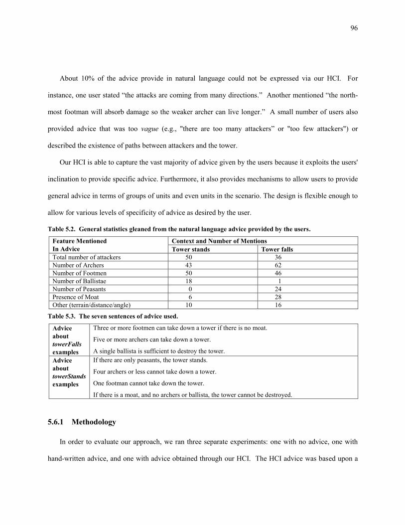
96

About 10% of the advice provide in natural language could not be expressed via our HCI. For

instance, one user stated “the attacks are coming from many directions.” Another mentioned “the north-

most footman will absorb damage so the weaker archer can live longer.” A small number of users also

provided advice that was too vague (e.g., "there are too many attackers” or "too few attackers") or

described the existence of paths between attackers and the tower.

Our HCI is able to capture the vast majority of advice given by the users because it exploits the users'

inclination to provide specific advice. Furthermore, it also provides mechanisms to allow users to provide

general advice in terms of groups of units and even units in the scenario. The design is flexible enough to

allow for various levels of specificity of advice as desired by the user.

5.6.1 Methodology

In order to evaluate our approach, we ran three separate experiments: one with no advice, one with

hand-written advice, and one with advice obtained through our HCI. The HCI advice was based upon a

Table 5.3. The seven sentences of advice used.

Advice

about

towerFalls

examples

Three or more footmen can take down a tower if there is no moat.

Five or more archers can take down a tower.

A single ballista is sufficient to destroy the tower.

Advice

about

towerStands

examples

If there are only peasants, the tower stands.

Four archers or less cannot take down a tower.

One footman cannot take down the tower.

If there is a moat, and no archers or ballista, the tower cannot be destroyed.

Table 5.2. General statistics gleaned from the natural language advice provided by the users.

Feature Mentioned

In Advice

Context and Number of Mentions

Tower stands Tower falls

Total number of attackers 50 36

Number of Archers 43 62

Number of Footmen 50 46

Number of Ballistae 18 1

Number of Peasants 0 24

Presence of Moat 6 28

Other (terrain/distance/angle) 10 16

97

representative sample of seven sentences (Table 5.3) expressed in natural language (we selected these

seven sentences before running any experiments and did not modify them during the course of our

experiments). We only used relations that could be entered through the HCI; we disregarded the rest of

the natural language advice.

Table 5.4 shows some of the ground advice generated via the HCI. After creating the ground advice

through the HCI, we used the advice generalization algorithm described previously to generate a set of

background clauses, resulting in 21 separate pieces of background knowledge including the per-piece,

per-example, and mega rules. While our advice taking learner can accept advice expressed in predicate

calculus, the full richness of first-order logic was not needed to capture the human-provided advice.

We created the hand-written advice (see Table 5.5) without using the HCI, representing what a

domain expert who understood the required knowledge representation would create, writing the advice

directly as seven Horn clauses. Once we created the advice, we used the boosted relational dependency

network (bRDN, Section 2.2.5) algorithm to learn a model predicting whether the towers would stand or

fall. All learning was performed using the same parameters for the bRDN algorithm.

Table 5.4. Sample ground logical statements about the Wargus tower-defense game for one positive (pos1)

and one negative example (neg1).

Example Advice

towerStands(pos1) count(archers, pos1) = 0

count(footman, pos1) = 0

count(ballista, pos1) = 0.

count(archers, pos1) ≤ 4.

count(footman, pos1) = 1.

moatExists(pos1)

count(archers, pos1) = 0

count(ballista, pos1) = 0.

towerStands(neg1) count(footman, neg1) ≥ 3.

count(archers, neg1) ≥ 5.

count(ballista, neg1) ≥ 1.

98

We evaluated the learned models for the three separate experiments against a held-aside set of 900

testing examples and produced learning curves comparing the performance of (a) no advice, (b) hand-

written advice, and (c) HCI generated advice.

5.6.2 Results

Figure 5.7 shows the area under the ROC (AUROC) curve for the three experiments. We tested

significance of the results via the (two-tailed) sign test, a nonparametric test based on the binomial

distribution (Mendenhall, Wackerly, & Scheaffer, 1989). The sign test is an exact test (McNemar’s test is

an approximation that was historically used purely because of computational limitations). The null

hypothesis of the sign test is that both approaches are equally accurate; hence each test case for which the

two approaches make different predictions is viewed as the flip of a fair coin. An approach “wins” such

as test case if it predicts correctly and the other approach predicts incorrectly. Where there are N test

cases for which the approaches give different predictions, and the most wins for either approach is h, the

computed p-value is the probability of at least h heads by either method under the binomial distribution

b(N,0.5), that is, in N flips of a fair coin.

Table 5.5. Hand-written advice about the Wargus tower-defense game. The actual advice submitted to

the ILP system consisted of seven Horn clauses directly representing the hand-written advice.

Example Advice

towerStands(World) count(archers, World) = 0

count(footman, World) = 0

count(peasants, World) ≥ 0.

count(archers, World) ≤ 4.

count(footman, World) = 1.

moatExists(World)

count(archers, World) = 0

count(ballista, World) = 0.

towerStands(World) count(archers, World) ≥ 0.

count(ballista, World) ≥ 1.

¬ moatExists(World)

count(footman, World) ≥ 3.

99

The difference in error rates between the HCI advice approach and the no advice approach is

statistically significant (p < 0.05) at every point in the curve, with p-values as low as 3.89 × 10-15

at the

largest difference in the curves (at 30 training examples). This demonstrates that, in this domain, the

HCI-generated advice does improve learning, especially in the early regions of the learning curve.

The difference in error rates when using the two different types of advice is significant only for a few

points in the curve, at 30, 70 and 100 examples. We consider this a positive result, as it indicates that our

HCI approach performed as well as hand-written advice.

In addition to the bRDN experiments, we also compared using the HCI-generated advice with a

knowledge-based support vector machine (KB-SVN) (Fung, Mangasarian, & Shavlik, 2002) as the

learning algorithm. In a knowledge-based SVM, the advice is provided as a set of linear equations

dictating areas that should be either positive or negative. Since support vector machines, in their standard

formulation, work with fixed-length feature vectors, we converted all of the features in the Wargus tower-

Figure 5.7. Learning curve showing test set performance in the Wargus tower-defense game comparing

models learned with hand-written advice, HCI generated advice, and no advice. All models were learned

the using boosted relational dependency network algorithm. The HCI generated advice was generalized

using the techniques discussed in Chapter 4.

0.5

0.6

0.7

0.8

0.9

1.0

10 20 30 40 50 60 70 80 90 100

Are

a U

nd

er

the

RO

C C

urv

e

on

90

0 T

est

set

Exam

ple

s


HCI Advice

Hand Written Advice

No Advice

100

defense task into Boolean or real valued features. Additional, all of the advice had to be hand-translated

into a set of linear equations representing the advice in the correct format.

We compared advice and no-advice resulting in an SVM formulation by running experiments with a

vanilla SVM (i.e., no-advice) and a KB-SVM (i.e., advice). They results, shown in Figure 5.8, are similar

to the bRDN results, with the HCI advice outperforming the no-advice equivalent by a good margin early

in the learning curve.

5.6.3 Discussion

We performed these experiments to evaluate two factors: whether a GUI could be effectively used by

non ILP experts to create advice and whether the generated advice could be as effective as background

knowledge written by an ILP expert. As mentioned early, based on the natural language data we

collected, our GUI was able to represent 90% of the advice that users provided through natural language.

Thus, while not all desired advice could be specified, the users were able to create, through our prototype

Figure 5.8. Learning curve showing test set performance in the Wargus tower-defense game comparing

models HCI generated advice and no advice. Models were learned the using support vector machine

(SVM) and knowledge-based support vector machine (KB-SVM) algorithms, respectively.

0.00

0.10

0.20

0.30

0.40

0.50

0.60

0.70

0.80

0.90

1.00

10 20 30 40 50 60 70 80 90 100

Are

a U

nd

er

the

RO

C C

urv

e

on

90

0 T

est

set

Exam

ple

s


No Advice (SVM)

HCI Advice (KB-SVM)

101

GUI, the majority of the advice they would have stated if working with an ILP expert. Furthermore, the

effectiveness of the GUI provided advice compared favorably with the hand-written ILP expert advice.

This further shows effectiveness of the GUI in the facilitation of advice-giving for the Wargus task.

5.7 Background and Related Work

Extensive research exists studying domain expert knowledge acquisition through the use human-

computer interaction (Stumpf, Rajaram, Li, & Wong, 2009). Additionally, previous research examines

how to exploit domain knowledge obtained either through an HCI, generated algorithmically or by hand.

Other non-HCI methods exist. One method is programming by demonstration (Cypher, 1993). In

programming by demonstration, a domain expert performs a sequence of actions demonstrating how to

perform some task. From this demonstration, a learning algorithm builds a procedural program intended

to solve the task. Often, the learned programs must be adjusted through further interaction with the user.

One such system (McDaniel & Myers, 1999) allows the user “nudge” the system through the inclusion or

removal of training examples. Another approach (Chen & Weld, 2008) allows users to adjust the training

data directly, adding missing information after the demonstration process. Unlike our approach, both of

these system work directly with the training examples without accepting explicit background knowledge.

Some approaches do allow explicit background knowledge to be specified. For instance, Vander Zanden

and Myers (1995) provide a method to specify background knowledge, but require understanding of the

underlying knowledge representation represented in the Lisp programming language. Another method of

human-computer interaction is programming by example (Fails & Olsen, 2003; Lieberman, 2001). Here

the user provides a prototypical example of the desired result, such as the result from a database query.

These approaches again differ from our approach in that they operate on the examples not on additional

background knowledge.

102


My main goal in this document is to demonstrate that ILP can be used without expert ILP knowledge.

Advice-giving techniques, such as those seen in Chapter 4 reduce the difficult of using ILP. However,

they still require the user to understand the advice-giving format and limitations. In some ways, our

previous advice algorithm traded off the requirement that the user understand ILP with the requirement

that the user understand the advice-giving format. Allowing the user to specify knowledge as ground

advice about specific examples through a human-computer interface provides one appealing method of

overcoming this difficulty. Here I have demonstrated that an HCI can alleviate much of this additional

requirement. The HCI provides a process through which the user can easily provide advice as also

guarantees that the advice conforms to the limitations of the underlying advice processing algorithm.

I also believe that the HCI process provides a method to further extend ILP by providing an iterative

process allowing the user to refine provided advice. In practice, this iterative process is performed by

most ILP experts as they work on a task, with the expert iteratively defining new background knowledge

and refining existing background knowledge until the ILP algorithm produces an acceptable solution.

Exposing this refinement process to the user, especially through an HCI that requires no ILP experience,

would further increases the usability of ILP. One interesting future direction is to examine the

effectiveness of this advice-refinement process by presenting the user with an HCI displaying the results

of learning. Another direction is to examine using an NLP-based system that “understands” simple

English, such as that provided by Kate etc. al. (2004), in order to allow the user to more naturally specify

the advice when using an HCI.

103

6 The ONION – Automatic Parameter Tuning for Inductive Logic

Programming

One of the more challenging issues of using ILP consists of tuning various parameter settings. While

most machine-learning algorithms have parameters, ILP algorithms tend to have more than other

supervised-learning algorithms. For non ILP experts, choosing the correct parameter setting proves to be

an arduous task and raises the barrier of entry to using ILP. Even ILP experts who understand the

available parameters and their function may find this issue challenging, as the parameter settings often

interact in non-obvious ways that depend on the both specific ILP algorithm and the concept being

learning.

The parameter settings control a number of important aspects of the ILP algorithm. One of the

aspects the parameter settings control involves determining the correct search space. A balance must be

found such that the search space is large enough, but not too large. If the user specifies parameter settings

leading to too small a search space, no hypotheses will exist that perform well on the training data.

Conversely, if the user specifies too large a search space, the ILP search may never find an acceptable

hypothesis, as it may waste too much time exploring areas of the search space without acceptable

hypotheses. Another parameter setting control how ILP scores candidate hypothesis. Hypothesis can be

scored using a variety of methods, include coverage, precision, recall, accuracy, or Fβ score. In addition

to specifying the scoring metric to use, parameter settings specify the minimum score a theory must have

to be acceptable.

Various approaches exist to tune the parameter settings of algorithms. If the performance of an

algorithm varies smoothly as particular parameters change, tuning parameters may be performed

techniques such as gradient-descent methods (Snyman, 2005) or simulated annealing (Cerny, 1985).

These methods typically work by iteratively running the learning algorithm and adjusting the parameters

104

depending on the changes in performance or by exploiting the mathematical properties of the underlying

algorithm. In ILP algorithms, few, if any, of the parameters vary smoothly, thus eliminating the

possibility of using these forms of tuning approaches.

Grid search provides another commonly used method for tuning parameters. A grid search involves

forming the cross product of possible parameter settings and evaluating the performance of the learning

algorithm on each of the possible combinations. For instance, if an algorithm used two parameters, say

color {red, blue} and size {large, small}, a grid search would independently run the learning

algorithm with the parameters settings of (red & large), (blue & large), (red & small), and (blue &

small). While this approach may be effective, a number of limitations exist. First, runtime of the grid

search grows exponentially in the number of parameter setting considered. Second, over-fitting may

occur – if one tries enough parameters settings, one or more setting combinations may coincidentally

perform well during parameter tuning but not generalize to unseen data.

In this chapter, I present an approach to parameter tuning called the ONION. Much like a grid search,

the ONION performs multiple ILP searches with each search using different parameter settings (each

called an ONION layer). However, unlike a grid search, the ONION orders the layers, prioritizing layers

corresponding to smaller search spaces. Additionally, if ONION finds a hypothesis satisfying some

stopping criteria, it stops searching early. This early stopping both reduces the runtime and provides

some resiliency to over-fitting. Initially, the ONION uses stringent early-stopping criteria, slowly relaxing

them as the search proceeds.

I designed the ONION to achieve the following criteria:

1. Ease of use by users without expert ILP knowledge.

2. Effective parameter tuning.

3. Improved efficiency over grid-search approaches.

4. Robustness to over-fitting.

105

5. Effective parameter tuning with small amounts of training data.

While most of the parameters tuned by the ONION are standard ILP parameters, the ONION

additionally supports a relevance strength parameter unique to the WILL ILP system. When the user (or

an automated algorithm such as that described in Chapter 4) provides the ILP-task specification, each

predicate in the ILP search space (specified by the ILP modes) has a relevance strength attached. The

relevance strength indicates how likely it is that the target concept contains the predicate. Like other

parameter settings, the ONION iteratively search through layers of relevance strengths, starting with highly

relevant predicates and proceeding to less relevant predicates as the search progresses. While not

required, relevance information allows for additional control over the search and has the advantage of

being easily understood by users without ILP experience.

Much of the work presented in this chapter was performed in collaboration with other researchers and

presented in “Automating the ILP setup task: Converting user advice about specific examples into general

background knowledge” (Walker, et al., 2010) at the 20th International Conference on Inductive Logic

Programming.

6.1 Layered Approach to Parameter Tuning

In order to select parameters, the ONION iterates over a list of possible parameter-setting

combinations, executing the underlying ILP algorithm with each combination in a predetermined order. I

call each set of parameter settings a layer (see Figure 6.1). As the ONION executes each layer, it evaluates

the learned theory (if any) against a tuning set, stopping when the tuning set performance meets a number

of criteria. In this aspect, the ONION resembles an iterative-deepening style search (Russell & Norvig,

2010), although unlike, the ONION dramatically changes the search space over time by varying parameters

controlling more than just the depth of the search.

106

The ONION orders layers such that it searches small hypothesis spaces initial and gradually expands

the hypothesis spaces until the ONION learns an acceptable theory. This ordering of hypothesis spaces

attempts to favor simpler hypothesis, providing some resistance to over-fitting by searching (Quinlan &

Cameron-Jones, Oversearching and layered search in empirical learning, 1995). As a side benefit, the

preference for smaller hypothesis spaces lends some efficiency to the search over other possible search

orders.

Figure 6.2 illustrates a broad overview of the Onion algorithm and Algorithm 6.1 presents the basic

algorithm. Essentially, the ONION iterates over a set of ILP parameter settings, performing an ILP search

for each layer. When a given ILP search returns a theory, the ONION evaluates that theory against a set of

acceptance criteria (such as minimum F1 score), and if the theory is acceptable, the ONION returns that

theory. Otherwise, it continues searching additional layers, until either a learned theory passes the

acceptance criteria or the ONION exhausts all configured layers. If no layer produces an acceptable

theory, the ONION algorithm fails.

Figure 6.1. The Onion layers. An iterative search through parameters, starting with small constrained

search spaces and iteratively expanding the search space in layers.

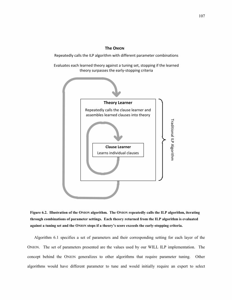
107

Algorithm 6.1 specifies a set of parameters and their corresponding setting for each layer of the

ONION. The set of parameters presented are the values used by our WILL ILP implementation. The

concept behind the ONION generalizes to other algorithms that require parameter tuning. Other

algorithms would have different parameter to tune and would initially require an expert to select

Theory Learner

Clause Learner

Learns individual clauses

Repeatedly calls the clause learner and assembles learned clauses into theory

The ONION

Repeatedly calls the ILP algorithm with different parameter combinations

Evaluates each learned theory against a tuning set, stopping if the learned theory surpasses the early-stopping criteria

Traditio

nal ILP

Algo

rithm

Figure 6.2. Illustration of the ONION algorithm. The ONION repeatedly calls the ILP algorithm, iterating

through combinations of parameter settings. Each theory returned from the ILP algorithm is evaluated

against a tuning set and the ONION stops if a theory’s score exceeds the early-stopping criteria.

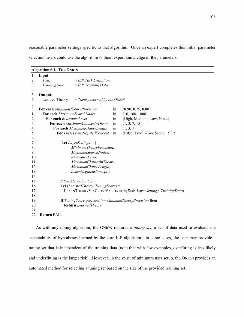
108

reasonable parameter settings specific to that algorithm. Once an expert completes this initial parameter

selection, users could use the algorithm without expert knowledge of the parameters.

As with any tuning algorithm, the ONION requires a tuning set, a set of data used to evaluate the

acceptability of hypotheses learned by the core ILP algorithm. In some cases, the user may provide a

tuning set that is independent of the training data (note that with few examples, overfitting is less likely

and underfitting is the larger risk). However, in the spirit of minimum user setup, the ONION provides an

automated method for selecting a tuning set based on the size of the provided training set.

Algorithm 6.1. THE ONION

1. Input:

2. Task // ILP Task Definition

3. TrainingData // ILP Training Data

4.

5. Output:

6. Learned Theory // Theory learned by the ONION

7.

8. For each MinimumTheoryPrecision in {0.90, 0.75, 0.00}

1. For each MaximumSearchNodes in {10, 100, 1000}

2. For each RelevanceLevel in {High, Medium, Low, None}

3. For each MaximumClausesInTheory in {1, 3, 7, 15}

4. For each MaximumClauseLength in {1, 3, 7}

5. For each LearnNegatedConcept in {False, True} // See Section 6.3.6

6.

7. Let LayerSettings = {

8. MinimumTheoryPrecision,

9. MaximumSearchNodes,

10. RelevanceLevel,

11. MaximumClausesInTheory,

12. MaximumClauseLength,

13. LearnNegatedConcept }

14.

15. // See Algorithm 6.2

16. Let (LearnedTheory, TuningScore) =

17. LEARNTHEORYVIACROSSVALIDATION(Task, LayerSettings, TrainingData)

18.

19. If TuningScore precision >= MinimumTheoryPrecision then

20. Return LearnedTheory

21.

22. Return FAIL

109

Algorithm 6.2 outlines the LEARNTHEORYVIACROSSVALIDATION tuning procedure executed for

each layer of the ONION. Depending on the number of training examples available, the ONION uses one

of two tuning methods. In order to be robust to training sets with few examples (one of the over-arching

goals the ONION), for training sets with less than 25 examples, the ONION uses the training set as the

tuning set, resulting in an overlap of the training and tuning sets. While undesirable, this setup maximize

the amount of training data provided to the ILP algorithm, trading off the likelihood of over-fitting against

the benefit of additional training data. Lines 10-18 of Algorithm 6.2 detail this method of selecting a

tuning set. When the number of training examples exceeds 25, the ONION switches to a cross-validation

(Devijver & Kittler, 1982) approach to tuning, as shown by lines 21-39 of Algorithm 6.2. By default, the

ONION uses a 2-fold cross-validation procedure. The use of cross-validation provides robustness to over-

fitting at the cost of additional learning time and a reduced number of training examples for any single

fold.

6.2 Exploiting Relevance

Although I designed the ONION to be parameter-tuning approach, while designing the algorithm I also

examined allowing the user to provide relevance information about the candidate predicates that ILP uses

to construct hypothesis clauses. Relevance indicates the user’s believe that a predicate will be in the

learned concept, allowing a user to exploit their knowledge of the domain. This form of domain

knowledge does not require detailed understanding of the underlying ILP algorithm and thus provides an

excellent method for the user to provide additional hints to the ILP algorithm. Automated methods, such

as our advice-handling process detailed in Chapter 4, also produce this relevance information based on

teacher-provided instruction.

110

Table 6.1 lists the relevance strengths supported by our WILL ILP implementation. The ONION

provides relevance support using the same methodology as other parameters, by iteratively expanding the

search space, initially including only the most relevant predicate and later considering less relevant

predicates. When the ONION considers weaker relevance levels, it also considers all more relevant target

Algorithm 6.2. LEARNTHEORYVIACROSSVALIDATION

1. Input:

2. Task // ILP Task Definition

3. LayerSettings // Settings for the current layer of the ONION

4. TrainingData // Complete set of training data

5.

6. Outputs:

7. LearnedTheory // Best learned theory

8. TuningSet score // Score of the best learned theory on tuning test

9.

10. If | TrainingData | < 25 then

11. // Low example count tuning procedure – no cross-validation

12. Let CVTrainingData = TrainingData

13. Let CVTuningData = TrainingData

14.

15. Let LearnedTheory = RUNILP(Task, CVTrainingData)

16.

17. Let TuningScore = score of the LearnedTheory evaluated on CVTuningData

18.

19. Return (LearnedTheory, TuningScore)

20.

21. else

22. // Cross-validation tuning procedure

23. Let BestLearnedTheory = ∅

24. Let BestTuningScore = 0

25.

26. for n in 1 to 3

27. Let CVTuningData = nth third of TrainingData

28. Let CVTrainingData = remaining TrainingData

29.

30. Let LearnedTheory = RUNILPALGORITHM(Task, CVTrainingData)

31.

32. Let TuningScore = score of the LearnedTheory evaluated on CVTuningData

33.

34. If TuningScore > BestTuningScore then

35. Let BestTuningScore = TuningScore

36. Let BestLearnedTheory = LearnedTheory

37.

38. Return (BestLearnedTheory , BestTuningScore)

111

predicates, i.e., when considering the RELEVANT relevance strength, the ONION also includes all the

VERYSTRONGLYRELEVANT, VERYSTRONGLYRELEVANTNEG, POSSIBLEANSWER, and

POSSIBLEANSWERNEG relevant predicates. Although Table 6.1 specifies 14 separate relevance strengths,

to reduce the number of ONION layers, the ONION divides the 14 strengths into 4 groups, as shown in the

3rd

column of Table 6.1.

6.3 Parameters to Tune

The following section details the specific parameters used by our WILL ILP system. Algorithm 6.1

shows the primary parameters tuned by the ONION. From these, the ONION derives several secondary

parameters, as shown in Table 6.2. We also detail both the primary and secondary parameters in this

section.

Table 6.1. Relevance Strengths and associated meanings, listed in order of their relative strengths.

Relevance

Strength

Meaning Onion

Layer

POSSIBLEANWER

POSSIBLEANWERNEG†

Target predicate alone may be the actual concept. High

VERYSTRONGLYRELEVANT

VERYSTRONGLYRELEVANTNEG†

Target concept highly likely to use target predicate. Medium

RELEVANT

RELEVANTNEG†

Target concept likely to use target predicate. Low

ISMENTIONEDINSIDEADVICE Advice used this target predicate. None

WEAKLYRELEVANT

WEAKLYRELEVANTNEG†

Target predicate may be relevant, but not likely. None

ISOBSERVEDFEATURE The target predicate was observed in some way somewhere in the

domain (i.e., via the process used to collect the data or via

watching some human teacher specify advice), but the relevance

strength is unknown.

None

NEUTRAL User has no knowledge about the relevance of target predicate.

Default relevance strength.

None

WEAKLYIRRELEVANT Target predicate is somewhat unlikely to be relevant. None

IRRELEVANT Target predicate is unlikely to be relevant. Skipped

STRONGLYIRRELEVANT Target predicate is very unlikely to be relevant. Skipped

† The NEG relevance strengths perform the same functions as their corresponding non-NEG relevance strength.

However, the NEG version indicates that the knowledge somehow derives from the negative examples or

negative advice.

112

6.3.1 MinimumTheoryPrecision Parameter

The MinimumTheoryPrecision dictates the minimum precision required by the ONION to accept a

learned theory as the final answer. Initially, the ONION attempts aggressively high precision values,

slowly iterating through less stringent precision criteria. This helps prevent the ONION from settling on a

marginal answer when better ones might be found through additional search.

For any given layer, the ONION adjusts the actual MinimumTheoryPrecision used during learning

according to the following criteria:

If MinimumTheoryPrecision < the best possible mEstimate adjusted precision

then MinimumTheoryPrecision = best possible mEstimate adjusted precision.

If MinimumTheoryPrecision < best possible precision by predicting the major class

then MinimumTheoryPrecision = best possible major class precision.

These criteria guarantee that learned theories can achieve the MinimumTheoryPrecision and that the

learned theory outperforms the trivial theory predicting the majority class.

The F1EarlyStoppingScore is directly calculated from the MinimumTheoryPrecision parameter

setting. After each layer completes, the resulting theory is scored on the tuning set, generating an F1

score. If that F1 score is greater than the F1EarlyStoppingScore, the Onion terminates, returning the

learned theory. An F1 score is the harmonic mean of the precision and recall scores. When calculating

the F1EarlyStoppingScore, we assume that the desired recall of the final theory is equal to the

Table 6.2. Primary and secondary parameters tuned through the ONION.

Parameter Type Description

MinimumTheoryPrecision Primary Minimum precision of final learned theory

F1EarlyStoppingScore Secondary Minimum F1 score to terminate the Onion

MaximumSearchNodes Primary Number of clauses to search in the inner ILP loop before stopping

MaximumClauseLength Primary Maximum literals in any single clause learned by inner ILP loop

MaximumClausesInTheory Primary Maximum clauses in any single learned theory

MinimumPrecisionPerClause Secondary Minimum precision of any single clause learned by inner ILP loop

MinimumRecallPerClause Secondary Minimum recall of any single clause learned by inner ILP loop

LearnNegatedConcept Primary Indicates ILP should search for the negated target concept

113

MinimumTheoryPrecision parameter setting. Given this assumption, F1EarlyStoppingScore turns out to

equal the MinimumTheoryPrecision.

6.3.2 MaximumSearchNodes Parameter

The MaximumSearchNodes parameter controls how many search nodes the ILP algorithm creates

before it abandons the search and stops the ILP clause learner (i.e., the inner most ILP search process).

Early ONION layers constrain the search dramatically, while later allowing for much more extensive

search of the space.

6.3.3 RelevanceStrength Parameter

As discussed earlier, in Section 3.3, the RelevanceStrength affects which predicates composed the

search space during of any given layer. We use parameters of High, Medium, Low, and None during the

search. However, if the user provides no relevance information (and none is generated automatically),

one or more of the relevance levels may result in the same set of included predicates and thus the same

hypothesis space. For instance, if all predicates have a relevance level of NEUTRAL, they would all be

first explored in the None layer of the ONION, thus there would be no point in searching the High,

Medium, and Low layers. When this occurs, the ONION prunes the duplicate or irrelevant layers, skipping

them completely.

6.3.4 MaximumClausesInTheory Parameter

Some concepts are naturally disjunctive. A single Horn clause does not allow the expression of

disjunctive concepts. To express disjunctive concepts, a theory must use multiple clauses. The

MaximumClausesInTheory parameter controls how many Horn clauses a learned theory may contain.

Initially, the ONION attempts to find non-disjunctive theories consisting of only a single clause. If this

114

approach fails to produce a theory, the ONION allows theories with multiple clauses, increasing the

number of clauses allowed in later layers.

When considering theories with multiple clauses, we expect any give clause of the theory to cover

only a subset of the positive examples. For example, if we consider the disjunctive concept (

), we might learn three clauses: , , and . Any given clause may cover, say, only a third

of the positive examples. However, the overall theory may cover all of the positive examples. At the

same time given that any single clause must cover fewer examples, we expect the individual clauses to be

more precise.

To account for this, the ONION introduces two additional derived parameters:

MinimumPrecisionPerClause and MinimumRecallPerClause, defined as:

(

)

(6.1)

(6.2)

Figure 6.3 depicts the relationship between these two values. Higher MaximumClausesInTheory

parameter settings greatly reduce the recall required for any single clause. Although not as evident in the

figure, the MinimumPrecisionPerClause parameter setting increases as the MaximumClausesInTheory

increases.

6.3.5 MaximumClauseLength Parameter

The MaximumClauseLength controls the number of literals allowed in the body of the any single

learned clause. The size of the hypothesis space increases exponetially with the MaximumClauseLength.

Thus, we constrain the early ONION layers to clauses containing only a single literal, again relaxing this

requirement in later layers. The RelevanceStrength parameter setting affects the values tried for the

MaximumClauseLength parameter. When the RelevanceStrength parameter is set to High, layers

115

exploring MaximumClauseLength = 1 exist. However, when RelevanceStrength is not High, the Onion

skips this set of layers.

Although a single literal may seem overly restrictive, WILL does not count accessors literals when

determining the clause length. Our logical representation does not support logical functions. Accessors

literals essentially implement logical functions through a literal, resolving to a single function value for

any given input. For instance, the x_position predicate may access the x position of some object allowing

the use of that value later in the clause. Typically, accessor function values provide no directly

discriminator power by themselves, i.e., they provide no gain in the score of a hypothesis clause.

However, when considered with the literals that use the function values, the accessor literals often

contribute to a gain in the score. Because of this, WILL explores extensions to the hypothesis clauses via

accessors despite their immediately lack of gain and considers these accessor “free,” not counting them as

part of the clause length.

Figure 6.3. Adjustments to Per-Clauses Minimum Recall. The minimum recall of a single component

clause of a learned theory scales linearly with the minimum per-clause precision. Additionally, as the

maximum number of allowed clauses in a theory increases, the minimum required recall is reduced.

0.50

0.55

0.60

0.65

0.70

0.75

0.80

0.85

0.90

0.95

1.00

0.00 0.20 0.40 0.60 0.80 1.00

Min

imu

m P

reci

sio

n P

er

Cla

use

Minimum Recall Per Clause

1

3

7

15

Maximum Clauses In

Theory

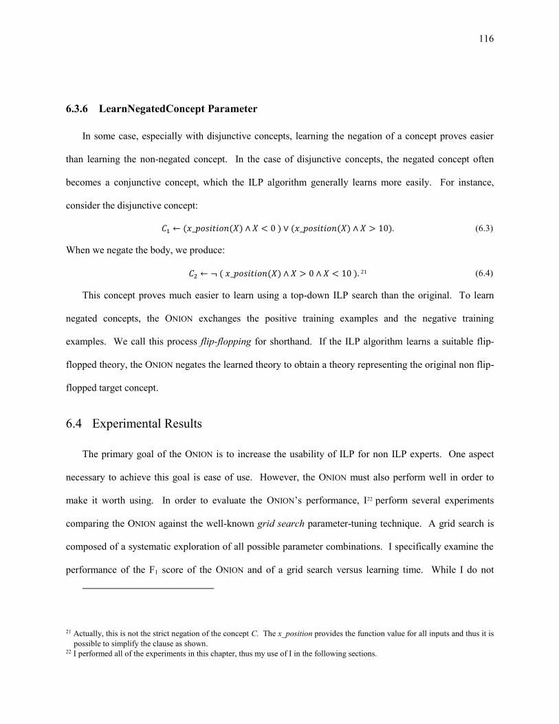
116

6.3.6 LearnNegatedConcept Parameter

In some case, especially with disjunctive concepts, learning the negation of a concept proves easier

than learning the non-negated concept. In the case of disjunctive concepts, the negated concept often

becomes a conjunctive concept, which the ILP algorithm generally learns more easily. For instance,

consider the disjunctive concept:

( ( ) ) ( ( ) ) (6.3)

When we negate the body, we produce:

( ( ) ) 21 (6.4)

This concept proves much easier to learn using a top-down ILP search than the original. To learn

negated concepts, the ONION exchanges the positive training examples and the negative training

examples. We call this process flip-flopping for shorthand. If the ILP algorithm learns a suitable flip-

flopped theory, the ONION negates the learned theory to obtain a theory representing the original non flip-

flopped target concept.


The primary goal of the ONION is to increase the usability of ILP for non ILP experts. One aspect

necessary to achieve this goal is ease of use. However, the ONION must also perform well in order to

make it worth using. In order to evaluate the ONION’s performance, I22 perform several experiments

comparing the ONION against the well-known grid search parameter-tuning technique. A grid search is

composed of a systematic exploration of all possible parameter combinations. I specifically examine the

performance of the F1 score of the ONION and of a grid search versus learning time. While I do not

21 Actually, this is not the strict negation of the concept C. The x_position provides the function value for all inputs and thus it is

possible to simplify the clause as shown. 22 I performed all of the experiments in this chapter, thus my use of I in the following sections.

117

expect the ONION to outperform a grid search in all situations, its performance should not be significantly

worse. I use three separate ILP tasks during these experiments: Advised-By (see Section 3.3.1),

Carcinogenesis (see Section 3.3.2), and Mutagenesis (see Section 3.3.3). All three are standard ILP

testbeds used previously by other researchers.

6.4.1 Methodology

For each of the three experiment tasks, I run both the ONION algorithm and I run a complete grid

search over all possible combinations of the parameters settings listed in Table 6.3, resulting in 27

separate parameter setting combinations. These are the default ONION parameter settings with a few

exceptions. While the ONION would normally also attempt a MaximumClauseLength of 15, I disabled

that setting for these experiments. The ONION attempts that length for completeness, in case a concept is

particularly complicated. However, I felt it was unfair to the grid search to attempt that setting given the

low likelihood it would be necessary. This is the type of tuning decision that ILP experts regularly make,

even when using a grid-search approach. Additionally, since none of the tasks have associated advice, all

literal determinations have a NEUTRAL relevance strength. The Onion automatically skips all the ONION

layers pertaining to relevance strengths other than NEUTRAL. Finally, I only explore the non-negated

concept learning, as these tasks have a skew between positive and negatives reducing the effectiveness of

learning negated concepts.

Table 6.3. Parameter settings tried during grid search and ONION experiments.

ILP Parameter Possible Settings

Minimum Theory Precision 0.85, 0.70, 0.00

Maximum Search Nodes 1000

Relevance Strength NEUTRAL

Maximum Clauses in Theory 1, 3, 7

Maximum Clause Length 3, 5, 7

Learn Negated Concept False

118

For each experiment, I run N folds, as specified in Table 6.4. For the Advised-By and Carcinogenesis

tasks, I use (N-1) sub-folds to perform tuning as depicted in Figure 6.4. The experiments using the

ONION perform internal tuning in a similar manner. Since the Mutagenesis data set is small, I use the

training set also as the tuning set.

... Chunk NChunk 1

Chunk N-1

Chunk N

Chunk 1

Fold N

......

Chunk N

Chunk 1

Chunk 2

...

Fold 1Testset

Fold 1Non-Testset

Fold NTestset

Fold NNon-Testset

Chunk N-2

Chunk N-1

Chunk 1

......Chunk

NChunk

1Chunk

2...

Fold 1/1 Tuneset

Fold 1/1Trainset

Fold N/(N-1)Tuneset

Fold N/(N-1)Non-Testset

N-1 Subfolds of Fold 1 Non-Testset

All Example

Fold 1

Figure 6.4. Training, tuning, and testing folds for grid-search experiments.

Table 6.4. Dataset sizes for ONION versus grid-search experiments.

Task Total # of Positive Examples Total # of Negative Examples Testing Folds

Advised-By 115 1675 4

Carcinogenesis 182 148 3

Mutagenesis 13 29 2

119

The ONION algorithm generates only a single F1 score per fold, thus for each task we get N ONION

algorithm data points, where N is the number of testing folds for the task. For the grid search, I generate a

learning curve by simulating multiple grid searches of various sizes, sub-sampling from all grid-search

results. Algorithm 6.3 GENERATEGRIDSEARCHLEARNINGCURVE repeatedly calls Algorithm 6.4

GENERATEGRIDSEARCHSAMPLESCORE to generate samples of size k, where k varies from 1 to the total

number of parameter combinations. GENERATEGRIDSEARCHSAMPLESCORE returns a pair of values

representing the total time taken during a simulated grid of size k and the best testing score determined by

finding the best sub-fold testing score based upon sub-fold tuning scores.

GENERATEGRIDSEARCHLEARNINGCURVE is run separately for each testing fold. Thus, N separate

learning curves are created, one for each fold.

Algorithm 6.3. GENERATEGRIDSEARCHLEARNINGCURVE

1. Input:

1. // Map contains a key entry for each parameter setting combination mapping

2. // to a set of (N-1) sub-fold results (i.e., N-1 results per setting combinations.)

3. Map M of <settings> to set of <sub-fold, time, F1TuningScore, F1TestingScore>

4.

5. Output:

6. Set <time, F1TestingScore> // Set composing the learning curve of time versus F1 score

7.

8. Let S =

9. For sampleSize in 1 to <# of parameter combinations>

10. For repetitions in 1 to 20

11. Let <time, F1TestScore> = GENERATEGRIDSEARCHSAMPLESCORE(M, sampleSize)

12. Let S = S <time, F1TestScore>

13.

14. Return S

120

6.4.2 Results

Figure 6.5, Figure 6.6, and Figure 6.7 show the experimental results for the Advised-By,

Carcinogenesis, and Mutagenesis experiment. Each of individual points represent the F1 score of a

Algorithm 6.4. GENERATEGRIDSEARCHSAMPLESCORE

1. Input:

2. // Map contains a key entry for each parameter setting combination mapping

3. // to a set of (N-1) sub-fold results (i.e., N-1 results per setting combinations.)

4. Map M of <settings> to set of <sub-fold, time, F1TuningScore, F1TestingScore>

5.

6. sampleSize // Number of parameter settings to sample

7.

8. Output:

9.

10. <time, F1TestScore> // Total time and best testing score

11.

12. Let totalTime = 0

13. Let bestOverallTestScore = 0

14. Let bestOverallTuneScore = 0

15.

16. For sample in 1 to sampleSize

17. Randomly select key K from M, without replacement

18. Let R = M{K} // Set of sub-fold results for settings K

19.

20. Let bestSubfoldTuneScore = 0

21. Let bestSubfoldTestScore = 0

22. Let subfoldTime = 0

23.

24. For aResult in R // Select best tuning score from sub-folds and record time and test score

25. If aResult.F1TuningScore > subfoldTungScore then

26. Let bestSubfoldTuneScore = aResult.F1TuningScore

27. Let bestSubfoldTestScore = aResult.F1TestingScore

28.

29. // Update total time to include all time spent during sub-fold learning

30. Let totalTime = aResult.time

31.

32. // Update the best overall score based on the best sub-fold score

33. If bestSubfoldTuneScore > bestOverallTuneScore then

34. Let bestOverallTuneScore = bestSubfoldTuneScore

35. Let bestOverallTestScore = bestSubfoldTestScore

36.

37. Return (totalTime, bestOverallTestScore)

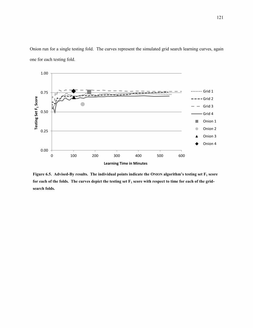
121

Onion run for a single testing fold. The curves represent the simulated grid search learning curves, again

one for each testing fold.

Figure 6.5. Advised-By results. The individual points indicate the ONION algorithm’s testing set F1 score

for each of the folds. The curves depict the testing set F1 score with respect to time for each of the grid-

search folds.

0.00

0.25

0.50

0.75

1.00

0 100 200 300 400 500 600

Te

stin

g Se

t F 1

Sco

re

Learning Time in Minutes

Grid 1

Grid 2

Grid 3

Grid 4

Onion 1

Onion 2

Onion 3

Onion 4

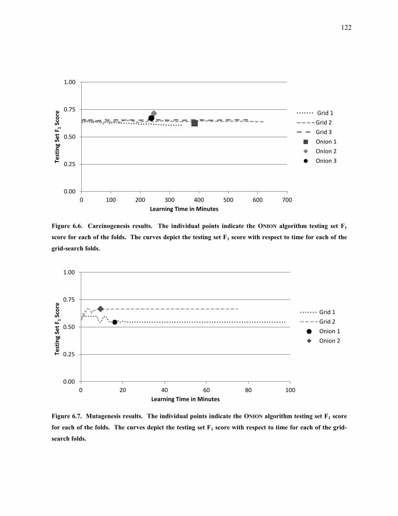
122

Figure 6.7. Mutagenesis results. The individual points indicate the ONION algorithm testing set F1 score

for each of the folds. The curves depict the testing set F1 score with respect to time for each of the grid-

search folds.

0.00

0.25

0.50

0.75

1.00

0 20 40 60 80 100

Test

ing

Set

F 1 S

core


Grid 1

Grid 2

Onion 1

Onion 2

Figure 6.6. Carcinogenesis results. The individual points indicate the ONION algorithm testing set F1

score for each of the folds. The curves depict the testing set F1 score with respect to time for each of the

grid-search folds.

0.00

0.25

0.50

0.75

1.00

0 100 200 300 400 500 600 700

Test

ing

Set

F 1 S

core


Grid 1

Grid 2

Grid 3

Onion 1

Onion 2

Onion 3

123

In the case of the Advised-By task, on three of the four folds, the ONION performs equally as well as

the grid search, although the grid search runs reach their asymptotes in less time. However, the learning

curves for the grid search are simulated. In practice, a grid search performs all parameter setting

combinations and actually takes the maximum time shown in the curves.

The ONION fares better on the Carcinogenesis tasks. In two of the three folds, it actually outperforms

the grid search. By examining the individual grid search runs, I determined that during the grid search

there were many parameter combinations that performed well on their tuning sets but poorly on their

testing sets. While the ONION would have eventually reached these parameter combinations, it stopped

prior to encountering them, resulting in better performance. This behavior is a form of over-fitting

avoided through early stopping by the ONION and is one of the advantages of the ONION.

Finally, in the Mutagenesis task, the ONION and grid search perform similarly. In the first fold, over-

fitting is again evident. In this case, both the ONION and the grid search over-fit the data. Given the small

number of training examples available for the Mutagenesis task this is not unexpected as there are not

enough examples to create separate training and tuning sets.

6.4.3 Discussion

As the experiments show, the ONION does not always outperform a grid search. This is expected, as

both approaches search the same hypothesis spaces and will learn the same theory for any given

parameter combination. However, it is important to note that while the performance of the ONION might

be similar to the grid search, the ONION provides stopping criteria that substantially reduce the runtime

compared to a complete grid search. While the simulated grid search appears to outperform the ONION in

terms of runtime, in practice without a way to (a) order the search spaces and (b) determine when to stop

early, a grid search must examine all parameter combinations and thus the actual runtime is maximum

time shown in the graphs.

124

6.5 Why the ONION is Needed

Changes in an ILP parameter setting often produces non-predictable change in performance, i.e.,

smoothly changing a single parameter setting over a range of values does not result in a smooth change in

performance. Additionally, the interaction between multiple parameter settings often varies in

unpredictable ways. This effect is important because it limits the use of more principled and efficient

parameter-tuning approaches, such as gradient-descent methods (Snyman, 2005) or simulated annealing

(Cerny, 1985). In order to demonstrate this effect, I examine how several individual parameter settings

and combinations of parameter settings affect ILP performance.

6.5.1 Methodology

To demonstrate the non-smooth effect of changes in parameter settings, I look at the results data from

Experiment C in Section 4.2, which examines of labeling errors on ILP performance for tasks in the

Bootstrap Learning domain (see Section 3.1). I use this data set as it provide more diversity than the

experiments in Section 6.4, using 14 separate tasks and introducing a controlled amount of example noise.

Additional, since Experiment C includes advice, its results allow the comparison of advice and no-advice

learning scenarios.

Experiment C provides results for both 24 training examples (12 positive and 12 negative) and 100

training examples (50 positive and 50 negatives). I use only the results that use 100 examples. While

Experiment C varies the example noise from 0% to 45%, I use only the data ranging from 0% to 15%

example noise, as this more realistically represents the levels of example noise one might encounter in

real-world tasks. All of the results below aggregate the results from all Experiment C tasks and examine

the effect of varying one or more parameters. All of the source data from Experiment C use the ONION

during learning.

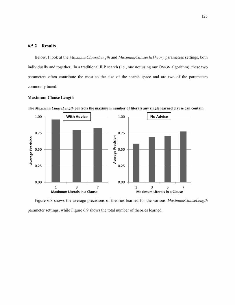
125

6.5.2 Results

Below, I look at the MaximumClauseLength and MaximumClausesInTheory parameters settings, both

individually and together. In a traditional ILP search (i.e., one not using our ONION algorithm), these two

parameters often contribute the most to the size of the search space and are two of the parameters

commonly tuned.

Maximum Clause Length

The MaximumClauseLength controls the maximum number of literals any single learned clause can contain.

Figure 6.8 shows the average precisions of theories learned for the various MaximumClauseLength

parameter settings, while Figure 6.9 shows the total number of theories learned.

0.00

0.25

0.50

0.75

1.00

1 3 7

Ave

rage

Pre

cisi

on

Maximum Literals in a Clause

With Advice

0.00

0.25

0.50

0.75

1.00

1 3 5 7

Ave

rage

Pre

cisi

on


No Advice

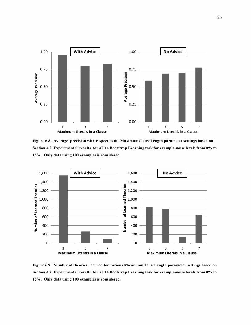
126

Figure 6.9. Number of theories learned for various MaximumClauseLength parameter settings based on

Section 4.2, Experiment C results for all 14 Bootstrap Learning task for example-noise levels from 0% to

15%. Only data using 100 examples is considered.

0

200

400

600

800

1,000

1,200

1,400

1,600

1 3 7

Nu

mb

er

of

Lear

ne

d T

he

ori

es


With Advice

0

200

400

600

800

1,000

1,200

1,400

1,600

1 3 5 7

Nu

mb

er

of

Lear

ne

d T

he

ori

es


No Advice

Figure 6.8. Average precision with respect to the MaximumClauseLength parameter settings based on



0.00

0.25

0.50

0.75

1.00

1 3 7

Ave

rage

Pre

cisi

on


With Advice

0.00

0.25

0.50

0.75

1.00

1 3 5 7A

vera

ge P

reci

sio

n


No Advice

127

When using advice, there is little variation in the precision across the different parameter settings.

For advice, the number of theories learned when MaximumClauseLength = 1 outnumbers the others; this

is expected and shows that the ONION is taking advantage of the advice. For no-advice runs, there is an

upward trend in average precision as MaximumClauseLength increases. In order to examine this trend

further, Figure 6.10 shows a comparison of the average precision for 0% and 15% example-noise levels

separately (previous figures averaged over all example noise results.) As can be seen, for 0% noise the

increase in average precision is much less pronounced while the results with noisy training data follow a

similar pattern as the no-advice results from This demonstrates that, while some trends occur with respect

to MaximumClauseLength, those trends only occur in limited circumstances.

MaximumClausesInTheory

The MaximumClausesInTheory controls the maximum number of individual clauses a learned theory

may contain, which is necessary in order to represent disjunctive concepts. Figure 6.11 shows the

Figure 6.10. Average precision with respect to the MaximumClauseLength for 0.0 and 0.15 example

noise levels. Average of precision from on Section 4.2, Experiment C results for all 14 Bootstrap Learning

tasks.

0.00

0.25

0.50

0.75

1.00

1 3 5 7

Ave

rage

Pre

cisi

on


0% Noise - No Advice

0.00

0.25

0.50

0.75

1.00

1 3 7

Ave

rage

Pre

cisi

on


15% Noise - No Advice

128

average precisions of theories learned for the various MaximumClausesInTheory parameter settings, while

Figure 6.12 shows the total number of theories learned.

The results for average precision with respect to MaximumClausesInTheory show less of a trend than

the previous MaximumClauseLength results, both for advice and for no-advice. For advice there is a large

number of learned theories with only a single clause in the theory, while the number of no-advice theories

is distributed evenly between the different parameter settings. This difference is easily explained by the

presence of the background knowledge generated from advice. In tasks where a disjunctive learned

theory is required, some of the background knowledge introduced through the advice takes the form of

disjunctive mega-clauses. Without advice, disjunctive concepts require a MaximumClauseLength greater

than one.

Figure 6.11. Average precision with respect to the MaximumClausesInTheory parameter settings based on



0.00

0.10

0.20

0.30

0.40

0.50

0.60

0.70

0.80

0.90

1.00

1 3 7

Ave

rage

Pre

cisi

on

Maximum Clauses in Theory

With Advice

0.00

0.10

0.20

0.30

0.40

0.50

0.60

0.70

0.80

0.90

1.00

1 3 7

Ave

rage

Pre

cisi

on

Maximum Clauses in Theory

No Advice

129

MaximumClauseLength and MaximumClausesInTheory Interaction

Above, the average precision of the learned theories showed weak trends, especially with respect to

the MaximumClauseLength parameter without advice. From this, one might conclude that one could tune

the MaximumClauseLength parameter using optimization techniques mentioned earlier. However, this

does not take into account the interactions between the various ILP parameters. In order to examine this

aspect, Figure 6.13 (with advice) & Figure 6.14 (no advice) presents the average precision and Figure

6.15 (with advice) & Figure 6.16 (no advice) provides the distribution of learned theories for all possible

parameter combinations of MaximumClauseLength and MaximumClausesInTheory together.

Figure 6.12. Number of theories learned for various MaximumClausesInTheory parameter settings based

on Section 4.2, Experiment C results for all 14 Bootstrap Learning task for example-noise levels from 0%

to 15%. Only data using 100 examples is considered.

0

200

400

600

800

1000

1200

1400

1600

1 3 7

Nu

mb

er

of

Lear

ne

d T

he

ori

es

Maximum Clauses in a Theory

With Advice

0

200

400

600

800

1000

1200

1400

1600

1 3 7

Nu

mb

er

of

Lear

ne

d T

he

ori

es

Maximum Clauses in a Theory

No Advice

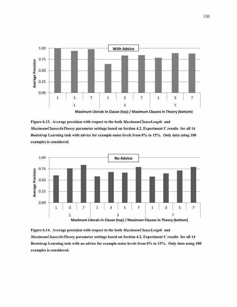
130

Figure 6.14. Average precision with respect to the both MaximumClauseLength and

MaximumClausesInTheory parameter settings based on Section 4.2, Experiment C results for all 14

Bootstrap Learning task with no advice for example-noise levels from 0% to 15%. Only data using 100

examples is considered.

0.00

0.25

0.50

0.75

1.00

1 3 7 1 3 5 7 1 3 5 7

1 3 7

Ave

rage

Pre

cisi

on

Maximum Literals In Clause (top) / Maximum Clauses in Theory (bottom)

No Advice

Figure 6.13. Average precision with respect to the both MaximumClauseLength and


Bootstrap Learning task with advice for example-noise levels from 0% to 15%. Only data using 100


0.00

0.25

0.50

0.75

1.00

1 3 7 1 3 7 1 3 7

1 3 7

Ave

rage

Pre

cisi

on


With Advice

131

When we consider MaximumClauseLength and MaximumClausesInTheory together, all obvious

trends disappear. The Onion still learns a large number of theories at the (MaximumClauseLength = 1,

Figure 6.16. Number of theories learned for various both MaximumClauseLength and


Bootstrap Learning task with no advice for example-noise levels from 0% to 15%. Only data using 100


0

100

200

300

400

500

600

1 3 7 1 3 5 7 1 3 5 7

1 3 7

Nu

mb

er

of

The

ori

es

Lear

ne

d


No Advice

Figure 6.15. Number of theories learned for various both MaximumClauseLength and


Bootstrap Learning task with advice for example-noise levels from 0% to 15%. Only data using 100


0

200

400

600

800

1,000

1,200

1,400

1 3 7 1 3 7 1 3 7

1 3 7

Nu

mb

er

of

The

ori

es

Lear

ne

d


With Advice

132

MaximumClausesInTheory = 1) parameter combination when using advice, but this is expected for the

same reasons we saw this effect above. This further demonstrates the non-smooth performance with

respect to the parameter settings.

6.5.3 Discussion

I predicated much of the necessity of the ONION on the difficulty of tuning ILP parameters. If the ILP

parameters could be tuned through an optimization method, it would be more effective to use such

methods. However, as demonstrated above, the performance of ILP does not vary predictively with

respect to the parameters and a tuning process like the ONION must be used.

An automated tuning process is especially important for non ILP expert users, as they are unlikely to

know even where to focus the search to produce good performance. An ILP expert at least may

understand the parameter settings likely to produce good performance, guided by both an understanding

of the parameters and previous experience. However, even in this case, the above results indicate that it is

difficult to predict what parameter combinations will result in good performance.

6.6 Related Work

Automatic parameter selection for machine-learning methods has been explored earlier (Kohavi,

John, & Prieditis, 1995), where the goal is to use the expected error for each parameter setting to guide

the selection of the parameters for decision trees. Lavrac et al. (1999) proposed a feature selection

framework for ILP that worked well in propositional learning and special cases of relational learning.

This was later extended by Alphonse and Matwin (2002) using powerful statistical feature-selection

techniques to control the dimensionality of the search space. The key idea in their work is to reduce ILP

examples to non-recursive clauses by removing irrelevant literals. Muggleton (1995) theoretically shows

that as the number of predicates in the background theory increases, the size of the search space of an ILP

133

system can increase greatly. This necessitates the intervention of an ILP expert who can reduce the

search space. In such a context, relevance information and automated parameter tuning becomes crucial.


The main purpose of the ONION is to provide an effective parameter-tuning method, accessible to

users without ILP expertise via an iterative-deepening style search of possible parameter combinations.

This is critical both due to the number of parameters and ILP’s high sensitivity to parameter settings.

Through the mechanism of early-stopping criteria, the ONION reduces over-fitting while improving

efficiency compared to a grid search. Additionally, the ONION’s support of relevance information

provides a simple way for users to provide knowledge about the importance of predicates. The support of

relevance information also facilitates the advice giving algorithm presented in Chapter 4, as well as

allowing concepts to be learned with fewer examples.

One limitation of the ONION is its serial nature; the ONION searches layer sequentially until an

acceptable theory is found. While this property is advantageous in some respects, the ONION is not able

to take advantage of multiple processors. This is one area in which a grid search has a clear advantage.

One future research direction would be to parallelize the ONION. In the simplest approach, this might

entail running multiple layers at once while still evaluating the results sequential order. Another future

direction might be to consider more parameter combinations. This has the side effect of increasing the

number of layers and thus increasing the search time, which is undesirable. Approaches such as randomly

selecting layers to search according to some weighted distribution might allow a wider range of parameter

combinations to be considered while retaining many of the efficiency and ease of use benefits of the

ONION.

134

7 Additional Explorations – Building Relational World Models

Prior to the work presented earlier in this document, I explored several tangential directions in the

field of relational reinforcement learning. This prior work used inductive logic programming (ILP)

extensively and provided much of the motivation for the main body of work, specifically concerning

automatic generation of background knowledge and improving the ease of use for ILP.

In this chapter, I explore the automatic generation of background knowledge guided by the

information produced during the course of solving a reinforcement-learning task. The end goal of this

research was to generate a relational model of the reinforcement-learning task that could be used to solve

the task faster than traditional Q-learning approaches. This approach to solving the reinforcement-

learning task falls under the model-based class of reinforcement-learning approaches, as discussed in

Section 2.3.3. Specifically, I look at Markov decision process (MDP) abstraction, where the MDP

represents the underlying state-transition and reward model of a reinforcement-learning task, in scenarios

where the underlying parameters of the MDP (i.e., the state-transition function and reward function) are

unknown.

Markov decision-process abstraction is a learning method where the original MDP (whose parameters

are possibly unknown to the learner) is modeled via a second abstract MDP, the A-MDP23, created during

learning. For instance, the left half of Figure 7.1 depicts a state-transition function for a single action for

small discrete MDP. The right half of the figure shows one possible abstract A-MDP. In order to be

useful for learning, the learner attempts to devise an A-MDP that maintains some degree of congruency

with the original.

23 The nomenclature A-MDP is not standard reinforcement learning or MDP terminology. I use it throughout this chapter to

clarify the difference between the underlying MDP and the abstract one learned via my algorithm.

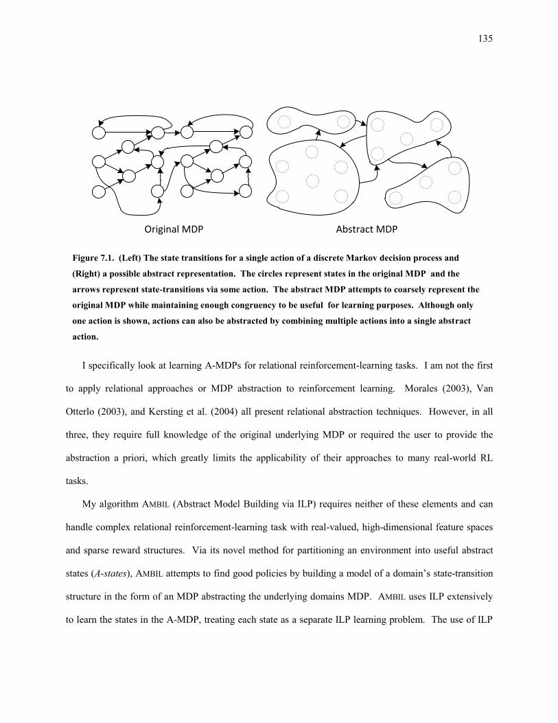
135

I specifically look at learning A-MDPs for relational reinforcement-learning tasks. I am not the first

to apply relational approaches or MDP abstraction to reinforcement learning. Morales (2003), Van

Otterlo (2003), and Kersting et al. (2004) all present relational abstraction techniques. However, in all

three, they require full knowledge of the original underlying MDP or required the user to provide the

abstraction a priori, which greatly limits the applicability of their approaches to many real-world RL

tasks.

My algorithm AMBIL (Abstract Model Building via ILP) requires neither of these elements and can

handle complex relational reinforcement-learning task with real-valued, high-dimensional feature spaces

and sparse reward structures. Via its novel method for partitioning an environment into useful abstract

states (A-states), AMBIL attempts to find good policies by building a model of a domain’s state-transition

structure in the form of an MDP abstracting the underlying domains MDP. AMBIL uses ILP extensively

to learn the states in the A-MDP, treating each state as a separate ILP learning problem. The use of ILP

Original MDP Abstract MDP

Figure 7.1. (Left) The state transitions for a single action of a discrete Markov decision process and

(Right) a possible abstract representation. The circles represent states in the original MDP and the

arrows represent state-transitions via some action. The abstract MDP attempts to coarsely represent the

original MDP while maintaining enough congruency to be useful for learning purposes. Although only

one action is shown, actions can also be abstracted by combining multiple actions into a single abstract

action.

136

techniques provides power and generality to our models that would otherwise be unattainable with other

approaches.

In complex domains, generalization by function approximators, often used by traditional Q-learning

(Sutton & Barto, 1998), can pose significant difficulties and typically requires a large amount of training

data. AMBIL attempts to improve generalization by focusing on the state transitions seen in the training

data. AMBIL uses ILP to partition the state space and, since these partitions are based directly upon the

state transitions of actions, may generalize the examples more effectively. AMBIL exploits the relational

aspects of RL domains; similar domain actions can be abstracted and learned together rather than

individually. AMBIL also abstracts objects in the domain, learning rules that apply to whole classes of

objects.

The partitions learned by AMBIL form a relational abstract MDP, with the transition and reward

function estimated from previously observed data. Existing techniques, such as value-iteration (Sutton &

Barto, 1998), provide estimates of the expected reward for each A-MDP state. AMBIL’s A-MDP both

determines the policy and provides an explicit, easy-to-analyze representation of the domain.

I present empirical results in a synthetic domain and in the challenging Breakaway subtask of the

RoboCup soccer domain (Maclin, Shavlik, Torrey, Walker, & Wild, 2005), demonstrating faster learning

and higher asymptotes at convergence than traditional Q-learning reinforcement-learning algorithms.

7.1 Building World Models

AMBIL partitions the state space and creates an A-MDP from the partitions. First-order logical rules

define the portion of state space each partition covers. The A-MDP in turn leads to a policy intended to

maximize the rewards received. AMBIL then exploits this policy to collect more examples from the RL

task. AMBIL iterates between building models and utilizing those models in the task. Figure 7.2 depicts a

sample MDP produced by AMBIL. The following sections explain the model-building process.

137

7.1.1 Terminology

AMBIL operates on a collection of examples containing sequences of {state, action, reward} tuples

from the RL task we are attempting to solve. I will refer to these tuples as instance in the space of E-

states. As we partition the E-state space, the individual partitions become A-states in the learned A-MDP.

Similarly, I refer to the non-abstracted MDP underlying the RL task as the E-MDP24. Additionally, when

specifying variables I will use uppercase letters for A-states and lowercase letters for E-states. E.g., an A-

state might be S while an E-state might be s. The E-MDP and A-MDP use the same set of actions as the

original MDP, thus this distinction is not necessary for action variables.

AMBIL bases its partitioning upon preimages of the current, partially built A-MDP. The preimage of

an A-state S for action a is the set of E-states s = {s1, …, sn } that lead to S via action a. A terminating

preimage is the set of E-states s = {s1, …, sn } in which action a was taken, resulting in the termination of

24 While the E in E-state is shorthand for “example” state, the E in E-MDP has no corresponding meaning. E-MDP was chosen

simply to clarify that the E-states are states in the E-MDP.

Figure 7.2. A sample A-MDP produced by AMBIL. First-order logical rules define each A-state, although

here only propositional logic is used. Arcs represent action transitions for two actions (one action with solid

and one with dotted lines). Arcs show the probability of transitions, given the action, and immediate rewards.

Value-iteration, with γ=0.9, calculates the Q-value of each state-action pair (not shown). The maximum Q-

value from each state (shown inside each state) determines the policy for the state.

p, q1.0

p, ~r0.81

P=1r=0

P=0.5r=0

P=1r=0

P=1.0

r=0

P=1

r=1

P=1.0r=0

P=0.5r=0

P=1.0

r=0

P=0.5r=0

P=0.5r=0

r, q0.729

p, r0.9

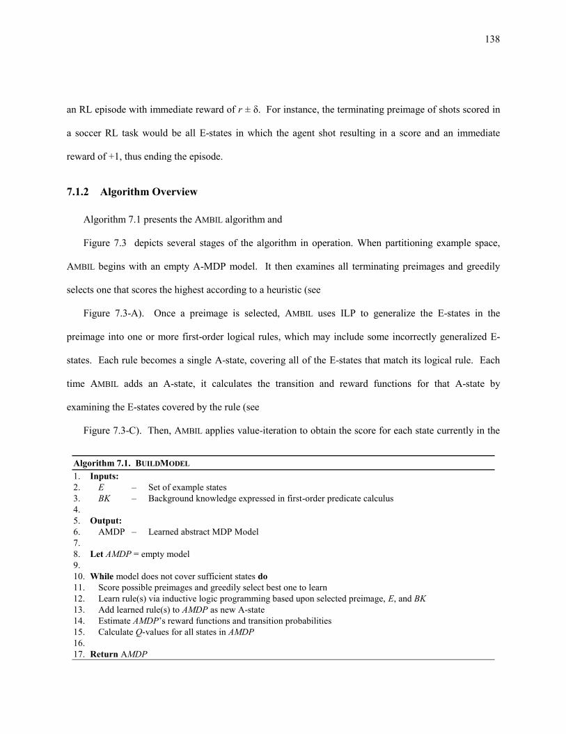
138

an RL episode with immediate reward of r ± δ. For instance, the terminating preimage of shots scored in

a soccer RL task would be all E-states in which the agent shot resulting in a score and an immediate

reward of +1, thus ending the episode.

7.1.2 Algorithm Overview

Algorithm 7.1 presents the AMBIL algorithm and

Figure 7.3 depicts several stages of the algorithm in operation. When partitioning example space,

AMBIL begins with an empty A-MDP model. It then examines all terminating preimages and greedily

selects one that scores the highest according to a heuristic (see

Figure 7.3-A). Once a preimage is selected, AMBIL uses ILP to generalize the E-states in the

preimage into one or more first-order logical rules, which may include some incorrectly generalized E-

states. Each rule becomes a single A-state, covering all of the E-states that match its logical rule. Each

time AMBIL adds an A-state, it calculates the transition and reward functions for that A-state by

examining the E-states covered by the rule (see

Figure 7.3-C). Then, AMBIL applies value-iteration to obtain the score for each state currently in the

Algorithm 7.1. BUILDMODEL

1. Inputs:

2. E – Set of example states

3. BK – Background knowledge expressed in first-order predicate calculus

4.

5. Output:

6. AMDP – Learned abstract MDP Model

7.

8. Let AMDP = empty model

9.

10. While model does not cover sufficient states do

11. Score possible preimages and greedily select best one to learn

12. Learn rule(s) via inductive logic programming based upon selected preimage, E, and BK

13. Add learned rule(s) to AMDP as new A-state

14. Estimate AMDP’s reward functions and transition probabilities

15. Calculate Q-values for all states in AMDP

16.

17. Return AMDP

139

A-MDP. This process repeats, greedily selecting from all previously unlearned terminating preimages

and A-state preimages (see

Figure 7.3-D, E, F) until the A-MDP covers at least a user-specified fraction of the example states.

7.1.3 Preimage Selection

When constructing an A-MDP, AMBIL greedily selects preimages to define the A-MDP. These

preimages consist of E-states not currently covered by some A-state and lead to a previously learned A-

state or a terminating preimage.

E(r) = 0

E(r) = 1

P = 0.66

P = 0.33

E(r) = 0

E(r) = 1

P = 0.66

P = 0.33

r = 1

r = 1

r = 0

r = 0

r = 0

r = 0

r = 0

r = 0

H1=0

H2=1

H3=0

E(r) = 0

E(r) = 1

P = 0.66

P = 0.33

S1=0.66

E(r) = 0

E(r) = 1

P = 0.66

P = 0.33

S1=0.66

H1=0

H2=0.66

H3=0.66S1=0.66

P = 1

S2=0.66 S1=0.66

P = 1

S2=0.66

P = 0.5

P = 0.5

S3=0.33

A B C

D E F“Uncovered”

Figure 7.3. Sample A-MDP being built in a 2D continuous state space. (A) E-states (open dots), reached

by two actions (solid and dotted arcs). Actionss reaching filled dots terminated the episode. (B) Initial

terminating preimages considered for learning, with their heuristic scores Hi shown, based upon the

rewards in the example data. (C) An A-MDP state learned based upon preimage H2. Note the A-state S1

could cover more example states than intended. Action arcs show the aggregate reward and transition

functions for S1. All calculations use γ=1. (D) Next stage of preimage selection and scoring. (E) A-MDP

extended by generalizing preimage H3 into A-state S2. (F) Final A-MDP after all preimages have been

generalized. Note some transitions, such as the top one from S3, may not lead to a learned A-state and are

placed in a special “uncovered” A-state, with a score of zero.

140

A simple heuristic scores each eligible preimage by an optimistic Q-value using Bellman-backups

(Bellman, 1957), according to equation (7.1). The optimistic Q-value represents the expected Q-value of

the preimage’s constituent E-states. Thus, the value is the expected reward of a transition from an E- state

in the preimage to the destination A-state via action a. This value is optimistic since it assumes AMBIL

can learn the preimage exactly and the example data is an i.i.d. sample of all possible E-states in the

preimage. In RL domains, this will not be true, since the distribution of E-states visited depends upon the

policy of the learner. In addition, the rule(s) learned to represent the preimage will often cover parts of

example space that were not part of the preimage. Even though the optimistic Q-value is inaccurate, it

serves as a good heuristic to guide preimage selection.

Preimage(S, )

( , ) (S)

(Preimage(S, ))Preimage(S, )

opt

s a

r s a Q

Q aa

(7.1)

Given the current A-MDP, only a subset of the possible preimages are eligible for learning. AMBIL

ignores preimages learned previously. Each preimage must contain a minimum number of E-states,

guaranteeing that enough data will be available for the rule-learning stage. Preimages must also obtain a

minimum optimistic Q-value score. This eliminates preimages unlikely to result in an increase in

performance.

AMBIL exploits the relational nature of the domain during preimage selection. It considers preimages

with multiple actions whenever the user indicates that two or more actions share similar behavior (via a

AMBIL specific configuration file). In these cases, the preimage will be parameterized appropriately for

each action. For instance, two shooting actions, such as shoot(left) and shoot(right) used in Section 8.5’s

experiments, might be considered together as shoot(GoalPart), where GoalPart is a logic variable

parameterizing the portion of the goal the shot was aimed at. This grouping allows AMBIL to exploit the

relational nature of some actions. Even when these groupings exist, AMBIL also considers the single-

action preimages since parameterized concepts may be more difficult to learn or specialized versions of

141

actions might be needed, depending on the task (e.g., shoot(left) and shoot(right) may make sense to

combine since they are symmetrical actions; however, shoot(center) may benefit from a specific shoot-

center rule.)

When AMBIL first creates an A-MDP, the MDP will contain no states to use as a basis for preimages.

Thus, AMBIL currently uses terminating preimages to initiate the MDP-building process (recall, a

terminating preimage is a set of E-states s = { s’ | s’ terminates the episode via action a }.) In the domains

I have focused on, clearly defined terminating preimages exist (e.g., shots resulting in a scored goal).

AMBIL could also use a domain’s reward-structure information, if available, to determine the initial

preimages. In non-sparse or infinite-horizon domains with no user-provided objective, AMBIL could

cluster the sampled rewards to determine initial concepts.

7.1.4 Learning Concepts via ILP

For each preimage selected, AMBIL uses inductive logic programming (ILP) to generate first-order

rules that describe the set of E-states that the preimage covers. Given an E-state, the learned rules classify

whether or not it is in the preimage, i.e. whether it leads to the relevant A-state via the indicated action or

not. Although AMBIL could use simpler propositional methods to learn the preimage classification, ILP

allows the relational aspect of the domain to be exploited: similar actions can be parameterized and

learned as a single concept, similar domain objects can be generalized, and extensive background

knowledge can be utilized to aid in describing the preimages. AMBIL uses the ILP system Aleph

(Srinivasan, 2001).

AMBIL selects the positive and negative ILP examples based upon the preimage being learned. For a

preimage(s, a), the E-states that transition to A-state S via action a, AMBIL collects, as positive examples,

all E-states where the action a was taken and the following E-state is covered by state S. The negative

examples are the E-states where action a was taken and the following state is not covered by S. E-states

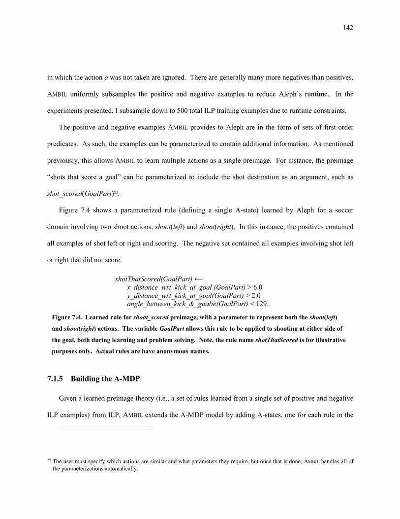
142

in which the action a was not taken are ignored. There are generally many more negatives than positives.

AMBIL uniformly subsamples the positive and negative examples to reduce Aleph’s runtime. In the

experiments presented, I subsample down to 500 total ILP training examples due to runtime constraints.

The positive and negative examples AMBIL provides to Aleph are in the form of sets of first-order

predicates. As such, the examples can be parameterized to contain additional information. As mentioned

previously, this allows AMBIL to learn multiple actions as a single preimage. For instance, the preimage

“shots that score a goal” can be parameterized to include the shot destination as an argument, such as

shot_scored(GoalPart)25.

Figure 7.4 shows a parameterized rule (defining a single A-state) learned by Aleph for a soccer

domain involving two shoot actions, shoot(left) and shoot(right). In this instance, the positives contained

all examples of shot left or right and scoring. The negative set contained all examples involving shot left

or right that did not score.

7.1.5 Building the A-MDP

Given a learned preimage theory (i.e., a set of rules learned from a single set of positive and negative

ILP examples) from ILP, AMBIL extends the A-MDP model by adding A-states, one for each rule in the

25 The user must specify which actions are similar and what parameters they require, but once that is done, AMBIL handles all of

the parameterizations automatically.

Figure 7.4. Learned rule for shoot_scored preimage, with a parameter to represent both the shoot(left)

and shoot(right) actions. The variable GoalPart allows this rule to be applied to shooting at either side of

the goal, both during learning and problem solving. Note, the rule name shotThatScored is for illustrative

purposes only. Actual rules are have anonymous names.

shotThatScored(GoalPart) ⟵

x_distance_wrt_kick_at_goal (GoalPart) > 6.0

y_distance_wrt_kick_at_goal(GoalPart) > 2.0

angle_between_kick_&_goalie(GoalPart) < 129.

143

theory. While AMBIL treats the separate rules from a theory independently, an A-state could be

represented by the complete theory. However, since a separate rule may represent different aspects of the

learned preimage introducing multiple A-states per learned theory increases the specificity of the final

model.

While AMBIL treats the learned model as an A-MDP, the model might not actually be one. Often, the

created model violates the Markovian assumptions required by MDPs and might be better characterized

as a partially observable Markov decision process26 (Sondik, 1971). However, in my experiments, even

when the Markovian assumptions were clearly violated, treating the model as an MDP still yielded good

results and made the calculation of the value function much faster.

In a proper MDP, states are discrete and disjoint. However, many of the A-states overlap with either

other A-states within a single preimage’s theory or other A-states previously added to the MDP. In order

to enforce disjointness among A-MDP states, AMBIL orders the states by their creation order, essentially

creating an IF-ELSEIF-ELSE structure used to determine in which A-state an E-state belongs. When

AMBIL adds multiple rules from a single preimage’s theory, the created A-states are ordered according to

their m-estimate adjusted accuracy on the Aleph training set.

After adding A-states to the A-MDP, AMBIL calculates the MDP’s state-transition probabilities and

reward functions. AMBIL computes the transition probability from MDP A-state S to MDP A-state S’ via

action a by counting the number of E-states that are covered by S and lead to S’ via action a, normalizing

these counts by the number of times action a was taken in state S. Similarly, it calculates the expected

reward for action a from A-state S by averaging over the rewards seen in the training data. AMBIL

employs m-estimates to condition the transition probabilities. I use m = 5 in my experiments. In some

26 Partially observable Markov decisions processes (POMDP) allow states in which a attributes or values of the state are

unknown. This allows the Markovian assumptions to be partially circumvented by including “hidden” variables in the state

definition. The discussion of POMDPs is beyond the scope of this document.

144

cases, E-states will exist that are not covered by any A-state. AMBIL assigns these E-states to a special

default state called the uncovered A-state.

After it calculates the transition probabilities and rewards, AMBIL performs value-iteration (Sutton &

Barto, 1998) for all A-states in the A-MDP, except the special uncovered A-state. The uncovered state’s

Q-value is some domain-dependent “background” score (e.g., zero). This discourages actions that would

lead to the uncovered state. Although not necessary in our experiments, AMBIL could utilize refinements

of the standard value-iteration algorithm, such as prioritized sweeping (Moore & Atkeson, 1993), to

increase the efficiency of the Q-value calculates.

When adding A-states to the A-MDP, AMBIL must address several additional considerations. If two

or more A-states overlap, A-states added later may not have adequate data. If the amount of data

available to an A-state is below some minimum threshold (currently, five E-states), AMBIL discards that

particular A-state.

On occasion, when AMBIL adds a state, the policy action it recommends (the argmax Q over all

actions for this state) is not the same as the action of the original preimage. When the action does not

match the preimage, this is indicative of one of two things: either a state does not have adequate data or

Aleph improperly generalized the preimage. In these cases, AMBIL could discard the MDP state.

However, in our experiments, this occurs infrequently and discarding the states is unnecessary.

7.1.6 The RL Learning Cycle

The previous sections described the process AMBIL uses to build a single A-MDP (and the associated

policy). In the complete learning cycle for a given RL domain, AMBIL first gathers some initial data by

interacting with the domain. It then repeatedly generates A-MDPs with a corresponding policy and

interacts with the domain following the new policy to gather more data. In each iteration, AMBIL

attempts to generate a new, higher-scoring policy.

145

Since the AMBIL model-building process is computationally expensive, AMBIL may not want to

rebuild a full model whenever new data is available. However, incrementally updating the reward and

transition functions for the A-MDP between full builds is computationally feasible and does result in

some improvement of the policy. I use this approach in the empirical results section below.

To gather initial data AMBIL either explores the domain randomly or uses another RL learning

algorithm (e.g., standard model-free Q-learning as a bootstrap). In domains with very sparse rewards

under a random policy, the bootstrapping process is preferred since it is more likely to obtain informative

data. After an A-MDP exists, when interacting with the RL domain, given an E-state, AMBIL determines

the action to perform by matching the E-state against the A-states in the A-MDP model. The argmax of

the Q-values for all actions for a given state determines the policy for that state. Additionally, as done by

standard RL algorithms, AMBIL performs a small fraction of exploratory actions.

7.2 Experiments

I present empirical results in two domains: a synthetic RL domain and the Breakaway RL domain

(Maclin, Shavlik, Torrey, Walker, & Wild, 2005), a subtask of the RoboCup soccer domain. I compare

AMBIL with the standard SARSA(λ) (Sutton & Barto, 1998) algorithm and with a model-learning

approach based upon a Dyna-Q architecture (Sutton, 1991). I chose Dyna-Q as a control because it is an

established approach for creating models of an environment in order to speed up RL.

7.2.1 Methodology

The synthetic domain, shown in Figure 7.5, is a simple five-state, three-action, non-deterministic

MDP, with two numeric features (drawn from overlapping uniform distributions), and a sparse reward

structure, with the only reward occurring in one of two terminating states. I purposefully overlap the

feature values for each state to simulate uncertainty in determining the underlying MDP state. I provided

146

the learners no direct knowledge of the underlying MDP. They must interact with the domain to obtain

information.

My Breakaway state representation is that of Maclin et al. (2005). For the Q-learner, I discretize

these features into 32 overlapping intervals called tiles, each of which becomes a Boolean feature. Stone

and Sutton (2001) used this enhancement in RoboCup; tiling allows linear function approximators to

represent non-linear concepts.

For Breakaway, the AMBIL background knowledge consists of feature_less_than,

feature_greater_than, feature_in_range, and feature_not_in_range predicates. Additionally, the

background includes predicates that provide information relative to passes and kicks. For example,

x_distance_wrt_kick measures the distance from the kicker to an object along the direction of the kick.

The background knowledge was designed to allow Aleph to discretize the base features.

All three learning algorithms, AMBIL, SARSA(λ), and Dyna-Q, are implemented as batch learners

and, as much as possible, I used the same tuning parameters on the standard Q-learner, giving the benefit

of doubt to the experimental control. Parameters were tuned on the Q-learning base line and used for the

other learners. Each learner “batch learns” every 25 games. All use an exploration rate of 1% and a

discount factor of 0.97. For the Q-learner and Dyna-Q I used a λ setting with λ=1 for recent E-states

decaying to λ=0 after a fixed number of games (200 for Breakaway, 50 for the synthetic MDP).

Figure 7.5. Synthetic domain MDP. Arcs represent state-transitions for three separate actions. All

actions are deterministic. S4 and S5 are terminating state. All rewards are zero, except for the single

action leading from S3 to S5.

r=1

S1 S2 S3

S4

S5

147

Both AMBIL and Dyna-Q use the standard Q-learning algorithm until enough data is available to start

the respective algorithm. Fifty and 250 games are played prior to Dyna/AMBIL running for the synthetic

and Breakaway domains, respectively.

Dyna-Q creates models that predict the feature values in the next state and the reward function of the

domain directly from the data and then uses the models to train Q-functions. I modeled the reward

function using a C4.5 decision tree (Quinlan, 1993). Next state feature values are modeled independently

of each other using support vector regression. I attempted to make these models as accurate as possible,

although modeling high-dimensional, real-valued environments is known to be difficult. The next state

models created by Dyna-Q are used to create synthetic examples. These examples are then utilized in the

same manner as real examples. I created enough synthetic data to maintain a 4-1 ratio of actual examples

to synthetic examples.

For the Breakaway domain, I also attempted to implement an RRL algorithm (Džeroski, De Raedt, &

Blockeel, 1998), a combination of traditional Q-learning with a relational TILDE-RT (Blockeel & De

Raedt, 1998) function approximator. Unfortunately, I was unable to obtain results better than random

walks with this approach.

7.2.2 Results

Figure 7.6 shows the average reward per game for the synthetic domain. Figure 7.7 shows the

average reward per game for the 2-on-1 Breakaway domain. For both domains, I performed 10 runs of

each algorithm and averaged the results. The reward per game is averaged over the previous 50 games

for the synthetic domain and previous 250 games for the Breakaway domain.

148

7.2.3 Discussion

In both domains, AMBIL outperformed both the Q-learner and the Dyna-Q algorithms, both in terms

of early learning rate and asymptotic performance. Several factors contribute to AMBIL’s early

Figure 7.7. 2-on-1 Breakaway; average reward received per game, averaged over previous 250 games.

0

0.1

0.2

0.3

0.4

0.5

0.6

0.7

0 250 500 750 1000 1250 1500

Ave

rage

Sco

re

Games Played

AMBIL

Q-Learner

Dyna-Q

Figure 7.6. Synthetic Domain; average reward received per game, averaged over previous 50 games.

0

0.1

0.2

0.3

0.4

0.5

0.6

0.7

0.8

0 100 200 300 400

Ave

rage

Sco

re

Games Played

AMBIL

Q-Learner

Dyna-Q

149

performance gains over the Q-learner. The background knowledge I provide to AMBIL offers it an

advantage. I attempted to provide propositionalized versions of the background knowledge to the standard

Q-learner, but this resulted in worse performance, presumably due to overfitting allowed by the greatly

increased number of features.

Beyond the background knowledge, AMBIL’s models, by construction, focus on reaching high-reward

states immediately and generalizing accurately. In Q-learning, on the other hand, reward information

propagates slowly through the model by the means of SARSA(λ) backups and generalization performed

by function approximation can be inaccurate, especially early in the learning curve.

The Dyna-Q implementation performed poorly in both domains. This was due to the difficulty of

modeling the underlying domain directly. It is the difficulty of this type of modeling that motivated

AMBIL’s approach.

7.3 Related Work

Reinforcement learning using TD methods has been studied extensively. Sutton and Barto (1998)

provide an excellent summary of the basic techniques. Dietterich and Flann (1995) introduced the

concept of using chains of preimages in their explanation-based reinforcement learning. Their action

chaining approach shares some basic similarities with AMBIL. However, their approach requires an

accurate definition of the action consequences. Kersting et al. (2004) create abstract relational MDPs

with many similarities to our own models. However, their approach to learning abstract MDPs requires

the underlying MDP. I essentially provide a learning method capable of learning a similar abstract MDP

in complex domains without knowledge of the underlying MDP be provided.

Morales’ (2003) rQ-learning provides a state-abstraction approach to reinforcement learning,

although their approach does not use an MDP representation. Unlike AMBIL, which learns the abstract

states, Morales’ approach requires user-provided abstractions. However, rQ-learning supports STRIPs-

150

like operators with more richness then AMBIL’s actions and provides a learning algorithm for refining

these operators. Van Otterlo’s (2003) CARCASS system provides a relational MDP representation,

similar to AMBIL’s, and provides methods to score and use the resulting MDP based upon interaction with

the domain. Like rQ-learning, Van Otterlo’s methods assume user-provided abstractions.

As an alternative approach to building an MDP, Džeroski et al. (1998) proposed using a relational

decision tree, such as TILDE , during Q-learning. Like AMBIL, this allows for both the integration of

background knowledge and the exploitation of the relational aspects of actions and objects in the domain.

However, like Q-learning, their approach represents only the long-term expected reward and does not

model the immediate reward or transition information, while AMBIL does. Furthermore, they are still

performing function approximation, which can be difficult for RL. Lecoeuche (2001) and Driessens et al.

(2001), among others, further refined this approach.

Another recent approach to relational reinforcement learning, by Zettlemoyer et al. (2005), also

models the domain without building an abstract MDP. Instead, they learn probabilistic STRIPs-like rules.

A probabilistic planner uses these rules to solve the domain. Like AMBIL, they focus on the state

transitions resulting from observed actions, although the rule learning process and final model does not

resemble AMBIL’s.


Models of reinforcement-learning tasks can allow faster learning than model-free Q-learning

methods, as demonstrated in my empirical study, and provide information about the structure of the

domain. My algorithm, AMBIL, builds relational abstract MDPs via inductive logic programming

techniques, focusing on areas of high reward to guide search. The use of ILP techniques allows our

models to represent relational domains, with abstraction of both objects and actions, and allows the

incorporation of background knowledge.

151

Furthermore, this technique illustrates an important aspect of advice giving, namely that ILP

background knowledge can be automatically acquired. In essence, the AMBIL algorithm plays the role of

the non ILP expert, providing “advice” to the ILP system that is then used to learn additional concepts.

Although not explored here, the rules learned by AMBIL could be used as a transfer mechanism to help

learn related reinforcement-learning tasks. Again, this transferred knowledge could be considered as

advice, produced by AMBIL and used to aid in learning the new task.

152

8 Additional Explorations – Building Relational Macros

for Transfer in Reinforcement Learning

In this chapter, I further explore the automated creation of background knowledge for use in transfer

learning. Transfer learning approaches take advantage of relationships between similar tasks, using

knowledge learned in a source task to speed up learning in a related target task. Algorithms that allow

successful transfer represent progress towards making machine learning as effective as human learning.

One area in which transfer is often desirable is reinforcement learning (RL), since standard RL

algorithms can require long training times. The RL domain that I use in this work is the simulated soccer

project RoboCup (Kitano, 1997). Several algorithms for transfer in domains like RoboCup have been

proposed. In Torrey et. al. (2006), we introduce an approach that transfers skills using inductive logic

programming (ILP), where a skill is a type of action that the RL learner uses. In this chapter, I extend that

approach by transferring strategies, which are action plans that may require composing several skills. I

continue to use ILP to learn strategies, and I represent them with a structure that I call a relational macro.

A relational macro is a finite-state machine (FSM) that uses first-order logic for decision-making. An

FSM is a model consisting of a set of nodes and transitions. To use a macro, an RL agent takes transitions

to move between nodes representing internal states, and it chooses actions to take in each node. Its

hold ← truepass(Teammate) ←

isOpen(Teammate)

isClose(Opponent)

¬ isClose(Opponent)

Figure 8.1. A possible strategy for the RoboCup game KeepAway, in which the RL agent in possession of

the soccer ball must execute a series of hold or pass actions to prevent its opponents from getting the ball.

The rules inside nodes show how to choose actions. The labels on arcs show the conditions for taking

transitions. Each node has an implied self-transition that applies by default if no exiting arc applies.

153

choices are determined by first-order logical clauses. Figure 8.1 shows a simple example of a relational

macro.

We use inductive logic programming (ILP) to learn macros because domains like RoboCup are

inherently relational. To our knowledge, fully relational RL approaches have not yet been successfully

applied in domains as complex as RoboCup. However, as shown previously (Torrey, Shavlik, Walker, &

Maclin, 2006), relational information can be successfully transferred between RoboCup tasks. Therefore,

we continue to use ILP in this approach, describing source-task behavior and relational macros in first-

order logic.

Relational-macro transfer begins by examining existing source-task episodes and analyzing them to

learn a successful strategy in the form of a macro. Section 8.3 describes our algorithm for this learning

stage. There are several possible ways to use the macro to improve learning in the target task; we use it to

demonstrate the successful strategy, as described in Section 8.5. After a short demonstration period that

gives the target-task learner a head start, we continue learning the task with standard RL. We call this

approach Relational Macro Transfer via Demonstration (RMT-D).

The work presented in this chapter was performed in collaboration with several others and previously

published (Torrey, Shavlik, Walker, & Maclin, 2007). I mostly participated in the ILP learning aspects of

this work, while the much of the design was done by L. Torrey.

8.1 Related Work in Transfer Learning

The goal in transfer learning is to speed up learning in a target task by transferring knowledge from a

related source task. One straightforward way to do this in reinforcement learning is to begin performing

the target task using the learned source-task models. Taylor et al. (2005) use this type of transfer method,

which we refer to as model reuse.

154

Another approach that has been proposed is to follow source-task policies during the exploration

steps of normal RL in the target task, instead of doing random exploration. This approach is referred to as

policy reuse and is performed by Fernandez and Veloso (2006). Our previous work includes a method

called skill transfer (Torrey, Shavlik, Walker, & Maclin, 2006). In skill transfer, we learn rules with ILP

that indicate when the agent chooses to take a single source-task action. There are multiple ways that

these skills could be used in the target task; we use an advice-taking approach in this previous work. Our

advice places soft constraints on the target-task solution that can be followed or ignored according to how

successful they are. Taylor and Stone (2007) also learn a set of rules for taking actions, and they propose

different advice-taking mechanisms: for instance, they give a Q-value bonus to the advised action.

There are also approaches for transferring multi-step action sequences, such as those of Perkins and

Precup (1999) and Soni and Singh (2006). Known as options, these sequences have their own internal Q-

functions that are followed until they reach a termination state. The target-task learner treats options as

alternative actions. Croonenborghs et al. (2007) learn relational options for use in relational reinforcement

learning (RRL). Options are often used in hierarchical RL (Dietterich, 2000) as well as in transfer

learning.

We propose to perform transfer by learning relational macros and using them to demonstrate

successful behavior in the target task. Our approach is related to several of the methods described above.

It could be viewed as a type of model reuse or policy reuse that creates an abstract version of the source-

task model instead of reusing it directly. Like skill transfer, it uses ILP, but it involves multi-step

strategies instead of single actions. It shares the idea of transferring sub-policies with option transfer, but

an option traditionally represents a single policy while a macro contains a separate sub-policy at each

node.

155

8.2 Executing a Relational Macro

We have defined a relational macro as a finite-state machine (Gill, 1962). An FSM models the

behavior of a system in the form of a directed graph. The nodes of the graph represent states of the

system, and in our case they represent internal states of the agent in which different policies apply.

The policy of a node can be to take a single action, such as move(ahead) or shoot(goalLeft), or to

choose from a class of actions, such as pass(Teammate). In the latter case, a node uses first-order logical

clauses to decide which grounded action to choose. An FSM begins in a start node and has conditions for

transitioning between nodes. In a relational macro, these conditions are also sets of first-order logical

clauses.

Figure 8.1 show a sample macro from the KeepAway reinforcement task. When executing this

macro, a KeepAway agent begins in the initial node on the left. The only action it can choose in this node

is hold. It remains there, taking the default self-transition, until the condition isClose(Opponent) becomes

true for some opponent player. Then it transitions to the second node, where it evaluates the

pass(Teammate) rule to choose an action. If the rule is true for just one teammate player, it passes to that

teammate; if several teammates qualify, it randomly chooses between them; if no teammate qualifies, it

abandons the macro and reverts to using the Q-function to choose actions. The receiving teammate then

becomes the learning agent, and it remains in the pass node if an opponent is close or transitions back to

the hold node otherwise.

Figure 8.1 is a simplification in one respect: each transition and node in a macro has an entire set of

rules, rather than just one rule. This allows us to represent disjunctive conditions. When more than one

grounded action or transition is possible (when multiple rules match), the agent obeys the rule that has the

highest score. The score of a rule is the estimated probability that following it will lead to a successful

game. We estimate these probability scores from source-task data.

156

8.3 Learning a Relational Macro

We learn a macro by analyzing source-task data. We assume that this data is available because we

have previously learned the source task and stored the games27 generated during the learning process. The

method by which the source task was learned is not particularly important, since the data we use only

consists of states, actions, and rewards. In reinforcement learning, as the policy become better defined

and more stable, later games tend to have less variance and there is less variety in the states encountered

and action taken. Thus, when selecting the training from the source-task, it is important that the data

include game from early in the learning curve as well as later to guarantee that the training data is diverse.

In our system, we include all 3000 games from the source-task learning curve.

Given this data, we use inductive logic programming (ILP) to characterize successful behavior in the

source task. Specifically, we use a locally modified version of Aleph (Srinivasan, 2001). Given a set of

positive and negative training examples, the Aleph algorithm selects a positive “seed” example, builds the

most specific clause that entails the example within the provided language restrictions, and searches for a

more general clause that maximizes a provided scoring function.

The precision of a rule is the fraction of examples it calls positive that are truly positive, and the

recall is the fraction of truly positive examples that it correctly calls positive. We use the F1 scoring

function

(8.1)

because as it balances precision and recall, both of which are important when learning macros. We use

both the heuristic and randomized search algorithms provided by Aleph.

27 Each game consists of a sequence of states and actions. Throughout this research we look at a soccer task and thus the

sequence of actions a game. It might be more accurate to call the sequence a trajectory or episode.

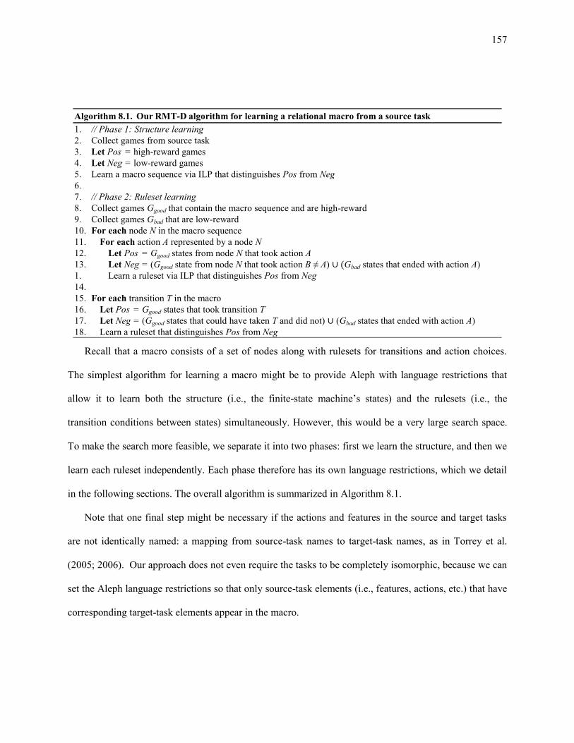
157

Recall that a macro consists of a set of nodes along with rulesets for transitions and action choices.

The simplest algorithm for learning a macro might be to provide Aleph with language restrictions that

allow it to learn both the structure (i.e., the finite-state machine’s states) and the rulesets (i.e., the

transition conditions between states) simultaneously. However, this would be a very large search space.

To make the search more feasible, we separate it into two phases: first we learn the structure, and then we

learn each ruleset independently. Each phase therefore has its own language restrictions, which we detail

in the following sections. The overall algorithm is summarized in Algorithm 8.1.

Note that one final step might be necessary if the actions and features in the source and target tasks

are not identically named: a mapping from source-task names to target-task names, as in Torrey et al.

(2005; 2006). Our approach does not even require the tasks to be completely isomorphic, because we can

set the Aleph language restrictions so that only source-task elements (i.e., features, actions, etc.) that have

corresponding target-task elements appear in the macro.

Algorithm 8.1. Our RMT-D algorithm for learning a relational macro from a source task

1. // Phase 1: Structure learning

2. Collect games from source task

3. Let Pos = high-reward games

4. Let Neg = low-reward games

5. Learn a macro sequence via ILP that distinguishes Pos from Neg

6.

7. // Phase 2: Ruleset learning

8. Collect games Ggood that contain the macro sequence and are high-reward

9. Collect games Gbad that are low-reward

10. For each node N in the macro sequence

11. For each action A represented by a node N

12. Let Pos = Ggood states from node N that took action A

13. Let Neg = (Ggood state from node N that took action B ≠ A) (Gbad states that ended with action A)

1. Learn a ruleset via ILP that distinguishes Pos from Neg

14.

15. For each transition T in the macro

16. Let Pos = Ggood states that took transition T

17. Let Neg = (Ggood states that could have taken T and did not) (Gbad states that ended with action A)

18. Learn a ruleset that distinguishes Pos from Neg

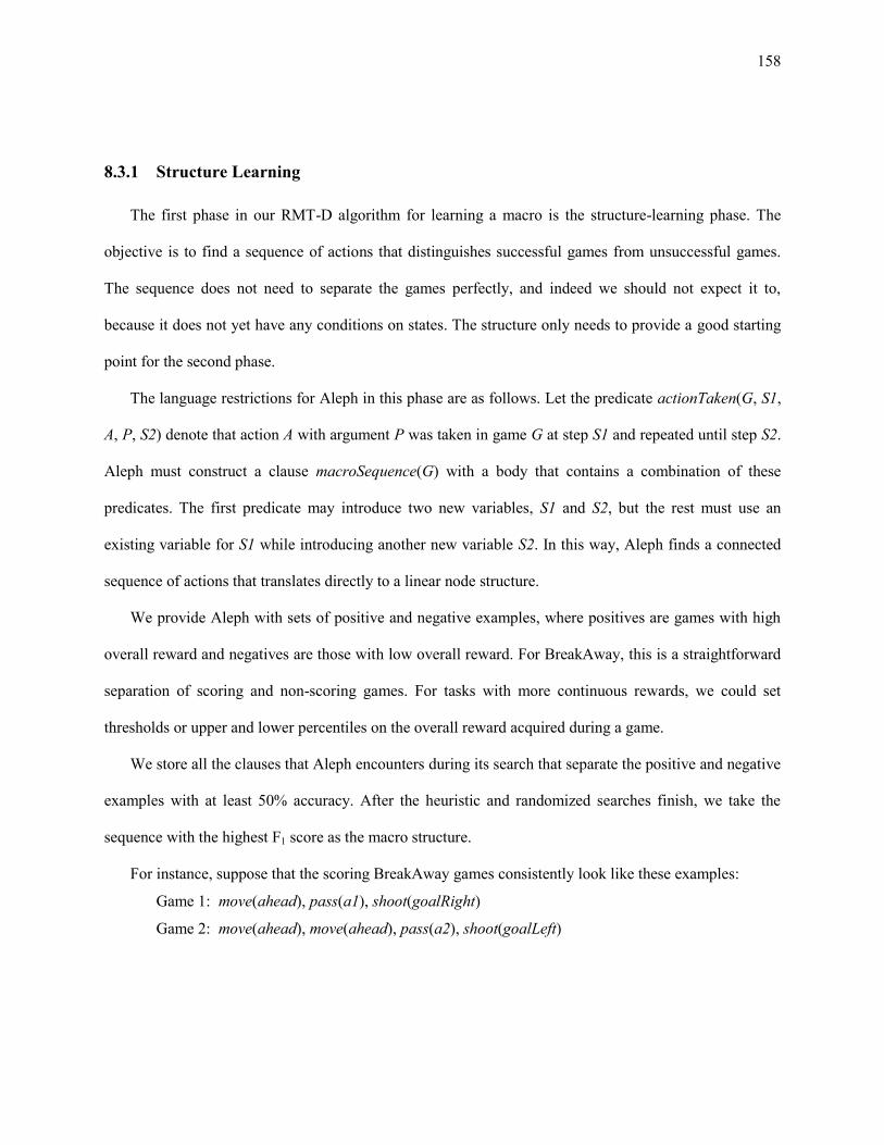
158

8.3.1 Structure Learning

The first phase in our RMT-D algorithm for learning a macro is the structure-learning phase. The

objective is to find a sequence of actions that distinguishes successful games from unsuccessful games.

The sequence does not need to separate the games perfectly, and indeed we should not expect it to,

because it does not yet have any conditions on states. The structure only needs to provide a good starting

point for the second phase.

The language restrictions for Aleph in this phase are as follows. Let the predicate actionTaken(G, S1,

A, P, S2) denote that action A with argument P was taken in game G at step S1 and repeated until step S2.

Aleph must construct a clause macroSequence(G) with a body that contains a combination of these

predicates. The first predicate may introduce two new variables, S1 and S2, but the rest must use an

existing variable for S1 while introducing another new variable S2. In this way, Aleph finds a connected

sequence of actions that translates directly to a linear node structure.

We provide Aleph with sets of positive and negative examples, where positives are games with high

overall reward and negatives are those with low overall reward. For BreakAway, this is a straightforward

separation of scoring and non-scoring games. For tasks with more continuous rewards, we could set

thresholds or upper and lower percentiles on the overall reward acquired during a game.

We store all the clauses that Aleph encounters during its search that separate the positive and negative

examples with at least 50% accuracy. After the heuristic and randomized searches finish, we take the

sequence with the highest F1 score as the macro structure.

For instance, suppose that the scoring BreakAway games consistently look like these examples:

Game 1: move(ahead), pass(a1), shoot(goalRight)

Game 2: move(ahead), move(ahead), pass(a2), shoot(goalLeft)

159

Assuming that the non-scoring games have different patterns than the examples above do, Aleph

might learn the following clause to characterize a scoring game:

macroSequence(Game) ←

actionTaken(Game, StateA, move, ahead, StateB),

actionTaken(Game, StateB, pass, Teammate, StateC),

actionTaken(Game, StateC, shoot, GoalPart, gameEnd).

The macro structure corresponding to this sequence is shown in Figure 8.2. The policy in the first

node will be to take a single action, move(ahead). In the second node the policy will be to consider

multiple pass actions, and in the third node the policy will be to consider multiple shoot actions. The

conditions for choosing an action, and for taking transitions between nodes, are learned in the next phase.

8.3.2 Ruleset Learning

The second phase in our RMT-D algorithm for learning a macro is the ruleset-learning phase. The

objective is to describe when transitions and actions should be taken based on the RL state features. We

learn a ruleset for each transition and each action independently, so that we perform several smaller, in-

depth searches rather than one large search. Because of this, variables in these rules are local to a node

rather than global to the entire macro.

The language restrictions for Aleph in this phase are as follows. There is one predicate for each state

feature of the RL task (shown in Table 8.1). To describe the conditions on state S under which a transition

should be taken, Aleph must construct a clause transition(S) with a body that contains a combination of

move(ahead) pass(Teammate) shoot(GoalPart)

Figure 8.2. The structure that corresponds to the example macro clause in Section 8.3.1.

160

these predicates. To describe the conditions under which an action should be taken, Aleph must construct

a clause action(S, Action, ActionArg).

Aleph may learn some action rules in which the action argument is grounded, such as action(S, move,

ahead), as well as rules in which the action argument remains a variable, such as action(S, pass,

Teammate). In the case of the move action in BreakAway the action argument in a rule is always

grounded, since the original state features do not include useful references to move directions. We could

have defined additional predicates that did, but we chose to use only the original features. Note that it is

still possible to have a state move(Direction) for taking multiple move actions, but the rules for choosing a

grounded move action will use only grounded arguments.

We provide Aleph with sets of positive and negative examples, consisting of states in source-task

games that took the transition or action. Consider the macro structure in Figure 8.2; we will describe the

action datasets for the pass node and the transition datasets for the transition from the move node to the

pass node. Let Ggood represent the set of high-reward source-task games that contain the macro sequence

and let Gbad represent the set of low-reward source-task games.

Table 8.1. BreakAway task features. Arguments with capitol letters are logical variables. A complete list

of task features is generated by replacing variables with all appropriate constants. The ClosestDefender

refers to the defender closest to the attacker currently holding the ball.

BreakAway features

distBetween(a0, Player)

distBetween(Attacker, ClosestDefender)

angleDefinedBy(Attacker, k0, ClosestDefender)

xPosition(Object)

yPosition(Object)

distBetween(Attacker, goalCenter)

distBetween(a0, GoalPart)

angleDefinedBy(GoalPart, a0, goalie)

angleDefinedBy(topRight, goalCenter, a0)

distBetween(Attacker, goalie)

angleDefinedBy(Attacker, a0, goalie)

timeLeft

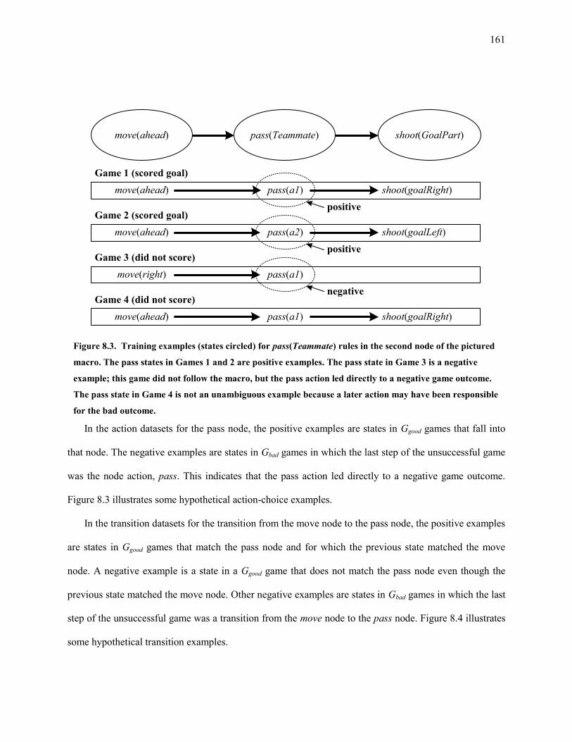
161

In the action datasets for the pass node, the positive examples are states in Ggood games that fall into

that node. The negative examples are states in Gbad games in which the last step of the unsuccessful game

was the node action, pass. This indicates that the pass action led directly to a negative game outcome.

Figure 8.3 illustrates some hypothetical action-choice examples.

In the transition datasets for the transition from the move node to the pass node, the positive examples

are states in Ggood games that match the pass node and for which the previous state matched the move

node. A negative example is a state in a Ggood game that does not match the pass node even though the

previous state matched the move node. Other negative examples are states in Gbad games in which the last

step of the unsuccessful game was a transition from the move node to the pass node. Figure 8.4 illustrates

some hypothetical transition examples.


move(ahead) pass(a1) shoot(goalRight)

Game 1 (scored goal)

move(ahead) pass(a2) shoot(goalLeft)


move(right) pass(a1)

Game 3 (did not score)



positive

positive

negative

Figure 8.3. Training examples (states circled) for pass(Teammate) rules in the second node of the pictured

macro. The pass states in Games 1 and 2 are positive examples. The pass state in Game 3 is a negative

example; this game did not follow the macro, but the pass action led directly to a negative game outcome.

The pass state in Game 4 is not an unambiguous example because a later action may have been responsible

for the bad outcome.

162

As in the first phase, we store all the clauses that Aleph encounters during the search that classify the

training data with at least 50% accuracy. However, instead of selecting a single best clause as we did in

the previous phase, we collect from these a ruleset for each transition and each action. We wish to have

one strategy (i.e. one finite-state machine), but there may be multiple reasons for making internal choices.

Our procedure for greedily selecting which clauses are included in a ruleset is summarized in

Algorithm 8.2. We sort the rules by decreasing precision and walk through the list, adding rules to the

final ruleset if they increase the set's recall and do not decrease its F1 score.

We assign each rule a score that may be used to decide which rule to obey if multiple rules match

while executing the macro. The score is an estimate of the probability that following the rule will lead to a

successful game. We determine this estimate by collecting training-set games that followed the rule and

calculating the fraction of these that ended successfully.




move(ahead) shoot(goalLeft)


move(ahead) pass(a1)


positive

negative

shoot(goalRight)

Figure 8.4. Training examples (states circled) for the transition from move to pass in the pictured macro.

The pass state in Game 1 is a positive example. The shoot state in Game 2 is a negative example; the game

began by following the macro but did not take the transition from move to pass. The pass state in Game 3

is not an unambiguous example because a later step may have been responsible for the bad outcome.

163

8.4 Transferring a Relational Macro

Our target-task learner begins by simply executing the macro strategy for a set of episodes, instead of

exploring randomly as an untrained RL agent would traditionally do. In this demonstration period, we

generate examples of Q-values: each time the macro chooses an action because a high-scoring rule

matched, we use the rule score to estimate the Q-value of the action. Recall the rule score is the estimated

probability that following the rule leads to a successful game. Since BreakAway has Q-values ranging

from zero to one, we simply set the estimate equal to the rule score (if this were not the case, we could

multiply the probability by an appropriate scaling factor to fit a larger Q-value range). We also use rule

scores to produce Q-value estimates for other actions for which rules fired. Finally, we infer that actions

for which no rules fired had very low Q-values, which in the BreakAway domain we estimate as zero.

Note that the examples with low estimated Q-values are necessary to ensure that the initial Q-function

is not overly optimistic in unexplored areas. Driessens and Džeroski (2004) also encountered this problem

in their work on guidance in RRL; they addressed it by interleaving imitation with exploration.

For each step of the demonstration we therefore have a Q-value estimate for each action, and via

support vector regression we use these to learn an initial Q-function for the target task. The demonstration

period lasts for 100 games in our system, and as usual after each batch of 25 games we relearn the Q-

Algorithm 8.2. The RMT-D procedure for selecting the final ruleset for one transition or action.

1. Let R = all rules encountered with > 50% accuracy

2. Let S = R sorted by decreasing precision on the training set

3. Let T = ∅

4.

5. For each rule r ∊ S do

6. Let W = T r }

7. If recall(W) > recall(T ) and score(W) score(T ) then

8. Let T = W

9.

10. Return FinalRuleset = T

164

function. After 100 games, we continue learning the target task with standard RL. This generates new Q-

value examples in the standard way, and we combine these with the old macro-generated examples as we

continue relearning the Q- function after each batch. As the new examples accumulate, we gradually drop

the old examples by randomly removing them at the rate that new ones are being added.

Since standard RL has to act mostly randomly in the early steps of a task, a good macro strategy can

provide a large immediate advantage. The performance level of the demonstrated strategy is unlikely to

be as high as the target-task agent can achieve with further training, unless the tasks are similar enough to

make transfer a trivial problem, but the hope is that the learner can smoothly improve its performance

from the level of the demonstration up to its asymptote. If there is limited time and the target task cannot

be trained to its asymptote, then the immediate advantage that macros can provide may be even more

valuable in comparison to methods like skill transfer.

8.5 Experimental

8.5.1 Methodology

We present results from transfer experiments with RMT-D in the RoboCup domain. To test our

approach, we learn a macro from data acquired while training 2-on-1 BreakAway and transfer it to both 3-

on-2 and 4-on-3 BreakAway. We learn the source task with standard RL for 3000 games, and then we

train the target tasks for 3000 games to show both the initial advantage of the macros and the behavior

as training continues.

8.5.2 Results

Figure 8.5 and Figure 8.6 show our results in 3-on-2 and 4-on-3 BreakAway respectively. We

compare our approach against Q-learning as well as two related transfer methods: model reuse (Taylor,

Stone, & and Liu, 2005) and skill transfer (Torrey, Shavlik, Walker, & Maclin, 2006). Each curve in the

165

figure is an average of 25 runs and has points smoothed over the previous 500 games to smooth over

the high variance in the RoboCup domain. For the transfer algorithms, there are five target-task runs

generated from each of five source-task runs, to allow for variance in both stages of learning.

Our agents in 2-on-1 BreakAway reach a performance asymptote of scoring in approximately 70% of

the episodes. The macros learned from the 2-on-1 source runs, when executed in 2-on-1 BreakAway,

score in approximately 50% of the episodes. (A random policy scores in less than 1% of the episodes.)

The macros therefore appear to capture the majority of the successful behavior of the source task, though

they do not describe it completely. Capturing source-task behavior more completely, while avoiding

overfitting, is one topic for future work.

Figure 8.5. Probability of scoring a goal in 3-on-2 BreakAway, with Q-learning and with three transfer

approaches that use 2-on-1 BreakAway as the source task.

0

0.1

0.2

0.3

0.4

0.5

0.6

0 500 1000 1500 2000 2500 3000

Pro

bab

ility

of

Go

al

Training Games

Standard RL

Model Reuse

Skill Transfer

Relational Macro

166

8.5.3 Discussion

The macros that RMT-D learned from the five source runs all had similar structures. The most

common version is shown in Figure 8.7. In one of the runs the initial pass node was not included, and

the ordering of shoot(goalRight) and shoot(goalLeft) varied, as would be expected in the symmetrical

BreakAway task. The presence of two shoot nodes may seem counterintuitive, but it appears that the RL

agent uses the first shot as a feint to lure the goalie in one direction, counting on a teammate to intercept

the shot before it reaches the goal. When it does, the learning agent switches to the teammate in

possession of the ball and performs the second shot, which is actually intended to score. This tendency of

RL agents to use actions in unintended (or creative) ways is an indication of the difficulties that can arise

when learning relational concepts from RL data.

Figure 8.6. Probability of scoring a goal in 4-on-3 BreakAway, with Q-learning and with three transfer

approaches that use 2-on-1 BreakAway as the source task.

0

0.1

0.2

0.3

0.4

0.5

0.6

0 500 1000 1500 2000 2500 3000

Pro

bab

ility

of

Go

al

Training Games

Standard RL

Model Reuse

Skill Transfer

Relational Macro

167

All of the transfer algorithms speed up learning in comparison to Q-learning, but the benefits they

provide are different. Model reuse and relational macros both provide an advantage in the early

performance of the target-task learner. RMT-D produces a larger advantage in these scenarios than model

reuse does, and it scales better as the distance between the source and target grows. Skill transfer provides

no initial benefit, but then develops a steady advantage over Q-learning. During the middle section of the

learning curve it performs slightly better than RMT-D before they all converge at the asymptote.

In pointwise t-test comparisons at the 99% confidence level, the RMT-D curve is significantly

above the model-reuse curve for the first 1100 episodes in Figure 8.5 and 1425 episodes in Figure 8.6.

The RMT-D curve is significantly above the skill-transfer curve for the first 575 episodes in Figure 8.5

and 875 episodes in Figure 8.6. The skill-transfer curve is significantly above the RMT-D curve at just

one point in Figure 8.5 (at 1825 episodes) and never in Figure 8.6, and the model-reuse curve is never

significantly above the RMT-D curve in either figure.

We also tried an algorithm that combines skill transfer via advice with RMT- D. The combination is

straightforward: we begin by demonstrating the macro as in RMT-D, and we incorporate advice when

learning the Q-function as in skill transfer. This produces a learning curve (not shown) that is not

significantly different from the RMT-D curve. The substantial early effects of transferring a macro via

demonstration apparently overwhelm the effects of skill-transfer advice.

move(Teammate) move(Direction) shoot(goalRight) shoot(goalLeft)

Figure 8.7. One of the five macro structures learned from 2-on-1 BreakAway runs. There are between 10

and 20 rules associated with each transition and action, so those are not shown.

168


I described an approach for transferring relational macros from a source task that gives the target-task

learner a significant head start. Our relational-macro approach makes extensive use of ILP during

learning, demonstrating ILP in applications, i.e., transfer and reinforcement learning, not typically

associated with ILP. As with the work presented in Chapter 7, the use of relational macros for transfer

can be considered a form of advice giving in which the ILP-learned relational macro is the advice. This

again highlights the power of using relational advice along with ILP.

Although not investigated here, one interesting future direction would be to further refine the

relational macro after transferring it to the target task. The refinement might take the form of updating

the parameters or structure of a macro based on early experience in the target task or might entail learning

a completely new relational macro. In this second scenario, instead of using the transferred macro to

demonstrate a good policy, the transferred macro could be provided to the target-task learner as advice.

Other possible extensions to this work include alternative macro designs that may capture the source-

task behavior more completely. While a single linear action sequence appears to explain the majority of

our agents' success in the source task, other configurations might perform better. Using probabilistic

approaches, such as statistical relational learning, to estimate probabilities and to make decisions from

rulesets would also be an interesting extension.

Finally, our RMT-D algorithm is most effective when the user is confident that the source-task

strategy is a reasonable approximation of a good target-task strategy. However, relational macros might

be applicable in more distant transfer scenarios, such as when only part of a source-task strategy is useful

in a target task. This might require alternative approaches to applying the relational macros in the target

task, which might again involve a form of refinement of the original relational macro, as mentioned

above.

169

9 Conclusions

Relational supervised learning approaches, such as inductive logic programming (ILP), can be

powerful learning tools. However, these approaches are generally difficult to use, requiring in-depth

expertise. This thesis presents my original research aimed at reducing the level of expertise necessary to

employ these algorithms. The complexity of relational approaches stems primarily from three different

tasks:

1. Specify background knowledge.

2. Define the hypothesis space.

3. Select and tune required parameters.

In Chapter 4, I examined an approach that addresses the creation of background knowledge and

hypothesis-space specification by experts whose expertise lies outside of ILP. I based the approach on an

advice-taking paradigm, allowing the user to provide advice as to why specific examples in an ILP

problem are either positive or negative. Since the advice pertains to specific examples, the user does not

need to understand logic programming nor ILP. My approach translates the provided advice into

generalized background knowledge usable by the ILP system. Additionally, I generate the required

hypothesis space specification automatically, alleviating the need for the user to understand that aspect of

ILP.

In Chapter 5, I further extended my advice-taking approach by examining the use a human-computer

interface (HCI). The HCI further reduces the difficulty of providing advice. I proposed an iterative

method of learning with advice taking, in which the user can repeatedly specify advice, followed

immediately by learning and evaluation of the learned model, after which the user can provide further

advice (or refine previously provided advice). This approach can take advantage of probabilistic

relational learning algorithms to assist the user in determining which examples where highly misclassified

170

and need to be corrected the most. Additionally, I introduced the intelligence, surveillance, and

reconnaissance (ISR), an important application that demonstrates the benefits of this iterative HCI advice-

taking approach.

In Chapter 6, I presented an automated method, the ONION, for tuning the ILP parameters. The

approach uses an iterative-deepening style search, iteratively expanding the search space, trying different

parameter combinations, and stopping when the ILP learns an acceptable theory. I showed that the

ONION algorithm performs well without any user interaction. This approach again relieves the burden of

the user when it comes to configuring and running ILP.

Future Work

Although my contributions solve some of the difficulties of using ILP, there are still many aspects of

ILP learning that could be improved through further research. First, while the automated generation of

background knowledge through advice-giving is a powerful mechanism, the approach has limitations.

One of the major limitations is that the advice can often be ambiguous. In the current approach, I resolve

this introducing multiple interpretation of the advice as background knowledge and allowing the ILP

search process to determine the interpretation that fits the data. However, the number of interpretations

grows exponentially as the complexity of the advice grows, limiting the effectiveness of this approach. A

better solution might be to allow the user to provide information to determine which interpretations are

likely to be the correct ones. Additional research should examine what that additional information might

be and how the user might specify it, while keeping in the spirit of not forcing the user to understand the

underlying ILP algorithm.

Another open area of study is how to expose the underlying power of ILP to the user, again without

forcing the user to understand the underlying algorithm. My current approach necessarily hides much of

the underlying ILP configuration, but in doing so, some of the power of ILP is lost. This is a particularly

difficult problem, but I believe an HCI approach might again be useful, perhaps by presenting the user

171

with feedback during the search and allowing the user to adjust how the search progress, essentially

changing the underlying configuration according to the input from the user.

Finally, and perhaps most importantly, it would be advantageous to apply my advice-taking paradigm

to a more diverse set of relational algorithms. Statistical relational learning (SRL) algorithms (Getoor &

Taskar, 2007) that combine logical and probabilistic techniques present many of the same difficulties for

the non-expert user that ILP does. In some cases, my techniques apply directly to SRL algorithms with

little change, as I demonstrated with bRDNs (Natarajan, Khot, Kersting, Gutmann, & Shavlik, 2010). In

other cases, additional work is needed to determine how to apply this work to these algorithms.

Overall Conclusion

My contributions, considered together and validated on multiple diverse testsets, provide solutions for

many of the issues encountered when using ILP. The advice-taking paradigm is easily understood by non

ILP experts, especially when the advice pertains to specific examples. The addition of an HCI alleviates

the need for the non ILP expert to understand the ILP configuration file format or syntax while providing

direct feedback to the user, further assisting in learning. The ONION alleviates the last major difficulty by

providing automated parameter tuning.

172

References

Alphonse, E., & Matwin, S. (2002). Feature subset selection and inductive logic programming. In the

Proceedings of the Nineteenth International Conference on Machine Learning.

Bellman, R. (1957). Dynamic Programming. Princeton University Press.

Blockeel, H., & De Raedt, L. (1998). Top-down induction of first-order logical decision trees. Artificial

Intelligence, 101:1-2.

Cerny, V. (1985). A thermodynamical approach to the travelling salesman problem: An efficient

simulation algorithm. Journal of Optimization Theory and Applications, 45:41-51.

Chen, J., & Weld, D. (2008). Recovering from errors during programming by demonstration. In the

Proceedings of the International Conference on Intelligent User Interfaces.

Church, A. (1936). An unsolvable problem of elementary number theory. American Journal of

Mathematics, 58, 345–363.

Cristianini, N., & Shawe-Taylor, J. (2000). Support Vector Machines and Other Kernel-Based Learning

Methods. Cambridge University Press.

Croonenborghs, T., Driessens, K., & Bruynooghe, M. (2007). Learning relational skills for inductive

transfer in relational reinforcement learning. In the Proceedings of the Seventeenth International

Conference on Inductive Logic Programming.

Croonenborghs, T., Ramon, J., Blockeel, H., & Bruynooghe, M. (2006). Model-assisted approaches for

relational reinforcement learning: Some challenges for the SRL community. In the Proceedings

of the ICML Workshop on Open Problems in Statistical Relational Learning.

Cypher, A. (1993). Watch What I Do: Programming by Demonstration. The MIT Press.

De Raedt, L. (1992). Interactive Theory Revision: An Inductive Logic Programming Approach. Academic

Press.

Devijver, P., & Kittler, J. (1982). Pattern Recognition: A Statistical Approach. Prentice-Hall.

Dietterich, T. (2000). Hierarchical reinforcement learning with the MAXQ value function decomposition.

Journal of Artificial Intelligence Research, 13:227-303.

173

Dietterich, T., & Flann, N. (1995). Explanation-based learning and reinforcement learning: A unified

view. In the Proceedings of the Twelfth International Conference on Machine Learning.

Dietterich, T., Ashenfelter, A., & Bulatov, Y. (2004). Training conditional random fields via gradient tree

boosting. In the Proceedings of the Twenty-first International Conference of Machine Learning.

Driessens, K., & Džeroski, S. (2004). Integrating guidance into relational reinforcement learning.

Machine Learning, 57:271-304.

Driessens, K., Ramon, J., & Blockeel, H. (2001). Speeding up relational reinforcement learning through

the use of an incremental first order decision tree algorithm. In the Proceedings of the Twelfth

European Conference on Machine Learning.

Džeroski, S., De Raedt, L., & Blockeel, H. (1998). Relational reinforcement learning. In the Proceedings

of the Eighth International Conference on Inductive Logic Programming.

Fails, J., & Olsen, D. (2003). Interactive machine learning. In the Proceedings of the International

Conference on Intelligent User Interfaces 2003.

Fernandez, F., & Veloso, M. (2006). Policy reuse for transfer learning across tasks with different state and

action space. ICML Workshop on Structural Knowledge Transfer for Machine Learning.

Finn, P., Muggleton, S., Page, D., & Srinivasan, A. (1998). Discovery of pharmacophores using the

inductive logic programming system Progol. Special issue of Machine Learning on Applications

and the Knowledge Discovery Process, 30(1-2), 241-270.

Fung, G., Mangasarian, O., & Shavlik, J. (2002). Knowledge-based support vector machine classifiers. In

the Proceedings of Neural Information Processing Systems.

Getoor, L., & Taskar, B. (2007). Introduction to Statistical Relational Learning. The MIT Press.

Gill, A. (1962). Introduction to the Theory of Finite-state Machines. McGraw-Hill.

Gödel, K. (1929). On the Completeness of theLogical Calculus. Ph.D Dissertation, University Of Vienna.

Gutmann, B., & Kersting, K. (2006). Tildecrf: Conditional random fields for logical sequences. In the

Proceedings of the Seventeenth European Conference of Machine Learning.

Heckerman, D., Chickering, D., Meek, C., Rounthwaite, R., & Kadie., C. (2001). Dependency networks

for inference, collaborative, and data visualization. Journal of Machine Learning Research, 1:49-

75.

174

Horn, A. (1951). On sentences which are true of direct unions of algebras. Journal of Symbolic Logic,

16:14–21.

Huang, T., & Mitchell, T. (2006). Text clustering with extended user feedback. In the Proceedings of the

Special Interest Group on Information Retrieval.

ISO/IEC-13211. (1995). Information technology — Programming languages — Prolog. International

Organization for Standardization. Geneva.

Kate, R., Wong, Y., Ge, R., & Mooney, R. (2004). Learning transformation rules for semantic parsing.

Computational linguistics and intelligent text processing: Proceedings of the Eighth International

Conference.

Kersting, K., Van Otterlo, M., & De Raedt, L. (2004). Bellman goes relational. In the Proceedings of the

twenty-first International Conference on Machine Learning.

Kitano, H. (1997). RoboCup: The robot world cup initiative. In the Proceedings of the First International

Conference on Autonomous Agent.

Kohavi, R., John, G., & Prieditis, A. (1995). Automatic parameter selection by minimizing estimated

error. In the Proceedings of the Twelfth International Conference on Machine Learning.

Koller, D., & Friedman, N. (2009). Probabilistic Graphical Models, Principles and Techniques. The MIT

Press.

Korf, R. (1985). Depth-first iterative-deepening: An optimal admissible tree search. Artificial Intelligence,

27:97-109.

Kowalski, R. (1973). Predicate logic as a programming language. Memo 70. Department of Artificial

Intelligence, Edinburgh University.

Lavrac, N., Gamberger, D., & Jovanosk, V. (1999). A study of relevance for learning in deductive

databases. Journal of Logic Programming, 40:215-249.

Lecoeuche, R. (2001). Learning optimal dialog management rules by using reinforcement learning and

inductive logic programming. In the Proceedings of the Second meeting of the North American

Chapter of the Association of Computational Linquistic.

Lieberman, H. (Ed.). (2001). Your Wish is My Command: Programming by Example. Morgan Kaufmann.

175

Maclin, R., Shavlik, J., Torrey, L., Walker, T., & Wild, E. (2005). Giving advice about preferred actions

to reinforcement learners via knowledge-based kernel regression. In the Proceedings of the

Twentieth Conference on Artificial Intelligence.

Mangasarian, O., Shavlik, J., & Wild, E. (2004). Knowledge-based kernel approximation. Journal of

Machine Learning Research, 5:1127-1141.

McDaniel, R., & Myers, B. (1999). Getting more out of programming-by-demonstration. In the

Proceedings on Human Factors in Computing Systems.

Mendenhall, W., Wackerly, D., & Scheaffer, R. (1989). Nonparametric statistics. In Mathematical

Statistics with Applications (4th ed.) (pp. 674–679). PWS-Kent.

Mitchell, T. (1997). Machine Learning. McGraw Hill.

Moore, A., & Atkeson, C. (1993). Prioritized sweeping: Reinforcement learning with less data and less

time. Machine Learning, 13:103-130.

Morales, F. (2003). Scaling up reinforcement learning with a relational representation. In the Proceedings

of the Workshop on Adaptablility in Multi-Agent Systems at AORC’03.

Mozina, M., Zabkar, J., & Bratko, I. (2007). Argument based machine learning. Artificial Intelligence,

171, 10-15.

Muggleton, S. (1987). DUCE, an oracle based approach to constructive induction. In Proceedings of the

Tenth International Joint Conference on Artificial Intelligence.

Muggleton, S. (1995). Inverse entailment and Progol. New Generation Computing, 13, 245-286.

Muggleton, S., & Buntine, W. (1988). Machine invention of first-order predicates by inverting resolution.

In the Proceedings of the Fifth International Conference on Machine Learning.

Muggleton, S., & Feng, C. (1992). Inductive logic programming. In S. Muggleton (Ed.), Efficient

Induction in Logic Programs (pp. 281-298). Academic Press.

Natarajan, S., Khot, T., Kersting, K., Gutmann, B., & Shavlik, J. (2010). Boosting relational dependency

networks. In the Proceedings of the Twenty-first International Conference on Inductive Logic

Programming.

Neville, J., & Jensen, D. (2007). Relational dependency networks. Journal of Machine Learning

Research, 8:653-692.

176

Oblinger, D. (2006). Bootstrap learning - external materials. Retrieved from http://www.sainc.com/bl-

extmat.

Pasula, H., Zettlemoyer, L., & Kaelbling, L. (2004). Learning probabilistic relational planning rules. In

the Proceedings of the Nineteenth Conference on Artificial Intelligence.

Pazzani, M., & Kibler, D. (1992). The utility of knowledge in inductive learning . Machine Learning, 9,

57-94.

Perkins, T., & Precup, D. (1999). Using options for knowledge transfer in reinforcement learning.

Technical Report UM-CS-1999-034. University of Massachusetts Amherst, MA.

Quinlan, J. (1990). Learning logical definitions from relations. Machine Learning, 5:239-266.

Quinlan, J. (1993). C4.5: Programs for Machine Learning. Morgan Kauffman.

Quinlan, J., & Cameron-Jones, R. (1995). Oversearching and layered search in empirical learning. In the

Proceedings of the Fourteenth International Joint Conference on Artificial Intelligence.

Richards, B., & Mooney, R. (1995). Automated refinement of first-order Horn-clause domain theories.

Machine Learning, 19: 95–131.

Richardson, M., & Domingos, P. (2006). Markovlogic networks. Machine Learning, 62:107-136.

Rummery, G., & Niranjan, M. (1994). On-line Q-learning using Connectionist Systems. Technical Report

CUED/F-INFENG/TR 166, Engineering Department, Cambridge University.

Russell, S., & Norvig, P. (2010). Artificial Intelligence: A Modern Approach (3nd ed.). Prentice Hall.

Sammut, C. (1981). Learning Concepts by Performing Experiments. Ph.D. Dissertation, Department of

Computer Science, University of New South Wales.

Settles, B. (2008). Curious Machines: Active Learning with Structured Instances. Ph.D. Dissertation,

Department of Computer Science, University of Wisconsin–Madison.

Shapiro, E. (1983). Algorithmic Program Debugging. The MIT Press.

Siekmann, J. (1990). An Introduction to Unification Theory. In R. Banerji (Ed.), Formal Techniques in

Artificial Intelligence - A Sourcebook. Elsevier Science Publishers.

Snyman, J. (2005). Practical Mathematical Optimization: An Introduction to Basic Optimization Theory

and Classical and New Gradient-Based Algorithms. Springer Publishing.

177

Sondik, E. (1971). The Optimal Control of Partially Observable Markov Processes. Ph.D. Dissertation,

Stanford Electronics Labs, Stanford University.

Soni, V., & Singh, S. (2006). Using homomorphisms to transfer options across continuous reinforcement

learning domains. In the Proceedings of the Twenty-first National Conference on Artificial

Intelligence.

Srinivasan, A. (2001). The Aleph Manual. Retrieved from

www.comlab.ox.ac.uk/activities/machinelearning/Aleph/aleph.

Srinivasan, A., King, R., Muggleton, S., & Sternberg, M. (1997). Carcinogenesis predictions using ILP.

Lecture Notes in Computer Science, 1297/1997, 273-287.

Srinivasan, A., Muggleton, S., & King, R. (1995). Comparing the use of background knowledge by

inductive logic programming systems. In the Proceedings of the Fifth ILP Workshop.

Stone, P., & Sutton, R. (2001). Scaling reinforcement learning toward RoboCup soccer. In the

Proceedings of the Eighteenth International Conference on Machine Learning.

Stumpf, S., Rajaram, V., Li, L., & Wong, W. (2009). Interacting meaningfully with machine learning

systems: Three experiments. International Journal of Human-Computer Studies, 67:639-662.

Sutton, R. (1988). Learning to predict by the methods of temporal differences. Machine Learning, 3, 9-

44.

Sutton, R. (1991). Dyna, an integrated architecture for learning, planning, and reacting. SIGART Bulletin,

2:160–163.

Sutton, R., & Barto, A. (1998). Reinforcement Learning: An Introduction. The MIT Press.

Taylor, M., & Stone., P. (2007). Cross-domain transfer for reinforcement learning. In the Proceedings of

the Twenty-fourth International Conference on Machine Learning.

Taylor, M., Stone, P., & and Liu, Y. (2005). Value functions for RL-based behavior transfer: A

comparative study. In the Proceedings of the twentieth National Conference on Artificial

Intelligence.

Torrey, L., Shavlik, J., Walker, T., & Maclin, R. (2006). Relational skill transfer via advice taking. In the

ICML'06 Workshop on Structural Knowledge Transfer for Machine Learning.

178

Torrey, L., Shavlik, J., Walker, T., & Maclin, R. (2006). Skill acquisition via transfer learning and advice

taking. In the Proceedings of the Seventeenth European Conference on Machine Learning.

Torrey, L., Shavlik, J., Walker, T., & Maclin, R. (2007). Relational macros for transfer in reinforcement

learning. In the Proceedings of the Seventeenth Conference on Inductive Logic Programming.

Torrey, L., Walker, T., Shavlik, J., & Maclin, R. (2005). Knowledge transfer via advice taking. In the

Proceedings of the Third International Conference on Knowledge Capture.

Van Otterlo, M. (2003). Efficient reinforcement learning using relational aggregation. In the Proceedings

of the Sixth European Workshop on Reinforcement Learning.

Vander Zanden, B., & Myers, B. (1995). Demonstrational and constraint-based techniques for pictorially

specifying application objects and behaviors. Transactions on Computer Human Interaction,

2:308-356.

Walker, T., Kunapuli, G., Larsen, N., Page, D., & Shavlik, J. (2011). Integrating knowledge capture and

supervised learning through a human-computer interface. In the Proceedings of Sixth

International Conference on Knowledge Capture.

Walker, T., O'Reilly, C., Kunapuli, G., Natarajan, S., Maclin, R., Shavlik, J., et al. (2010). Automating the

ILP setup task: Converting user advice about specific examples into general background

knowledge. In the Proceedings of the twentieth International Conference on Inductive Logic

Programming.

Wargus. (2002). Retrieved from http://wargus.sourceforge.net.

Watkins, C., & Dayan, P. (1992). Technical note: Q-learning. Machine Learning, 8:279-292.

Whitley, D., Dominic, S., Das, R., & Anderson, C. (1993). Genetic reinforcement learning for

neurocontrol problems. Machine Learning, 13:259-284.

Zettlemoyer, L., Pasula, H., & Kaelbling, L. (2005). Learning planning rules in noisy stochastic worlds.

In the Proceedings of the Twentieth Conference on Artificial Intelligence.

179

Nomenclature

Term Domain† Definition

accessor FOL Informally, a literal in a logical rule that introduces a variable representing the

property of an entity. For instance, color(ACar, Color) would access the color

property for the ACar entity.

action RL A Markov decision process element that represents one of the possible choices an

agent can select at each time step.

agent RL An entity that selects actions to perform, typically according to a learned policy.

background

knowledge

ILP The set of logical statements that are believed to be true in a ILP problem. Used to

determine if a given learned rule or theory entails an example.

Bellman equation RL An equation recursively defining the expected reward value of an RL state or state-

action pair.

Bellman-backups RL A sequence of recursive applications of the Bellman equation.

body ILP The set of negated literals in a definite clause corresponding to the antecedent of the

definite clause when in implication form.

boosted

relational

dependency

networks

(bRDN)

A specific classification supervised learning algorithm that uses first-order logic

rules and graphical models to provided probability based classification of examples

(Natarajan, Khot, Kersting, Gutmann, & Shavlik, 2010).

bootstrap

learning

A learning approach in which simple concepts are learned first, followed by more

difficult concepts that use (i.e., bootstrap from) the simpler concepts.

class One of two or more categories that a classification algorithm attempts to distinguish

between.

classification A supervised learning method where the example labels consist of two or more

classes and the goal is to learn a model that distinguishes between the classes.

clause ILP A disjunction of positive and negative literals. Informally, shorthand for a Horn

clause or a definite clause, depending on context.

clause learner ILP In an ILP algorithm, the inner-most loop that learns individual rules in the form of

definite clauses.

covered ILP Given a rule (or theory), an ILP examples is covered if the rule (or theory) and

background knowledge entails the example.

decision

boundary

The separating boundary between two classes in classification supervised learning.

definite clause ILP A Horn clause with exactly one positive literal.

determination ILP A configuration parameter specifying a predicate symbol to include in the ILP

search space, i.e., a literal that may appear in the body of a learned ILP rule.

error of omission A mistake in which knowledge is omitted.

180


fact ILP Informally, a definite clause consisting of a single positive literal. Typically used

to distinguish between definite clauses with and without a body in background

knowledge (i.e., a fact versus a rule.)

feature

description

The information detailing a single supervised learning example.

feature space The space of all possible feature descriptions for a given supervised learning task.

feature vector See fixed-length feature vector.

fixed-length

feature vector

A feature description of an example that consists of n feature values, where n is

fixed for all examples in a given learning task.

flip-flopping Informally, the processes of swapping the positive and negative examples sets

during ILP in order to learn a theory representing the negation of the target concept.

function

approximator

RL A regression function, typically used to estimate a Q-value given an input state and

action.

goal ILP A definite clause consisting of only negated literals. In SLD resolution, a query to

be resolved.

grid search A parameter-tuning approach where the cross-product of all possible parameter

combinations is exhaustively evaluated to find the best parameter settings.

Horn clause ILP A clause containing a set of disjunctive literals with at most one positive literal and

any number of negated literals.

kernel A positive definite function k(x,y) representing an inner-product between x and y.

knowledge-based

support vector

machine (KB-

SVM)

An extension to support vector machines that incorporates additional knowledge

when learning a model. The knowledge takes the form of inequalities specifying

the class for regions of the search space.

label In classification, the class of an example. In regression, the real value associated

with an example.

literal FOL Either the negation or non-negation of an atomic formula.

logic program FOL A list of logical statement that, along with an associated logical resolution

semantics (e.g., SLD resolution), which allows the truth value of a goal statement to

be evaluated.

Markov decision

process

A model formally describing a reinforcement-learning environment, consisting of a

5-tuple {S, A, P, R, } with a set S of states, a set A of actions, a probability

distribution P, a reward function R, and a discount factor ∈ ( .

maximum-

margin

A supervised learning technique that attempts to find the decision boundary that

separates the example classes while maximizing the minimum distance between the

boundary and examples.

max-margin See maximum-margin.

misclassification An incorrectly classified example.

model-based RL Reinforcement learning techniques that attempt to learn a model of the underlying

MDP.

181


model-free RL Reinforcement learning techniques that do not attempt to learn a model of the

underlying MDP, typically learning a value-function or Q-function directly.

modes ILP Constraints applied to the arguments of candidate literals in the ILP search space,

controlling both the type of an argument and its possible value.

parameter A configuration value for an algorithm that controls certain aspects of the

algorithm. Typically either specified by the user or tuned through some automated

method.

policy RL A function π : S A mapping states to action. Used to determine the action taken

by an RL agent for any given state.

Q-function RL A function Q : S × A that maps a given state and action to the expected

discounted reward for taking the action from the state.

regression A form of supervised learning in which the examples labels are real values and the

learned function maps examples to real values.

relevance

strength

ILP An indicator attached to literals in the ILP search space to indicate how likely they

are to occur in the learned rules.

reward RL The real-valued signal provided to an RL learning agent according to the reward

function R : S × A f the MD

supervised

learning

A form of machine learning where the input is a training set of examples and their

associated label, possibly along with additional information, and the output is a

model that predicts a label for (possibly unseen) examples.

target ILP The predicate symbol of the examples in an ILP task.

target predicate ILP See target.

theory ILP A collection of definite clauses rules logically conjoined. Used to represent

disjunctive concepts.

theory learner ILP A loop in the ILP learning process that repeated calls a clause learner and

assembles the returned clauses into a single theory.

transfer learning RL A form of learning in which information is extract from a source task in order to

learn a target task.

uncovered ILP Given a rule (or theory), an ILP examples is uncovered if the rule (or theory) and

background knowledge does not entail the example.

WILL ILP The Wisconsin Inductive Logic Learner.

† FOL F r t-Order Logic. RL = Reinforcement Learning. ILP = Inductive Logic Programming.

Computer Sciences Department -...

Documents

Transcript of Computer Sciences Department -...