Computer Science Technical Report

A Hybrid Method for the Verification and

Synthesis of Parameterized Weakly

Stabilizing ProtocolsAmer Tahat and Ali Ebnenasir

Michigan Technological UniversityComputer Science Technical Report

CS-TR-14-02May 2014

Department of Computer ScienceHoughton, MI 49931-1295

www.cs.mtu.edu

A Hybrid Method for the Verification and Synthesis of

Parameterized Weakly Stabilizing Protocols

Amer Tahat and Ali Ebnenasir

May 2014

Abstract

We present a hybrid method for verification and synthesis of parameterized self-stabilizing protocolswhere algorithmic design and mechanical verification techniques/tools are used hand-in-hand. The coreidea behind the proposed method includes the automated synthesis of self-stabilizing protocols in a limitedscope (i.e., fixed number of processes) and the use of theorem proving methods for the generalization ofthe solutions produced by the synthesizer. Specifically, we use the Prototype Verification System (PVS)to mechanically verify an algorithm for the synthesis of weakly self-stabilizing protocols. Then, we reusethe proof of correctness of the synthesis algorithm to establish the correctness of the generalized versionsof synthesized protocols for an arbitrary number of processes. We demonstrate the proposed approachin the context of an agreement and a coloring protocol on the ring topology.

1

Contents

1 Introduction 3

2 Formal Specifications of Basic Concepts 42.1 Protocols . . . . . . . . . . . . . . . . . . . . . . . . . . . . . . . . . . . . . . . . . . . . . . . 42.2 Distribution and Atomicity Models . . . . . . . . . . . . . . . . . . . . . . . . . . . . . . . . . 42.3 Computation . . . . . . . . . . . . . . . . . . . . . . . . . . . . . . . . . . . . . . . . . . . . . 52.4 Closure and Convergence . . . . . . . . . . . . . . . . . . . . . . . . . . . . . . . . . . . . . . 6

3 Problem Statement 6

4 Specification of Add Weak 7

5 Verification of Add Weak 75.1 Verifying the Equality of Projections on Invariant . . . . . . . . . . . . . . . . . . . . . . . . . 75.2 Verifying Weak Convergence . . . . . . . . . . . . . . . . . . . . . . . . . . . . . . . . . . . . . 8

6 Compound Grind Proof Technique 86.1 COMP GRIND Proof Technique . . . . . . . . . . . . . . . . . . . . . . . . . . . . . . . . . . 86.2 Recursive Nature of COMP GRIND . . . . . . . . . . . . . . . . . . . . . . . . . . . . . . . . 96.3 Complexity of COMP GRIND . . . . . . . . . . . . . . . . . . . . . . . . . . . . . . . . . . . 96.4 GRIND vs COMP GRIND . . . . . . . . . . . . . . . . . . . . . . . . . . . . . . . . . . . . . 10

7 Reusability and Generalizability 107.1 PVS Specification of Coloring . . . . . . . . . . . . . . . . . . . . . . . . . . . . . . . . . . . . 107.2 Mechanical Verification of Parameterized Coloring . . . . . . . . . . . . . . . . . . . . . . . . 12

8 Verifying the Convergence of Binary Agreement (AG) 138.1 PVS Specification of AG(n) . . . . . . . . . . . . . . . . . . . . . . . . . . . . . . . . . . . . . 13

8.1.1 Specifying the Processes . . . . . . . . . . . . . . . . . . . . . . . . . . . . . . . . . . . 148.1.2 Specifying the Parameterized Protocol AG(n) . . . . . . . . . . . . . . . . . . . . . . . 14

8.2 Weak Stabilization of Binary Agreement Protocol AG(n) . . . . . . . . . . . . . . . . . . . . . 14

9 Discussion and Related Work 15

10 Conclusion and Future Work 15

2

1 Introduction

Self-stabilization is an important property of dependable distributed systems as it guarantees convergence inthe presence of transient faults. That is, from any state/configuration, a Self-Stabilizing (SS) system recoversto a set of legitimate states (a.k.a. invariant) in a finite number of steps. Moreover, from its invariant, theexecutions of an SS system satisfy its specifications and remain in the invariant; i.e., closure. Nonetheless,design and verification of convergence are difficult tasks [10, 19] in part due to the requirements of (i) recoveryfrom arbitrary states; (ii) recovery under distribution constraints, where processes can read/write only thestate of their neighboring processes (a.k.a. their locality), and (iii) the non-interference of convergence withclosure. Methods for algorithmic design of convergence [2, 3, 16, 13] can generate only the protocols that arecorrect up to a limited number of processes and small domains for variables. Thus, it is desirable to devisemethods that enable automated design of parameterized SS systems, where a parameterized system includesseveral sets of symmetric processes that have a similar code up to variable re-naming.

Numerous approaches exist for mechanical verification of self-stabilizing systems most of which focus onsynthesis and verification of specific protocols. For example, Qadeer and Shankar [32] present a mechanicalproof of Dijkstra’s token ring protocol [10] in the Prototype Verification System (PVS) [34]. Kulkarni et al.[29] use PVS to mechanically prove the correctness of Dijkstra’s token ring protocol in a component-basedfashion. Prasetya [31] mechanically proves the correctness of a self-stabilizing routing protocol in the HOLtheorem prover [18]. Tsuchiya et al. [35] use symbolic model checking to verify several protocols such asmutual exclusion and leader election. Kulkarni et al. [28, 7] mechanically prove (in PVS) the correctnessof algorithms for automated addition of fault tolerance; nonetheless, such algorithms are not tuned for thedesign of convergence. Most existing automated techniques [5, 27, 14, 16] for the design of fault toleranceenable the synthesis of non-parametric fault-tolerant systems. For example, Kulkarni and Arora [27] presenta family of algorithms for automated design of fault tolerance in non-parametric systems, but they do notexplicitly address self-stabilization. Abujarad and Kulkarni [3] present a method for algorithmic design ofself-stabilization in locally-correctable protocols, where the local recovery of all processes ensures the globalrecovery of the entire distributed system. Farahat and Ebnenasir [13, 16] present algorithms for the design ofself-stabilization in non-locally correctable systems. Jacobs and Bloem [22] show that, in general, synthesisof parameterized systems from temporal logic specifications is undecidable. They also present a semi-decisionprocedure for the synthesis of a specific class of parameterized systems in the absence of faults.

The contributions of this paper are two-fold: a hybrid method (Figure 1) for the synthesis of parameter-ized self-stabilizing systems and a reusable PVS theory for mechanical verification of self-stabilization. Theproposed method includes a synthesis step and a theorem proving step. Our previous work [13, 16] enablesthe synthesis step where we take a non-stabilizing protocol and generate a self-stabilizing version thereofthat is correct by construction up to a certain number of processes. This paper investigates the second stepwhere we use the theorem prover PVS to prove (or disprove) the correctness of the synthesized protocolfor an arbitrary number of processes; i.e., generalize the synthesized protocol. The synthesis algorithms in[13, 16] incorporate weak and strong convergence in existing network protocols; i.e., adding convergence.Weak (respectively, Strong) convergence requires that from every state there exists an execution that (re-spectively, every execution) reaches an invariant state in finite number of steps. To enable the second step,we first mechanically prove the correctness of the Add Weak algorithm from [16] that adds weak convergence.As a result, any protocol generated by Add Weak will be correct by construction. Moreover, the mechanicalverification of Add Weak provides a reusable theory in PVS that enables us to verify the generalizabilityof small instances of different protocols generated by an implementation of Add Weak. If the mechanicalverification succeeds, then it follows that the synthesized protocol is in fact correct for an arbitrary numberof processes. Otherwise, we use the feedback of PVS to determine why the synthesized protocol cannot begeneralized and re-generate a protocol that addresses the concerns reported by PVS. We continue this cycleof synthesize and generalize until we have a parameterized protocol. Notice that the theory developed inmechanical proof of Add Weak can also be reused for the mechanical verification of self-stabilizing protocolsdesigned by means other than our synthesis algorithms. We demonstrate this reusability in the context of acoloring protocol (Section 7) and a binary agreement protocol (Appendix B).Organization. Section 2 introduces basic concepts and presents their formal specifications in PVS. Then,

3

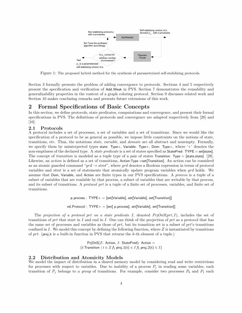
Figure 1: The proposed hybrid method for the synthesis of parameterized self-stabilizing protocols.

Section 3 formally presents the problem of adding convergence to protocols. Sections 4 and 5 respectivelypresent the specification and verification of Add Weak in PVS. Section 7 demonstrates the reusability andgeneralizability properties in the context of a graph coloring protocol. Section 9 discusses related work andSection 10 makes conclusing remarks and presents future extensions of this work.

2 Formal Specifications of Basic ConceptsIn this section, we define protocols, state predicates, computations and convergence, and present their formalspecifications in PVS. The definitions of protocols and convergence are adapted respectively from [28] and[10].

2.1 ProtocolsA protocol includes a set of processes, a set of variables and a set of transitions. Since we would like thespecification of a protocol to be as general as possible, we impose little constraints on the notions of state,transitions, etc. Thus, the notations state, variable, and domain are all abstract and nonempty. Formally,we specify them by uninterpreted types state: Type+, Variable: Type+, Dom: Type+, where ‘+’ denotes thenon-emptiness of the declared type. A state predicate is a set of states specified as StatePred: TYPE = set[state].The concept of transition is modeled as a tuple type of a pair of states Transition: Type = [state,state] [28].Likewise, an action is defined as a set of transitions, Action:Type =set[Transition]. An action can be considredas an atomic guarded command “grd→ stmt”, where grd denotes a Boolean expression in terms of protocolvariables and stmt is a set of statements that atomically update program variables when grd holds. Weassume that Dom, Variable, and Action are finite types in our PVS specifications. A process is a tuple of asubset of variables that are readable by that process, a subset of variables that are writable by that process,and its subset of transitions. A protocol prt is a tuple of a finite set of processes, variables, and finite set oftransitions.

p process : TYPE+ = [set[Variable], set[Variable], set[Transition]]

nd Protocol : TYPE+ = [set[ p process], set[Variable], set[Transition]]

The projection of a protocol prt on a state predicate I, denoted PrjOnS(prt, I), includes the set oftransitions of prt that start in I and end in I. One can think of the projection of prt as a protocol that hasthe same set of processes and variables as those of prt, but its transition set is a subset of prt’s transitionsconfined in I. We model this concept by defining the following function, where Z is instantiated by transitionsof prt. (proj k is a built-in function in PVS that returns the k-th element of a tuple.)

PrjOnS(Z: Action, I: StatePred): Action =

{t:Transition | t ∈ Z∧

proj 1(t) ∈ I∧

proj 2(t) ∈ I}

2.2 Distribution and Atomicity ModelsWe model the impact of distribution in a shared memory model by considering read and write restrictionsfor processes with respect to variables. Due to inability of a process Pj in reading some variables, eachtransition of Pj belongs to a group of transitions. For example, consider two processes P0 and P1 each

4

having a Boolean variable that is not readable for the other process. That is, P0 (respectively, P1) canread and write x0 (respectively, x1), but cannot read x1 (respectively, x0). Let 〈x0, x1〉 denote a state ofthis program. Now, if P0 writes x0 in a transition (〈0, 0〉, 〈1, 0〉), then P0 has to consider the possibilityof x1 being 1 when it updates x0 from 0 to 1. As such, executing an action in which the value of x0 ischanged from 0 to 1 is captured by the fact that a group of two transitions (〈0, 0〉, 〈1, 0〉) and (〈0, 1〉, 〈1, 1〉)is included in P0. In general, a transition is included in the set of transitions of a process iff (if and onlyif) its associated group of transitions is included. Formally, any two transitions (s0, s1) and (s′0, s

′1) in a

group of transitions formed due to the read restrictions of a process Pj meet the following constraints,where rj denotes the set of variables Pj can read: ∀v : v ∈ rj : (v(s0) = v(s′0)) ∧ (v(s1) = v(s′1)) and∀v : v /∈ rj : (v(s0) = v(s1)) ∧ (v(s′0) = v(s′1)), where v(s) denotes the value of a variable v in a state s. Toenable the reusability of our PVS specifications, we specify our distribution model as a set of axioms so onecan mechanically prove convergence under different distribution and atomicity models.

In the following formal specifications, v is of type Variable, p is of type p process, t and t′ are of type Tran-

sition, and non read and transition group are functions that respectively return the set of unreadable variablesof the process p and the set of transitions that meet ∀v : v ∈ rj : (v(s0) = v(s′0)) ∧ (v(s1) = v(s′1)) for atransition t = (s0, s1) and its groupmate t′ = (s′0, s

′1).

AXIOM subset?(proj 2(p),proj 1(p)) // Writeable variables are a subset of readable variables.

AXIOM member(t′,transition group(p, t, prt)) AND member(v,Non read(p, prt))

IMPLIES Val(v,proj 1(t)) = Val(v,proj 2(t)) AND Val(v,proj 1(t′)) = Val(v,proj 2(t′))

member(x,X) and subset?(X,Y) respectively represent the membership and subset predicates in a set-theoretic sense.

2.3 ComputationA computation of a protocol prt is a sequence A of states, where (A(i), A(i + 1)) represents a transition ofprt executed by some action of prt. In a more general term, a computation of any set of transitions Z, is asequence of states in which every state can be reached from its predecessor by a transition in Z. Thus, wedefine the following function to return the set of computations generated by the set of transitions Z.

COMPUTATION(Z: Action): set[sequence[state]]={ A: sequence[state] |∀(n : nat) : ((A(n), A(n + 1)) ∈ Z)}

A computation prefix of a protocol prt is a finite sequence of states where each state is reached from itspredecessor by a transition of prt. Kulkarni et al. [28] specify a prefix as an infinite sequence in which onlya finite number of states are used. By contrast, we specify a computation prefix as a finite sequence type.We believe that it is more natural and more accurate to model the concept of prefix by finite sequences. Ourexperience also shows that modeling computation prefixes as finite sequences simplifies formal specificationand verification of reachability and convergence while saving us several definitions that were required in[28] to capture the length of the prefix. In the specification of computation prefixes, we use the predicateCondi prefix?(A,Z) that holds when all transitions (A(i), A(i+1)) of a sequence A belong to a set of transitionsZ. The notation A‘length denotes the length of the sequence A and A‘seq(i) returns the i-th element of sequenceA.

Pos F S: TYPE = {c:finite sequence[state] | c‘length > 0}

Condi Prefix?(A:Pos F S,Z:Action):bool= FORALL(i: below[A‘length-1] ): member((A‘seq(i), A‘seq(i+1)), Z)

PREFIX(Z: Action): set[Pos F S]= {A:Pos F S | Condi Prefix?(A,Z) }

5

2.4 Closure and ConvergenceA state predicate I is closed in a protocol prt iff every transition of prt that starts in I also terminates in I[19, 4]. The closed predicate checks whether a set of transitions Z is actually closed in a state predicate I.

closed?(I: StatePred, Z: Action): bool = FORALL (t:Transition | (member(t,Z)) AND member(proj 1(t), I)) :

member(proj 2(t), I)

A protocol prt weakly converges to a non-empty state predicate I iff from every state s, there exists atleast one computation prefix that starts in s and reaches some state in I [19, 4]. A strongly convergingprotocol guarantees that every computation from s will reach some state in I. Notice that any stronglyconverging protocol is also weakly converging, but the reverse is not necessarily true. A protocol prt isweakly (respectively, strongly) self-stabilizing to a state predicate I iff (1) I is closed in prt, and (2) prtweakly (respectively, strongly) converges to I from any state.

3 Problem StatementThe problem of adding convergence (from [16]) is a transformation problem that takes as its input a protocolprt and a state predicate I that is closed in prt. The output of Problem 3.1 is a revised version of prt,denoted prtss, that converges to I from any state. Starting from a state in I, prtss generates the samecomputations as those of prt; i.e., prtss behaves similar to prt in I.

Problem 3.1 Add Convergence

• Input: (1) A protocol prt; (2) A state predicate I such that I is closed in prt; and (3) A property ofLs converging, where Ls ∈ {weakly, strongly}.

• Output: A protocol prtss such that : (1) I is unchanged; (2) the projection of prtss on I is equal tothe projection of prt on I, and (3) prtss is Ls converging to I. Since I is closed in prtss, it followsthat prtss is Ls self-stabilizing to I.

Previous work [19, 16] shows that weak convergence can be added in polynomial time (in the size ofthe state space), whereas adding strong convergence is known to be an NP-complete problem [26]. Farahatand Ebnenasir [16, 13] present a sound and complete algorithm for the addition of weak convergence anda set of heuristics for efficient addition of strong convergence. While one of our objectives is to develop areusable proof library (in PVS) for mechanical verification of both weak and strong convergence, the focus ofthis paper is mainly on enabling the mechanical verification of weak convergence for parameterized systems.Algorithm 1 provides an informal and self-explanatory representation of the Add Weak algorithm presentedin [16].

Algorithm 1 : Add Weak

Input: prt:nd Protocol, I: statePred;Output: set[Transition]; // Set of transitions of a weakly self-stabilizing version of prt.1: Let ∆prt be the set of transition groups of prt.2: Let ∆converge be the set of transition groups that adhere to read/write restrictions of processes of prt, but exclude any

transition starting in I;3: ∆ws = ∆prt ∪ ∆converge;4: no Prefix := {s : state | (s /∈ I) ∧ (there is no computation prefix using transitions of ∆ws that can reach a state in I)}5: If (no Prefix 6= ∅) then weak convergence cannot be added to prt; return;6: return ∆ws;

Mechanical verification of the soundness of Add Weak ensures that any protocol synthesized by Add Weak

is correct by construction. Moreover, the lemmas and theorems developed in mechanical verification ofAdd Weak provide a reusable framework for mechanical verification of different protocols that we generateusing our synthesis tools [16, 25]. The verification of synthesized protocols increases our confidence in thecorrectness of the implementation of Add Weak and helps us to generalize small instances of weakly convergingprotocols to their parameterized versions.

6

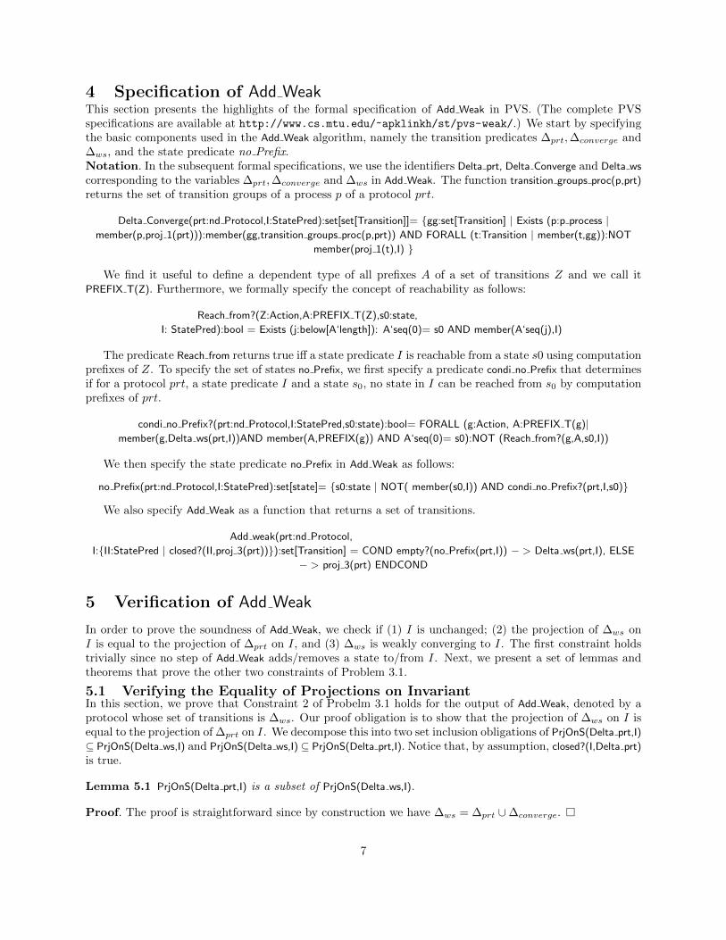
4 Specification of Add WeakThis section presents the highlights of the formal specification of Add Weak in PVS. (The complete PVSspecifications are available at http://www.cs.mtu.edu/~apklinkh/st/pvs-weak/.) We start by specifyingthe basic components used in the Add Weak algorithm, namely the transition predicates ∆prt,∆converge and∆ws, and the state predicate no Prefix.Notation. In the subsequent formal specifications, we use the identifiers Delta prt, Delta Converge and Delta ws

corresponding to the variables ∆prt,∆converge and ∆ws in Add Weak. The function transition groups proc(p,prt)

returns the set of transition groups of a process p of a protocol prt.

Delta Converge(prt:nd Protocol,I:StatePred):set[set[Transition]]= {gg:set[Transition] | Exists (p:p process |member(p,proj 1(prt))):member(gg,transition groups proc(p,prt)) AND FORALL (t:Transition | member(t,gg)):NOT

member(proj 1(t),I) }

We find it useful to define a dependent type of all prefixes A of a set of transitions Z and we call itPREFIX T(Z). Furthermore, we formally specify the concept of reachability as follows:

Reach from?(Z:Action,A:PREFIX T(Z),s0:state,

I: StatePred):bool = Exists (j:below[A‘length]): A‘seq(0)= s0 AND member(A‘seq(j),I)

The predicate Reach from returns true iff a state predicate I is reachable from a state s0 using computationprefixes of Z. To specify the set of states no Prefix, we first specify a predicate condi no Prefix that determinesif for a protocol prt, a state predicate I and a state s0, no state in I can be reached from s0 by computationprefixes of prt.

condi no Prefix?(prt:nd Protocol,I:StatePred,s0:state):bool= FORALL (g:Action, A:PREFIX T(g)|member(g,Delta ws(prt,I))AND member(A,PREFIX(g)) AND A‘seq(0)= s0):NOT (Reach from?(g,A,s0,I))

We then specify the state predicate no Prefix in Add Weak as follows:

no Prefix(prt:nd Protocol,I:StatePred):set[state]= {s0:state | NOT( member(s0,I)) AND condi no Prefix?(prt,I,s0)}

We also specify Add Weak as a function that returns a set of transitions.

Add weak(prt:nd Protocol,

I:{II:StatePred | closed?(II,proj 3(prt))}):set[Transition] = COND empty?(no Prefix(prt,I)) − > Delta ws(prt,I), ELSE

− > proj 3(prt) ENDCOND

5 Verification of Add Weak

In order to prove the soundness of Add Weak, we check if (1) I is unchanged; (2) the projection of ∆ws onI is equal to the projection of ∆prt on I, and (3) ∆ws is weakly converging to I. The first constraint holdstrivially since no step of Add Weak adds/removes a state to/from I. Next, we present a set of lemmas andtheorems that prove the other two constraints of Problem 3.1.

5.1 Verifying the Equality of Projections on InvariantIn this section, we prove that Constraint 2 of Probelm 3.1 holds for the output of Add Weak, denoted by aprotocol whose set of transitions is ∆ws. Our proof obligation is to show that the projection of ∆ws on I isequal to the projection of ∆prt on I. We decompose this into two set inclusion obligations of PrjOnS(Delta prt,I)

⊆ PrjOnS(Delta ws,I) and PrjOnS(Delta ws,I) ⊆ PrjOnS(Delta prt,I). Notice that, by assumption, closed?(I,Delta prt)

is true.

Lemma 5.1 PrjOnS(Delta prt,I) is a subset of PrjOnS(Delta ws,I).

Proof. The proof is straightforward since by construction we have ∆ws = ∆prt ∪∆converge. �

7

Lemma 5.2 PrjOnS(Delta ws,I) is a subset of PrjOnS(Delta prt,I).

Proof. If a transition t = (s0, s1) is in PrjOnS(Delta ws,I) then s0 ∈ I. Since ∆ws = ∆prt ∪∆converge, eithert ∈ ∆prt or t ∈ ∆converge. By construction, ∆converge excludes any transition starting in I including t. Thus,t must be in ∆prt. Since s0 ∈ I, it follows that t ∈ PrjOnS(Delta prt,I). �

Theorem 5.1 PrjOnS(Delta ws,I) = PrjOnS(Delta prt,I). (Proof follows from Lemmas 5.1 and 5.2.)

5.2 Verifying Weak Convergence

In this section, we prove the weak convergence property (i.e., Constraint 3 of Problem 3.1). Specifically, weshow that from any state s0 ∈ ¬I, there is a prefix A in PREFIX(Delta ws) such that A reaches some state inI. Again, we observe that, an underlying assumption in this section is that closed?(I,Delta prt) holds. For aprotocol prt and a predicate I that is closed in prt and a state s /∈ I, we have:

Lemma 5.3 If empty?(no Prefix(prt,I)) holds then condi no Prefix?(prt,I,s) returns false.

Lemma 5.4 If condi no Prefix?(prt,I,s) returns false, then there exists a sequence of states A and a set oftransitions Z such that Z ∈ Delta ws, A ∈ PREFIX(Z), A(0)=s holds, and Reach from?(Z,A,s,I) returns true.

Lemma 5.4 implies that when Add Weak returns, the revised version of prt guarantees that there exists acomputation prefix to I from any state outside I; hence weak convergence. This is due to the fact that A isa prefix of ∆ws.

Theorem 5.2 If empty?(no Prefix(prt,I)) holds and s /∈ I then there exists a sequence of states A that startsfrom s and A ∈ PREFIX(Delta ws) and Reach from?(Delta ws(prt,I),A,s,I) returns true.

Proof. Since the proof of this theorem is abstract, for ease of presentation we refer the reader to the proofof Theorem 7.1, which is an instantiation of this proof in the context of the token ring protocol. �

6 Compound Grind Proof Technique

This section presents a novel proof technique we use in proving the lemmas and theorems in our PVS theory.The contents of this section are orthogonal to the Add Weak PVS theory and can be applied for the proof oftheorems in different settings in PVS. We refer to the proposed technique as compound grind abbreviatedCOMP GRIND.

6.1 COMP GRIND Proof Technique

One reason behind the complexity of mechanical verification and deduction is that theorems and lemmasshould be proved interactively. This implies that the process of formalization has an experimental nature[32]. In particular, the choice of definitions and theorems must be performed very carefully; otherwise, themechanical verification may easily become unmanageable. For example, in PVS, the proof rule grind is verypowerful1. In many cases, grind can complete the proof. However, in some other cases (especially when theproof of a theorem requires long sequence of composite definitions and expansions) grind may fail to obtainthe correct instantiations or the definition expansions. Moreover, grind may lead to a large set of subgoalsdue to the fact that the proofs of subgoals were designed to be independent from each other. Next sectionprovides examples of the two cases.

Throughout our proof of Add Weak, we use a greedy algorithm to give a stable proof technique [9] to helpus detect the problematic formalizations. Further, to make the process more automated, we insert some

1The grind command can do skolemization, instantiation, if-lifting, proof simplification, rewriting using lemmas as rewriterules, definition expansion and explicit case analysis. grind can perform these steps repeatedly until no further simplificationis possible [34]

8

control points over the experimental nature of the mechanical proof process. In the proof of Add Weak, weuse the proposed method to create a reasonable number of subgoals/lemmas and to decrease the complexityof the used proof rules and strategies.

In order to prove implications of the form Q⇒ Z using the COMP GRIND method, we divide the proofinto a sequence of steps Q ⇒ a(1), Q ⇒ a(2), · · · , Q ⇒ a(n), where a(n) = Z. Each step is an implicationwith the antecedent Q and a different consequent a(i), where a(n) = Z. Moreover, each consequent a(i)should be specified in such a way that ∀i : 1 ≤ i < n : a(i)⇒ a(i+ 1) holds. We call this sequence the proofsequence of Q⇒ Z. Further, the following two conditions are met:

1. Let A(i) denote (Q ⇒ a(i)). The proof of A(i) should have at most c subgoals, where c is a fixednon-negative and small number. Otherwise, the formalization of Q ⇒ a(i) is considered problematicand we try to simplify it to meet this condition and Condition 2 below. If the reformulation techniquefails to decrease the number of subgoals, then we will divide A(i) into more than one node, where eachhas at most c subgoals. If that was impossible then the initial choice of c is updated and it becomesequal to the number of subgoals of A(i).

2. A(i) is proved by an appropriate instantiation for A(i−1) and a small number of simple rules less thanor equal to c in addition to grind.

In our experience c < 7 has worked well. Let R(i) denote the set of rules used in the proof of nodeA(i). Then, an element of R(i) can be (i) a simple primitive rule such as grind or Skosimp∗; (ii) a call to aprevious node, or an axiom. The cardinality of R(i) is less than or equal to c. There is a trade off betweenthe length of the proof sequence and the complexity of the proofs of the nodes. In the simplest non-trivialcase one can choose R to be {skosimp∗, grind}. However, we note that the efforts of formalizing a new nodeA(i) must not cost more than the efforts of completing the proof without A(i).

6.2 Recursive Nature of COMP GRIND

COMP GRIND has a bottom up recursive nature. In particular, for Q ⇒ Z, let lemma1 denote A(1).Consider the case where A(1) is proved by (skosimp∗, grind)). Then, the proof of lemma(2) = A(2) is asfollows:

(skosimp∗(node1(inst))), R(1), grind)

In general, the proof of node(n) which equals to Q⇒ Z can be represented by the following expression:

(skosimp∗(call(node(1, ..., n− 1)(inst))), grind,R(n− 1))

This recursive nature of COMP GRIND illustrates how proof efforts can be reused for proving higher-levellemmas/theorems.

6.3 Complexity of COMP GRIND

The actual cost of the proof of A(i) in terms of the number of proof rules is at most 2 + c plus the cost ofproving A(i − 1). (The constant 2 is due to using grind and skosimp.) Since PVS saves the proof of eachnode in a .prf file, invoking the saved proof has a unit cost. Thus, the worst case cost of proving A(i) wouldbe 2 + c+ (i− 1). Let n denote the length of the proof sequence. As a result, the worst case cost of proving

Q⇒ Z would be ((2 + c)× n) + (n2−n2 ) in terms of the number of proof rules, which would be O(n2). The

proof cost in terms of number of subgoals is at most c× n; i.e., O(n).

9

6.4 GRIND vs COMP GRIND

The objective of COMP GRIND is to control the behavior of grind towards avoiding a large number ofsubgoals. For example, the initial proof of the soundness of Add Weak required the proof of 90 subgoals,which was decreased to 4 subgoals after using the COMP GRIND technique. Even though the proofs ofsome nodes are non-trivial, COMP GRIND allows us to focus only on the proofs of the hardest parts of theoriginal proof tree. As a result, the focus of the prover shifts to the appropriate specification of each elementof the proof sequence.

7 Reusability and Generalizability

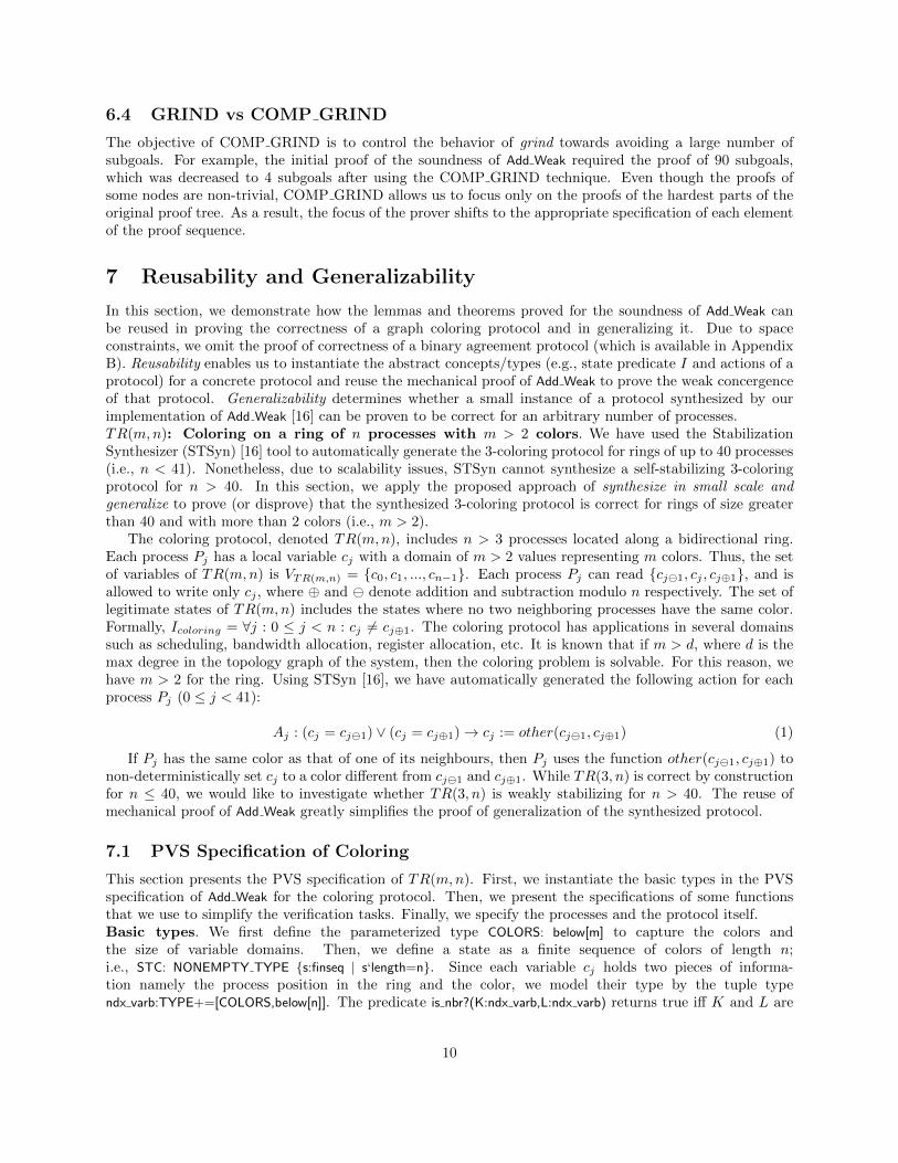
In this section, we demonstrate how the lemmas and theorems proved for the soundness of Add Weak canbe reused in proving the correctness of a graph coloring protocol and in generalizing it. Due to spaceconstraints, we omit the proof of correctness of a binary agreement protocol (which is available in AppendixB). Reusability enables us to instantiate the abstract concepts/types (e.g., state predicate I and actions of aprotocol) for a concrete protocol and reuse the mechanical proof of Add Weak to prove the weak concergenceof that protocol. Generalizability determines whether a small instance of a protocol synthesized by ourimplementation of Add Weak [16] can be proven to be correct for an arbitrary number of processes.TR(m,n): Coloring on a ring of n processes with m > 2 colors. We have used the StabilizationSynthesizer (STSyn) [16] tool to automatically generate the 3-coloring protocol for rings of up to 40 processes(i.e., n < 41). Nonetheless, due to scalability issues, STSyn cannot synthesize a self-stabilizing 3-coloringprotocol for n > 40. In this section, we apply the proposed approach of synthesize in small scale andgeneralize to prove (or disprove) that the synthesized 3-coloring protocol is correct for rings of size greaterthan 40 and with more than 2 colors (i.e., m > 2).

The coloring protocol, denoted TR(m,n), includes n > 3 processes located along a bidirectional ring.Each process Pj has a local variable cj with a domain of m > 2 values representing m colors. Thus, the setof variables of TR(m,n) is VTR(m,n) = {c0, c1, ..., cn−1}. Each process Pj can read {cj1, cj , cj⊕1}, and isallowed to write only cj , where ⊕ and denote addition and subtraction modulo n respectively. The set oflegitimate states of TR(m,n) includes the states where no two neighboring processes have the same color.Formally, Icoloring = ∀j : 0 ≤ j < n : cj 6= cj⊕1. The coloring protocol has applications in several domainssuch as scheduling, bandwidth allocation, register allocation, etc. It is known that if m > d, where d is themax degree in the topology graph of the system, then the coloring problem is solvable. For this reason, wehave m > 2 for the ring. Using STSyn [16], we have automatically generated the following action for eachprocess Pj (0 ≤ j < 41):

Aj : (cj = cj1) ∨ (cj = cj⊕1)→ cj := other(cj1, cj⊕1) (1)

If Pj has the same color as that of one of its neighbours, then Pj uses the function other(cj1, cj⊕1) tonon-deterministically set cj to a color different from cj1 and cj⊕1. While TR(3, n) is correct by constructionfor n ≤ 40, we would like to investigate whether TR(3, n) is weakly stabilizing for n > 40. The reuse ofmechanical proof of Add Weak greatly simplifies the proof of generalization of the synthesized protocol.

7.1 PVS Specification of Coloring

This section presents the PVS specification of TR(m,n). First, we instantiate the basic types in the PVSspecification of Add Weak for the coloring protocol. Then, we present the specifications of some functionsthat we use to simplify the verification tasks. Finally, we specify the processes and the protocol itself.Basic types. We first define the parameterized type COLORS: below[m] to capture the colors andthe size of variable domains. Then, we define a state as a finite sequence of colors of length n;i.e., STC: NONEMPTY TYPE {s:finseq | s‘length=n}. Since each variable cj holds two pieces of informa-tion namely the process position in the ring and the color, we model their type by the tuple typendx varb:TYPE+=[COLORS,below[n]]. The predicate is nbr?(K:ndx varb,L:ndx varb) returns true iff K and L are

10

two neighboring processes; i.e., mod(abs(K‘2-L‘2),n) ≤ 1, where K‘2 denotes the second element of the pair K(which is the position of K in the ring). Likewise, we define the predicate is bad nbr?(K:ndx varb,L:ndx varb)

that holds iff is nbr?(K,L) holds and K‘1 = L‘1. To capture the locality of process j, we define the non-empty dependent type nbr v(K:ndx varb):TYPE+ = {L:ndx varb | is nbr?(K,L) }. Likewise, we define the typebad nbr v(K:ndx varb):TYPE ={L:ndx varb | is bad nbr?(K,L)} to capture the set of neighbors of a process thathave the same color as that process. The function nbr colors(K:ndx varb):set[COLORS] returns the set of colorsof the immediate neighbours of a process.Functions. In order to simplify the verification of convergence (in Section 7.2), we associate the subsequentfunctions with a global state. For example, we define a function ValPos(s:STC,j:below[n]):ndx varb=(s‘seq(j),j)

that returns the value and the position of process j in a global state s as a tuple of type ndx varb.An example use of this function is Val(s:STC,L:ndx varb)= ValPos(s,L‘2)‘1. Moreover, the predicatenbr is bad?(s:STC,j:below[n]):bool = nonempty?(bad nbr v(ValPos(s,j))) returns true iff for an arbitrary state sand a process j the set of bad neighbors of the variable ValPos(s,j) is nonempty; we refer to such a caseby saying s is corrupted at process j. Notice that an illegitimate state can be corrupted at more thanone position. We also define the predicate nbr is good?(s:STC,j:below[n]):bool as the negation of the predicatenbr is bad?(s:STC,j:below[n]):bool. Using the aforementioned functions, we also define the set of illegitimatestates as S ill:TYPE= { s:STC | not is LEGT?(s)}, where is LEGT?(s:STC):bool= Forall (j:below[n]): nbr is good?(s,j).The association of a global state to functions and types enables us to import Add Weak Conv theory withthe following types [STC,below[m], ndx varb, [ndx varb, STC → below[m]]] to reuse its already defined types andfunctions in specifying TR(m,n) as follows.Specification of a process of TR(m,n). For an arbitrary global state s and a process j, we define thefunction READ p which returns all readable variables of process j.

READ p(s:STC, j:below[n]): set[ndx varb]= {L:nbr v(ValPos(s,j)) | TRUE } .Similarly, we define the function WRITE p which returns the variables that process j can write.WRITE p(s:STC,j:below[n]): set[ndx varb]= {L:ndx varb | L = ValPos(s,j)}We now define the action of a process j as a function that returns the set of transitions belonging to that

action.DELTA p(s:STC,j:below[n]):set[Transition] ={tr: Transition | Exists (c:bad nbr v(ValPos(s,j))): tr =

(s,action(s,j,ValPos(s,j),c)) }Intuitively, the function DELTA p returns the set of transitions that belong to process j if process j is

corrupted in the global state s; i.e., j has a bad neighbor. The function action(s,j,ValPos(s,j),c) returns thestate reached when process j acts to correct its corrupted state. Formally, we define action(s,j,ValPos(s,j),c) asfollows: (The LAMBDA abstractions in PVS enable us to specify binding expressions similar to quantifiedstatements in predicate logic. )

action(s:STC,j:below[n],K:ndx varb, C:bad nbr v(K)): STC = (# length := n, seq := (LAMBDA (i:below[n]):IF i= j

THEN other(ValPos(s,j)) ELSE s(i) ENDIF) #)

We specify the function other to randomly choose a new color other than the corrupted one. To thisend, we use the epsilon function over the full set of colors minus the set of colors of the neighbors of thecorrupted process. Formally, we have other(K:ndx varb):COLORS = epsilon(difference(fullset colors,nbr colors(K))

), where fullset colors:set[COLORS]= {cl:COLORS | TRUE}. We now present the specification of a process of theprotocol TR(m,n).

PRS p(s:STC,j:below[n]): p process = (READ p(s,j), WRITE p(s,j),DELTA p(s,j))

The parameterized specification of the TR(m,n) protocol. We define the TR(m,n) protocol as thetype TR m n(s:STC):nd Protocol =(PROC prt(s),VARB prt(s),DELTA prt(s) ), where the parameters are defined asfollows:

PROC prt(s:STC): set[p process]={p:p process | Exists (j:below[n]):p = PRS p(s,j)}VARB prt(s:STC): set[ndx varb]= {v:ndx varb | Exists (j:below[n]):member(v, WRITE p(s,j) )}Delta prt(s:STC): set[Transition]= {tr:Transition | Exists (j:below[n]):member(tr,DELTA p(s,j))} .

11

7.2 Mechanical Verification of Parameterized Coloring

We now prove the weak convergence of TR(m,n) for m > 2 and n > 40. To this end, we show that the setno Prefix of TR(m,n) is actually empty. The proof of emptiness of no Prefix is based on a prefix constructorfunction that demonstrates the existence of a computation prefix σ of TR(m,n) from any arbitrary illegit-imate state s such that σ includes a state in I. Subsequently, we instantiate Theorem 5.2 for TR(m,n).Please see the Appendix A for the details of the proof.

Theorem 7.1 Let prt be TR(m,n). If closed?(I,(prt)‘3) and empty?(no Prefix(prt,I)) hold and s /∈ I then thereexists a sequence of states A that starts from s and A ∈ PREFIX(Delta ws(prt,I)) and Reach from?(A,s,I) returnstrue.

Proof. We show that Add Weak will generate a weakly stabilizing version of protocol TR(m,n) for any n > 3and m > 2. To this end, we show that TR(m,n) has an empty no Prefix set and instantiate Theorem 5.2 forTR(m,n).Emptiness of no PREFIX for TR(m,n). To prove the weak convergence of TR(m,n), we show that theset no Prefix of TR(m,n) is empty. Let s be an arbitrary illegitimate state. We define a sequence of states σthat starts in s and terminates in I such that all transitions of σ belong to proj 3(TR(m,n)). Before buildinga prefix from a particular illegitimate state s, we would like to identify a segment of the ring that is correctin the sense that the local predicate ((ci 6= ci−1) ∧ (ci 6= ci+1)) is correct for processes from 1 to j; i.e.,∀i : 1 ≤ i ≤ j : ((ci 6= ci−1) ∧ (ci 6= ci+1)). For this purpose, we define three auxiliary functions. The firstone is a corrector function that applies the other function on ValPos(s,j) if process j is corrupted; otherwise,it leaves cj as is.

corrector(s:S ill, j:below[n]):COLORS = COND nbr is good?(s,j) → s‘seq(j), nbr is bad?(s,j) → other(ValPos(s,j))

ENDCOND

sc(s:S ill,j:below[n]):STC= (# length := n, seq := (LAMBDA (i:below[n]):IF i ≤ j THEN corrector(s,i) ELSE s‘seq(i)

ENDIF) #)

The function sc(s,j) takes an illegitimate state s and an index j of the ring, and returns a global state whereall processes from 1 to j have good neighbors. The rest of the processes have the same state as in s. Since wemodel a global state of a ring of n processes as a sequence of n colors, we can represent the application of the sc

function on the j-th process in a global state s (denoted sc(s,j)) as 〈 corrector(s,0),...,corrector(s,j),s(j+1),...,s(n-1))

〉, where the colors of processes from j + 1 to n− 1 remain unchanged by sc.The function AA below is especially useful because constructing the appropriate computation prefix from

s to some invariant state in I directly is not straightforward. Since for all j < n we do not know whetherapplying the corrector function on a state s:S ill at a process j will result in a legitimate state, we use AA tobuild a sequence of states of length n formed by applying the corrector function consecutively at all processesregardless of being corrupted or not.

AA(s:S ill): Pos F S = (# length := n, seq := (LAMBDA (i:below[n]): sc(s,i) ) #)

Each element j in the sequence that AA(s) returns is the image of the function sc(s,j), which is a statethat is correct up to process j. We define the function min lgt(AA(s)) over the sequence AA(s) to return theminimum index for which the corresponding state is legitimate.

lgtStatesIndices(A:Pos F S):set[below[A‘length]]={i:below[A‘length] | is LEGT?(A‘seq(i)) }min Index(A:Pos F S):{i:integer | i≥-1} = COND not empty?(lgtStatesIndices(A)) − > min(lgtStatesIndices(A)), else

− > -1 ENDCOND

The Prefix-Constructor function. Now we are ready to define the constructor function of the requiredprefix from any s:S ill to I as follows:

constPrefix(s:S ill):Pos F S = (# length:= min Index(AA(s))+2, seq:= (LAMBDA (i:below[min Index(AA(s))+2]): if

i=0 then s else sc(s,i-1) endif) #)

The last element of constPrefix(s) is the first legitimate state of AA(s). Thus, all states before the laststate in constPrefix(s) are illegitimate. Moreover, each application of the corrector function corresponds toa transition that starts in an illegitimate state. This is true until reaching a legitimate state. Thus, allinvolved transitions in the sequence AA(s) are in TR(m,n), thereby making constPrefix(s) a computationprefix of TR(m,n). To show the correctness of this argument, it is sufficient to show the existence of at

12

least one index that is equal to min lgt(AA(s)). Thus, the sequence constPrefix(s) is well-defined for any states outside I and reaches I as required. Thus, it is sufficient for weak convergence to show the correctness ofthe following two properties of the function sc.

1. If a process j is corrupted then the color of process j in the state sc(s,n-1) is the same as what thecorrector function selects for it; i.e., ValPos(sc(s,n-1), j)‘1= other(ValPos(s,j)).

2. If a process j is corrupted then in the state sc(s,n-1) the process j is not corrupted (i.e., does not havea corrupted neighbor as well).

Notice that by the above two properties we show that the state generated by sc(s,n-1) is legitimate. Weprove these properties as two lemmas.

Lemma 7.1 If nonempty?(bad nbr s(ValPos(s,j))) holds then ValPos(sc(s,n-1), j)‘1 = other(ValPos(s,j)).

Lemma 7.2 If nonempty?(bad nbr s(ValPos(s,j))) holds then empty?(bad nbr s((other(ValPos(s,j)), j))).

The mechanical proofs of these lemmas follow directly by expanding the required definitions and usingthe following axiom of choice.

AXIOM nonempty?(bad nbr s(ValPos(sl,j))) IMPLIES empty?(C: ndx varb | is bad nbr?((other(ValPos(sl, j)), j), C))

We need the axiom of choice because we use the epsilon function in the definition of the other() function.This way we show there is always a different color that can correct the locality of a corrupted process.

Theorem 7.2 Let prt be TR(m,n). If closed?(I,(prt)‘3) and empty?(no Prefix(prt,I)) hold and s /∈ I then thereexists a sequence of states A that starts from s and A ∈ PREFIX(Delta ws(prt,I)) and Reach from?(A,s,I) returnstrue.

8 Verifying the Convergence of Binary Agreement (AG)

In this section, we prove two correctness properties of any instance of the AG protocol using PVS. First,we verify that any synthesized version of AG generated by the Add Weak algorithm is weakly stabilizing.Second, the small synthesized AG protocol in [6] is weakly stabilizing for any n >= 3; i.e., the protocol in[6] is generalizability.Example. The protocol AG(n) includes n > 2 processes located on a unidirectional ring. Each process pj hasa variable cj with a domain Dom = {0, 1}. Thus, AG(n) has the set of variables VAG(n) = {c0, c1, ..., cn−1}.Each process can read but not write its left neighbor; i.e., Readp = {cj1, cj} while Writep = {cj}. Eachprocess has an action defined by :

Aj : cj1 < cj → cj := cj1 (2)

If the variable cj has a value greater than its predecessor then the process pj sets the value of cj to cj1(which is equal to 0 due to the binary domain).

A legitimate state of the AG(n) protocol is a state where all variables have the same value. If the condition(cj1 < cj) holds for a process j, then we call it a locally corrupted process; otherwise, we say the protocolis silent at process j.

8.1 PVS Specification of AG(n)

In our PVS specification of AG(n) there are n processes, where n is a theory parameter of type posnatfor the model. We assume that n > 2. We define the type Bin : below[2] to capture the domain ofthe variables. Moreover, we formalize a global state of AG(n) as a finite binary sequence of length n;i.e., STC : NONEMPTY TY PE{s : finseq(Bin) | s‘length = n}. Furthermore, since each variablecj has two pieces of information namely the process position and its value, we model its type by a tuplendx varb : TY PE+ = [Bin, below[n]].

13

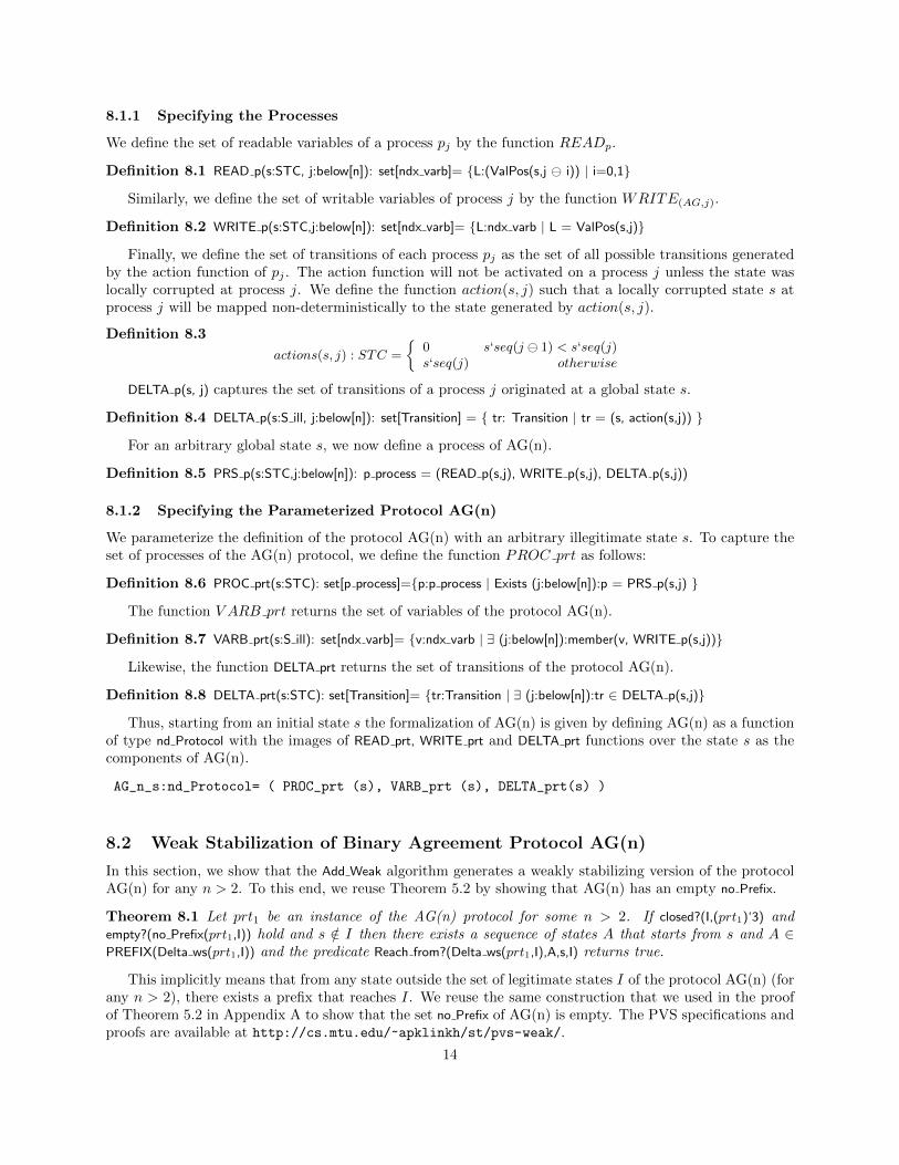
8.1.1 Specifying the Processes

We define the set of readable variables of a process pj by the function READp.

Definition 8.1 READ p(s:STC, j:below[n]): set[ndx varb]= {L:(ValPos(s,j i)) | i=0,1}

Similarly, we define the set of writable variables of process j by the function WRITE(AG,j).

Definition 8.2 WRITE p(s:STC,j:below[n]): set[ndx varb]= {L:ndx varb | L = ValPos(s,j)}

Finally, we define the set of transitions of each process pj as the set of all possible transitions generatedby the action function of pj . The action function will not be activated on a process j unless the state waslocally corrupted at process j. We define the function action(s, j) such that a locally corrupted state s atprocess j will be mapped non-deterministically to the state generated by action(s, j).

Definition 8.3

actions(s, j) : STC =

{0 s‘seq(j 1) < s‘seq(j)s‘seq(j) otherwise

DELTA p(s, j) captures the set of transitions of a process j originated at a global state s.

Definition 8.4 DELTA p(s:S ill, j:below[n]): set[Transition] = { tr: Transition | tr = (s, action(s,j)) }

For an arbitrary global state s, we now define a process of AG(n).

Definition 8.5 PRS p(s:STC,j:below[n]): p process = (READ p(s,j), WRITE p(s,j), DELTA p(s,j))

8.1.2 Specifying the Parameterized Protocol AG(n)

We parameterize the definition of the protocol AG(n) with an arbitrary illegitimate state s. To capture theset of processes of the AG(n) protocol, we define the function PROC prt as follows:

Definition 8.6 PROC prt(s:STC): set[p process]={p:p process | Exists (j:below[n]):p = PRS p(s,j) }

The function V ARB prt returns the set of variables of the protocol AG(n).

Definition 8.7 VARB prt(s:S ill): set[ndx varb]= {v:ndx varb | ∃ (j:below[n]):member(v, WRITE p(s,j))}

Likewise, the function DELTA prt returns the set of transitions of the protocol AG(n).

Definition 8.8 DELTA prt(s:STC): set[Transition]= {tr:Transition | ∃ (j:below[n]):tr ∈ DELTA p(s,j)}

Thus, starting from an initial state s the formalization of AG(n) is given by defining AG(n) as a functionof type nd Protocol with the images of READ prt, WRITE prt and DELTA prt functions over the state s as thecomponents of AG(n).

AG_n_s:nd_Protocol= ( PROC_prt (s), VARB_prt (s), DELTA_prt(s) )

8.2 Weak Stabilization of Binary Agreement Protocol AG(n)

In this section, we show that the Add Weak algorithm generates a weakly stabilizing version of the protocolAG(n) for any n > 2. To this end, we reuse Theorem 5.2 by showing that AG(n) has an empty no Prefix.

Theorem 8.1 Let prt1 be an instance of the AG(n) protocol for some n > 2. If closed?(I,(prt1)‘3) andempty?(no Prefix(prt1,I)) hold and s /∈ I then there exists a sequence of states A that starts from s and A ∈PREFIX(Delta ws(prt1,I)) and the predicate Reach from?(Delta ws(prt1,I),A,s,I) returns true.

This implicitly means that from any state outside the set of legitimate states I of the protocol AG(n) (forany n > 2), there exists a prefix that reaches I. We reuse the same construction that we used in the proofof Theorem 5.2 in Appendix A to show that the set no Prefix of AG(n) is empty. The PVS specifications andproofs are available at http://cs.mtu.edu/~apklinkh/st/pvs-weak/.

14

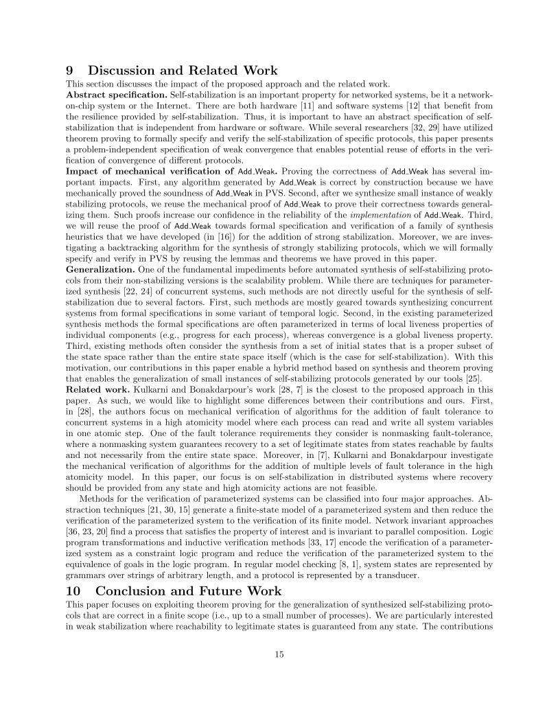
9 Discussion and Related WorkThis section discusses the impact of the proposed approach and the related work.Abstract specification. Self-stabilization is an important property for networked systems, be it a network-on-chip system or the Internet. There are both hardware [11] and software systems [12] that benefit fromthe resilience provided by self-stabilization. Thus, it is important to have an abstract specification of self-stabilization that is independent from hardware or software. While several researchers [32, 29] have utilizedtheorem proving to formally specify and verify the self-stabilization of specific protocols, this paper presentsa problem-independent specification of weak convergence that enables potential reuse of efforts in the veri-fication of convergence of different protocols.Impact of mechanical verification of Add Weak. Proving the correctness of Add Weak has several im-portant impacts. First, any algorithm generated by Add Weak is correct by construction because we havemechanically proved the soundness of Add Weak in PVS. Second, after we synthesize small instance of weaklystabilizing protocols, we reuse the mechanical proof of Add Weak to prove their correctness towards general-izing them. Such proofs increase our confidence in the reliability of the implementation of Add Weak. Third,we will reuse the proof of Add Weak towards formal specification and verification of a family of synthesisheuristics that we have developed (in [16]) for the addition of strong stabilization. Moreover, we are inves-tigating a backtracking algorithm for the synthesis of strongly stabilizing protocols, which we will formallyspecify and verify in PVS by reusing the lemmas and theorems we have proved in this paper.Generalization. One of the fundamental impediments before automated synthesis of self-stabilizing proto-cols from their non-stabilizing versions is the scalability problem. While there are techniques for parameter-ized synthesis [22, 24] of concurrent systems, such methods are not directly useful for the synthesis of self-stabilization due to several factors. First, such methods are mostly geared towards synthesizing concurrentsystems from formal specifications in some variant of temporal logic. Second, in the existing parameterizedsynthesis methods the formal specifications are often parameterized in terms of local liveness properties ofindividual components (e.g., progress for each process), whereas convergence is a global liveness property.Third, existing methods often consider the synthesis from a set of initial states that is a proper subset ofthe state space rather than the entire state space itself (which is the case for self-stabilization). With thismotivation, our contributions in this paper enable a hybrid method based on synthesis and theorem provingthat enables the generalization of small instances of self-stabilizing protocols generated by our tools [25].Related work. Kulkarni and Bonakdarpour’s work [28, 7] is the closest to the proposed approach in thispaper. As such, we would like to highlight some differences between their contributions and ours. First,in [28], the authors focus on mechanical verification of algorithms for the addition of fault tolerance toconcurrent systems in a high atomicity model where each process can read and write all system variablesin one atomic step. One of the fault tolerance requirements they consider is nonmasking fault-tolerance,where a nonmasking system guarantees recovery to a set of legitimate states from states reachable by faultsand not necessarily from the entire state space. Moreover, in [7], Kulkarni and Bonakdarpour investigatethe mechanical verification of algorithms for the addition of multiple levels of fault tolerance in the highatomicity model. In this paper, our focus is on self-stabilization in distributed systems where recoveryshould be provided from any state and high atomicity actions are not feasible.

Methods for the verification of parameterized systems can be classified into four major approaches. Ab-straction techniques [21, 30, 15] generate a finite-state model of a parameterized system and then reduce theverification of the parameterized system to the verification of its finite model. Network invariant approaches[36, 23, 20] find a process that satisfies the property of interest and is invariant to parallel composition. Logicprogram transformations and inductive verification methods [33, 17] encode the verification of a parameter-ized system as a constraint logic program and reduce the verification of the parameterized system to theequivalence of goals in the logic program. In regular model checking [8, 1], system states are represented bygrammars over strings of arbitrary length, and a protocol is represented by a transducer.

10 Conclusion and Future WorkThis paper focuses on exploiting theorem proving for the generalization of synthesized self-stabilizing proto-cols that are correct in a finite scope (i.e., up to a small number of processes). We are particularly interestedin weak stabilization where reachability to legitimate states is guaranteed from any state. The contributions

15

of this paper comprise a component of a hybrid method for verification and synthesis of parameterized self-stabilizing network protocols (see Figure 1). Previous work [13, 16] provides algorithmic methods that takea small instance of a non-stabilizing protocol and automatically generates a self-stabilizing version thereof.This paper specifically presents a mechanical proof for the correctness of the Add Weak algorithm from [16]that synthesizes weak convergence. This mechanical proof provides a reusable theory in PVS for the proof ofweakly stabilizing systems in general (irrespective of how they have been designed). The success of mechnicalproof for a small synthesized protocol shows the generality of the synthesized solution for arbitrary numberof processes. We have demonstrated the proposed approach in the context of a binary agreement protocol(Appendix B) and a graph coloring procotol (Section 7).

We will extend this work by reusing the existing PVS theory for mechanical proof of algorithms (in[16]) that design strong convergence. Moreover, we are currently investigating the generalization of morecomplicated protocols (e.g., leader election, maximal matching, consensus) using the proposed approach.

References

[1] P. A. Abdulla, B. Jonsson, M. Nilsson, and M. Saksena. A survey of regular model checking. InCONCUR, pages 35–48, 2004.

[2] F. Abujarad and S. S. Kulkarni. Multicore constraint-based automated stabilization. In 11th Interna-tional Symposium on Stabilization, Safety, and Security of Distributed Systems, pages 47–61, 2009.

[3] F. Abujarad and S. S. Kulkarni. Automated constraint-based addition of nonmasking and stabilizingfault-tolerance. Theoretical Computer Science, 412(33):4228–4246, 2011.

[4] A. Arora and M. G. Gouda. Closure and convergence: A foundation of fault-tolerant computing. IEEETransactions on Software Engineering, 19(11):1015–1027, 1993.

[5] P. C. Attie, anish Arora, and E. A. Emerson. Synthesis of fault-tolerant concurrent programs. ACMTransactions on Programming Languages and Systems (TOPLAS), 26(1):125–185, 2004.

[6] B. Bonakdarpour, A. Ebnenasir, and S. S. Kulkarni. Complexity results in revising UNITY programs.ACM Transactions on Autonomous and Adaptive Systems, 4(1):2009, 1–28.

[7] B. Bonakdarpour and S. S. Kulkarni. Towards reusing formal proofs for verification of fault-tolerance.In Workshop in Automated Formal Methods, 2006.

[8] A. Bouajjani, B. Jonsson, M. Nilsson, and T. Touili. Regular model checking. In CAV, pages 403–418,2000.

[9] E. Denney, J. Power, and K. Tourlas. Hiproofs: A hierarchical notion of proof tree. Electr. Notes Theor.Comput. Sci., 155:341–359, 2006.

[10] E. W. Dijkstra. Self-stabilizing systems in spite of distributed control. Communications of the ACM,17(11):643–644, 1974.

[11] S. Dolev and Y. A. Haviv. Self-stabilizing microprocessor: analyzing and overcoming soft errors. Com-puters, IEEE Transactions on, 55(4):385–399, 2006.

[12] S. Dolev and R. Yagel. Self-stabilizing operating systems. In Proceedings of the twentieth ACM sympo-sium on Operating systems principles, pages 1–2. ACM, 2005.

[13] A. Ebnenasir and A. Farahat. Swarm synthesis of convergence for symmetric protocols. In Proceedingsof the Ninth European Dependable Computing Conference, pages 13–24, 2012.

[14] A. Ebnenasir, S. S. Kulkarni, and A. Arora. FTSyn: A framework for automatic synthesis of fault-tolerance. International Journal on Software Tools for Technology Transfer, 10(5):455–471, 2008.

16

[15] E. A. Emerson and K. S. Namjoshi. On reasoning about rings. International Journal of Foundationsof Computer Science, 14(4):527–550, 2003.

[16] A. Farahat and A. Ebnenasir. A lightweight method for automated design of convergence in networkprotocols. ACM Transactions on Autonomous and Adaptive Systems (TAAS), 7(4):38:1–38:36, Dec.2012.

[17] F. Fioravanti, A. Pettorossi, M. Proietti, and V. Senni. Generalization strategies for the verification ofinfinite state systems. TPLP, 13(2):175–199, 2013.

[18] M. J. C. Gordon and T. F. Melham. Introduction to HOL: A Theorem proving Environment for HigherOrder Logic. Cambridge University Press, 1993.

[19] M. Gouda. The theory of weak stabilization. In 5th International Workshop on Self-Stabilizing Systems,volume 2194 of Lecture Notes in Computer Science, pages 114–123, 2001.

[20] O. Grinchtein, M. Leucker, and N. Piterman. Inferring network invariants automatically. In AutomatedReasoning, pages 483–497. Springer, 2006.

[21] C. N. Ip and D. L. Dill. Verifying systems with replicated components in murphi. Formal Methods inSystem Design, 14(3):273–310, 1999.

[22] S. Jacobs and R. Bloem. Parameterized synthesis. In International Conference on Tools and Algorithmsfor the Construction and Analysis of Systems (TACAS), pages 362–376, 2012.

[23] Y. Kesten, A. Pnueli, E. Shahar, and L. Zuck. Network invariants in action*. In CONCUR 2002Con-currency Theory, pages 101–115. Springer, 2002.

[24] A. Khalimov, S. Jacobs, and R. Bloem. Party parameterized synthesis of token rings. In ComputerAided Verification, pages 928–933. Springer, 2013.

[25] A. Klinkhamer and A. Ebnenasir. An embarrassingly parallel tool for automated synthesis of self-stabilization. http://www.cs.mtu.edu/~apklinkh/protocon/index.html.

[26] A. Klinkhamer and A. Ebnenasir. On the complexity of adding convergence. In Proceedings of the 5thInternational Symposium on Fundamentals of Software Engineering (FSEN), pages 17–33, 2013.

[27] S. S. Kulkarni and A. Arora. Automating the addition of fault-tolerance. In Formal Techniques inReal-Time and Fault-Tolerant Systems, pages 82–93, London, UK, 2000. Springer-Verlag.

[28] S. S. Kulkarni, B. Bonakdarpour, and A. Ebnenasir. Mechanical verification of automatic synthesisof fault-tolerance. International Symposium on Logic-based Program Synthesis and Transformation(LOPSTR), in Lecture Notes in Computer Science, 3573:36–52, 2004.

[29] S. S. Kulkarni, J. Rushby, and N. Shankar. A case-study in component-based mechanical verificationof fault-tolerant programs. In 19th IEEE International Conference on Distributed Computing Systems- Workshop on Self-Stabilizing Systems, pages 33–40, 1999.

[30] A. Pnueli, J. Xu, and L. D. Zuck. Liveness with (0, 1, infty)-counter abstraction. In InternationalConference on Computer Aided Verification (CAV), pages 107–122, 2002.

[31] I. S. W. B. Prasetya. Mechanically verified self-stabilizing hierarchical algorithms. Tools and Algorithmsfor the Construction and Analysis of Systems (TACAS’97), volume 1217 of Lecture Notes in ComputerScience, pages 399–415, 1997.

[32] S. Qadeer and N. Shankar. Verifying a self-stabilizing mutual exclusion algorithm. In D. Gries andW.-P. de Roever, editors, IFIP International Conference on Programming Concepts and Methods (PRO-COMET ’98), pages 424–443, Shelter Island, NY, June 1998. Chapman & Hall.

17

[33] A. Roychoudhury, K. N. Kumar, C. Ramakrishnan, I. Ramakrishnan, and S. A. Smolka. Verifica-tion of parameterized systems using logic program transformations. In Tools and Algorithms for theConstruction and Analysis of Systems, pages 172–187. Springer, 2000.

[34] N. Shankar, S. Owre, and J. M. Rushby. The PVS Proof Checker: A Reference Manual. ComputerScience Laboratory, SRI International, Menlo Park, CA, Feb. 1993. A new edition for PVS Version 2 isreleased in 1998.

[35] T. Tsuchiya, S. Nagano, R. B. Paidi, and T. Kikuno. Symbolic model checking for self-stabilizingalgorithms. IEEE Transactions on Parallel and Distributed Systems, 12(1):81–95, 2001.

[36] P. Wolper and V. Lovinfosse. Verifying properties of large sets of processes with network invariants.In International Workshop on Automatic Verification Methods for Finite State Systems, pages 68–80,1989.

18