Computer Science & Information Technology (CS & IT)
105
Computer Science & Information Technology 138
Transcript of Computer Science & Information Technology (CS & IT)

Computer Science & Information Technology 138


David C. Wyld,
Dhinaharan Nagamalai (Eds)
Computer Science & Information Technology
10th International Conference on Software Engineering and Applications (SEAS 2021),
February 20~21, 2021, Dubai, UAE.
AIRCC Publishing Corporation

Volume Editors
David C. Wyld,
Southeastern Louisiana University, USA
E-mail: [email protected]
Dhinaharan Nagamalai (Eds),
Wireilla Net Solutions, Australia
E-mail: [email protected]
ISSN: 2231 - 5403 ISBN: 978-1-925953-36-7
DOI: 10.5121/csit.2021.110201- 10.5121/csit.2021.110205
This work is subject to copyright. All rights are reserved, whether whole or part of the material is concerned, specifically the rights of translation, reprinting, re-use of illustrations, recitation,
broadcasting, reproduction on microfilms or in any other way, and storage in data banks.
Duplication of this publication or parts thereof is permitted only under the provisions of the
International Copyright Law and permission for use must always be obtained from Academy & Industry Research Collaboration Center. Violations a reliable to prosecution under the
International Copyright Law.
Typesetting: Camera-ready by author, data conversion by NnN Net Solutions Private Ltd.,
Chennai, India

Preface
The 10th International Conference on Software Engineering and Applications (SEAS 2021), February 20~21, 2021, Dubai, UAE and 10th International Conference on Control, Modelling,
Computing and Applications (CMCA 2021) and 8th International Conference on Advanced
Computing (ADCO 2021) was collocated with 10th International Conference on Software
Engineering and Applications (SEAS 2021). The conferences attracted many local and international delegates, presenting a balanced mixture of intellect from the East and from the
West.
The goal of this conference series is to bring together researchers and practitioners from academia and industry to focus on understanding computer science and information technology
and to establish new collaborations in these areas. Authors are invited to contribute to the
conference by submitting articles that illustrate research results, projects, survey work and
industrial experiences describing significant advances in all areas of computer science and information technology.
The SEAS 2021, CMCA 2021 and ADCO 2021 Committees rigorously invited submissions for
many months from researchers, scientists, engineers, students and practitioners related to the relevant themes and tracks of the workshop. This effort guaranteed submissions from an
unparalleled number of internationally recognized top-level researchers. All the submissions
underwent a strenuous peer review process which comprised expert reviewers. These reviewers
were selected from a talented pool of Technical Committee members and external reviewers on the basis of their expertise. The papers were then reviewed based on their contributions, technical
content, originality and clarity. The entire process, which includes the submission, review and
acceptance processes, was done electronically.
In closing, SEAS 2021, CMCA 2021 and ADCO 2021 brought together researchers, scientists, engineers, students and practitioners to exchange and share their experiences, new ideas and
research results in all aspects of the main workshop themes and tracks, and to discuss the
practical challenges encountered and the solutions adopted. The book is organized as a collection of papers from the SEAS 2021, CMCA 2021 and ADCO 2021.
We would like to thank the General and Program Chairs, organization staff, the members of the
Technical Program Committees and external reviewers for their excellent and tireless work. We
sincerely wish that all attendees benefited scientifically from the conference and wish them every success in their research. It is the humble wish of the conference organizers that the professional
dialogue among the researchers, scientists, engineers, students and educators continues beyond
the event and that the friendships and collaborations forged will linger and prosper for many years to come.
David C. Wyld,
Dhinaharan Nagamalai (Eds)

General Chair Organization David C. Wyld, Jackson State University, USA
Dhinaharan Nagamalai(Eds) Wireilla Net Solutions, Australia
Program Committee Members
Abdessamad Belangour, University Hassan Ii Casablanca, Morocco
Abdolreza Hatamlou, Islamic Azad University, Iran
Adriana Carla, Federal University of Campina Grande (UFCG), Brazil Afaq Ahmad, Sultan Qaboos University, Oman
Ahmad Fakharian, Islamic Azad University, Iran
Ahmad Khasawneh, Irbid National University, Jordan Ahmed A. Elngar, Beni-Suef University, Egypt
Ahmed Korichi, University Of Ouargla, Algeria
Ajay Anil Gurjar, Sipna College of Engineering & Technology, India
Akhil Gupta, Lovely Professional University, India Ali Asghar Rahmani Hosseinabadi, Islamic Azad University, Iran
Amal Azeroual, Mohammed V University, Morocco
Amel Ourici, University Badji Mokhtar Annaba, Algeria Anas M.R. Al Sobeh, Yarmouk University, Jordan
Anirban Banik, National Institute of Technology Agartala, India
Ansar Daghouri, University Hassan Ii of Casablanca, Morocco Arianit Maraj, Aab College, Republic Of Kosovo
Asif Irshad Khan, King Abdulaziz University, Saudi Arabia
Aubrun, Christophe University of Lorraine, France
Ayad Salhieh, Australian College of Kuwait (Ack), Kuwait Benaddy Mohamed, Ibn Zohr University, Morocco
Berenguel, Manuel Universidad de Almeria, Spain
Blasco, Xavier Universitat Politécnica de Valencia, Spain Bogdan, Stjepan Univ. of Zagreb, Croatia
Bokor, Jozsef Hungarian Academic of Sciences, Hungary
Bouhorma Mohammed, Fstt, Morocco
Boukari Nassim, Skikda University, Algeria Bucher, Roberto Scuola Univ. Professionale, Switzerland
Camacho, Eduardo F. Universidad de Sevilla, Spain
Celia Ghedini Ralha, University of Brasalia (Unb), Brazil Chien-Cheng Yu, Hsiuping University of Science and Technology, Taiwan
Ching-Nung Yang, National Dong Hwa University, Taiwan
Claudio Schifanella, University Of Turin, Italy Dariusz Jakóbczak, Koszalin University of Technology, Poland
Dhanya Jothimani, Ryerson University, Canada
Dimitris Kanellopoulos, University of Patras, Greece
Ding Wang, Nankai University, China Djamel Eddine, University Of Biskra, Algeria
Elhabil Brahim, Ibn Zohr University, Morocco
El-Sayed M. El-Horbaty, Ain Shams University, Egypt Emad Awada, Applied Science University, Jordan
Emma Moupojou, University Of Yaounde, Cameroon

Erdal Ozdogan, Gazi University, Turkey Esmaiel Nojavani, University Of Isfahan, Iran
Faeq A.A.Radwan, Near East University, Turkey
Fazlollah Abbasi, Islamic Azad University, Iran
Fei Hui, Chang'an University, P.R.China Felix J. Garcia Clemente, University Of Murcia, Spain
Froilan Mobo, Merchant Marine Academy, Philippines
Gajendra Sharma, Kathmandu University, Nepal Gurkana, Yildiz Technical University, Turkey
Gururaj H L, Vidyavardhaka College of Engineering, India
Haider M. Alsabbagh, University Of Basrah, Iraq Haitham J.Taha, University Of Technology, Iraq
Hamid Alasadi, Basra University, Iraq
Hamid Ali Abed AL-Asadi, Iraq University College, Iraq
Hayet Mouss, Batna Univeristy, Algeria Hongzhi, Harbin Institute of Technology, China
Iyad Alazzam, Yarmouk University, Jordan
Jalel Akaichi, University of Tunis, Tunisia Kamel Hussein Rahouma, Minia University, Egypt
Kenjiro T. Miura, Shizuoka University, Japan
Mahdi Abbasi, Bu-Ali Sina University, Iran Mallikharjuna Rao K, VIT-AP University, India
Merniz Salah, University of Constantine 2, Algeria
Metasebia Alemante, ZTE University, China
Mohammad Al_Selam, University of Technology, Iraq Mohammed Bouhorma, FST of Tangier, Morocco
Muhammad Sarfraz, Kuwait University, Kuwait
Nalini Chidambaram, Bharath University, India Narasimham Challa, SR Engineering College, India
Neda Darvish, Islamic Azad University, Iran
Osama Rababah, University of Jordan, Jordan
P.V.Siva Kumar, VNR VJIET, India Picky Butani, Savannah River National Laboratory, US
Rafael Valencia Garcia, University of Murcia, Spain
Rami Raba, Al Azhar University, Palestine Reza Ebrahimi Atani, University of Guilan, Iran
S. M. Saniul Islam Sani, System & Network, Bangladesh
S.Sridhar, Easwari Engineering College, India Saad Aljanabi, Computer Technology Engineering, Iraq
Said Nouh, Hassan II university of Casablanca, Morocco
Saif aldeen Saad Obayes, Shiite Endowment Office, Iraq
Seema Verma, Banasthali University, India Sikandar Ali, China University of Petroleum-Beijing, China
Smain Femmam, UHA University, France
Sreenivasa Reddy E, Acharya nagarjuna university, India Sudarshan Patel, Gujarat Technological University, India
Tranos Zuva, Tshwane University of Technology, India
Tripathy B K, VIT University, India Venkateswara Rao, CVR College of Engineering, India
Wenyuan Zhang, Tianjin University, China
Xiaodong Liu, Edinburgh Napier University, UK
Yu-Sheng Lu, National Taiwan Normal University, Taiwan

Technically Sponsored by
Computer Science & Information Technology Community (CSITC)
Artificial Intelligence Community (AIC)
Soft Computing Community (SCC)
Digital Signal & Image Processing Community (DSIPC)
Organized By
Academy & Industry Research Collaboration Center (AIRCC)

TABLE OF CONTENTS
10th International Conference on Software Engineering
and Applications (SEAS 2021)
Validation Method to Improve Behavioral Flows on UML Requirements
Analysis Model by Cross-Checking with State Transition Model…………..…..01 - 15
Hikaru Morita and Saeko Matsuura
Intelligent System for Solving Problems of Veterinary Medicine on the
Example of Dairy Farms…………………………………………………..….…….17-34
Shopagulov Olzhas, Tretyakov Igor and Ismailova Aisulu
10th International Conference on Control, Modelling, Computing
and Applications (CMCA 2021)
Lossless Steganography on Orthogonal Vector for 3D H.264 with
Limited Distortion Diffusion…………………………………………………........35 - 52
Juan Zhao and Zhitang Li
Reversible Data Hiding based on Two-dimensional Histogram Shifting…..…..53– 69
Juan Zhao and Zhitang Li
8th International Conference on Advanced Computing (ADCO 2021)
Cell Switches Model Applying Markov Chain Stochastic Model Check on
Between Two Population with Regards to MRNA and Proteins and
Neurons both Classically and Quantum Computationally…………………........71 - 95
Qin He, Rubin Wang and Xiaochuan Pan

David C. Wyld et al. (Eds): SEAS, CMCA - 2021
pp. 01-15, 2021. CS & IT - CSCP 2021 DOI: 10.5121/csit.2021.110201
VALIDATION METHOD TO IMPROVE
BEHAVIORAL FLOWS ON UML
REQUIREMENTS ANALYSIS MODEL BY CROSS-CHECKING WITH STATE TRANSITION MODEL
Hikaru Morita and Saeko Matsuura
Graduate School of Engineering and Science, Shibaura Institute of Technology,
Minuma-ku 307, Saitama, Japan
ABSTRACT
We propose a method to evaluate and improve the validity of required specifications by
comparing models from different viewpoints. Inconsistencies are automatically extracted from
the model in which the analyst defines the service procedure based on the initial requirement;
thereafter, the analyst automatically compares it with a state transition model from the same initial requirement that has been created by an evaluator who is different from the analyst. The
identified inconsistencies are reported to the analyst to enable the improvement of the required
specifications. We develop a tool for extraction and comparison and then discuss its
effectiveness by applying the method to a requirements specification example.
KEYWORDS Requirements Specification, UML Modeling, Validation, Behavior Model.
1. INTRODUCTION
In recent years, a system that provides services is often complex, and it is linked with various
hardware and other systems. To build a system that satisfies the final service goal, it is important
to verify that the requirement specifications satisfy the goal after considering the characteristics of the system components in the requirements analysis phase. We studied model driven
development, which defines requirements specifications using unified modeling language (UML)
models based on use case analysis [1]. Further, we verified the inconsistencies between the models using the model-verification technique [2,3] and converted the investigated specifications
into products at the design and implementation phases [4]. Similar to our approach [2], Tariq et
al. [5], and Rafe et al. [6] transformed the activity diagram created in the requirements analysis
stage into a finite state model suitable for model verification tools, i.e., a formal verification technique. Hence, exhaustive verification was performed to guarantee reachability and safety.
However, although these verification methods can confirm the validity of the service procedure
described, any excess or deficiency in the user request cannot be verified. To determine the excess or deficiency in a requirements specification, the requirements specification must be
interpreted from multiple perspectives; in addition, requirements that are necessitated must be
identified based on their differences.

2 Computer Science & Information Technology (CS & IT)
Herein, we compare a requirements analysis model by defining the service procedure based on the consensus of multiple developers and the state transition model from the viewpoint of the
state that the system should assume to perform the service. The purpose is to cross-validate the
requirements analysis model and determine the excess or deficiency of the behavior.
The remainder of this paper is organized as follows. Section 2 describes the method to define a
UML requirements analysis model and the role of the state transition model for evaluating the
behavioral model. Section 3 describes the comparison method for the extracted and evaluation models. Section 4 discusses the effectiveness of our method using a case study. Finally, Section 5
discusses the conclusions and directions for future research.
2. REQUIREMENTS ANALYSIS MODEL AND EVALUATION MODEL The service can be realized by linking the use cases provided by the system. In recent complex
systems, the boundaries of each use case and the method to link the use cases at the early stage of
development must be identified. We focused on exchanging information at each boundary in a system workflow and defined the cooperation and behavior of subsystems based on the procedure
by the action flow using an activity diagram.
Figure 1: UML Requirements Analysis Model
A workflow is beneficial for realizing a service that utilizes the use cases of each subsystem. To
achieve the system goals, the data exchange that is required to satisfy the service goals at each subsystem boundary must be clarified. Each partition in the activity diagram represents each
subsystem and the users, and a set of use cases of each subsystem is described within the
partition. Consequently, the cooperation between all users and subsystems is clarified, and the service procedure of the system is correctly defined.
Figure 1 shows the requirements analysis process after validating the workflow model. The use
case diagram of each subsystem is described based on the partition of each subsystem of the workflow. At this point, the subsystem and the user who are exchanging data with the subsystem
become actors in the use case diagram. Each use case not only defines the behavior by the
activity diagram, but it also clarifies the behavior related to the data defined in the class diagram in Figure 1. We name this model the UML requirements analysis model. In such behavioral
modeling, the procedure of the required function can be easily understood from the control
structure. However, as the change in the state of the system due to the action is unclear, it is difficult to determine all the states that the system should assume.

Computer Science & Information Technology (CS & IT) 3
Meanwhile, the state transition model defines the behavior by changing the state of the system by external or internal events. It is easy to understand whether the system requirements are
comprehensively analyzed by specifying the state name; however, it is difficult to confirm the
execution procedure of the system function and its relationship with other subsystems. Therefore,
activity diagrams are suitable for defining the entire system workflow, which includes coordination between subsystems. On the contrary, the state transition model organizes the
requirements that the subsystem should satisfy based on the state that the system should assume.
Therefore, it can be a test case of requirements specification defined by the former; as such, we propose using it as the evaluation model of the requirements analysis model, as shown in Figure
2.
Figure 2: Validation Method by Comparing Extracted Model with Evaluation Model.
3. CONFIRMATION METHOD OF REQUIREMENTS SPECIFICATION S USING
STATE TRANSITION MODEL
3.1. Extraction of State Transition Model from Workflow The state was extracted from the requirements analysis model by focusing on the workflow
control structure and actions. The extracted state transition model is named as the extraction
model.
Table 1: Extraction Rules
Activity model in
workflow State transition model
Activity model in
workflow
State transition
model

4 Computer Science & Information Technology (CS & IT)
Table 1 shows the conversion rule from the requirements analysis model to the state transition model based on the following reason. First, the decision merge node is a transition control node
and the transition differs depending on the branch condition; therefore, the separation of the states
before and after that is identifiable.
Next, we focus on the action nodes. This is because the control structure divides the state by its
guard, and it is assumed that the state changes by executing the action. Such actions comprise
actions that receive data from other systems, actions that indicate the passage of time, actions that change the attributes of the system, and actions that are unique to the subsystems. Actions that
receive data from other systems are described as signal receiving nodes, whereas actions that
indicate the passage of time are described as timers. Signal-receiving nodes and timers are converted into events in the state machine diagram, signal sending nodes, and update actions,
wherein the attributes of an object are converted into entry actions in a state; meanwhile, other
actions are converted into actions on a transition arrow. Because the pre- and post-conditions
directly represent the state of the system, they are used as the state of the state transition model. Figure 4 shows an example of the extraction model, which is expressed as a one-layer state
transition model under the extraction rules. This extraction model is generated based on the rules
in Table 1 from the activity diagram shown in Figure 3.

Computer Science & Information Technology (CS & IT) 5
Figure 3: Example of Activity Model
Figure 4: Example of Extraction Model
To confirm whether the extraction model includes the states to be assumed by the system indicated by the evaluation model, the states to be assumed by the system must be described

6 Computer Science & Information Technology (CS & IT)
appropriately based on the characteristics of the target system in the evaluation model. Because the workflow defines the cooperation scenario between subsystems, the state to be assumed by
the subsystem should first be determined based on the state of each partner to be linked, as well
as the type of work scenario to be executed within that state.
Consequently, the state of the evaluation model is defined by dividing it into layers for each
viewpoint, as shown in Figure 5. In addition, if the words and phrases described in the evaluation
model are freely described by the evaluator, it will be difficult to compare the contents of the state transition model. Therefore, we herein provide a list of actions of the defined workflow to
unify words and phrases.
Figure 5: Example of Evaluation Model
3.2. Validation Process by Comparing Extraction and Evaluation Models
In the extraction model, the states are subdivided into one hierarchy based on the action and
branch structure; therefore, each state is divided into the hierarchical states of the evaluation model based on a list of common actions prepared in advance. Table 2 provides a judgment list of
behavior of the evaluation model shown in Figure 5.
Table 2: Judgment List of Behavior of Evaluation Model Shown in Figure 5
s0 s1 s2
E0 E0 E0
G0 action1 action6
action0 action2 time
action3 action0
action4 action9
action5 action10
G1 action12
A0 action11
G2 action0
A1
This list was generated for each hierarchy to be compared. All states, actions, and state transition
contents, such as events, guards, and actions described in the state to be classified were acquired. Because the actions included in each state si and the event guard actions described in the state

Computer Science & Information Technology (CS & IT) 7
transitions whose transition source si occur in state si, they are classified into si. Duplicated labels listed in Table I are in bold font.
State transitions that transition between classification targets (si, i = 1, ... n) are beneficial for
classifying hierarchies. We name these transitions “external transitions.”
Subsequently, the difference in interpretation between the two models is identified stepwise from
the following viewpoints.
Step 0: The name of the state in the extraction model is compared with the name of each state in
the evaluation model.
As shown by the rules listed in Table 1, the pre- and post-conditions in the workflow directly
represent the states; therefore, they are compared with the state names of the extraction model
obtained. Furthermore, by comparing between Figures 4 and 5, whether aaa matches any of the states can be determined.
Step 1: The state of the extraction model is classified based on the operation described in the state.
For each state in the extraction model, some behaviors included in it are verified if they can be classified into the state in the evaluation model using the judgment list. The category of the
evaluation model that includes the state in which the behavior is described can be identified
among the states of the extracted model. If the behavior is not described and the description
element of the extraction model is not unique in the judgment list, then, the classification cannot be specified; consequently, it is set as unknown.
Step 2: Classify by the event, guard, and action described in the state transition
For an unknown state that cannot be classified by its own behavior, the state transition that exits
from that state is acquired. The unknown state is classified by the event, guard, and action
described in the acquired state transition using the judgment list. If no transition occurs, then, the description element is not unique in the judgment list, or no description element (we name it an
unconditional transition) exists; consequently, the classification cannot be specified and hence, it
is set as unknown. Table 3 lists the categories following the above mentioned three steps, and states divided by the first step are expressed in bold font.
Table 3: Classification by Steps 0,1, and 2
s0 s1 s2 unknown
Precondition : aaa s1 s5 s3
s2 s8 s6
s4 s9 s7
s10
s11
Step 3: Classify using an external transition based on the state before and after the state transition
For the unknown state that has not yet been classified after the classification in the state transition, the previous state is acquired from the connected state transition. If the acquired state
has already been classified into the state of the evaluation model, it is then classified into the

8 Computer Science & Information Technology (CS & IT)
same state. If it cannot be classified, the previous state is acquired from the state transition associated with the previous state, and the same judgment is performed. The acquisition of the
previous state continues unless the behaviors on the connected state transition are the last in the
list of behaviors of the abovementioned external transition. This is because the last behavior of
the external transition divides the states in the same layer.
Table 4: Result of Step 3
s0 s1 s2 unknown
Precondition : aaa s1 s5
s3 s2 s8
s4 s9
s7 s6
s11 s10 Table 4 lists the results of the extraction model divided into the first layer of the evaluation
model.
After this step, the extraction model is divided into the first layer in the evaluation model such
that the number of states in this layer can be compared. Considering this difference, we can
identify the following problems:
A) Among the states of the extraction model, a state exists that cannot be classified.
Therefore, the corresponding action of the workflow is not described in the evaluation model; hence, it may be in an unnecessary state that is derived from some excess behaviors. As the
action flow causing the workflow defect is identified by tracing back the extraction rule, the flow
can be rectified.
B) The extraction model does not contain a state that corresponds to the state of the evaluation
model.
Therefore, the state considered in the evaluation model is not described as an action that can
identify the state, such as a workflow signal reception action or an action for data. Some new
actions must be added to identify the state of the workflow as the required state or flow may be missing.
C) The extracted model does not contain a state name that includes the state name of the
evaluation model.
Therefore, the pre- and post-conditions may not be described in the workflow or the appropriate
condition may not be defined. Hence, a note is added to the initial and final nodes of the workflow to add the pre- or post-condition.
After modifying the workflow or the evaluation model such that the number of states is equivalent, the number of state transitions of the modified extraction and evaluation models are
compared.
The difference in the number of transitions is compared by generating a state transition table for both models. If the numbers differ, then the behaviors of the transitions are compared to identify
the transitions that can be considered the same. The remaining transitions in the target state
including some internal state transitions must be compared to determine whether their combinations are the same. In this case, the workflow transition condition may be ambiguous;

Computer Science & Information Technology (CS & IT) 9
therefore, some actions must be added. Moreover, if an additional transition exists, whether the behavior is necessary must be considered.
For all layers of the evaluation model, the previous steps are repeated to improve the workflow
based on the observed difference. The improved extraction and evaluation models become a state transition model in which both the states and transitions are equal.
Figure 6 shows an extraction model after the abovementioned classification for all layers.
Figure 6: Classified Extraction Model
Finally, the correspondence of each behavior is verified, and the excess or deficiency of the behavior is determined. The difference between the two types of behavior models is noteworthy.
In the behavior model based on the activity diagram, when the state changes by the change in the
attribute of an object, it is defined by an action that changes the state. However, in the state transition model, it is typically expressed directly by the state name. Therefore, the meanings of
the different expressions must be confirmed when comparing the descriptive elements in both
models. In the correspondence between the evaluation model shown in Figure 5 and the classified
extraction model shown in Figure 6, action7 and action14 in the extraction model can be interpreted as corresponding to G1 and G2 of the evaluation model, respectively.
By comparing the description elements, we can perform the following modifications:
Rectify the behavioral expressions of action9 and action15 to A0 and A1, respectively.
Because G0 is omitted in the extraction model, it is added to the workflow preconditions. Because behavior E0 is required in all states in the evaluation model, it should be a
precondition in the workflow, or the behavior at the start of each state as an action should be
added.
4. CASE STUDY AND DISCUSSION
This method was applied to the automatic baggage transport system, which is a PBL task in our
department. This system is a parcel delivery system that links two autonomous vehicle-type robots with six subsystems: a relay station, headquarters, a reception desk, and the recipient’s
house. Figure 7 shows the circumstances and the relation between all subsystems.

10 Computer Science & Information Technology (CS & IT)
Figure 7: Circumstances and Relation between Sub systems.
First, the workflow of this system is defined as a cooperation model of six subsystems. Figure 8
shows the extraction model generated from the workflow of the relay station based on the extraction rules. Figure 9 is an evaluation model that defines the requirements of the relay station
as a state transition model. The orange box in Figure 8 shows the classification results based on
the process outlined in Section 3 for the evaluation model. In this case, as a result of the state classification, the number of states in the first layer is equivalent to that in the evaluation model.
However, as shown in Figures 7 and 8, the number of transitions between “waiting” to “working
with delivery robot” differs. Comparing the state transitions inside both states, it was discovered
that the difference in the transition branching is caused by the part surrounded by the dotted line in Figure 9.
Figure 8: Extraction Model after Steps 0, 1, and 2

Computer Science & Information Technology (CS & IT) 11
Figure 9: Evaluation Model
Comparing the state transitions inside both states, it is clear that the black transitions have the same meaning. However, because the remaining two transitions (see two sets of red and blue
lines in Figure 8) have different transition branches depending on the part surrounded by the
dotted line in Figure 9, a difference in meaning is generated.
Figure 10: Corresponding Part of Workflow
Figure 10 shows a part of the workflow corresponding to the two blue lines in the extraction model. This can be automatically identified from states S10 and S12 based on the conversion
rules.

12 Computer Science & Information Technology (CS & IT)
Reviewing the workflow, it was discovered that the branching condition can be read from the branching processing flow, but the branching condition based on the delivery status value
specified in the evaluation model was not specified in the workflow. Because the design model
for the final program will be derived from the workflow, the processing procedure should be
described in clear terms at this stage. Therefore, the workflow was modified as shown in Figure 11. Figure 12 shows the extraction model regenerated from the modified workflow.
Figure 11: Improved Workflow
Figure 12: Regenerated Extraction Model
Next, we consider the transitions marked in red with states S10 and S12 as transition sources. The workflow defines the behavior of delivery completion, but the evaluation model does not include
a behavior equivalent to delivery completion. As the initial requirements include the behavior at
the time of delivery completion, it is clear that the evaluation model is insufficient. Figure 13

Computer Science & Information Technology (CS & IT) 13
shows the modified evaluation model. The part surrounded by the red dotted line in Figure 13 denotes the added state and state transition.
Figure 13: Improved Evaluation Model
After the first layer was modified, the extraction model was regenerated. It was observed that the
number of states and transitions in the first layer was equivalent in both models.
Subsequently, the same classification was performed in the second layer. The results of steps 0, 1,
and 2 are shown in Table 5, and the results of step 3 are shown in Table 6. Similarly, the number
of states and transitions matched in the second layer.
Table 5: Classification by Steps 0, 1, and 2
Check for baggage Dlivery of baggage Receiving the report Baggage Storage Get time unknown
S6 S7 S10 S12 S11
S5 S8
Table 6: Result of Step 3
Check for baggage Dlivery of baggage Receiving the report Baggage Storage Get time unknown
S6 S7 S10 S11 S12
S5 S8
As the workflow and evaluation model were improved by the difference for all layers of the
evaluation model, the improved extraction and evaluation models became a state transition model, in which the states and transitions were equal. Finally, we compared the words of the
event, guard, and action, which were the behavior of the transition or the state and determined the
excess or deficiency of each behavior.
In reference to the “working with collecting robot” state shown in Figures 11 and 12, the four
behaviors can be regarded as having the same content, but the behaviors circled in red showed different expressions. As the expression in the evaluation model was considered to be better, the
expression of the action in the workflow was modified. Furthermore, it was discovered that the
behavior order was different. The order in the evaluation model appeared to be more appropriate;
therefore, the order of actions in the workflow was altered.

14 Computer Science & Information Technology (CS & IT)
Figure 14: Modified Workflow
Next, we focus on the “working with delivery robot” state shown in Figures 11 and 12. The
extraction model did not exhibit the behavior corresponding to the behavior circled in blue in the evaluation model. Because the behavior was insufficient, an action at the part corresponding to
the relevant state of the workflow was added. Moreover, in the extraction model of Figure 12, the
blue underlined behavior aims to update the “delivery record” such that the representation is
modified more clearly. Figure 14 shows a workflow that reflects these modifications. The actions shown in pink in Figure 14 represent the added and modified actions.
5. CONCLUSIONS To realize model-driven development in which behaviors are assigned to classes from the
requirements analysis models and the final programs are generated from the designed class
diagrams, the requirements analysis model must be of high quality. We proposed a validation
method to improve the quality of requirements analysis models and developed a support tool.
The support tool was implemented as a plug-in in astah * Professional [7], which is a UML
modeling tool. It offers the following two functions:
A function to generate an extraction model from the workflow of the selected subsystem.
A function to compare the extraction and evaluation models and present the information
regarding the difference.
According to this information, the developer improves the behavior described in the workflow.
However, a deficiency might be discovered in the interpretation of requirements in the evaluation model.
In the case study, we discovered differences in interpretation as well as the lack of descriptions such as guard conditions or some states that must be specified in the requirements analysis
model. Because it is unclear whether the description of the evaluation model is always

Computer Science & Information Technology (CS & IT) 15
appropriate, it is possible that truly necessary and unnecessary requirements should be determined by comparing the two different view models and discuss the differences. We plan to
apply this approach to various cases and verify its effectiveness.
REFERENCES
[1] Ogata, S & Matsuura, S, 2008, A UML-Based Requirements Analysis with Automatic Prototype
System Generation, Communication of SIWN, 3, pp. 166-172.
[2] Ogata, S & Matsuura, S, 2010, A Method of Automatic Integration Test Case Generation from UML-
Based Scenario WSEAS Transactions on Information Science and Applications, Vol. 7, No. 4, pp.
598-607.
[3] Saeko Matsuura, Sae Ikeda, Kasumi Yokota, 2020, Automatic Verification of Behavior of UML
Requirements Specifications Using Model Checking, MODELSWARD2020, pp. 158-166.
[4] Kaito Yoshino, Saeko Matsuura, 2020, Requirements Traceability Management Support Tool for
UML Models, ICSCA2020, A31.
[5] Omar Tariq, Jun Sang, Kanza Gulzar, Hong Xiang, 2017, Automated Analysis of UML Activity
Diagram Using CPNs, 2017 8th IEEE International Conference on Software Engineering and Service
Science (ICSESS), pp. 134-138.
[6] Vahid Rafe, Reza Rafeh, Somayeh Azizi, Mohamad Reza Zand Miralvand, 2009, Verification and
Validation of Activity Diagrams Using Graph Transformation, International Conference on Computer
Technology and Development, pp. 201-205.
[7] Astah, http://astah.net/.
AUTHORS
Hikaru Morita In 2020, enrolled in the master's program at the Department of Systems
Science and Engineering, Graduate School of Science and Engineering, the same university.
Currently engaged in research in the field of software engineering.
Saeko Matsuura Shibaura Institute of Technology system Professor, Faculty of Science
and Technology of Electronics and Information Systems Department in April 2013.
Engaged in research on software development environments, design methodologies, and
object-oriented development technologies.
© 2021 By AIRCC Publishing Corporation. This article is published under the Creative Commons
Attribution (CC BY) license.

16 Computer Science & Information Technology (CS & IT)

David C. Wyld et al. (Eds): SEAS, CMCA - 2021
pp. 17-34, 2021. CS & IT - CSCP 2021 DOI: 10.5121/csit.2021.110202
INTELLIGENT SYSTEM FOR SOLVING
PROBLEMS OF VETERINARY MEDICINE ON
THE EXAMPLE OF DAIRY FARMS
Shopagulov Olzhas, Tretyakov Igor and Ismailova Aisulu
Dept. of Information Systems, Kazakh Agro Technical University named
after S. Seifullin, Nur-Sultan, Kazakhstan
ABSTRACT
This article describes an automated expert system developed to diagnose cow diseases and
assist veterinarians in treatment. We set before a diagnostic method based on the analysis of
observed symptoms and experience of veterinarians. The system represents a web interface for
maintaining a database of diseases, their symptoms and treatment methods, as well as a
smartphone application for the diagnostics in offline mode. The developed intelligent system will
allow agricultural producers to make specific decisions based on automated data analysis. Also presented in the article the information on the developed expert system, and the results of tests
and testing during its use. The economic efficiency and importance of the work is determined by
the possibility of automated recording of data on the livestock of animals, zoo technical and
veterinary operations.
KEYWORDS
Intelligent system, diagnosis of diseases, application evaluation, milk yield, herd management
1. INTRODUCTION
Modern animal husbandry is a transition to new production approaches. The basis of this transformation is agricultural machinery and equipment, supplemented by telemetry systems.
Telemetry and monitoring systems for agricultural production are considered one of the most
innovative technologies for precision animal husbandry and are automatic systems for collecting and transmitting information, as well as data analysis and remote decision making.
Nowadays, the use of digital technologies in intensive dairy farming is playing a key role in the
proper management of the herd to improve animal welfare and increase the milk production of cows. Italian scientists E. Tullo, I. Fontana, D. Gottardo, K. H. Sloth, M. Guarino [1] conducted
research on the application of the GEA CowView system (Gea Farm Technologies, Benen,
Germany) on dairy cows.
Similar studies were carried out by Turkish scientists on the use of the SCADA application in
dairy farming, which allows you to evaluate all records of animal production in a digital environment (behavior, production, health, feeding, and other events). With the introduction of
automation systems into industrial production, it creates new work areas in the livestock sector
for various applications of emerging technologies [2].
A huge role in the productivity of cattle is played by various diseases. These factors are a
significant obstacle to the healthy and sustainable development of livestock breeding. Cattle, in

18 Computer Science & Information Technology (CS & IT)
particular cows, have a number of specific features in the diagnostics and establishing diagnosis. Taking into account the world experience in developing intelligent systems, the conclusion on
their creation has been made. The uniqueness of this system is determined by the development
methods used and the knowledge base of veterinary experts. The study objective was to develop an automated tool for diagnostics of cattle diseases and, and study its impact on the diagnostics of
cattle diseases in Kazakhstan [3].
Contrary to humans, animals are unable to describe their feelings, and diagnosis of diseases is based on externally observed symptoms and laboratory tests. For example, if a lacrimation is
detected in a cow, it may indicate conjunctivitis. But practice shows that in most cases there are
other factors that affect the development of disease. Animals do not exhibit obvious clinical symptoms when they suffer from a disease, the former are usually misdiagnosed as a result of the
disease. In spite of the improved diagnostics of cow diseases in recent years, most veterinarians
do not have much experience, which leads to serious losses due to delayed disease control, as well as serious problems in accounting diseases on paper. Health of cows is a key factor in dairy
herd productivity. Mastitis, ketoses, fattening problems and other diseases significantly reduce
dairy production and treatment will be expensive if diagnosed and detected late. Thus, the
financial component and disease prevention are interlinked phenomena on any farm. Improving diagnostic accuracy and reducing losses caused by disease are the most serious problems at
present (3).
Input data needed to diagnose cattle diseases should be classified, i.e. we need to know what
information a farmer should have in order to make a decision [3]. Several groups of input data
can be identified:
1. External characteristics:
- Sex, breed, age (date of birth), live weight of the animal;
- Genealogical tree of the animal (breeding record); - Animal data: individual number, body type, live weight, age, color, sex, photo of the animal,
- Place of birth, date of birth and location of the animal;
- Method of birth of the animal (natural / artificial breeding); - Date of slaughter (and disposal actions following the slaughter).
2. Animal productivity:
- Volume of dairy products produced and milking schedule;
- Live weight at present and graphs of live weight changes; - Date and method of last animal cover (natural or artificial breeding), date of pregnancy test and
its result, date of start in the dry;
- Date of last calving and number of calves (live, stillborn); 3. Animal's medical information:
- Full medical history of the animal (dates of diagnosis, treatment);
- Immunization and vaccination of the animal with the dates and type of medication injected; - Graph of body temperature changes, mobility, recent PH in the stomach.
4. Observed symptoms and organ and body system lesions: skin cover, musculoskeletal system,
nervous system, cardiovascular system and others.
By processing the received input and output data, we should obtain a set of expert conclusions
(output data) accepted by the system:
1. A diagnosis of the animal's disease obtained by analyzing the input data and comparing it with
the symptom data library;
2. Recommendations for further actions on treatment, prevention, use of medications, etc.;

Computer Science & Information Technology (CS & IT) 19
2. GENERAL SYSTEM DESIGN CONCEPT
The expert system architecture was developed according to the method of structured systems
development. It consists of a knowledge base, a knowledge subsystem, a decision-making
subsystem, an administration subsystem and a user interface (Figure 1) [3].
The system uses N-tier web architecture (Figure 1), the structure has been developed according to
the method of development of structured systems, consisting of:
1. Knowledge databases and knowledge generation subsystems (interface for working with
veterinary experts);
2. System administration block and the administrator work interface correspondingly; 3. Database and data management block are the core of the system;
4. Work with input and output data as well as decision making and work with the user interface
is located in the disease diagnostic subsystem.
User
Data management Database
User interface
Knowledge base
Knowledge Gathering Tool
(Expert Interface)
Admin interface
Diagnosis of diseases by symptoms, recommendations for the treatment of diseases
Veterinarian
System administrator
Figure 1: Structure of a cow disease diagnosis system
Decision making diagram of the system is used for interpretation of user interface functions.
Diagram of variants of use of expert system of diagnostics of diseases of the cows consists of six
compound blocks shown in Fig. 2.

20 Computer Science & Information Technology (CS & IT)
User
View disease registryView descriptions and
treatments
Symptom Diagnosis View possible diseases
include
include
extends
View drug registry View drug descriptioninclude
extends
Figure 2: The main scenarios for using the expert system
Figure two shows that a user entity in the system can perform a number of actions, such as viewing the disease registry, performing diagnostics of diseases by symptoms and viewing the
medication registry. On this basis, having defined a diagnosis by initial symptoms, the system
will offer a description, methods of treatment and prevention of this disease. After selecting a treatment method, it is possible to view the descriptions of the medications used [3].
3. ACQUISITION AND PRESENTATION OF KNOWLEDGE
As expert system, it should contain knowledge obtained from experts in the subject area. Acquisition and presentation of knowledge is the most important stage in building expert
systems. The main task is to create a knowledge database to meet the requirements of the expert
system for the solution of set tasks. Many methods were developed for obtaining knowledge from experts in the subject area.
In this study, we have analyzed and summarized the aggregate of knowledge by conducting
literature reviews and interviewing experts using a questionnaire for disease analysis. It consisted of questions about symptoms, diagnoses and treatments. Based on their experience and
requirements to develop an expert system, experts modified the questionnaire and provided
information in tabular form [8].
In this study the diagnosis of 16 most dangerous infectious diseases of cattle is considered:
Anthrax (D1), FMD (Foot-and-Mouth Disease) (D2), Tuberculosis (D3), Brucellosis (D4), Rabies (D5), Pasteurellosis (D6), Trichophytosis (D7), Leukosis (D8), Infectious Rhinotracheitis
(D9), Viral Diarrhea (D10), Lumpy Skin Disease of Cattle (D11), Emphysematous Carbuncle in
Cattle (D12), Salmonellosis (D13), Colibacillosis (D14), Rotavirus (D15), Coronavirus (D16).

Computer Science & Information Technology (CS & IT) 21
Figure 3: Table of symptoms and their weighting values
Symptoms of disease are grouped according to the affected organs and systems, and each symptom is assigned a code for ease of work:
Skin: Skin Lesions (S01), Rumpleness of Hair (S02), Dermatitis (S03), Lumpy Skin,
Extuberances (S04), Papules (S05), Vesicles (S06), Pustules (S07), Sloughs (S08), Scaliness (S09), Scratch (S10), Dark Red Skin Stains (S11).
Musculoskeletal system: Lesion of Limbs (M01), Arthritis (M02), Bursitis (M03), Limp (M04), Bone Deformity (M05), Suppurative Discharge (M06), Edema of Limbs (M07), Edema in
Groats, Lungs, Neck, Chest, Lower Jaw (M08), Edema of Joints (M09), Joint Deformity (M10).
Digestive system: Loss of Appetite (F01), Loss of Chewing Cud (F02), Salivation (F03),
Stomatitis (F04), Oral Mucosa Hemorrhages (F05), Oral Lesions (F06), Aphta, Oral Ulcers
(F07), Vesicles, Tubercules in Mouth (F08), Gastric Timpany (F09), Gastric Atony (F10),
Abdomen Wall Disease (F11), Diarrhea (F12), Constipation (F13), Excrements admixed with blood, mucus, gas bubbles (F14).
Respiratory system: Respiratory System Injury (B01), Rapid Pulse (B02), Short Wind (B03), Nasal Cavity Excretion (B04), Injury of Nasal Cavity and Tapetum Lucidum Cellulosum
(hemorrhages, wounds, etc.), (B05), Coughing (B06), Lung Rale (B07), Lung Inflammation
(B08), Edema in Larynx, Chin, Abdomen (B09).
Central nervous system (CNS): Injury of the CNS (N01), Excitation (N02), Inhibition (N03),
Muscular Tremor (N04), Eclampsia (N05), Paresis (N06), Paralysis (N07), Ataxia (N08),
Scratch, Pruritus (N09). Cardiovascular system (CVS): CVS Lesion (H01), Asphyxiation of Mucous Membranes (H02),
Mucous Membrane Anemia (H03), Mucous Membrane Hemorrhage (H04), Mucous Membrane
Hyperaemia (H05), Tachycardia (H06), Arrhythmia (H07), Myocarditis (H08).
Urogenital system (G-U System): Lesions of G-U System (U01), Nebulous Urine (U02), Urine
Erythrocytes (U03), Frequent and Painful Urination (U04), Abortions (U05), Orchids and
Epididymitis (U06), Swelling of External Genitals (U07), Hyperemia of External Genitals (U08),
22 Computer Science & Information Technology (CS & IT)
Viral Shedding of External Genitals (U09), Retention of Placenta (U10), Endometritis (U11), Lesion of Ovaries and Fallopian Tubes (U12), Vulvovaginitis (U13), Balanopostitis (U14).
Visual organs: Lesions of Visual Organs (E01), Mucous membrane bleeding (E02), Eyeball Retraction (E03), Photophobia (E04), Serous or Suppurative Discharge (E05), Conjunctival
Hyperemia (E06), Swelling and Edema of Conjunctival (E07), Corneal Ulceration and Clouding
(E08).
Lacteous Gland: Lacteous Gland Lesion (J01), Decreased or Stopped Secretion (J02), Afta, Dug
Skin Erosions (J03), Dug Inflammation (J04), Udder Edema (J05), Udder Pain (J06), Mastitis
(J07), Enlarged Supramammary Glands (J08), Watery Milk admixed with Blood or Curds (J09).
Lymphoid system: Lesion of Lymphoid System (L01), Inflammation of Submandibular and
retropharyngeal Lymphnodes (L02), Inflammation of Prescapular Lymph Glands (L03), Inflammation of Precrural Nodes (L04), Inflammation of Parotid Lymphnodes (L05),
Inflammation of Supramural Nodes (L06), Inflammation of Internal Lymphnodes (L07), Tumour
Proliferation (L08), Enlarged Spleen (L09).
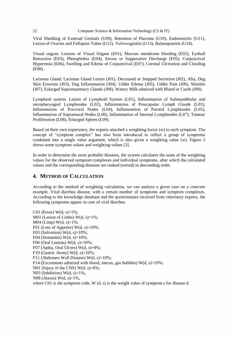
Based on their own experience, the experts attached a weighting factor (w) to each symptom. The
concept of “symptom complex” has also been introduced to reflect a group of symptoms
combined into a single value argument, which is also given a weighting value (w). Figure 3 shows some symptom values and weighting values [3].
In order to determine the most probable diseases, the system calculates the sums of the weighting
values for the observed symptom complexes and individual symptoms, after which the calculated values and the corresponding diseases are ranked (sorted) in descending order.
4. METHOD OF CALCULATION According to the method of weighting calculation, we can analyze a given case on a concrete
example. Viral diarrhea disease, with a certain number of symptoms and symptom complexes.
According to the knowledge database and the questionnaire received from veterinary experts, the
following symptoms appear in case of viral diarrhea:
C01 (Fever) W(d, s)=1%;
M01 (Lesion of Limbs) W(d, s)=1%; M04 (Limp) W(d, s)=1%;
F01 (Loss of Appetite) W(d, s)=10%;
F03 (Salivation) W(d, s)=10%; F04 (Stomatitis) W(d, s)=10%;
F06 (Oral Lesions) W(d, s)=10%;
F07 (Aphta, Oral Ulcers) W(d, s)=8%;
F10 (Gastric Atony) W(d, s)=10%; F11 (Abdomen Wall Disease) W(d, s)=10%;
F14 (Excrements admixed with blood, mucus, gas bubbles) W(d, s)=10%;
N01 (Injury of the CNS) W(d, s)=6%; N03 (Inhibition) W(d, s)=1%;
N08 (Ataxia) W(d, s)=1%,
where C01 is the symptom code, W (d, s) is the weight value of symptom s for disease d.

Computer Science & Information Technology (CS & IT) 23
Thus, it is possible to calculate the sum of weighting coefficients of symptoms by disease. A simple sum of weights of symptoms for the disease is calculated using a formula:
(1)
where d is the disease, So is the observed set of symptoms, W (d, s) is the weighting value of
symptom s for disease d.
For the above example with the disease "viral diarrhea», the values of the arguments will be
equal to:
With So = 14:
W(d, s0)= W (C01) + W (M01) + W(M04) + + W (F01) + W (F03) + W (F04) +W (F06) + W
(F07) + W (F010) + W+ +(F011) + W (F014) + W (N01) + W (N03) + +W (N08)=100%
Due to the fact that several symptom complexes k with different weights w can be defined for
disease d, the symptom complex with the highest weighting is taken into account, each symptom
of which includes the many symptoms observed:
(2)
i.e. for (3)
where: K (d) - symptom complexes of the disease d, S (k) is the set of symptoms of symptom
complex k, W (d, k) - weight coefficient of symptom complex k, for disease d.
Thus, for viral diarrhea, the symptom complex with the highest weighting factor is kmax, which
includes symptoms F01, F03, F04, F06, F07, i.e. S(kmax)=5.
In total for the disease "viral diarrhoea" the symptom complex kmax will give W (d, kmax) =65%,
according to the knowledge base provided by veterinary experts.
Taking into account the above mentioned number of symptoms not included in the symptom
complex will be calculated as Sx=S0-S(kmax) difference, i.e. for viral diarrhea Sx=9. Thus, it is
easy to calculate W(d, Sx)=52%.
The total sum of weights R for observed symptoms So and symptom complexes S(kmax) for
disease d is calculated by formula [12] :
(4)
For viral diarrhoea, the total sum of R weights for the observed symptom group Sy (F11, F14)
and symptom complexes S(kmax) at the same time will be Wr (d,S)=85%.
After calculating the total sums, the obtained data are sorted in descending order.
Thus, we can conclude that the introduction of such a parameter as a symptom complex leads to a
more accurate definition of this or that disease. The results obtained as a percentage may show
that the observed symptoms belong to a certain diagnosis [3].

24 Computer Science & Information Technology (CS & IT)
5. DATABASE, THEIR IMPLEMENTATION For the central database as well as for its local version, relational databases (MS SQL Server
2019 and SQLite) are used on the user device. Figure 4 presents the database structure in terms of
knowledge storage about diseases, symptoms and symptom complexes [3].
Figure 4: Database structure
Knowledge database contains information about 16 major infectious diseases and 103 symptoms of diseases. The database stores the subject area knowledge needed to solve problems, including
age, cow breed, symptoms, photographs, and other relevant information. The database is
developed on:
Figure 5: Veterinarian tablet web interface
- Operating system: Windows Server 2019 Standard;
- Web server: Internet Information Services; - DBMS: SQL Server 2017 Standard;
- Platform: NET 4.5.2, language C #;

Computer Science & Information Technology (CS & IT) 25
- Framework: DevExpress XAF 18.2 - a set of libraries to help the developed program with modern high-quality functionality [3].
6. EXPERT SYSTEM EVALUATION – TEST AND RESULTS
The evaluation process was carried out due to the user-friendliness of the user interface and system utilization efficiency testing. The reliability of the system diagnosis was evaluated with
the participation of two groups of senior veterinary students of KATU named after S. Seifullin.
Figure 6: Questionnaire of Veterinary Students
Table 1: Changes Characteristic in the Disease Diagnosis Using Tablet versus Diagnosis without Tablet
Job
Number
Name of the
disease
Characterization of changes in the diagnosis of the disease when using a
tablet, compared with diagnosis without a tablet
001 Anthrax A significant increase in the probability of diagnosing anthrax – from 20% to 69% (3.43 times)
002 Foot and mouth disease
The increase in the probability of diagnosis of foot and mouth disease - from 70% to 93% (1.33 times).
003 Tuberculosis A significant increase in the probability of diagnosis of tuberculosis - from
12% to 89% (7.41 times)
004 Brucellosis A slight decrease in the probability of diagnosis of brucellosis - from 82% to 81%
005 Rabies A slight decrease in the probability of a correct diagnosis of rabies is from 100% to 92%. Probably by providing subjects with additional options
006 Pasteurellosis An increase in the probability of correct diagnosis of pasteurellosis - from
44% to 54% (1.23 times)
007 Trichophytosis
A slight increase in the probability of a correct diagnosis from 68% to 74%
008 Leukemia A significant increase in the probability of a correct diagnosis of leukemia - from 10% to 86% (8.64 times)
009
Infectious
Rhinotracheitis
Decrease in probability of correct diagnosis of infectious rhinotracheitis - from 54% to 44%
010 Viral diarrhea A slight increase in the probability of a correct diagnosis of viral diarrhea - from 20% to 22%
011 Nodular dermatitis of cattle
Increasing the likelihood of a correct diagnosis of nodular cattle dermatitis - from 80% to 90% (1.13 times).
012 Emphysematous cattle carbuncle
An increase in the probability of a correct diagnosis of cattle emphysematous carbuncle - from 58% to 67% (1.15 times).
013 Salmonellosis Reducing the likelihood of a correct diagnosis of salmonellosis - from 40%

26 Computer Science & Information Technology (CS & IT)
In Figure 6: green indicates that this student has answered the question correctly, and at the end
of the table is information on the questions correctly answered and their proportion compared to the total number of tasks.
Figure 7: Diagram of Correct Answers Quality Representation
The second group of students worked with the “Veterinary Tablet”. This group worked on the
same test tasks as the first one. Figure 7 provides information on the quantity and quality of correct answers. After calculating and analysis of the data obtained, we concluded that the
percentage of correct answers using the “Veterinary Tablet” was 69%.
As the diagram in Figure 7 shows, most students answered the questions correctly. Colors show
the ratio of their answers (diagnosis) depending on the task number. The right column of the
diagram shows the colors that correspond to a certain diagnosis of the disease, for example,
brucellosis is indicated in orange, and etc.
We have analyzed the most common symptoms that students chose when answering questions
using the tablet, analyzed the number of selected symptoms and their types [3].
According to Figure 8, the most frequent symptoms as a result of the test were: fever, stomatitis,
salivation, lameness. The rest of the symptoms were less frequent.
After comparing all the data obtained, we came to the conclusion about the probability of making
the right diagnosis in cases with and without the application. This information is shown in Table
1.
Table 1 shows the changes characteristic in the disease diagnosis using tablet versus diagnosis
without Tablet. The analysis of changes in correct answers taking into account each symptom and set of symptoms is performed.
The average time to answer each question has also been calculated. This information is reflected
in Table 2.
to 35%.
014 Colibacillosis An increase in the probability of correct diagnosis of colibacillosis - from 38% to 58% (1.52 times)
015 Rotaviruses A significant increase in the probability of correct diagnosis of rotavirus infections - from 8% to 25% (3.13 times).
016 Coronaviruses The correct diagnosis when using the tablet was 25%, without using the tablet, no one was tested correctly

Computer Science & Information Technology (CS & IT) 27
According to Table 2, we can conclude that the average time to conduct diagnostics for known symptoms is 2-5 minutes. There are no dependencies between the quality of the diagnosis and the
time spent on the test task.
For diseases such as leukaemia, tuberculosis, anthrax, rotavirus infections, a clear improvement
in the correct diagnosis with help of the veterinary tablet was found (a total of 12 out of 16 test
questions showed an improvement in the quality of diseases diagnosis). Separately considering
rotavirus infections, the developed software allowed the correct diagnosis of diseases in a quarter of cases, given that without the veterinary tablet no test subjects in this case answered the
questions correctly.
Figure 8: Symptom Distribution Using “Veterinary Tablet”
Table 2: Characteristics of disease diagnosis time with the use of veterinary tablet
Time to make an erroneous
diagnosis (seconds)
Time to make the correct diagnosis
(seconds)
Row
names Min. Avg. Max. Min. Avg. Max.
001 72 255 938 82 213 375
002 - - - 62 125 284
003 181 181 181 65 113 201
004 123 301 478 61 165 540
005 - - - 64 163 771
006 95 185 700 61 142 294
007 111 201 338 62 148 539
008 89 137 185 64 162 622
009 86 246 937 94 255 584
010 71 207 456 78 160 346
011 83 110 136 60 132 276
012 111 157 205 62 244 1255
013 70 227 900 75 112 198
014 60 93 146 74 142 313
015 63 159 632 64 129 243
016 77 123 319 99 131 185
Total: 92 184 468 70 158 439
Summing up, we can conclude that the software implemented has improved, on average, the results of correct diagnosis from 42% to 69% [3].

28 Computer Science & Information Technology (CS & IT)
In the process, some shortcomings of the selected software testing method were revealed. Firstly,
it is the impossibility of veterinarians to work directly with the studied animal directly, as well as
the limited initial data on disease symptoms and the lack of visibility of the whole picture in general.
7. DEVELOPMENT OF AN ALGORITHM FOR PROCESSING DIGITAL DATA
FOR MONITORING THE PRODUCTIVITY OF FARM ANIMALS WITH
ELEMENTS OF MACHINE LEARNING
One of the main tasks of the work is the development of software for predicting the productivity of farm animals using data from the smaXtec bolus system and data on milk production of
animals. The smaXtec system allows real-time reception of such indicators as: pH, body
temperature of the animal, measurement of movement activity, etc. The bolus is injected into the
rumen of the animal, and then enters the ruminant stomach, the reticulum, and transfers the data from there. An orally administered bolus measures temperature and activity (via an
accelerometer), continuously at 10-minute intervals, while the activity measurement is
independent of rumen mobility. Typical increases in activity during sexual activity are detected immediately and trigger notifications. The individual activity levels of the cow are taken into
account when processing the data. Fever events are presented to the farmer as a graph or list in
the cow's profile and in the fertility section of the dashboard. In this way, the history of
previously successful inseminations of dairy cows can be documented in the software for calculating the expected lactation. We used the data of the cattle herd LP "Mambetov and K",
consisting of 800 heads of the “simmental” population in the period from 2019 to 2020. (for
about 30 thousand data points for all animals).
Figure 9: Architecture of the smaXtec system. The smaXtec solution consists of a reticuluminal bolus (1),
an online data platform (2), infrastructure including readers and climate sensors (3).

Computer Science & Information Technology (CS & IT) 29
Table 3: Data for each animal
In accordance with the tasks set, such indicators were selected: 1. Body temperature of the animal;
2. Normal body temperature of the animal;
3. Activity index; 4. Body temperature without drinking cycle;
5. Milk yield;
Thus, a library in the Python programming language was developed to extract data from the smaXtec system. The library retrieves data by using REST API technology.
Based on the data obtained and the purpose of the work (forecasting milk production), the most suitable methods are: "Learning with a teacher", exactly regression methods and forecasting
methods.
According to the graph of the distribution of milk production by day (Figure 10), you can see
useful data.
Animal ID Date
Body
temperatu
re (° C)
Normal
body
temperatur
e (° C)
Index of
the activity
Body
temperatur
e without
water
consumpti
on (° C)
Milk
yield
(kg))
DE0667033081 18.10.2019 39.19 40.000000 13.223118 39.826875 6.35
DE0667033081 18.10.2019 39.19 40.000000 13.223118 39.826875 10.34
DE0667033081 19.10.2019 39.34 40.000000 14.251181 39.871319 6.45
DE0667033081 19.10.2019 39.34 40.000000 14.251181 39.871319 0.00
DE0667033081 19.10.2019 39.34 40.000000 14.251181 39.871319 10.49
... ... ... ... ... ... ...
DE0953378924 21.12.2020 38.69 40.000000 10.522472 39.016806 0.00
DE0953378924 21.12.2020 38.690951 40.000000 10.522472 39.016806 4.99
DE0953378924 23.12.2020 38.826500 40.000000 14.486500 39.186528 5.14
DE0953378924 23.12.2020 38.826500 40.000000 14.486500 39.186528 0.00
DE0953378924 23.12.2020 38.826500 40.000000 14.486500 39.186528 4.77

30 Computer Science & Information Technology (CS & IT)
Figure 10: Distribution of milk yield sorted by days.
The stage of applying machine learning methods follows after the initial analysis and data preprocessing. Based on the data, the most suitable machine learning method is polynomial
regression.
Figure 3 is a block diagram of the overall software architecture.
The software architecture consists of 3 main components:
1) System for remote monitoring of the condition of animals smaXtec; 2) Computing part (machine learning);
3) Interface for the farmer;
Figure 11: General architecture of the software.
A simple and straightforward architecture makes it faster to make any changes, as well as easier
to integrate with other systems.

Computer Science & Information Technology (CS & IT) 31
Figure 12: Correlation matrix of the obtained data.
As a result of visualization of the correlation matrix in the form of a heat map, presented in
Figure 12, we concluded that there is no statistical relationship between such parameters as: body temperature, normal body temperature, body temperature without a drinking cycle, movement
index. In this case, changes in the values of one or more of the above values do not accompany a
systematic change in other values.
Figure 13: Regression analysis of the obtained data.
As a result of the conclusions made, we came to the need to use a simple linear regression for
possible dependencies of the parameters of the initial data and the need to predict the volume of
milk yield. In Figure 13, we see that the resulting errors do not have a normal distribution and the data variations around the regression line are not constant. Thus, prediction of the milk
production of animals based on the above parameters (body temperature, normal body
temperature, body temperature without a drinking cycle, movement index, milk yield) is also impossible.
Thus, we can conclude that the initial data (body temperature, normal body temperature, body
temperature without a drinking cycle, movement index, milk yield) obtained from the smaXtec

32 Computer Science & Information Technology (CS & IT)
bolus system and data on the milk production of animals are not dependent. As a result, there is no need to use the initial data parameters for the effect on the volume of milk yield.
8. CONCLUSIONS
Upon analyzing the problem of cow diseases diagnostics, we came to the conclusion that it is necessary to develop an expert system of cattle diseases diagnostics. When setting the main tasks
to build an expert system, the main one was to determine the input and output data of this system.
By using the induction method, we have identified separate groups of input and output data, which will be used to build this system. The next stage was the creation of a generalized web
architecture, with the indication of individual functional blocks and equally developed the basic
scenario of the use of the intellectual system. When diagnosing a disease, the way the knowledge base is presented plays an important role, which in turn depends on the experience of team of
veterinarians. Information on main symptoms and diseases has been collected through
questionnaires and this information is structured and presented for better understanding. Thus, a
model of knowledge representation has been developed, which leads to an accurate diagnosis. Together with a team of veterinarians, each symptom and symptom complex was given the
weight coefficients required for a more accurate diagnosis of the disease.
Thus, we can conclude that the developed expert system for addressing veterinary medicine
challenges is effective. By comparing the percentage ratios of the results of the questionnaire of
two groups, it becomes obvious that its use is expedient. A detailed analysis of the test subjects' answers has been made and all regularities in both cases of testing have been taken into account.
Conclusions were made that the process of diagnosing diseases is simplified in terms of speed of
decision-making and their reliability, a direct correlation between the number of detected initial
symptoms of the disease and the correct formulation of the diagnosis was revealed. Also, with the participation of veterinary students, an evaluation of the user interface was conducted, which
included checking system design and correct compilation of the knowledge base to meet user
requirements.
In summary, the developed software has shown its need for use. In future, the database of expert
system on diseases and symptoms will be expanded, all deficiencies related to the convenience of
the user interface and the operation of the program in general will be taken into account and eliminated.
An expert system under development provides information on 16 major infectious diseases and 103 symptoms, which is currently being developed and populated in the database. The
development works are carried out in the S. Seifullin Kazakh Agro Technical University, at the
faculties of computer systems and veterinary medicine.
In the future, work will also be done to integrate the system under development with existing
animal control systems, to automate the processes of their interaction and data exchange. It is
necessary to work with symptoms and weight values, that is, it is necessary to work on choosing an index of the significance of the manifestation of a symptom, instead of its usual manifestation
or absence.
ACKNOWLEDGEMENTS
The authors would like to thanks for the veterinarian team expertise, Faculty of Veterinary Science, Kazakh Agro Technical University named after S. Seifullin. The work was carried out as

Computer Science & Information Technology (CS & IT) 33
part of the project “Transfer and adaptation of innovative technologies to optimize production processes at dairy farms in Northern Kazakhstan” (BR06349515).
REFERENCES
[1] E. Tullo, I. Fontana, D. Gottardo, K.H. Sloth, M. Guarino. Technical note: Validation of a
commercial system for the continuous and automated monitoring of dairy cow activity// J.Dairy Sci.
99:7489–7494. http://dx.doi.org/10.3168/jds.2016-11014. American Dairy Science Association,
2016.
[2] Emre Aydemir, İnci Bilge. Automation Applications in Integrated Animal Production System.
Turkish Journal of Agriculture - Food Science and Technology, 8(3): 643-644, 2020. DOI:
https://doi.org/10.24925/turjaf.v8i3.643-644.3133.
[3] O. Shopagulov, I. Tretiakov, A. Ismailova, “An expert system for diagnosis cow diseases,” Journal of
Theoretical and Applied Information Technology, No 15, Vol.98., 2020, pp. 3106-3115.
[4] Ermekov Aidar. Meat March, 2013, [Online]. Available at: http://mk-kz.kz/article/2013/02/11/810619-myasnoy-marsh.html/ (in Russian).
[5] Committee on Statistics of the Ministry of National Economy of the Republic of Kazakhstan:
[Online]. Available at: http://www.kazagro.kz/analiticeskij-obzor-po-zivotnovodstvu/ (in Russian).
[6] The Committee on Statistics of the Ministry of National Economy of the Republic of Kazakhstan:
[Online]. Available at: https://www.zakon.kz/4951625-obem-veterinarnyh-uslug-v-kazahstane.html/
(in Russian).
[7] L. I. Zubkova, “The effect of diseases of the udder on the milk productivity of cows,” Dairy and beef
cattle breeding, vol. 4, 2005, pp. 35-37. (in Russian).
[8] H. Qin, J. Xiao, X. Gao, H. Wang, “Horse-Expert: An aided expert system for diagnosing horse
diseases,” Veterinary Sciences, vol. 4, 2016, pp. 907-9015.
[9] M. Dorosh, Diseases of cattle, Veche, Moscow, 2007, 7 p. (in Russian).
[10] Yu. N. Kozlov, N. M. Kostomakhin, Genetics and selection of farm animals, Kolos, Moscow, 2013, 100 p. (in Russian).
[11] O. V. Zavyazkin, Breeding and keeping cattle, BAO, Kiev, 2012, 100p. (in Russian).
[12] Fu Zetian, Xu Feng, Zhou Yun, Zhang Xiao Shuan, “Pig-vet: a web-based expert system for pig
disease diagnosis,” Expert Systems with Applications, vol. 29, pp. 93-103, 2005.
[13] Daoliang Li, Zetian Fu, Yanqing Duan, “Fish-Expert: a web-based expert system for fish disease
diagnosis,” Expert Systems with Applications, vol. 23, pp. 311-320, 2002.
[14] Paolo Liberati, Paolo Zappavigza, “Improving the automated monitoring of dairy cows by integrating
various data acquisition systems,” Computers and electronics in agriculture, vol. 68, pp. 62-67, 2009.
[15] D. Rice, Common dog diseases and health problems 4-H Companion Animal Health, 2014, [Online].
Available at: https://www.extension.purdue.edu/extmedia/4H/4-H-852-W.pdf/
[16] E. B. Hunt, Artificial Intelligence, New York, San Francisco, London, Academic Press, 558 p, 1975. [17] M. I. Makarov, V. M. Lokhin, Intelligent Automatic Control System, Moscow: Fizmatlit, 2001, 576
p. (in Russian).
[18] T. A. Gavrilova, V. F. Khoroshevsky, Knowledge Base of Intelligent Systems, St. Petersburg: Piter,
2000, 384 p. (in Russian).
[19] D. Zeldis and S. Prescott, “Fish disease diagnosis program – Problems and some solutions”
Aquacultural Engineering, vol. 23, no. 1–3, 2000, pp. 3-11.

34 Computer Science & Information Technology (CS & IT)
AUTHORS
Shopagulov Olzhas Almatovich, Doctoral student, Department of Information
Systems, Kazakh Agro Technical University named after S.Seifullin, Nur-Sultan,
Kazakhstan. In 2014 he graduated the Eurasian National University named after L.N.
Gumilyov, received a bachelor's degree in radio engineering, electronics, telecommunications. Also in 2017, he graduated from S. Seifulin Agro Technical
University with a radio engineering, electronics, telecommunications master’s
degree. He is project assistant on the development of an expert system for solving the
problems of veterinary medicine (on the example of a dairy farm in Northern
Kazakhstan). His research interests include the development of information systems, researches related to
big data, as well as works related to data transfer.
Tretyakov Igor Igorevich recieved bachelor in technics and technologies from the
Eurasian National University, Astana, Kazakhstan, in 2009. From 2009 to 2012, he
was a software developer of various state information systems for electronic
government. From 2012 to 2016 he was a software developer, data analyst and project manager for project in animal husbandry, animal recording in Kazakhstan. Participated
in projects for animal genomic (gBLUP) and index evaluation in collaboration with
INRA - French National Institute for Agricultural Research (dairy cattle) and
Agricultural Business Research Institute, Australia (beef cattle). Since 2018, he is a
lead of IT group in S.Seifullin Kazakh Agro Technical University in the "Transfer and
adaptation of innovative technologies to optimize production processes at dairy farms in Northern
Kazakhstan" project. His interests include software development for web and mobile, automation systems
and data analytics in agriculture.
Ismailova Aisulu Abzhapparovna, Doctor of Philosophy (PhD), Senior Lecturer.
Received the bachelor degree in Physics and Mathematics from the Korkyt Ata Kyzylorda Pedagogical Institute, in 1993. Received the master’s degree in Information
Technology from the Eurasian National University named after L. N. Gumilyov, in
2006. From 2011 to 2014, she graduated a doctoral program at the Faculty of
Information Technology at the Eurasian National University named after L.N.
Gumilyov. His research interests are 3D modeling, working with spatial data,
development of methods and software for creating information systems.
© 2021 By AIRCC Publishing Corporation. This article is published under the Creative Commons
Attribution (CC BY) license.

David C. Wyld et al. (Eds): SEAS, CMCA - 2021
pp. 35-52, 2021. CS & IT - CSCP 2021 DOI: 10.5121/csit.2021.110203
LOSSLESS STEGANOGRAPHY ON
ORTHOGONAL VECTOR FOR 3D H.264 WITH LIMITED DISTORTION DIFFUSION
Juan Zhao1 and Zhitang Li2
1School of Mathematics &Computer Science,
Wuhan Polytechnic University, Wuhan 430048, China 2Institute of Computer Science and Technology, Huazhong University
of Science and Technology, Wuhan 430074, China
ABSTRACT
In order to improve the undetectability, a lossless algorithm based on orthogonal vectors with
limited distortion diffusion for 3D H.264 video is proposed in this paper. Inter-view distortion
drift is avoided by embedding data into frames, which do not predict other views. Three
conditions and pairs of coefficients are proposed to prevent intra-frame distortion diffusion.
Several quantized discrete cosine transform coefficients are chosen from an embeddable
luminance 4×4 block to construct a carrier vector, which is modified by an offset vector. When
the carrier vector and the offset vector are orthogonal or near to be orthogonal, a data bit can be
hidden. Experimental results indicate that the method is effective by enhancing peak signal-to-noise ratio with 7.5dB and reducing the Kullback-Leibler divergence with 0.07 at least.
More than 1.7×10¹⁵ ways could be utilized for constructing the vectors, so it is more difficult for
others to steal data.
KEYWORDS
Lossless Steganography, Reversible Data Hiding, Orthogonal Vector, 3D H.264, Distortion Drift
1. INTRODUCTION
The most significant requisite of steganography, which can be used to hide secret message into
innocuous-looking media, is imperceptibility in covert communication. However, the host media will be distorted permanently if general steganography algorithms are used to hide information.
Permanent damage is unbearable to medical images, military, law enforcement [1] and other
sensitive fields. Therefore, lossless steganography (a kind of reversible data hiding)[2], videlicet reversible steganography or distortion-free steganography, which can restore the impaired video
after extracting the secret information, has been a hot topic. Besides the sensitive fields, lossless
steganography methods can also be employed in error concealment and other fields.
Histogram shifting (HS) [3-10] and difference expansion (DE) [11-15] are two principal lossless
steganography approaches. In addition, integer pair swap (IPS) [16], pair-wise logical computation
[17], and some other methods [18][19] have been employed to hide information reversibly. In typical HS algorithm [3], information is hidden into the peak points of a medium histogram. The
number of embeddable data bits depends on the pixel number of the peak point in the histogram.
The hierarchical relationships of original images are used, and the difference values between pixels are altered to hide data in [5]. All pixels are classified into wall pixels and non-wall pixels in [4],

36 Computer Science & Information Technology (CS & IT)
where interpolation and direction order are used for hiding data. In [6], the closest adjacent pixels are used to predict the visited pixel value and evaluate its just noticeable difference.
Prediction-error shift is used to improve the embedding performance in [8, 9]. In [9], multiple pairs
of expansion bins are utilized for each histogram , and the multiple-expansion-bin-selection for
optimal embedding is formulated as an optimization problem.
In difference expansion method [11], the difference between two neighboring pixels is doubled to
hide message. The secret information and a compressed location map are hidden into the difference values. To increase the payload, 16 bits are embedded into a 4×4 pixel block in a two-dimensional
DE scheme [12].The host image is divided into non-overlapped equal-sized blocks in the
high-fidelity technique [13] based on prediction-error expansion and pixel-value-ordering. Bidirectional difference expansion is used in [14] with three steps.
However, in traditional steganography algorithms, the selection space of embeddable location is
small. How to improve the undetectability and security of lossless steganography algorithm is a key issue of covert communication. Video has so many frames that it can ensure adequate storage
space. [20] Hence, through embedding a little information into a frame, we can guarantee video
quality and improve the invisibility and undetectability. H.264 is the standard for video compression with high compression efficiency. 3D H.264 video is encoded or decoded through
multi-view coding, which is an extension of H.264. At the encoder, intra-frame, inter-frame and
inter-view predictions are used to compress the original YUV videos into a 3D H.264 video. In order to watch the video on the screen, the 3D H.264 video needs to be decompressed into YUV
videos by intra-frame, inter-frame and inter-view predictions at the decoder. So if one block of a
video is changed to embed data, the other blocks of the same frame, other frames or views in the
corresponding YUV videos may also be modified, it is called intra-frame, inter-frame, or inter-view distortion drift [21], which is not considered in the literatures on 3D video data hiding
[22-24].
In order to improve the undetectability and security of steganography, we present a novel lossless
steganography algorithm based on orthogonal vector (If the inner product of two vectors is zero, it
is called that the two vectors are orthogonal) for 3D H.264 video with limited distortion drift in this
paper. Inter-view distortion propagation is avoided by embedding information into frames that do not predict other views. Embeddable blocks based on restrictive conditions are selected to prohibit
intra-frame distortion shift. A carrier vector is composed of some quantized discrete cosine
transform (QDCT) coefficients or coupling coefficients in one embeddable 4×4 block. An offset vector is set for recording the modification of the carrier vector. By dividing the inner product of
the carrier vector and offset vector into several disjoint intervals, the information is hidden
according to the interval of inner product. The carrier vector is not altered for hiding information 0; otherwise, the offset vector is added to or subtracted from the carrier vector according to the inner
product of the two vectors. The receiver extracts information and restores the carrier according to
the interval of inner product.
Compared with the current methods, the contributions of this paper are presented as follows. A.
Three conditions and two sets of coupling coefficients are proposed for limiting intra-frame
distortion drift. B. When the three conditions are used to avoid intra-frame distortion drift, over
1.7×10¹⁵ ways of constructing the carrier vector and its offset vector increase the difficulty for
others stealing data.
The rest of the paper is organized as follows. The way of avoiding distortion diffusion for 3D H.264 video is brought in Section 2. Section 3 describes the lossless steganography algorithm and
Section 4 gives the experimental results. At last, the paper is concluded in Section 5.

Computer Science & Information Technology (CS & IT) 37
2. DISTORTION DIFFUSION PREVENTION The original block denoted by BO in the original YUV video is processed by equation (1) at the 3D
H.264 encoder.
BO - BP = BRO (1)
Where BP is the prediction block and BRO is the residual block. Undergoing discrete cosine
transformation and quantization, the residual block BRO becomes a QDCT block (denoted by Y). Finally, YUV videos will be changed into 3D H.264 video by entropy encoding of QDCT blocks.
Because this entropy encoding is a lossless compression process, at the decoder, the data embedded
in some QDCT coefficients could be extracted completely after entropy decoding (lossless
decompression). Undergoing the inverse quantization and inverse discrete cosine transform, the QDCT block Y becomes a residual block denoted by BR (Cause discrete cosine transformation and
quantization are loss compressions, BR is different from the original residual block BRO), which will
be added to the prediction block BP for reconstructing the video.
The prediction block BP of a block in a frame could be computed through inter-view prediction,
inter-frame prediction, or intra-frame prediction. Horizontal inter-frame prediction and vertical inter-view prediction of a 3D H.264 video with hierarchical B coding and two views are illustrated
in Figure 1[7]. There are 16 frames in one group of picture, where each view has eight frames. Only
intra-frame prediction is used for I0 frame, so the distortion of other frames will not affect I0 frame.
However, hiding data into I0 frame will sway all the frames in the two adjacent groups of pictures predicted by I0 frame. By contrast, embedding data into P0 frame will not lead to inter-view
distortion drift because P0 frame in the right view does not predict frames in the left view.
Furthermore, inter-view distortion drift and inter-frame distortion drift could be avoided by embedding data into b4 frames. Therefore, compared with embedding data into I0 frames, better
video quality can be achieved through embedding data into P0 or b4 frames. However, b4 frame is
located at the lowest level and is easy to be discarded during the process of transmission in the network. Compared with b4 frame, better video quality cannot be acquired through embedding data
into P0 frame. However, P0 frame is a key picture at the highest level, resulting that it cannot be lost
easily during the process of the network transmission. Consequently, stronger robustness can be
obtained by hiding data into P0 frame compared with b4 frame. Therefore, the best combination of video quality and robustness can be obtained by hiding data into P0 frame, so it is selected to embed
information in this paper.
Time
Views
Left View
Right View
I0 B3 B2
b4
B1B3 B3 B2 B3
P0 B3 b4 b4 b4B2 B3
I0
P0
T0 T7T5 T6T4T3T2T1 T8
Figure 1. Prediction structure of3D H.264 with two views
At the encoder, through using inter-view prediction, inter-frame prediction, or intra-frame
prediction, the prediction block BP of a block is achieved to compute its residual block BRO,
which will be changed into a QDCT block Y by the 4×4 discrete cosine transform and
quantization formulated as

38 Computer Science & Information Technology (CS & IT)
00 01 02 03
10 11 12 13
20 21 22 23
30 31 32 33
( ) ( / ) ,RO T
f f f
Y Y Y Y
Y Y Y YY round C B C E Q
Y Y Y Y
Y Y Y Y
(2)
where Q is the quantization step size, ⨂is a math operator, by which each element in the
former matrix is multiplied by the value at the corresponding position in the latter matrix,
2 2
2 2
2 2
2 2
/ 2 / 2
/ 2 / 4 / 2 / 4
/ 2 / 2
1 1 1 1
2 1 1 2,
/ 2 / 4 / 2 /
1 1 1 1
1 2 1 42
1/ 2, 2 / 5.,ff
a ab a ab
ab b ab bE
a ab a ab
a a
C
b b b b
a b
When a data bit is hidden into one QDCT block Y by modifying some QDCT coefficients, the
QDCT block after embedding data is denoted by YEmb. Let ∆Y denote the modification caused
by hiding information, it can be computed as
∆Y = YEmb - Y. (3)
At the decoder, the residual block acquired by inverse quantization and 4×4 inverse discrete cosine
transform is denoted by BR , which can be calculated by
,R T
d d dB round C Y E C (4)
where
2 2
2 2
2 2
2 2
1 1 1 1
1 1 / 2 1 / 2 1, .
1 1 1 1
1 / 2 1 1 1 / 2
d d
a ab a ab
ab b ab bC E
a ab a ab
ab b ab b
When a data bit is embedded through modifying some QDCT coefficients of one block, the
residual block after embedding data is denoted by BREmb. Let ∆BR depress the variation of the residual block between before and after hiding information. It can be computed as
( ) .R REmb R T
d d dB B B round C Y Q E C (5)
Take the QDCT coefficient Y32 as an example to explain the distortion caused by hiding data.
Suppose r is added to Y32, the modification of the QDCT block for hiding data is
0 0 0 0
0 0 0 0
0 0 0 0
0 0 0
Y
r
,
then the alteration of the corresponding block in YUV video is
1 1 1 1
2 2 2 21.
2 2 2 22
1 1 1 1
RQabrB
(6)

Computer Science & Information Technology (CS & IT) 39
Similarly, changing any one other QDCT coefficient in a 4×4 block will cause the variation of
the whole block in the corresponding YUV video. In the same way, for an 8×8 block,
modifying one QDCT coefficient will alter the whole 8×8 block, whose affected region is
bigger than that of the 4×4 block. In addition, only two kinds of transformations, 4×4 transformation and 8×8 transformation, are used in 3D H.264 standard. Hence, the 4×4
transform block is selected to embed information in this paper.
It can be inferred that the edge pixels denoted by c0…c12 (shown in Figure 2) may be changed
by hiding data into some QDCT coefficients of the blocks Bi,j-1 (the position of a block is
expressed by I and j), Bi-1,j-1, Bi-1,j, and Bi-1,j+1. On one hand, when inter-view prediction or inter-frame prediction is employed to compute the prediction block denoted by BP
i,j, the block
Bi,j will not be affected by the change of c0 …c12, because BPi,j is calculated by referring other
frames. On the other hand, when intra-frame prediction is used by the current block Bi,j, its
prediction block BPi,j will be reckoned by the pixels c0 …c12. Therefore, the hiding induced
deviation of the blocks Bi,j-1, Bi-1,j-1, Bi-1,j, and Bi-1,j+1 will propagate to the block Bi,j. This is
called as intra-frame distortion drift. However, according to the intra-frame prediction modes
shown in Figure 2, it can be seen that the block Bi,j is not affected by the thirteen pixels c0 …c12 at the same time. For instance, when intra-frame prediction mode 0 is used by the current block
Bi,j, only pixels c1, c2, c3, andc4 are used to predict the block Bi,j, so the distortion of the blocks
Bi,j-1, Bi-1,j-1, and Bi-1,j+1 will not drift to the block Bi,j. Similarly, we can conceive the influence of Bi,j over Bi,j+1, Bi+1,j+1, Bi+1,j, and Bi+1,j-1. Therefore, some conditions could be used to prevent
intra-frame distortion drift.
Bi-1,j-1 Bi-1,j Bi-1,j+1
Bi,j-1 Bi,j Bi,j+1
Bi+1,j+1Bi+1,jBi+1,j-1
1c
0 5
4
6
1
8
73 0
1
3
0c
12c11c10c9c
8c7c6c5c4c3c2c3
V
F
(a) (b) (c)
Figure 2. Intra-frame prediction mode (a) block position (b) the predictive direction of 4×4 and 8×8 luma
block.(c) the predictive direction of 16×16 luma block.( In mode 2, all elements are predicted with the average
of upper pixels denoted by F and left pixels denoted by V, i.e. Mean (F+V))
The prediction mode of intra-frame is denoted by prediction Mode. The mode type of macro block (MB) is denoted by mb_type. Let p be the mb_type of inter-view or inter-frame
prediction. If the mb_type of the block Bi,j+1 is p, the prediction block BPi,j+1 is calculated by
referring another frame, so the current block Bi,j will not predict the block Bi,j+1. Otherwise, when the intra-frame prediction modes 0, 3, 7 indicated in Figure 2(b), or 0 in Figure 2 (c) are
used by the block Bi,j+1, it can be seen from the predictive directions that the block Bi,j+1 will not
be predicted by the current block Bi,j. Therefore, if information is embedded into the QDCT coefficients of the current block Bi,j, whose right adjacent block Bi,j+1 meets Condition 1, the
evoked distortion will not drift to its adjacent block Bi,j+1.
Condition 1. , 1 , 1 (4 4 or 8 16 168) ( )
0,3,7_ 0i j i jB Bmb type p predictionMode
If the mb_type of the block Bi+1,j is p, the prediction block BPi+1,j is not calculated by referring
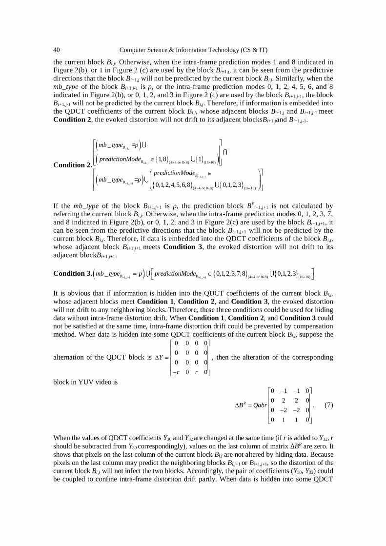
40 Computer Science & Information Technology (CS & IT)
the current block Bi,j. Otherwise, when the intra-frame prediction modes 1 and 8 indicated in Figure 2(b), or 1 in Figure 2 (c) are used by the block Bi+1,j, it can be seen from the predictive
directions that the block Bi+1,j will not be predicted by the current block Bi,j. Similarly, when the
mb_type of the block Bi+1,j-1 is p, or the intra-frame prediction modes 0, 1, 2, 4, 5, 6, and 8
indicated in Figure 2(b), or 0, 1, 2, and 3 in Figure 2 (c) are used by the block Bi+1,j-1, the block Bi+1,j-1 will not be predicted by the current block Bi,j. Therefore, if information is embedded into
the QDCT coefficients of the current block Bi,j, whose adjacent blocks Bi+1,j and Bi+1,j-1 meet
Condition 2, the evoked distortion will not drift to its adjacent blocksBi+1,jand Bi+1,j-1.
Condition 2.
1,
1,
1, 1
1, 1
4 4 or 8 8 16 16
4 4 or 8 8 16
( ) ( )
( ( 16) )
_
1,8 1
_0,1,2,4,5,6,8 0,1,2,3
i j
i j
i j
i j
B
B
B
B
mb type p
predictionMode
predictionModemb type p
=
=
If the mb_type of the block Bi+1,j+1 is p, the prediction block BPi+1,j+1 is not calculated by
referring the current block Bi,j. Otherwise, when the intra-frame prediction modes 0, 1, 2, 3, 7,
and 8 indicated in Figure 2(b), or 0, 1, 2, and 3 in Figure 2(c) are used by the block Bi+1,j+1, it
can be seen from the predictive directions that the block Bi+1,j+1 will not be predicted by the current block Bi,j. Therefore, if data is embedded into the QDCT coefficients of the block Bi,j,
whose adjacent block Bi+1,j+1 meets Condition 3, the evoked distortion will not drift to its
adjacent blockBi+1,j+1.
Condition 3. 1, 1 1, 1 (4 4 or 8 8) ( )16 16
_ 0,1,2,3,7,8 0,1,2,3i j i jB BpredictionModemb type p
It is obvious that if information is hidden into the QDCT coefficients of the current block Bi,j,
whose adjacent blocks meet Condition 1, Condition 2, and Condition 3, the evoked distortion
will not drift to any neighboring blocks. Therefore, these three conditions could be used for hiding
data without intra-frame distortion drift. When Condition 1, Condition 2, and Condition 3 could not be satisfied at the same time, intra-frame distortion drift could be prevented by compensation
method. When data is hidden into some QDCT coefficients of the current block Bi,j, suppose the
alternation of the QDCT block is
0 0 0 0
0 0 0 0
0 0 0 0
0 0
Y
r r
, then the alteration of the corresponding
block in YUV video is
0 1 1 0
0 2 2 0.
0 2 2 0
0 1 1 0
RB Qabr
(7)
When the values of QDCT coefficients Y30 and Y32 are changed at the same time (if r is added to Y32, r
should be subtracted from Y30 correspondingly), values on the last column of matrix ∆BR are zero. It
shows that pixels on the last column of the current block Bi,j are not altered by hiding data. Because
pixels on the last column may predict the neighboring blocks Bi,j+1 or Bi+1,j+1, so the distortion of the current block Bi,j will not infect the two blocks. Accordingly, the pair of coefficients (Y30, Y32) could
be coupled to confine intra-frame distortion drift partly. When data is hidden into some QDCT

Computer Science & Information Technology (CS & IT) 41
coefficients of the current block Bi,j, assume the alternation of the QDCT block is0 0 0 0
0 0 0
0 0 0 0
0 0 0 2
rY
r
,
then the alteration of the corresponding block in YUV video is
2
0 0 0 0
1 2 2 15.
1 2 2 14
0 0 0 0
R QB b r
(8)
When the values of QDCT coefficients Y13 and Y33 are changed at the same time (if r is added to Y13,
2r should be subtracted from Y33 correspondingly), the values on the bottom row of matrix ∆BR are
zero. It shows that pixels on the bottom row of the current block Bi,j are not changed by hiding data.
Because pixels on the last column may predict the neighboring blocks Bi+1,j,Bi+1,j-1orBi+1,j+1, so the distortion of the current block Bi,j will not infect the three blocks. Accordingly, the pair of
coefficients (Y13, 2Y33) could be coupled to prevent intra-frame distortion drift partly. Similarly, we
can get two sets of coupling coefficients, which are denoted by Cset and Rset.
00 02 10 12 20 22 30 32 01 03 11 13 21 23 31 33
00 20 01 21 02 22 03 23 10 30 11 31 12 32 13 33
{( , ), ( , ), ( , ), ( , ), ( , 2 ), ( , 2 ), ( , 2 ), ( , 2 )}
{( , ), ( , ), ( , ), ( , ), ( , 2 ), ( , 2 ), ( , 2 ), ( , 2 )}
set
set
C Y Y Y Y Y Y Y Y Y Y Y Y Y Y Y Y
R Y Y Y Y Y Y Y Y Y Y Y Y Y Y Y Y
=
=
When data is hidden into any coupling coefficients in Cset (if r is added to the former coefficient, r or
2r should be subtracted from the latter coefficient correspondingly), the values on the rightmost
column of matrix ∆BR are 0, so the distortion of the block Bi,j will not propagate its neighboring
blocks Bi,j+1 and Bi+1,j+1. Hiding data into any coupling coefficients in Rset, we can make the values at
the bottom row of matrix ∆BR be zero, so the distortion of block Bi,j will not affect its adjacent blocks
Bi+1,j,Bi+1,j-1, and Bi+1,j+1. It can be seen that the coupling coefficients in Rset could be combined with Condition 1 to avoid intra-frame distortion drift, and the coupling coefficients in Cset can be
combined with Condition 2 to eliminate intra-frame distortion drift. For instance, when the
adjacent blocks of the block Bi,j do not satisfy Condition 1 to 3 at the same time, if Condition 1 is satisfied by the adjacent block B i,j+1, it will not be affected by the block Bi,j. In addition, if coupling
coefficients such as (Y02, Y22) of Rset are selected from the block Bi,j for hiding data, the distortion of
the block Bi,j will not drift to its neighboring blocks Bi+1,j, Bi+1,j-1, and Bi+1,j+1.
3. LOSSLESS ALGORITHM BASED ON ORTHOGONAL VECTOR
The presented lossless steganography algorithm based on orthogonal vector for 3D H.264 video is
depicted in Figure 3. At first, the information to be hidden is encrypted, and the 3D H.264 video is entropy decoded to gain the QDCT coefficients and intra-frame prediction modes.
3.1. Information Embedding
Denote the threshold as H. We select a 4×4 luminance QDCT block of P0 frame in the right view
according to |Y00|≥H (threshold H=0,1,2,…. The bigger the threshold H is, the fewer embeddable blocks will be found, and the less the distortion will be. Compared with a block with small |Y00|, the
distortion caused by hiding data into a block with big |Y00| is less. ). If Conditions 1 to 3 are satisfied
at the same time, the current block is chosen as an embeddable block. In the 4×4 block, a QDCT
coefficient could be changed for hiding data, whereas only 16 selections can be used. If the third party identifies the marked block and the steganography algorithm, the probability for calculating
the hidden data bit directly is 1/16 =0.0625. In order to reduce the probability of being cracked, we

42 Computer Science & Information Technology (CS & IT)
embed data by choosing n QDCT coefficients from the block to make up a carrier vector denoted
by ψ =(x1,x2,…,xi,…,xn)(n∈[2,16]) such as ψ = (Y22,Y32) = (2, 0). Denote the carrier vector after
hiding data as 1 2( , ,..., ,..., )i nx x x x . In order to express the size of the modified value on carrier
vector for embedding data reversibly, we construct a non zero offset vector denoted
as∂=(z1,z2,…,zi,…,zn) such as ∂ = (0,1). Let φ be the included angle from the carrier vector ψ to the
offset vector ∂, and be the included angle from to ∂. Denote the length of the carrier vector
as |ψ|= 2 2 2 1/2
1 2( ... )nx x x . If the length |ψ| or the included angle φ is changed for hiding data, more
computations need to be done since the modification of QDCT coefficient must be computed. So
we hide data by changing the direction of the carrier vector, as shown in Figure 4 and (9), where the
value of QDCT coefficient is changed directly and simply.
Original 3D
H.264 videos
Select
embeddable block
Embed
information
+ +
Entropy
encode
Marked 3D
H.264 video
Select coefficients and
form carrier vector
Entropy
decode
(a)
(b)
Read
predictionMode
Read
mb_type
Set offset
vector
Encrypt
information
Select
embeddable block
+ +
Select coefficients and
form carrier vector
Entropy
decode
Read
predictionMode
Read
mb_type
Set offset
vector
Decrypt
information
Extract information
and restore video
Recovered 3D
H.264 video
Marked 3D
H.264 video
Entropy
encode
Figure 3. The flowchart of presented algorithm. (a) Embedding. (b) Extraction
0
'
0
2 2
'
(a) 0 (b) 0
Figure 4. The modification of carrier vector
Denote a bit of information as u∈{0,1}[10]. If the information u is 0, the carrier vector is not
changed. Otherwise, in order to embed data reversibly, the carrier vector is modified.
, if ( 0), if ( 0)
, if ( 0), if ( 0)
i i
i
i i
x zx
x z
(9)

Computer Science & Information Technology (CS & IT) 43
Where (=x1z1+x2z2+…+xnzn=|ψ||∂|cosφ) is the inner product of ψ and ∂.
In order to get minimum offset |∂|, we could set only one zi in ∂ is 1 or -1 and the others are 0. Nonzero zi represents the embedding position and the modified value of the embedding coefficient
xi.
Proposition. If , then a bit of information u could be hidden reversibly.
Proof. If 0 , then and are orthogonal, denoted as . At this time, cos 0 . So we
can infer that 0cos
lim ( ) 0
.
Suppose , we can reason that
( ) 0
( ) 0
(10)
All points in the space from the flat ( ) 0 to ( ) 0 could be used for hiding
message. Hence our embedding condition could be
cos cos .
(11)
(11) shows that information could be hidden when the projection cos of the carrier vector
on the offset vector is less than the length of . When the information u is 0, the carrier is not
changed, so the projection cos ( , ) . In order to hide information 1, the carrier vector
is altered as shown in (9) and Figure 4, the projection cos [0, ) is turned into
cos [ ,2 ) by adding the offset vector ∂ to the carrier vector ψ. The projection
cos ( ,0) is changed into cos (-2 ,- ) by subtracting the offset vector ∂ from the
carrier vector ψ. When the value of cos belongs to the interval [ , ) or ( , ] , message
could not be hidden. In order to distinguish the interval of information 1, the interval [ , ) is
changed to be [2 , ) by adding the offset vector ∂ to the carrier vector ψ, and the interval
( , ] is changed to be ( , 2 ] . Then we could extract information and recover the carrier
vector according to different intervals of cos . Therefore, this proposition is proved.
The carrier vector is changed for embedding data as shown in Figure 4 and (12). Information 0
and 1 are hidden into different intervals based on the value of cos . According to (11), we can
infer the equivalent relations and the real embedding process (13), a corresponding version of (12).

44 Computer Science & Information Technology (CS & IT)
if cos ( 0)
cos
else if 0 cos 1)
cos 2
else if cos 0 1)
- 2 cos
else if cos
cos 2
else if cos
- co
u
u
u
(
(
s 2
(12)
When a 4×4 luminance QDCT block Bi,j in P0 frame meets |Y00|≥H, Condition 1 is satisfied by
its right adjacent block Bi,j+1, but Condition 2 or 3 is not satisfied, several coupling coefficients could be chosen from Rset to combine with Condition 1 to prevent intra-frame distortion
diffusion. If a 4×4 block in P0 frame satisfies |Y00|≥H, Condition 2 is satisfied by its adjacent
blocks Bi+1,j and Bi+1,j-1, but Condition 1 is not satisfied, some coupling coefficients in Cset could
be managed to unite with Condition 2 for removing distortion propagation.
if ( 0)
.
else if 0 1)
2 .
else if 0 1)
- 2 .
else if
2 .
else if
- 2 .
u
u
u
(
( (13)
Coupling coefficients denoted as (q1,y1), (q2,y2),…, (qS, yS)(S∈ [2, 8]) are divided into embedding coefficients and compensation coefficients. The former can compose an embedding
carrier vector denoted as ψc = (q1, q2, …, qi, …, qS). The latter could form a compensation vector
denoted as ω= (y1, y2, …, yi, …, yS).We construct a non zero offset vector denoted as ∂c = (e1,
e2, …, ei, …, eS). Denote the carrier vector after hiding data as 1 2( , ,..., ,..., )c i Sq q q q , and the
compensation vector after hiding data as 1 2( , ,..., ,..., )i Sy y y y . When the carrier vector ψc is
changed, the compensation vector ω is modified accordingly.
3.2. Information Extraction and Video Recovery
After the 3D H.264 video is entropy decoded, if |Y00|≥H and Conditions 1 to 3 are all satisfied, the
current 4×4 QDCT block is chosen as an embeddable block, the process of information extraction
and video recovery is exhibited in (14).

Computer Science & Information Technology (CS & IT) 45
if
0,
else if 2
, - 0
else if 2
, + 0
else if 2
-
else if 2
+
u
u
u
1
1
(14)
The process in (14) is the reverse process of (13). When , the hidden data bit u is 0.
The original carrier vector ψ is not changed for hiding information 0, i.e., ψ=ψ’, so the values of
QDCT coefficients do not need to be recovered. Identifying the intervals [ ,2 ) and
2 , of , we extract one bit of information 1. The interval ( ,2 ) is altered
to be its original interval [0, ) by subtracting the offset vector ∂ from the carrier vector ψ’.
The interval 2 , is altered to be its original interval ( ,0) by adding the offset
vector ∂ to the carrier vector ψ’. The values of QDCT coefficients are recovered
correspondingly. When the value of belongs to the interval [2 , ) or ( , 2 ] ,
there is no hidden message. The interval [2 , ) is altered to be its original interval [ , )
by subtracting the offset vector ∂ from the carrier vector ψ’. The interval ( , 2 ] is
altered to be its original interval ( , ] by adding the offset vector ∂ to the carrier vector
ψ’. The video is exactly restored after extracting information in this way.
In P0 frame of the right view, once |Y00|≥H is satisfied by a 4×4 luminance QDCT block, but
Conditions 1 to 3 are not satisfied concurrently, only Condition 1 or 2 is satisfied, pairs of coefficients from Rset or Cset are used to extract the information and restore the video. At last, the
video is entropy encoded and the information is decrypted with keys.
Denote the frame number as N, and the information length as L. The computational efficiency of the proposed algorithm is related to the information length L and the frame number N.
Therefore, the computational complexity of the proposed algorithm can be denoted by
O(N×L). Furthermore, the proposed way of limiting distortion drift could be used for 2D or 3D H.264
video with other structure. The presented lossless steganography algorithm could be used for
hiding information in other media that can be grouped (some elements in a group can be
selected to build a carrier vector). In addition, when the proposed method is applied in some media, especially a gray-scale image with 8 storage bits, the overflow/underflow problem
should be treated[14]. However, this problem need not be considered when the data is hidden
into QDCT coefficients of H.264 video.
4. EXPERIMENTAL RESULTS AND DISCUSSIONS
Nine test videos (the size of each frame is 640×480) Akko & Kayo, Ballroom, Crowd, Exit,
Flamenco, Objects, Race, Rena, and Vassar [25] are utilized to do experiments with JM18.4 [26]. The parameter intra-period is 8 and two YUV files are encoded to a 3D H.264 video with 233

46 Computer Science & Information Technology (CS & IT)
frames. 30 P0 frames in the right view are used to hide data. The capacity of a video sequence is the average number of bits embedded into one P0 frame of all the P0 frames in that sequence. The peak
signal-to-noise ratio (PSNR) value, the structural similarity (SSIM) value, and the
Kullback-Leibler divergence (KLD) value obtained through comparing the marked YUV video
with the original YUV video are the averages of all the frames. The difference of PSNR (DPSNR) and the difference of SSIM (DSSIM) are discrepancies before and after hiding data. The
embedding efficiency denoted as e is defined by e=Lemb/Lcha, where Lemb is the number of embedded
bits, and Lcha is the quantity of changed bits.
4.1. Effect of Distortion Drift Limitation When the parameter code block pattern of a block is zero, there is no QDCT coefficient stored in
the block which has all zero coefficients in fact. Therefore, not every block in a 640×480 frame,
which has 307200 QDCT coefficients at most, could be changed, so grand visual distortion can be eliminated. The space meeting our conditions (Conditions 1 to 3, Condition 1 or 2) is not too less
than unconditional space. In addition, most QDCT coefficients are zero, which can guarantee
enough capacity for embedding secret information. In order to prevent intra-frame and inter-view distortion drift, the embeddable coefficients of the proposed algorithm are chosen as shown in
Table 1. Steganography with more rigorous condition will bring lesser capacity and preferable
invisibility.
Denote the presented scheme without inter-view and intra-frame distortion drift as P_noDrift, the
scheme without inter_view distortion drift as P_drift, and the scheme without limiting distortion
drift as I_drift, where information is hidden into I0 frame. Data is hidden into P0 frame in P_noDrift and P_drift. The proposed lossless steganography algorithm based on orthogonal vector is used for
hiding data in the three schemes, where ∂ = ∂c= (0, 1) and the threshold H=0. The quantities of
information embedded into the nine test videos are 750 bits, 1700 bits, 3800 bits, 630 bits, 880 bits,
650 bits, 2400 bits, 630 bits, and 1000 bits, respectively. As shown in Figure 5, the KLD and DPSNR values of I_drift are very large, which show that obvious distortion is caused by hiding
data into I frame. So it is easy to be found by the third party, that is, its undetectability and security
are weak. Through preventing inter-view distortion drift, the KLD and DPSNR value of P_drift are less than those of I_drift. Compared with I_drift, P_noDrift is superior by enhancing PSNR with
7.5dB and reducing KLD with 0.07 at least. By avoiding inter-view and intra-frame distortion drift,
the KLD and DPSNR value of P_noDrift are about 0, which is hard to be detected by the third party. Therefore, the presented way to limit distortion drift is effective for improving the undetectability
and security.
Table 1. Embeddable coefficients of different methods
Methods Conditions 1 to 3 Condition 1 (Rset) Condition 2 (Cset)
Ours ψ = (Y11, Y22) ψc = (Y01, Y02)
𝜔 = (Y21, Y22)
ψc = (Y10, Y20)
𝜔 = (Y12, Y22)
HS Y22 (Y02, Y22) (Y20, Y22)
DE (Y11, Y22) (Y02, Y22) (Y20, Y22)
IPS (Y11, Y22) (Y02, Y22) (Y20, Y22)

Computer Science & Information Technology (CS & IT) 47
(a) (b)
Figure 5. KLD and PSNR of the schemes with or without distortion drift limitation
Correspondingly, the marked frames of Flamenco and Race are shown in Figure 6 (a) and (e) are
the first original P0 frames, (b) and (f) are the first marked I0 frames obtained by using I_drift to hide data, (c) and (g) are the first marked P0 frames obtained by using P_drift to hide data, (d) and
(h) are the first marked P0 frames obtained by using P_noDrift to hide data. It can be seen that there
are large distortion in the frames (b) and (f). The distortion is around the people and floor in the
frame (b). The road and trees are distorted in the frame (f). When data is hidden into the first P0 frame, there is no distortion on the first I0 frame. Compared with the frames (b) and (f), the
distortion in the frames (c) and (g) is less. Furthermore, the distortion in the frames (d) and (h) is
not obvious. It can be concluded from the results that superior visual quality and invisibility could be achieved by using the proposed way to prevent inter-view and intra-frame distortion drift.
(a) (b) (c)
(d) (e) (f)
(g) (h)
Figure 6. The original and marked frames of Flamenco and Race
0.0
0.2
0.4
0.6
0.8
1.0
1.2
1.4K
LD
3D H.264 video sequences
I_drift P_drift P_noDrift
0
4
8
12
16
20
24
DP
SN
R (
dB
)
3D H.264 video sequences
I_drift P_drift P_noDrift

48 Computer Science & Information Technology (CS & IT)
4.2. Comparison of Different Lossless Steganography Methods
In order to compare the presented algorithm with other lossless steganography methods in the same environment, embeddable blocks, which could be used for hiding information without causing
inter-view and intra-frame distortion drift, are selected from P0 frames by using three conditions
and coupling coefficients. HS[8], DE[15], and IPS [16] are three typical lossless steganography algorithms and could be used for video. Therefore, they are chosen for comparing with our
algorithm. The embeddable coefficients of the proposed algorithm, HS[8], DE [15], and IPS [16]
are shown in Table 1. Denote the proposed scheme with the offset vector ∂= ∂c = (0,1) as Our(0.1),
and the proposed scheme with the offset vector ∂ = ∂c = (0,2) as Our(0,2).The comparison of embedding performance for different schemes is portrayed in Figure 7, where the points of each
line from left to right represent the embedding cases in which the threshold H is 4, 3, 2, 1, and 0,
respectively.
Compared with other schemes, in order to embed the same quantity of information, the least
DSSIM and DPSNR (i.e. the best SSIM and PSNR) can be obtained by using the proposed
algorithm Our (0.1). The best SSIM and PSNR mean that the best video quality, invisibility and undetectability. Let HS0 be HS that is employed for embedding information into zero coefficients,
and HS±1 be HS that is employed for embedding information into 1 or -1 coefficients. Given the
same conditions and coupling coefficients to prevent intra-frame distortion propagation, HS0 is equivalent to the presented algorithm Our (0,1). So the lines of HS0 are thusly omitted in Figure 7.
Little capacity, embedding efficiency, DSSIM and DPSNR could be got by using HS±1 to hide
data.
(a) Ballroom (b) Ballroom
(c) Ballroom (d) Average of 9 videos
0.000
0.002
0.004
0.006
0.008
0.010
0.012
0 300 600 900 1200150018002100
DS
SIM
Capacity (bits)
Our(0,1)Our(0,2)HS±1IPSDE
0.0
0.2
0.4
0.6
0.8
1.0
1.2
1.4
0 300 600 900 1200 1500 1800 2100
DP
SN
R (
dB
)
Capacity (bits)
Our(0,1)Our(0,2)HS±1IPSDE
0.3
0.6
0.9
1.2
1.5
1.8
2.1
2.4
0 300 600 900 1200 1500 1800 2100
Em
bed
din
g e
ffic
ien
cy
Capacity (bits)
Our(0,1)
Our(0,2)
HS±1
IPS
0.000
0.001
0.002
0.003
0.004
0.005
0.006
0.007
0.008
0.009
0 300 600 900 1200 1500 1800
DS
SIM
Capacity (bits)
Our(0,1)Our(0,2)HS±1IPSDE

Computer Science & Information Technology (CS & IT) 49
(e) Average of 9 videos (f) Average of 9 videos
Figure 7. Performance comparison of varied lossless algorithms
Compared with Our(0,1), higher capacity and better embedding efficiency can be achieved by using Our(0,2) to hide information. At the same time, the higher DSSIM and DPSNR are caused.
That is, when schemes with bigger |∂| or |∂c| are used to hide data, greater capacity can be got, and
more distortion will be begot. Therefore, we need to control the modulus of∂ for limiting the
distortion.
4.3. Discussions
When the threshold H is not considered, the optional number for picking n coefficients from 16
QDCT coefficients is the number of permutations, which is denoted by 16
nA . In an embeddable block
satisfying Conditions 1 to 3 at the same time, 16
nA ways could be used to create the carrier vector ψ.
Assume the element zi in the offset vector ∂ is 0, 1 or -1, there are 3n-1 kinds of ∂ excluding a zero
vector. Then the amount of selections for constructing ψ and ∂is calculated by (15). Even if an
eavesdropper knows a marked block, the probability of guessing the embedded value directly is
only1/(1.3×1021) ≈ 7.7×10⁻²².
16 16
21
16
2 2
16!(3 1)(3 1) 1.3 10
(16 )!
nn n
n n
An
. (15)
When only one zi in the offset vector ∂ is 1 or -1 and the others are 0, there are n ways to choose one
zi from n elements of ∂. This zi could be 1 or -1, 2 ways could be used. So 2n alterations could be
used to form ∂, and the optional count for constructing ψ and ∂ is obtained by (16). Even if the
third party identifies a marked block and the data hiding algorithm, the probability for calculating
the hidden data bit at once is only1/ (1.7×10¹⁵)≈5.9×10⁻¹⁶.
16 1615
16
2 2
16!2 2 1.7 10 .
(16 )!
n
n n
nnA
n
(16)
When only one zi in the offset vector ∂c is 1 or -1 and the others are 0, 2S alterations could be used
to form ∂c, and the optional count for constructing ψc and ∂c is
8 8
8
8
2 2
8! 22 2 2 2.6 10 .
(8 )!
SS S
S S
SS A
S
(17)
0.0
0.3
0.6
0.9
1.2
1.5
1.8
0 300 600 900 1200 1500 1800
DP
SN
R (
dB
)
Capacity (bits)
Our(0,1)
Our(0,2)
HS±1
IPS
DE
0.3
0.6
0.9
1.2
1.5
1.8
2.1
2.4
0 300 600 900 1200 1500 1800
Em
bed
din
g e
ffic
ien
cy
Capacity (bits)
Our(0,1)Our(0,2)HS±1IPSDE

50 Computer Science & Information Technology (CS & IT)
Given a pure payload, only 16 selections could be used by HS for picking one position from 16
QDCT coefficients to embed data and the elective sum for DE and IPS is 2
16 240A . It can be seen
clearly that our lossless algorithm has an enormous choice, which can be united with large capacity
to provide a broad operational space for secure and robust technologies someday. The proposed algorithm will be combined with random function, secret sharing, duplication code, error
correcting code, and other methods to strengthen the security and robustness of covert
communication in future.
5. CONCLUSIONS
A lossless steganography algorithm based on orthogonal vector with limited distortion propagation
for 3D H.264 video is proposed to acquire fine embedding performance. Inter-view and intra-frame distortion diffusion is prevented according to the prediction structure and modes of 3D video.
Some conditions are used to select an embeddable block, where several coefficients are picked up
to compose a carrier vector or compensation vector. One bit of message is embedded or extracted
according to the value of the inner product of the carrier vector and offset vector. There is such a huge choice space to create and change a carrier vector that a large operational area is achieved for
steganography. Compared with other algorithms, the proposed scheme has superior invisibility and
undetectability because of the numerous ways of forming carrier vector and offset vector.
ACKNOWLEDGMENT This work is supported by the Natural Science Foundation of Hubei Prorince under Grant
2017CFB306 .
The authors are heartily grateful to the reviewers for their valuable comments improving the
quality of the original manuscript.
REFERENCES [1] X. P. Zhang, "Reversible data hiding with optimal value transfer," (in English), IEEE Transactions on
Multimedia, Article vol. 15, no. 2, pp. 316-325, Feb 2013.
[2] C. Y. Yang, L. T. Cheng, and W. F. Wang, "An efficient reversible ECG steganography by adaptive
LSB approach based on 1D FDCT domain," Multimedia Tools and Applications, vol. 79, no. 33-34, pp.
24449-24462, Sep 2020. [3] Z. C. Ni, Y. Q. Shi, N. Ansari, and W. Su, "Reversible data hiding," (in English), IEEE Transactions on
Circuits and Systems for Video Technology, Article vol. 16, no. 3, pp. 354-362, Mar 2006.
[4] X. T. Wang, C. C. Chang, T. S. Nguyen, and M. C. Li, "Reversible data hiding for high quality images
exploiting interpolation and direction order mechanism," (in English), Digital Signal Processing,
Article vol. 23, no. 2, pp. 569-577, Mar 2013.
[5] Y. Y. Tsai, D. S. Tsai, and C. L. Liu, "Reversible data hiding scheme based on neighboring pixel
differences," Digital Signal Processing, vol. 23, no. 3, pp. 919-927, May 2013.
[6] W. Hong, T. S. Chen, and M. C. Wu, "An improved human visual system based reversible data hiding
method using adaptive histogram modification," Optics Communications, vol. 291, pp. 87-97, Mar
2013.
[7] J. Zhao and Z. Li, "Three-dimensional histogram shifting for reversible data hiding," Multimedia Systems, vol. 24, no. 1, pp. 95-109, February 19,2018 2018.
[8] X. Z. Xie, C. C. Chang, and Y. C. Hu, "An adaptive reversible data hiding scheme based on prediction
error histogram shifting by exploiting signed-digit representation," Multimedia Tools and
Applications, vol. 79, no. 33-34, pp. 24329-24346, Sep 2020.
[9] W. F. Qi, X. L. Li, T. Zhang, and Z. M. Guo, "Optimal Reversible Data Hiding Scheme Based on
Multiple Histograms Modification," Ieee Transactions on Circuits and Systems for Video Technology,
vol. 30, no. 8, pp. 2300-2312, Aug 2020.

Computer Science & Information Technology (CS & IT) 51
[10] J. Zhao, Z. Li, and B. Feng, "A novel two-dimensional histogram modification for reversible data
embedding into stereo H.264 video," Multimedia Tools and Applications, vol. 75, no. 10, pp.
5959-5980, May 1, 2016 2016.
[11] J. Tian, "Reversible data embedding using a difference expansion," (in English), IEEE Transactions on
Circuits and Systems for Video Technology, Article vol. 13, no. 8, pp. 890-896, Aug 2003. [12] O. M. Al-Qershi and B. E. Khoo, "Two-dimensional difference expansion (2D-DE) scheme with a
characteristics-based threshold," Signal Processing, vol. 93, no. 1, pp. 154-162, Jan 2013.
[13] X. L. Li, J. Li, B. Li, and B. Yang, "High-fidelity reversible data hiding scheme based on
pixel-value-ordering and prediction-error expansion," Signal Processing, vol. 93, no. 1, pp. 198-205,
Jan 2013.
[14] W. Q. Wang, "A reversible data hiding algorithm based on bidirectional difference expansion,"
Multimedia Tools and Applications, vol. 79, no. 9-10, pp. 5965-5988, Mar 2020.
[15] C. Y. Weng, "DWT-based reversible information hiding scheme using prediction-error-expansion in
multimedia images," Peer-to-Peer Networking and Applications, vol. 13, no. 2, pp. 514-523, Mar 2020.
[16] S. Maiti and M. P. Singh, "A novel reversible data embedding method for source authentication and
tamper detection of H.264/AVC video," presented at the 5th International Conference on Information
Processing, ICIP 2011, Bangalore, India, August 5, 2011 - August 7, 2011, 2011. Available: <Go to ISI>://WOS:000306579700044
[17] T. Zhang, X. L. Li, W. F. Qi, and Z. M. Guo, "Location-Based PVO and Adaptive Pairwise
Modification for Efficient Reversible Data Hiding," Ieee Transactions on Information Forensics and
Security, vol. 15, pp. 2306-2319, 2020.
[18] B. G. Mobasseri, R. J. Berger, M. P. Marcinak, and Y. J. NaikRaikar, "Data Embedding in JPEG
Bitstream by Code Mapping," Ieee Transactions on Image Processing, vol. 19, no. 4, pp. 958-966, Apr
2010.
[19] X. T. Wu, C. N. Yang, and Y. W. Liu, "A general framework for partial reversible data hiding using
hamming code," Signal Processing, vol. 175, Oct 2020, Art. no. 107657.
[20] Y. Liu, S. Liu, Y. Wang, H. Zhao, and S. Liu, "Video steganography: A review," Neurocomputing, vol.
335, pp. 238-250, 2019/03/28/ 2019. [21] X. J. Ma, Z. T. Li, H. Tu, and B. C. Zhang, "A data hiding algorithm for H.264/AVC video streams
without intra-frame distortion drift," (in English), IEEE Transactions on Circuits and Systems for
Video Technology, vol. 20, no. 10, pp. 1320-1330, Oct 2010.
[22] J. Franco-Contreras, S. Baudry, and G. Doërr, "Virtual view invariant domain for 3D video blind
watermarking," in Image Processing (ICIP), 2011 18th IEEE International Conference on, 2011, pp.
2761-2764: IEEE.
[23] A. Koz, C. Cigla, and A. A. Alatan, "Watermarking of free-view video," Image Processing, IEEE
Transactions on, vol. 19, no. 7, pp. 1785-1797, 2010.
[24] A. Chammem, M. Mitrea, and F. Preteux, "Stereoscopic video watermarking: a comparative study,"
Annals of Telecommunications-Annales Des Telecommunications, vol. 68, no. 11-12, pp. 673-690,
Dec 2013.
[25] (Feb). Video test sequences. Available: http://blog.csdn.net/do2jiang/article/details/5499464 [26] K. Sühring. (Aug). H.264/AVC software coordination (JM 18.4 ed.). Available:
http://iphome.hhi.de/suehring/tml

52 Computer Science & Information Technology (CS & IT)
AUTHORS
Juan Zhao received her B.S. degree from Henan Normal University, Xinxiang, China,
in 2007, and PhD degree from Huazhong University of Science and Technology,
Wuhan, China, in 2015. She is currently a lecturer in School of Mathematics
&Computer Science, Wuhan Polytechnic University. Her research interests include data
hiding, network security and multimedia security.
Zhitang Li received his M.E. degree in Computer Architecture from Huazhong
University of Science and Technology, Wuhan, China, 1987, and PhD degree in
Computer Architecture from Huazhong University of Science and Technology, Wuhan,
China, 1992. His research interests include computer architecture, network security, and P2P networks. He was the director of China Education and Research Network in Central
China. He was a vice president of Department of Computer Science and Technology,
Huazhong University of Science and Technology, China. He has published more than one
hundred papers in the areas of network security, computer architecture, and P2P
networks.
© 2021 By AIRCC Publishing Corporation. This article is published under the Creative Commons
Attribution (CC BY) license.

David C. Wyld et al. (Eds): SEAS, CMCA - 2021
pp. 53-69, 2021. CS & IT - CSCP 2021 DOI: 10.5121/csit.2021.110204
REVERSIBLE DATA HIDING BASED ON
TWO-DIMENSIONAL HISTOGRAM SHIFTING
Juan Zhao1 and Zhitang Li2
1School of Mathematics &Computer Science, Wuhan Polytechnic University,
Wuhan 430048, China 2Institute of Computer Science and Technology, Huazhong University of
Science and Technology, Wuhan 430074, China
ABSTRACT This paper presents a two-dimensional histogram shifting technique for reversible data hiding
algorithm. In order to avoid the distortion drift caused by hiding data into stereo H.264 video,
we choose arbitrary embeddable blocks from 4×4 quantized discrete cosine transform
luminance blocks which will not affect their adjacent blocks. Two coefficients in each
embeddable block are chosen as a hiding coefficient pair. The selected coefficient pairs are classified into different sets on the basis of their values. Data could be hidden according to the
set which the value of the coefficient pair belongs to. When the value of one coefficient may be
changed by adding or subtracting 1, two data bits could be hidden by using the proposed
method, whereas only one data bit could be embedded by employing the conventional histogram
shifting. Experiments show that this two-dimensional histogram shifting method can be used to
improve the hiding performance.
KEYWORDS Reversible data hiding, Two-dimensional histogram shifting, H.264, Multi-view coding
1. INTRODUCTION Using data hiding including watermarking and steganography, we embed data into multimedia
for covert communication, authentication, annotation, fingerprinting and copyright protection. In
some applications such as medical media sharing, military, law enforcement, multimedia file
management and remote sensing, the permanent media distortion caused by data hiding is intolerable. Reversible data hiding (RDH) can fully restore the host media after extracting data.
Hiding data into the quantized discrete cosine transformation (QDCT) coefficients is the most
common practice, but the distortion due to embedded data will spread and accumulate, called distortion drift. By a video RDH algorithm, the value of each QDCT coefficient is restored
completely, so important videos without distortion could be treasured and watched.
Consequently, there will not be too many network videos with hidden important information so
that it is difficult for others to find stego covers. Additionally, some video RDH techniques have been presented for sensitive applications [1] and error concealment [2, 3] recently.
In order to improve the hiding capacity and reduce the distortion, algorithms based on histogram shifting (HS) [2-14], difference expansion [15-18], integer transform [1, 19, 20] and soon have
been proposed recently, where HS, difference expansion, and integer transform are three main
techniques that could be used for hiding data into H.264 videos.

54 Computer Science & Information Technology (CS & IT)
The peak of the image histogram is used to hide data in the typical HS scheme [6], where each pixel value is changed at most by adding or subtracting 1. When the peak point value is higher,
the higher capacity and lower distortion could be obtained. So the difference and the prediction-
error HS methods are presented later. Difference image histogram shifting is utilized for
multilevel RDH in [8], where a value in a difference image is the difference between two neighboring pixels in an image. Nine-dimensional histogram is applied for prediction strategy in
[10], where prediction-error expansion techniques and pixel selection methods are combined with
the general framework of HS-based RDH to achieve better hiding performance. In [12], a bidirectional-shift strategy is used to extend the shift able positions in the central zone of the
allowable coordinates. QDCT coefficient histogram is similar to difference histogram and
prediction-error histogram. So it is an efficient and welcome way to reversibly hide data into QDCT coefficients by using HS in H.264 video RDH schemes [2, 3]. However, in the
conventional HS scheme, each coefficient, difference, or prediction error is changed in isolation.
With the rapid development of popular stereo video, traditional RDH technique researchers began to turn their attention to the new cover media. Joint Video Team released multi-view video
coding (MVC) standard as an appendix of H.264 standard in 2010. In order to compress
efficiently, intra-frame prediction, inter-frame prediction and parallax prediction are used by MVC standard. Hence, embedding information into MVC video may cause visual distortion and
serious distortion drift. Therefore, a two-dimensional (2D) HS-based RDH algorithm for MVC
video with limited distortion drift is proposed in this paper. Compared with other methods, enhanced 2D HS technique selecting two arbitrary QDCT AC coefficients from every
embeddable block for embedding more information with lower distortion.
The rest of the paper is organized as follows. In section 2, the main idea of 2D HS is introduced. Section 3 describes the way of preventing distortion drift for MVC video and depicts the MVC
video RDH algorithm based on 2D HS. Experimental results are given in section 4. Last,
conclusions are drawn in section 5.
2. HS-BASED RDH SCHEME
2.1. Conventional HS
One-dimensional (1D) HS proposed by Ni et al. [6] could be used for hiding data into QDCT
coefficients of MVC video. The peak of QDCT coefficient histogram is 0. Information is
embedded by expansion and shifting as shown in Figure 1 and (1).
1 320-1-4 -3 -2
shift0im 1im
1rU
Figure 1. Transformation of QDCT coefficients in conventional 1D HS
1 1
1
1 1
1 1
1 1
, if =0 or -1 =0
1 , if =0 =1
2, if =-1 =1
1, if 0
1, if
r r i
r i
r r i
r r
r r
U U m
U m
U U m
U U
U U
( ) ( )
( ) ( )
( ) ( )
- 1 (1)

Computer Science & Information Technology (CS & IT) 55
Where Ur1 is a QDCT coefficient, 1rU is the marked QDCT coefficient after hiding data, and mi
∈{0,1} is a to-be-embedded data bit. When the value of Ur1 is 0 or -1, a data bit could be hidden,
where the video will not be modified if mi is “0”, and the coefficient will become 1 or -2 if mi is
“1”. Accordingly, the receiver could extract information mi and restore the original QDCT
coefficient from the marked QDCT coefficient 1rU as follows:
A. If the value of the marked coefficient 1rU is 0 or -1, the extracted data bit mi will be 0, the
original coefficient Ur1= 1rU , which needs no modification.
B. If 1rU is 1, the original value of the coefficient Ur1 will be 0, and the bit mi will be 1.
C. If 1rU is -2, the original value of the coefficient Ur1 will be -1, and the bit mi will be 1.
D. If 1rU > 1, there will be no hidden data bit, and the original coefficient Ur1= 1rU
-1.
E. If 1rU < -2, there will be no hidden data bit, and the original coefficient Ur1= 1rU
+1.
In this scheme, the 1D coefficient histogram is defined by
h(d1) = #{ Ur1| Ur1= d1} (2)
Where # is the cardinal number of a set, and d1 is an integer.
The embedding capacity denoted as EC of the 1D HS hiding scheme is
EC = h(0) + h(-1) (3)
For QDCT coefficients, the embedding distortion denoted as ED in terms of l2-error can be formulated as
1 1
2
1 1
1
1 1(0) ( 1) (d ) (d )
2 2 d d
ED h h h h
(4)
When two QDCT coefficients denoted as Ur1 and Ur2 are used to embed data, the mapping shown
in Figure 1 can be used for hiding data into each coefficient. Therefore, a 2D coefficient
histogram defined by (5) could be employed to hide data, as shown in Figure 2, where at most two bits of information denoted by mimi+1 could be hidden into one pair of coefficients.
t(d1, d2)=#{(Ur1, Ur2)| Ur1= d1, Ur2= d2} (5)
where d2 is an integer.
2.2. Proposed 2D HS
In Figure 2, the maximum modification of each QDCT coefficient pair is 2, which may cause
obvious distortion. In order to reduce the cost, we primarily seek for different points to record different data with at most one modification. Four points are needed for recording two bits of data
“00”, “01”, “10”, and “11”. As illustrated in Figure 3, when the value of coefficient pair (Ur1,
Ur2) is (-1, 0), which can be used for representing “00” with no change, it could be expanded to its neighboring points (-1, 1), (-2, 0), and (-1, -1) to record two data bits 01, 10, and 11 with one
modification, respectively. When the value of (Ur1, Ur2) is (2, 0), it can be expanded to its
adjacent points (3,0) and (2,1) for recording a data bit “0” and “1” with one modification,

56 Computer Science & Information Technology (CS & IT)
respectively. According to these mapping rules, the set (denoted as D) of all the values of QDCT coefficient pairs, could be divided into sixteen subsets defined as follows:
D1 = {(0, 0)}, D2 = {(-1, 0)}, D3 = {(-1, -1)}, D4 = {(0, -1)}, D5 = {(Ur1, 0) | Ur1 > 0},
D6 = {(Ur1, 0) | Ur1 < -1}, D7 = {(Ur1, -1) | Ur1 > 0}, D8 = {(Ur1, -1) | Ur1 < -1}, D9 = {(0, Ur2) | Ur2 > 0}, D10 = {(0, Ur2) | Ur2 < -1}, D11 = {(-1, Ur2) | Ur2 > 0},
D12 = {(-1, Ur2) | Ur2 < -1}, D13 = {(Ur1, Ur2) | Ur1 > 0, Ur2 > 0},
D14 = {(Ur1, Ur2) | Ur1 > 0, Ur2 < -1}, D15 = {(Ur1, Ur2) | Ur1 < -1, Ur2 > 0}, D16 = {(Ur1, Ur2) | Ur1 < -1, Ur2 < -1}.
1 320-1-4 -3 -2
1
2
3
-1
-2
-3
-4
shift
1 00i im m
1 01i im m
1 10i im m
1 11i im m
1rU
2rU
0im
1im
Figure 2. Transformation of QDCT coefficients in conventional 2D HS
1 320-1-4 -3 -2
1
2
3
-1
-2
-3
-4
1rU
2rU
shift
1 00i im m
1 01i im m
1 10i im m
1 11i im m
0im
1im
Figure 3. Transformation of QDCT coefficients in the proposed 2D HS

Computer Science & Information Technology (CS & IT) 57
The selected coefficient pairs are classified into different sets on the basis of their values. Information could be hidden according to the set which the value of the coefficient pair belongs
to. Correspondingly, the embedding process can be described in the following way.
If the coefficient pair (Ur1, Ur2) ∈D1, the marked coefficient pair denoted by 1 2( , )r rU U will be
1 2 1
1 2 1
1 2
1 2 1
1 2 1
( , ), if =00
( , 1), if =01( , )
( 1, ), if =10
( , 1), if =11
r r i i
r r i i
r r
r r i i
r r i i
U U m m
U U m mU U
U U m m
U U m m
(6)
If the coefficient pair (Ur1, Ur2) ∈ D2, the marked coefficient pair will be
1 2 1
1 2 1
1 2
1 2 1
1 2 1
( , ), if =00
( , 1), if =01( , )
( 1, ), if =10
( , 1), if =11
r r i i
r r i i
r r
r r i i
r r i i
U U m m
U U m mU U
U U m m
U U m m
(7)
If the coefficient pair (Ur1, Ur2) belongs to D3 or D8, the marked coefficient pair will be
1 2
1 2
1 2
( 1, ), if =0( , )
( , 1), if =1
r r i
r r
r r i
U U mU U
U U m
(8)
If the coefficient pair (Ur1, Ur2) belongs to D4 or D7, the marked coefficient pair will be
1 2
1 2
1 2
( 1, ), if =0( , )
( , 1), if =1
r r i
r r
r r i
U U mU U
U U m
(9)
If the coefficient pair (Ur1, Ur2) ∈ D5, the marked coefficient pair will be
1 2
1 2
1 2
( 1, ), if =0( , )
( , 1), if =1
r r i
r r
r r i
U U mU U
U U m
(10)
If the coefficient pair (Ur1, Ur2) ∈ D6, the marked coefficient pair will be
1 2
1 2
1 2
( 1, ), if =0( , )
( , 1), if =1
r r i
r r
r r i
U U mU U
U U m
(11)
If the coefficient pair (Ur1, Ur2) ∈ D9, the marked coefficient pair will be
1 2
1 2
1 2
( , 1), if =0( , )
( 1, 1), if =1
r r i
r r
r r i
U U mU U
U U m
(12)
1 2( , )r rU U
1 2( , )r rU U
1 2( , )r rU U
1 2( , )r rU U
1 2( , )r rU U
1 2( , )r rU U

58 Computer Science & Information Technology (CS & IT)
If the coefficient pair (Ur1, Ur2) ∈ D10, the marked coefficient pair will be
1 2
1 2
1 2
( , 1), if =0( , )
( 1, 1), if =1
r r i
r r
r r i
U U mU U
U U m
(13)
If the coefficient pair (Ur1, Ur2) ∈ D11, the marked coefficient pair will be
1 2
1 2
1 2
( , 1), if =0( , )
( 1, 1), if =1
r r i
r r
r r i
U U mU U
U U m
(14)
If the coefficient pair (Ur1, Ur2) ∈ D12, the marked coefficient pair will be
1 2
1 2
1 2
( , 1), if =0( , )
( 1, 1), if =1
r r i
r r
r r i
U U mU U
U U m
(15)
If the coefficient pair (Ur1, Ur2) belongs to D13, D14, D15, or D16, no message could be hidden, and the marked coefficient pair will be
1 2 1 2 13
1 2 1 2 14
1 2
1 2 1 2 15
1 2 1 2 16
( 1, 1), if ( , )
( 1, 1), if ( , )( , )
( 1, 1), if ( , )
( 1, 1), if ( , )
r r r r
r r r r
r r
r r r r
r r r r
U U U U D
U U U U DU U
U U U U D
U U U U D
(16)
In this way, the value of the marked coefficient pair may be in a new set, which the information could be extracted according to. The value of the coefficient pair could be completely recovered
by the reverse process of embedding way. The embedding capacities of the presented 2D HS and
the conventional 2D HS, denoted as ECpre and ECcon, can be computed by (17) and (18).
1 2 3 4 5 6 7 8 9 10 1 21 1 12 2 1
1 2 1 2
, ,( ) ( )
2 ( ) ( ), ,r r r r
pre
D D D D D
r r
D D D D D D
r r
U U U U D
U U UEC Ut t
(17)
1 2 3 4 5 6 7 8 9 10 111 2 1 2 12
1 2 1 2
, ,( ) ( )
,( ) ( ,2 )r r r r
r r rcon
D D D D D D D D D D
r
U U U U D D
EC U Ut UtU
(18)
According to (17) and (18), we can infer the difference of embedding capacity between the presented 2D HS and the conventional 2D HS by
(19)
For QDCT coefficients, the distortion in terms of l2 -error of the presented 2D HS and the customary 2D HS, denoted as EDpre and EDcon, can be formulated as (20) and (21).
1 2 3 4 5 6 7 8
9 10 11 12 13 14 15 1
1 2 1 2
1 61 2 2
( ) ( )
1 2 1 2
, ,
1 2 1
( ) ( )
2
, ,
3( ) ( )
4
3
, ,
, ,( ) 2 ( )2
r r r r
r r r r
pre
D D D D D D D D
D D D
r r r r
U U U U
r r
D D D D
r
U U U U D
r
U U U U
U U U U
ED t t
t t
(20)
1 2( , )r rU U
1 2( , )r rU U
1 2( , )r rU U
1 3 42
1 2
,( )
( , )r r
r r
U U
con pre
D D
EC E U UC t

Computer Science & Information Technology (CS & IT) 59
1 2 1 21 2 3 4 5 6 7 8 9 10 11 12
13 14 15 161 2
1 2 1 2
( , ,
1
)
,
(
( )
2
)
3( ) ( )
2
2 ( )
, ,
,
r r r r
r r
con
D D D D D D D D D D D D
r r r r
U U U U
r
U U D D
r
D D
ED t t
t
U U U U
U U
(21)
Therefore, we can infer the difference of hiding distortion between the presented 2D HS and the
conventional 2D HS by
1 2 1 21 2 5 6 7 8
1 2 1
( ) )
2
, ,(
, ,1 1
( ) ( )4 2
r r r r
con pre
D D
r r r r
U U U U D D D D
ED ED t tU U U U
(22)
According to (19) and (22), compared with the conventional 2D HS, to get the same quantity of
embedding information, the distortion caused by our scheme is lower. When the value of the QDCT coefficient pair (Ur1,Ur2) belongs to the sets D1, D2, D5, D6 , D7 , or D8, although the same
capacity (two data bits or one data bit) can be gotten by the two methods, 2 is the largest cost in
the conventional HS, whereas at most one modification is caused by our method. When (Ur1, Ur2)
belongs to the sets D3 or D4, if the same number of data is embedded, the same distortion will be caused. When the value of the QDCT coefficient pair (Ur1, Ur2) belongs to other sets, the same
capacity and distortion will be gotten by the two methods.
3. 2D-HS-BASED MVC VIDEO RDH ALGORITHM
The presented RDH algorithm based on 2D HS for MVC video is shown in Figure 4. For the
sender, in order to enhance the security and the robustness of the hidden information, the
information is encrypted and encoded by binary BCH code before data hiding. The original MVC video is entropy decoded to get QDCT MBs, where some MBs are chosen for hiding data, and
the unselected MBs will be entropy encoded directly. According to the approach depicted in
Figure 3, several data bits are embedded into each embeddable QDCT coefficient pair, which could be randomly selected from every embeddable 4×4 block in a MB. Therefore, for the
receiver, the hidden data could be extracted from the marked QDCT coefficient pairs after
entropy decoding.

60 Computer Science & Information Technology (CS & IT)
Entropy
decode
Select
extractable
blocks randomly
Extract data
and restore
video
Select
coefficient
pairs randomly
+ +
(b)
Entropy
encode
Marked
MVC video
Seed
Decrypt seed
Extract seed Decrypt
information
BCH
decode
Information
(a)
Select
embeddable
blocks randomly
Embed
data
+ +
Entropy
encode
Select
coefficient
pairs randomly
Encrypt
information
Entropy
decode
BCH
encode
Information
Original
MVC video
Seed
Encrypt seed
Embed seed
Marked
MVC video
Recovered
MVC video
Figure 4. The flowchart of the presented 2D-HS-based RDH algorithm: (a) Information embedding, (b)
Information extraction and carrier recovery
3.1. Distortion Propagation Preclusion
Figure 5 illustrates the prediction scheme of MVC video with hierarchical B coding and two views. Horizontal arrows indicate inter-frame prediction, and vertical arrows express parallax
prediction. Each group of picture (GOP) includes 16 frames, where there are eight frames in each
view. I0 frames and P0 frames are key frames at the highest level marked by 0. Only intra-frame prediction is used in I0 frames so that they will not be affected by other frames. Whereas the
distortion of one I0 frame will affect all the frames in the two adjacent GOPs predicted by this I0
frame. In contrast, parallax distortion drift will be avoided by embedding data into P0 frames, which do not predict the frames in the left view. The parallax and the inter-frame distortion drift
will be eliminated by hiding data into b4 frames, which are not referred by other frames. But in
the internet transfers, it is easy to lose b4 frames located at the lowest level. By comparison,
stronger robustness can be obtained by hiding data into P0 frames located at the highest level. Additionally, six B3 frames in each GOP could be used for hiding data, where only b4 frames may
be changed by hiding data into B3 frames. In short, users could select embeddable frames on
demand since different frames have strengths and weaknesses.

Computer Science & Information Technology (CS & IT) 61
Time
Views
Left
Right
I0 B3 B2
b4
B1B3 B3 B2 B3
P0 B3 b4 b4 b4B2 B3
I0
P0
T0 T7T5 T6T4T3T2T1 T8
Figure 5. Prediction structure of MVC video with hierarchical B coding and two views
At the MVC encoder, after the prediction block is subtracted from the original pixel block in the
YUV video, the consequent residual block, denoted by LR0, undergoes 4×4 (or 8×8) DCT and
quantization as reckoned in:
0( ) ( / )R T
f f fU round C L C E Q (23)
Where U is a QDCT block with 16 QDCT coefficients numbered by zigzag scan, 2 2
2 2
2 2
2 2
/ 2 / 2
/ 2 / 4 / 2 / 4,
/ 2 /
1 1 1 1
2 1 1 2,
1 1 1 1
1 2
2
/ 2 / 4 / 2 /1 42
ff
a ac a ac
ac c ac cE
a ac a ac
ac c
C
ac c
1/ 2, 2 / 5a c , the matrix is the
transpose of Cf, Q is the quantization step size, means a mathematical operation, which expresses that each element in the preceding matrix is multiplied by the value at the
corresponding position in the latter matrix.
If data is hidden into one QDCT block U by changing some QDCT coefficients, the block U will
be altered to a marked QDCT block denoted by U’, and the deviation (denoted by △U ) caused
by hiding data is
U U U (24)
At the decoder, the residual pixel block, denoted as LR, is gained by lossy decompression (inverse
quantization and 4×4 inverse DCT) as shown in:
T
u u u
R round C U E CL (25)
Where
2 2
2 2
2 2
2 2
1 1 1 1
1 1/ 2 1/ 2 1, .
1 1 1 1
1/ 2 1 1 1/ 2
u u
a ac a ac
ac c ac cC E
a ac a ac
ac c ac c
If data is hidden by changing some QDCT coefficients, the residual pixel block LR will be turned
into the marked pixel block denoted as , and the mutation denoted as △LR is
( )R R R T
u u uL L L round C U Q E C (26)
T
fC
RL

62 Computer Science & Information Technology (CS & IT)
Take the QDCT coefficient U15 as an instance to prove the distortion caused by hiding data. Assume an integer denoted as z is added to the value of U15, i.e., the change of the QDCT block
for hiding data is
0 0 0 0
0 0 0 0
0 0 0 0
0 0 0
U
z
, then the difference of the corresponding pixel block in
YUV video is
2
1 2 2 1
2 4 4 21
2 4 4 24
1 2 2 1
RL Qc z
(27)
In order to hide information, only z is added to the QDCT coefficient U15, but the whole 4×4
pixel block in the corresponding YUV video is altered. Similarly, the modification of one QDCT
coefficient in an 8×8 transformation block will change the whole 8×8 pixel block, whose distortion range is bigger than 4×4 block. Additionally, only two kinds of transformations, 4×4
transformation and 8×8 transformation, are used in MVC standard. Thus a 4×4 transformation
block is chosen to hide information in this paper.
Accordingly, the boundary pixels denoted as o0, o1, …, o12, shown in Figure 6 (In mode 2 that is
not depicted in Figure 6(b) and Figure 6 (c), all elements are predicted with the average of upper
pixels denoted as H and left pixels denoted as V, i.e., Mean (H+V) ), may be changed by embedding data into some QDCT coefficients of the four blocks denoted by Lx,y-1, Lx-1,y-1, Lx-1,y,
and Lx-1,y+1 (integers x and y present the position of a block). If intra-frame prediction is employed
in the current block Lx,y, its prediction block will be calculated by the pixels o0…o12.So the distortion of the blocks Lx,y-1, Lx-1,y-1, Lx-1,y, and Lx-1,y+1 will drift to the block Lx,y. Otherwise, if
parallax prediction or inter-frame prediction is applied in the block Lx,y, whose prediction block is
gotten by referring other frames as shown in Figure 5, the block Lx,y will not be affected by any
modification of its neighboring blocks.
Lx-1,y-1 Lx-1,y Lx-1,y+1
Lx,y-1 Lx,y Lx,y+1
Lx+1,y+1Lx+1,yLx+1,y-10
1
3
3
V
H
0 5
4
6
1
8
7
3
o0
o9
o8o7o6o5o4o3o2o1
o10
o12
o11
(a) (c)(b)
Figure 6. Intra-frame prediction modes: (a) Position, (b) Predictive directions of 4×4 blocks, (c) Predictive
directions of 16×16 blocks.
Let inter-MB be a 16×16 MB with inter-frame prediction or parallax prediction. The nine 4×4
blocks numbered by 0…8 are not located at the rightmost column or the bottom row of the inter-
MB shown in Figure 7. If the block Lx,y is such a block, its neighboring blocks Lx,y+1, Lx+1,y+1

Computer Science & Information Technology (CS & IT) 63
andLx+1,y will be in the current inter-MB. In addition, the neighboring block Lx+1,y-1 may be in either the current inter-MB or one of the blocks numbered by 9…11 in the encoded MB at the
encoder (or a decoded MB at the decoder). Thus these adjacent blocks Lx,y+1, Lx+1,y+1, Lx+1,y and
Lx+1,y-1 will not be affected by the current block Lx,y. Therefore, the nine 4×4 blocks numbered by
0…8 in each inter-MB can be chosen as embeddable blocks for hiding data without intra-frame distortion drift.
Encoded/Decoded MB Current inter-MB
0
6 87
543
21
9
10
11
Figure 7. 4×4 embeddable blocks without intra-frame distortion drift
3.2. Data Embedding
The embedding flowchart at the encoder is shown in Figure 4(a). There are five main steps to
complete the data-hiding process: processing the to-be-hidden information, embedding the seed denoted by K, choosing embeddable blocks, selecting coefficient pairs, and data embedding.
A. Processing the to-be-hidden information To ensure safety, the original information is
encrypted into cypher text with a RSA public key. Then the encrypted information is encoded by BCH code before data hiding to guarantee the robustness.
B. Embedding the seed K To improve the security, random function and the seed Kare used to select embeddable blocks and coefficients. We encrypt the seed K with a RSA public
key and hide the seed K into some QDCT MBs of I0 frames with a public RDH algorithm.
C. Choosing embeddable blocks It is necessary to limit the distortion region since large region of distortion is obvious. Random block numbers are generated to select embeddable
4×4 blocks (not at the bottom row or the rightmost column, as shown in Figure 7), which
could be used for hiding data without intra-frame distortion drift. Additionally, a positive
integer is set to generate a random threshold denoted by G so that embeddable blocks could be chosen randomly according to |U0|≥G. When the threshold G is bigger, the fewer
embeddable blocks will be found, and the region of the distortion will be less.
D. Selecting coefficient pairs Two QDCT coefficients (Ur1, Ur2) are randomly chosen from each embeddable blocks. There are 15 ways to choose Ur1 from 15 AC coefficients, and 14
ways to select Ur2 from the rest 14 AC coefficients. Thus the optional of selecting (Ur1, Ur2)
is 15×14=210. Given a marked block, the probability for directly guessing the hidden data bit is 1/210 0.00476. In this way, the application of arbitrary embedding positions
including blocks and coefficients can be used to reduce the modification of statistical
histogram and improve the undetectability of RDH algorithm.
E. Data embedding Some data bits are hidden into each coefficient pair by following Figure
3.

64 Computer Science & Information Technology (CS & IT)
3.3. Data Extracting and Video Restoring
Figure 4(b) displays the procedure of information extraction and video restoration. There are four
main steps to complete this process: extracting the seed K, choosing extractable blocks and coefficient pairs, data extracting and video restoring, processing the extracted information.
A. Extracting the seed K After the entropy decoding of the MVC video, we extract the seed K from I0 frame with the public RDH algorithm and decrypt the seed K with the RSA
private key.
B. Choosing extractable blocks and coefficient pairs The same random seed can be used to generate the same random sequence. Thus the communication parties can use the same
random seed K to choose the same embeddable/ extractable blocks and coefficient pairs,
where information could be hidden without intra-frame distortion drift.
C. Data extracting and video restoring According to the reverse process of Figure 3, we
can extract the hidden information and completely recover the MVC video.
D. Processing the extracted information Finally, we use BCH code technique to recover
the information and decrypt the hidden data.
4. EXPERIMENTAL RESULTS AND DISCUSSION
The presented algorithm has been effectuated in the H.264 reference software version JM18.
4[21]. Test samples are the nine video sequences [22] (the size of each frame is 640×480) shown in Figure 8. Two YUV files are encoded into a MVC video with 233 frames (at 30
frames/second) and two views, left view and right view, which has 30 P0 frames. The parameters
intra-period and quantization step are set to 8 and 28, respectively. The capacity of a sequence is
the average number of bits embedded into each P0 frame of the 30 P0 frames in that sequence. The peak signal-to-noise ratio (PSNR) value compared to the original YUV files is the average of
all the frames in two views. The structural similarity (SSIM) compared to the original YUV files
is the average of all the frames. The embedding efficiency e is defined as
1
/mi N
hide i
i
e N Lm
(28)
where Nhide is the number of embedded bits, Lmi is the changed size of the ith modified QDCT
coefficient, Nm is the number of modified QDCT coefficients.
4.1. Data Hiding Performance
The capacity, PSNR, SSIM, bit-rate increase and embedding efficiency always depend on the video content and the embeddable block selection conditions. First, different embedding
performances can be achieved by hiding data into different videos. Second, lower embedding
capacity, better video quality, lower bit-rate increase, and less embedding efficiency can be obtained by data hiding with stricter block selection condition (higher threshold). When the
threshold G increases, the increases in PSNR and SSIM values are very gentle, whereas the
embedding capacity, the bit-rate increase and the embedding efficiency decline sharply.

Computer Science & Information Technology (CS & IT) 65
(a) (b) (c)
(h)
(f)
(g)
(d)
(i)
(e)
Figure 8. Test videos (the size of each frame is 640×480) (a) Akko&Kayo, (b) Ballroom, (c) Crowd, (d)
Exit, (e) Flamenco, (f) Objects, (g) Race, (h) Rena and (i) Vassar
Figure 9 shows the performance comparison of four different RDH algorithms. In the method presented in [17] denoted by DE, the algorithm presented in [1] denoted by PS, and the proposed
scheme, data is hidden into QDCT coefficient pair (U2, U5), where U2 is used by [14], denoted by
1DHS.
(a) Vassar (b) Average of 9 videos
(c) Vassar (d) Average of 9 videos
0.885
0.890
0.895
0.900
0.905
0.910
0.915
0.920
0 200 400 600 800 1000 1200
SS
IM
Capacity (bits / P0 frame)
Ours
1DHS
DE
PS0.946
0.948
0.950
0.952
0.954
0.956
0.958
0 200 400 600 800 1000 1200 1400
SS
IM
Capacity (bits / P0 frame)
Ours
1DHS
DE
PS
30
31
32
33
34
35
36
37
0 200 400 600 800 1000 1200
PS
NR
(d
B)
Capacity (bits / P0 frame)
Ours
1DHS
DE
PS35.0
35.5
36.0
36.5
37.0
37.5
38.0
38.5
0 200 400 600 800 1000 1200 1400
PS
NR
(d
B)
Capacity (bits / P0 frame)
Ours
1DHS
DE
PS

66 Computer Science & Information Technology (CS & IT)
(e) Vassar (f) Average of 9 videos
(g) Vassar (h) Average of 9 videos
Figure 9. Comparison of hiding performance on different schemes
The experimental results show that when the same number of data is hidden, the best SSIM,
PSNR, embedding efficiency, and the least bit-rate increase can be obtained by using the
presented algorithm. The best SSIM and PSNR show that the best video quality can be gained by using our scheme. The highest embedding efficiency means that if the same modification is
made, the most data bits could be hidden by using our method. According to the lower bit-rate
increase, we can know that the application of the proposed method has minimal impact on the coding efficiency of MVC.
In order to further compare these methods, the threshold G is set to be 0 and 1000 bits of data are hidden into one P0 frame of Race on average, as shown in Table 1. Compared with some state-of-
the-art RDH methods, our RDH algorithm is superior by enhancing PSNR, SSIM, and
embedding efficiency with 0.19dB, 0.0007, and 0.5 at least, respectively.
Table 1. Comparison of embedding performance between the proposed algorithm and four methods for
hiding 1000 bits of information into one P0 frame of Race on average
Ours 1DHS DE PS
PSNR(dB) 37.62 37.43 37.38 36.87
SSIM 0.9614 0.9607 0.9605 0.9593
e 2.21 1.71 1.55 0.95
Accordingly, parts of the marked frames of Race are shown in Figure 10. It is easy to find
apparent distortion on the trees in the frame (b). By contrast, little distortion could be seen in the
0.0
0.3
0.6
0.9
1.2
1.5
1.8
0 200 400 600 800 1000 1200
Bit
-rate
in
crease
(%
)
Capacity (bits / P0 frame)
Ours
1DHS
DE
PS
0.00
0.50
1.00
1.50
2.00
2.50
3.00
0 200 400 600 800 1000 1200 1400
BIt
-rate
in
crease
(%
)
Capacity (bits / P0 frame)
Ours
1DHS
DE
PS
0.3
0.8
1.3
1.8
2.3
0 200 400 600 800 1000 1200
Em
bed
din
g e
ffic
ien
cy
Capacity (bits / P0 frame)
Ours 1DHS
DE PS0.5
0.8
1.1
1.4
1.7
2.0
2.3
0 200 400 600 800 1000 1200 1400
Em
bed
din
g e
ffic
ien
cy
Capacity (bits / P0 frame)
Ours 1DHS
DE PS

Computer Science & Information Technology (CS & IT) 67
frame (c). The experimental results verify that superior visual quality can be achieved by using the proposed method to embed information.
(a) Original (b) 1DHS (c) Proposed scheme
Figure 10. The marked frames of Race generated by 1DHS and the proposed 2D HS with
1000 bits of information
4.2. Discussions The computational efficiency of the proposed RDH scheme is related to the frame number
denoted by LV and the information length Nhide, so the computational complexity of the proposed
algorithm could be denoted as O(LV×Nhide). All the experiments were run on a machine with 24 processors (2.5GHz ) and 32GB of RAM. It took 162ms on average to run the data hiding
procedure for each frame of the test videos. The video decoding procedure without data hiding
for each frame of the test videos cost 161ms on average. The duration caused by hiding data for
each frame is 1ms on average. Therefore, the presented method with low complexity can be used for real-time application.
Furthermore, in our paper [23], we have tested that BCH(7,4,1) is the most powerful code in terms of error correction capability if 1 random error bit is corrected. Otherwise, BCH (63,7,15)
is the most powerful code in terms of error correction capability, where the hidden data bits can
be recovered 100% when the frame loss rate is no more than 15%. So high robustness could be
achieved by using the proposed scheme shown in Figure 4.
5. CONCLUSIONS
A novel 2D HS is proposed in this paper. Utilizing this scheme, two data bits can be hidden with at most one modification, whereas two will be cost in the conventional HS. Compared with some
state-of-the-art methods, the proposed scheme has superior hiding performance. In our future
work, we will generalize the proposed scheme for hiding over 2 bits of data with at most one
modification, and extend this method to image RDH such as difference HS and prediction-error HS.
ACKNOWLEDGMENT This work is supported by the Natural Science Foundation of Hubei Prorince under Grant
2017CFB306 .
The authors are heartily grateful to the reviewers for their valuable comments improving the quality of the original manuscript.

68 Computer Science & Information Technology (CS & IT)
REFERENCES [1] S. Maiti and M. P. Singh, "A novel reversible data embedding method for source authentication and
tamper detection of H.264/AVC video," presented at the 5th International Conference on Information
Processing, ICIP 2011, Bangalore, India, August 5, 2011 - August 7, 2011, 2011. Available: <Go to
ISI>://WOS:000306579700044
[2] K. L. Chung, Y. H. Huang, P. C. Chang, and H. Y. M. Liao, "Reversible data hiding-based approach
for intra-frame error concealment in H.264/AVC," (in English), IEEE Transactions on Circuits and
Systems for Video Technology, vol. 20, no. 11, pp. 1643-1647, Nov 2010. [3] D. W. Xu, R. D. Wang, and Y. Q. Shi, "An improved reversible data hiding-based approach for intra-
frame error concealment in H.264/AVC," (in English), Journal of Visual Communication and Image
Representation, Article vol. 25, no. 2, pp. 410-422, Feb 2014.
[4] J. Zhao, Z. Li, and B. Feng, "A novel two-dimensional histogram modification for reversible data
embedding into stereo H.264 video," Multimedia Tools and Applications, vol. 75, no. 10, pp. 5959-
5980, May 2016.
[5] J. Zhao and Z. Li, "Three-dimensional histogram shifting for reversible data hiding," Multimedia
Systems, vol. 24, no. 1, pp. 95-109, Feb 2018.
[6] Z. C. Ni, Y. Q. Shi, N. Ansari, and W. Su, "Reversible data hiding," (in English), IEEE Transactions
on Circuits and Systems for Video Technology, Article vol. 16, no. 3, pp. 354-362, Mar 2006.
[7] W. F. Qi, X. L. Li, T. Zhang, and Z. M. Guo, "Optimal Reversible Data Hiding Scheme Based on
Multiple Histograms Modification," Ieee Transactions on Circuits and Systems for Video Technology, vol. 30, no. 8, pp. 2300-2312, Aug 2020.
[8] C.-C. Lin, W.-L. Tai, and C.-C. Chang, "Multilevel reversible data hiding based on histogram
modification of difference images," Pattern Recognition, vol. 41, no. 12, pp. 3582-3591, Dec 2008.
[9] L. L. An, X. B. Gao, X. L. Li, D. C. Tao, C. Deng, and J. Li, "Robust reversible watermarking via
clustering and enhanced pixel-wise masking," IEEE Transactions on Image Processing, vol. 21, no. 8,
pp. 3598-3611, Aug 2012.
[10] X. L. Li, B. Li, B. Yang, and T. Y. Zeng, "General framework to histogram-shifting-based reversible
data hiding," (in English), IEEE Transactions on Image Processing, Article vol. 22, no. 6, pp. 2181-
2191, Jun 2013.
[11] C. Qin, C. C. Chang, Y. H. Huang, and L. T. Liao, "An inpainting-assisted reversible steganographic
scheme using a histogram shifting mechanism," (in English), IEEE Transactions on Circuits and Systems for Video Technology, Article vol. 23, no. 7, pp. 1109-1118, Jul 2013.
[12] H. Yao, F. Y. Mao, Z. J. Tang, and C. Qin, "High-fidelity dual-image reversible data hiding via
prediction-error shift," Signal Processing, vol. 170, May 2020, Art. no. 107447.
[13] B. Ou and Y. Zhao, "High Capacity Reversible Data Hiding Based on Multiple Histograms
Modification," Ieee Transactions on Circuits and Systems for Video Technology, vol. 30, no. 8, pp.
2329-2342, Aug 2020.
[14] X. Z. Xie, C. C. Chang, and Y. C. Hu, "An adaptive reversible data hiding scheme based on
prediction error histogram shifting by exploiting signed-digit representation," Multimedia Tools and
Applications, vol. 79, no. 33-34, pp. 24329-24346, Sep 2020.
[15] J. Tian, "Reversible data embedding using a difference expansion," (in English), IEEE Transactions
on Circuits and Systems for Video Technology, Article vol. 13, no. 8, pp. 890-896, Aug 2003.
[16] Z. W. Zhang, M. J. Zhang, and L. Y. Wang, "Reversible Image Watermarking Algorithm Based on Quadratic Difference Expansion," Mathematical Problems in Engineering, vol. 2020, Jan 2020, Art.
no. 1806024.
[17] C. Y. Weng, "DWT-based reversible information hiding scheme using prediction-error-expansion in
multimedia images," Peer-to-Peer Networking and Applications, vol. 13, no. 2, pp. 514-523, Mar
2020.
[18] W. G. He and Z. C. Cai, "An Insight Into Pixel Value Ordering Prediction-Based Prediction-Error
Expansion," Ieee Transactions on Information Forensics and Security, vol. 15, pp. 3859-3871, 2020.
[19] D. Coltuc, "Low distortion transform for reversible watermarking," IEEE Transactions on Image
Processing, vol. 21, no. 1, pp. 412-417, Jan 2012.
[20] Y. Q. Qiu, Z. X. Qian, H. Q. Zeng, X. D. Lin, and X. P. Zhang, "Reversible data hiding in encrypted
images using adaptive reversible integer transformation," Signal Processing, vol. 167, Feb 2020, Art. no. 107288.

Computer Science & Information Technology (CS & IT) 69
[21] K. Sühring. (Aug). H.264/AVC software coordination (JM 18.4 ed.). Available:
http://iphome.hhi.de/suehring/tml
[22] (Feb). Video test sequences. Available: http://blog.csdn.net/do2jiang/article/details/5499464
[23] Y. Liu, Z. Li, X. Ma, and J. Liu, "A robust without intra-frame distortion drift data hiding algorithm
based on H.264/AVC," Multimedia Tools and Applications, vol. 72, no. 1, pp. 613-636, Sep. 2014.
AUTHORS Juan Zhao received her B.S. degree from Henan Normal University, Xinxiang, China,
in 2007, and PhD degree from Huazhong University of Science and Technology,
Wuhan, China, in 2015. She is currently a lecturer in School of Mathematics
&Computer Science, Wuhan Polytechnic University. Her research interests include data
hiding, network security and multimedia security.
Zhitang Li received his M.E. degree in Computer Architecture from Huazhong
University of Science and Technology, Wuhan, China, 1987, and PhD degree in
Computer Architecture from Huazhong University of Science and Technology, Wuhan,
China, 1992. His research interests include computer architecture, network security, and
P2P networks. He was the director of China Education and Research Network in Central China. He was a vice president of Department of Computer Science and Technology,
Huazhong University of Science and Technology, China. He has published more than
one hundred papers in the areas of network security, computer architecture, and P2P networks. © 2021 By AIRCC Publishing Corporation. This article is published under the Creative Commons
Attribution (CC BY) license.

70 Computer Science & Information Technology (CS & IT)

David C. Wyld et al. (Eds): SEAS, CMCA, ADCO - 2021
pp. 71-95, 2021. CS & IT - CSCP 2021 DOI: 10.5121/csit.2021.110205
CELL SWITCHES MODEL APPLYING MARKOV
CHAIN STOCHASTIC MODEL CHECK ON
BETWEEN TWO POPULATION WITH REGARDS
TO MRNA AND PROTEINS AND NEURONS
BOTH CLASSICALLY AND QUANTUM
COMPUTATIONALLY
Qin He, Rubin Wang and Xiaochuan Pan
East China University of Science and Technology, Meilong 130, China
ABSTRACT
Arc, one virus-like gene, crucial for learning and memory, was dis-covered by researchers in
neurological disorders fields, Arc mRNA’s single directed path and allowing protein binding regional restric-tively is a potential investigation on helping shuttle toxic proteins responsible
for some diseases related to memory deficiency. Mean time to switching (MTS) is calculated
explicitly quantifying the switching process in statistical methods combining Hamiltonian
Markov Chain(HMC). The model derived from predator and prey with typeII functional
response studies the mechanism of normals with intrin-sic rate of increase and the persisters
with the instantaneous discovery rate and converting coefficients. During solving the results,
since the numeric method is applied for the 2D approximation of Hamiltonion with intrinsic
noise induced switching combining geometric minimum action method. In the application of
Hamiltonian Markov Chain, the behavior of the convertion (between mRNA and proteins
through 6 states from off to on ) is described with probabilistic conditional logic formula and
the final concentration is computed with both Continuous and Discret Time Markov Chain(CTMC/DTMC) through Embedding and Switching Diffusion. The MTS, trajectories and
Hamiltonian dynamics demonstrate the practical and robust advantages of our model on
interpreting the switching process of genes (IGFs, Hax Arcs and etc.) with respects to memory
deficiency in aging process which can be useful in further drug efficiency test and disease
curing. Coincidentally, the Hamiltonian is also well used in describing quantum mechanics and
convenient for computation with time and position information using quantum bits while in the
second model we construct, switching between excitatory and inhibitory neurons, similarity of
qubit and neuron is an interesting object as well. Especially with the interactions operated with
phase gates, the excitation from the ground state to excitation state is a well analogue to the
neuron excitation. Not only on theoretical aspect, the experimental methods in neuron switching
model is also inspiring to quantum computing. Most basic one is as stimulate hippocampus can
be identical to spontaneous neural excitation(|g>|e>), pi-pulse is utilized to drive the ground state to the higher state. There thus exists prosperous potential to study the transfer between
states with our switch models both classical and quantum computationally.
KEYWORDS
switching model, mean time to switching, Hamiltonian Markov Chain, geometric minimum
action method, firing rate, neuron models, Hopfield network, excitation and inhibition, quantum
computation, fast gates, phase estimation, sweep entanglement.

72 Computer Science & Information Technology (CS & IT)
1. INTRODUCTION In cell biology, non-equilibrium stochastic process is of interest since the observation of
experimental results are becoming of higher resolution, studying the molecules both with imaging
and expression data are often conducted in both single and population (thousand) order, which
basically described in stochastic process whether on a discrete or continuous scale with status changes either genotypically or phenotypically. Many problems are thus studied related to status
switching, including cell regulatory networks, signal response on excitability and inhibition [1],
(convinced by translational and transcriptional burst of expression for instances.), metastability among populations, (binding of ligands and proteins, forming of polymerases and etc.).In this
paper, we first focus on the interaction among genes, mRNA, proteins and etc. To be more
specific, while the switching problem among molecules can be studied on geno-type, including
sequencing for single RNA, alignments and binding considering condons and etc, we stay on the switching with expression (concentration) only, which is simplified as modified population
problem using Lotka-Volterra equations[3] of two populations only. Thus, rather than the
competitor model (for instances, cell bifurcations.), we applied simulation of switching on predator model. The model is based on the following basic assumptions: Prey population
(promoters) is fed with enough food all the time while the predator population of the predator
(the persisters) depends on the size of prey (promoters).
To be more specific, while the switching problem among molecules can be studied on geno-type,
including sequencing for single RNA, alignments and binding considering condons and etc, we
stay on the switching with expression (concentration) only, which is simplified as modified population problem using Lotka-Volterra equations[3] of two populations only. Thus, rather than
the competitor model (for instances, cell bifurcations.), we applied simulation of switching on
predator model. The model is based on the following basic assumptions: Prey population (promoters) is fed with enough food all the time while the predator population of the predator
(the persisters) depends on the size of prey(promoters).
In the next part, we focus on the interpretation of the working memory modelled through neuron
interactions. Due to the slow oscillation, there occurs the up-state and down-state [4]. The
solution to the differential equation is initialized on the two formula with regards to intrinsic
oscillation dS/st and evolution of phase dφ/dt respectively. The reduce to the normal form is completed with combination of firing model and leakage-gate model [5]. The parameters are
solved analytically first and numerically simulated with experiment data.
In practical, for the first model. we mainly study the interaction of DNA and its interaction with
the associated proteins.(Clinical data of Hax1 and HS1 is downloaded from Ensmbl gene
database[2]). On one hand, the switching model is calculated under the large deviation theory
(LDT) [5] combining the least actions. The Markov chain[6] consider the states of the 2D coordinates (x; y) of mRNA numbers and protein numbers referencing the distribution of x,
which follows the order O(1) while PX follows the time scale on O(1/e) and guaran-teeing the
variant of LDT hold with the transform of the expressions in single population. Only considering the process of diffusion case, we study the binding of hax1 with simple switching between on and
off status under its interaction with HS1 seen as in the constant environment, i.e. the closed
system at mean field. The dimer which can be cancelled out connect the binding between two single population. On the other hand, one numeric method is applied to solve the problem,
making compare with the stochastic process[7] on ap-proximation equation of the mean
switching time(MST) with the transform between two status (we studied the switching time with
four situations, both multiplicative and asymptotic of single population and the binding and degradation between two population.) Again, this method is also calculated based on the
Hamiltonians. We give out the MST with respect to N/Nc denoting N as the population number

Computer Science & Information Technology (CS & IT) 73
of interest and Nc as the threshold of certain status (either of that population or the other population). Since our study only based on data in the process of transforming in the constant
environment, extinction is not considered in this paper.
On contrary, the second model applies the deterministic model with the single unit model based on normal equation reduced after frequency transfer with firing rate model and leakage model on
the relation between I and V. Similar as the first model, eigenvalues are solved with Jacobian
matrix at the fixed stable point. This part gives the core algorithm as well. It represents the populations of NMDA, AMPA, GABA cells, separating the system into interacting networks [8]:
Positive Network Task (PNT) and Negative Network Task (NNT). In PNT, the excitatory
population AMPA and inhibitory population GABA interacted mutually while in NNT, the excitatory population NMDA interacts with inhibitory GABA. The connection in each population
and each unit are all assumed to be bidirection with the weight difference only across
populations. Similarly, the weight cross units are also different as neuron cannot connect from
inhibitory population to excitatory population across unit, the weight accordingly can be seen as zero. And the global feedback of inhibitory network is thus constructed [9]. And in aim of
exploring the transfer between states from another aspect, quantum computation is introduced as
well. From the Hamiltonian as well, the interactions are studied on energy/power spectrum level clearly with not only related to time but also to the dynamics comprehensively. Due to
comparison with classical switch model, we focus on the internal interactions as well. Thus, the
switching phase analysis between ground state |g> and higher state |e> or Stark eigenstate |r> were introduced. In the illustration of entanglement, the sweep operation [10] is chosen as its
advantage of flexible and competitive. The fixed point finding in classical computation is
adopted into the eigenstate define in quantum computation and here is exhibited with detail as
well. More operation and demonstration with regards to Bell states/ GHZ [11] is also interesting although not the focus in this paper.
To study both intrinsic and extrinsic noise with the exciting and inhibiting bursts is the potential topic in the future. In the following contents, the first chapter is the proposition of the model,
based on least action with LDT and MTS approximation with one stochastic differential equation
(SDE) [13]separately; And the second chapter gives numeric experiments based on Hamilton
Markov Chain[14] computation of the expression data of hax1 and HS1; In the last chapter, the model is described in the normal logic formula with both probabilistic condition model[15] and
the results are analysed with both Hamiltonian, realization size, convergence, the rewards
computation taking the CTMC as Poisson process[15] and the reachability computation with the transfer kernel of switching diffusion[16] through DTMC. In the appendix, there also includes the
complete proof of model with action S based on Hamilton not only based on the explicit equation
in this paper. Some descriptive statistics and pre-computation based on the data can be accessed through link in availability. As the process related to motor coordination and func-tion, the Hax’s
function in regulation, B cell’s signal transduction can be further studied with more data
considering its excitability and metastability functions with stimulation of drugs for instance in
the future as well. And one computation applying DTMC with linear regression on previous work is made as the further extension of the model.
On one hand, as transformation on spectrum is of same computation scale level, for instance, the FFT on exponential computation, the base of normal and poisson distribution, it is natural as well
to find some similar results in quantum computation. On the other hand, the property of neurons
and qubits are similar, for instance all vs none (AVN) [17]and the network being heretic and some researches with regards to empiric model, either stochastically or deterministically, it is
natural and beneficial to conduct research combing classical and quantomechanical computation
and modelling.

74 Computer Science & Information Technology (CS & IT)
2. PROPOSED MODEL Molecular interactions are studied on phenotypic data of the mRNA and its associated protein,
especially the trajectory of the production of hax1 and HS1 with interaction with each other
through least action method combining diffusion process[18] in the first part while adopted
model with neurons,... in the second in this paper. Furthermore, in solving the equation, one stochastic differentiation equation approximates the analytic solution and calculation of
MST[19] based on converging with Hamiltonian quantities, finding three convergence points
through eigenvalue of position quantities as well as satisfying H = 0 and Hq = 0 where q(P X ; PY ) are momentum quantities. In the 3rd subsection, the transition is illustrated with belief graph
first and then convert ratio are utilized in computing the discrete embedding of the continuous
temporal logic. As comparison, the third subsection compute the discretized time markov chain
as the approximation considering it as a hybrid systems.
2.1. Switching Model with Least Action
a. population defined as mRNA and proteins First of all, we consider the dynamics of population of the interaction involved systems as
diffusion[18], and thus the Hamiltonian H(x,θ) is computed with the minimization of action
(quasi-potential)[20] instead of some other methods, for instance WKB[14]. With the Lagrangian denoted with respect to Hamiltonian according to LDT:
Due to the maximizer θ(x,y) being implicitly defined by Hθ(x,θ(x,y)) = y, we calculate the action
from quasi-potential:
So that for any φ ∈ C(0,1) the action S(φ) is given by the equivalent four formula:
Note that L(x, y) is the Lagrangian associated with the Hamiltonian H(x,θ) with function θ(x,y)
and λ(x,y) are implicitly defined for all x ∈ D and y ∈ R n /0 as the unique solution (solution(θ,λ)
∈ Rn ×[0,inf) of the system possessing zero value when φ 0 = 0 or λ(φ,φ 0 ) = 0 setting the
integrands to zero with: H(x,θ) = 0,H θ (x,θ) = λy≤ lambda where the lower bounds for S(φ) is
directly achieved:
utilizing the first equation of the four. Furthermore, S(φ) ‘s upper bound can also be obtained
through defining a minimizing sequences (T k ,ψ k ) ,k∈N with the following rescaling process:
For every k ∈N let:λk(α)= max(λ(φ(α),φ 0 (α)),1/k),α ∈ [0,1], B k (α) =dα,α ∈ [0,1], T k(α) = B k
(1), B k (t)=φ(B_k^(-1)(t)),t∈ [0,Tk ] Specifically, the inverse of Bk is approximated with the
Brownian standard σx satisfying the α0(t)=λ k (α(t)) and thus 1/k≤ α‘(t) ≤ |λk| inf ≤ inf holds for
all t ∈ [0,Tk ] with the absolute continuity of α(t) . And thus, the ψk is continuous in the whole

Computer Science & Information Technology (CS & IT) 75
time sequence (0, T k ), enabling the inverse process: t =t(α) = G k (α) with dt = dα/λk and φ‘ (α) = ψ’k (t)G’k (α) =ψk(t)’/λk(α).
Thus,
leading to the upper bound switching the integrate and limitation with k− > inf , and with the
proof in appendix B(in another work with landscape model) fufilling the first order and second order conditions: φ’ =Hθ (φ,θ)/λ is negative definite during the θ maximizing process: L(φ,λφ)/λ
= supθ∈Rn (< φ’ ,θ> − H(φ,θ)/λ) and guaranteeing them both fufiled by θ = θ(φ,φ’) with the
second equation, so that upper bound here is the same as the integrands of the lower bound as well as holds the θ = 0 when the λ = 0 is satisfied, and therefore:
The calculation can be found completely in Appendix B.
b. population defined as exhibitory and inhibitory neurons Similarly, the switching model combining two phenomenological models with regards to the
membrane potential Si for each cell i and the intrinsic oscillation characterized by phase φi is
constructed (in each single unit, either positive network or negative network is formed by the
transition between pyramidal neurons and interneurons [21]):
Initial from the resting state, the periodic motion consists of the intrinsic oscillation dS/dt with
regards to cos φi of the membrane potential Si and the evolution of the phase dφ/dt, depending on the depolarization level:
(*)
Where is the synaptic weight between cells i and j, R ( ) is the spike density of the cell j
with sigmoid format:
,
And is the driving stimulus, selectively activate cell i. Meanwhile, w and are frequency and
stabilization coefficient, respectively. The couplings equations of C and K are:

76 Computer Science & Information Technology (CS & IT)
with and modulates the coupling and initialize all cells with silent condition (Si = 0) and
equilibrium phase = arcsin(-w/ ) with parameters: w = 1, =1.19 and g = 10 equals to -
0.997903. Furthermore, cos = .542066, the EEG is at 6Hz theta oscillation computed with step
changes from 0.01 to 0.1 in simulation, computational time accordingly changes from 0.01/6/2pi~0.000265 to 0.002653
Specifically, in single unit:
(**)
Note that the fixed point attractors are considered only in this paper (process with bifurcation is
not considered) since we only compute the direction from excitory population to inhibitory
population while crossing the task networks without stimulus, i.e. TPN-TNN interactions. And
is fixed at 1 while only is tuned from 0 to 1 with k5(6 levels in total) in this paper. In addition
to the differential equations related to S and φ, the Weight matrix Wij abbreviated as W can also
be defined accordingly and lead to the specific I for each j in neuron i prominently:
Where , J-, J+ is the synaptic strength experimentally and theoretically
respectively, leads to the Iext: at p = 2, I0 = 0 and further I as:
Where the parameter ɵ as the direction of each neuron i, ɵj = 2pi/NI is evenly distributed covering 2pi, describing each node in hopfield network (fully connected). Note that the order is
fixed and can be changed iff. Wij are the same for all neurons and the detailed classical
computation with normal differential equations is shown in next section while the prominent
quantum computation can be found in chapter 2.3(b) and 3.
2.2. Approximation with numerical methods on the convert ratio
a. Gene diffusion referencing bacteria sensoring and MTS on difference mapping As to study the switching model interpreting the process explicitly, we thus combine the
deterministic[22] background of the switching between on and off and give out one stochastic
model based on the explicit (ordinary differential equation) ODE of the numbers of mRNA and
proteins. Although the final model( referencing the quorum sensing model of bacteria in changing environment[23]) removes the dimers but it is used in the first place while cancelled out
the in the quasi steady state according to its far more faster production and degradation rate
comparing to transcription and translation.(Simplified mechanism sees Figure 1). Start from the bistability of the metastability[24] of the two state model, with the absorbing boundary
conditions, ρ0 (x∗,t) = 0 and the identification of mean transition rate with principal eigen value
λ0 ε ,the quasi-stationary approximation of

Computer Science & Information Technology (CS & IT) 77
Furthermore, with the quasi-potential satisfying:
where Pi is the momentum conjugate to the generalized coordinate xi , where gi=√ (S22fi+Xi/τi)
(For more specific study of the φ1 and φ2 as the interacted diffusive speed, most studies applies
WKB equations.) Since we focus on the transform between two status of the two populations, mRNA (of HS-1) Xn and proteins Hax1 Yn as the system.(with dimer Z of production rate k XY
and degradation rate k P ) and the degradation rate of HS1 and hax1, as KX and KY, separately.
From the original ODES[25]:
where X0 and Y0 are the initial volumes or baseline volumes of these two populations and with
instant volume as VX and VY and due to the zero value of dP/dt, the term of P can be replaced through:
Considering the transform of X(Upstream only), in the first step as degradation as the first term
of right of the upper formula, the degradation part of X with k X which can be interpreted as the Poisson process and rewrite into −µ1/exp(Px), and in the second term, the coefficient of
degradation part of X , C1 is denoted as VX ∗KX/µ1. Mean while with the assumption of
continuous Markov chain, where the convert ratio of Y is n, the kXY∗X ∗Y is equivalent to
(Y/(X+Y))^n so that the whole degradation part becomes C1µ1/ (1+(y/(x+y))^n)exp(Px), C2µ2/(1+(x/(x+y))^n)exp(Py),and the final transform rate of mRNA number X and proteins Y
are:C1/(1+(y/(x+y)^n)(exp(Px) − 1) − µ1X(exp (−Px )−1)andC2/(1+(x/(x+y)^n(exp(PY )− 1) −
µ2Y(exp( −PY )−1) ,where the coefficient of degradation part of YC2 denoted as Vx ∗KY/µ2 as the reciprocal of the other population ratio. And as Y stands for the number of the proteins, X for
the number of the mRNA separately with m and n as their translation and transcription rate. With
the total sum of the system molxcule numbers assumed as X+Y, we have the
Hamiltonian:C1/(1+(y/(x+y)^n)(exp(Px) − 1) − µ1X(exp (−Px )−1) + C2/(1+(x/(x+y)^n(exp(PY )− 1) − µ2Y(exp( −PY )−1),where Px ,PY are calculated setting H = 0 and Hθ = 0 , and
convertion rate which can be calculated as dy/dx, specifically here, letting the first term equals
the second and third equals the fourth term. (Complete see Appendix B) Note that: each single DNA population (hax1 and HS 1) has its own degradation rate when considering about its mRNA
computation and the other population’s protein is taken as the intake, promoting its population
when as normals binding onto the according site of persisters, activating it. Vice versa, thus, the two populations have similar structured formula describing each degradation and population
under the dual interacted population. The mean switching time is calculated based on the solution
of the SDE: z’ = z +√ ( Nc/N) √ 1+2∗ε-z 2∗η, where Nc = 1/τ and ηN(0,δ) is the white noise with
correlator< η(τ)η(τ 0 ) >= δ(τ−τ 0 ). Note that it is the span of the master equation in powers of

78 Computer Science & Information Technology (CS & IT)
the inverse population size N −1 re-scaling with τ=2^(t/N) , and z=x 1 −x 2 ranges over the
interval [-1, 1][20], leading to the solution τ0∗ =2λ/(1−2λ) cot(π). Thus, we have the algorithm:
******************************************************************** Input:maximum time scale size G, mENA numbers y, proteins x, maxium steps Steps, tolerance Tol,
parrameters of the sensing model (coefficient of convertion c1, c2, transcription and translation rate m, n,
degradation rate k1, k2, formation coefficients mu1, mu2, diffusion rate b1, b2), dt as time increasement Initilize: maximum time scale, T, maximum step number steps, tolerance Tol, numbers of mRNA after the
first diffusion process that if necessary, initialized as one random the number, in the first status we start
with the largest interval to cover higher possibilities, i.e. [x(0),x(0)+1,..,x[1]-1],
for do
record the sizeT, time t, steps, Steps – steps +1
set the sequence according to size T (the interval for mRNA numers) x(1),x(2),…,x(T) and generate
the population numer of proteins according data distriutio, y(1), y(2)...y(T). T initialized as the X(i+1) -
X(i), consider Hamiltonion Markov (Hierarchical)[26]:
if xhat exist(iterated from previous status) then:
segment the interval into several sub-sequences(X0 as the new current status, X1 as the previous status)
end if
Note that: As we only consider up streaming, down regulation into those efore the previous status is
not included.
Function dynamics inputs: x and fined y (or x0, y0, or x1, y1)
Calculate degradation term w1 and w2 according to the (*1)
Calculate px, py, dx, dy, conversion rate, He and Hx, s according to Appendix 2 predict multiplied
mRNA and protein numbers xhat, yhat, and other Hamiltonians
Calculate update gamma, delta
Calculate tolerance for further stopping criteria as the residule of gamma and cell number with:
Output: H, XHat, HthetaX, HthetaY, HxX, HxY, HamilX, HamilY, HamulXhat, HamilYhat, xhat, sX,
sY, px, py, pxhat, pyhat, actionratio, delta, gamma, Delta, Gamma, cr1, c1, c2, crhat, c1hat, c2hat, tol,toll,
Txc, Tyc, Txchat, Tychat
Concatenate results:
If X0, X1 exist then:
End if
If only x0 exist then
End if
Do similar prediction regenerate the mRNA numbers X according to Y with Function dynamics again for comparison. Results are with postfix ‘L’
Store the quantities of ‘successful’ moves with smaller tolerance and action for either from mRNA or
protein numbers.
If satisfies the configuration condition then
Else Fail++
End if

Computer Science & Information Technology (CS & IT) 79
b. Neuron switching in single unit based on normal differential equation
Derived from the equation (**) of single unit fixed point attractors, the normal form around
bifurcation point can be computed with:
In addition to the computation of demonstrated in chapter 3 and the regression of the
parameters q, based on experiment data mentioned in 2.1, the global feedback inhibition from the excitatory neurons j to the single unit i is depicted as the time series with regards to frequency
domain as well through firing rate model and leaky-integrating differential equation:
Where (a)
(b)
Note that, to simplify the computation, among the parameters conductance, eigenvalue of the
Jacobian of fixed points and synaptic strength, only the conductance is changed. And the
algorithm shows the TNN single unit only here:
******************************************************************** Input: k5 and prominent conductance for excitatory NMDA gNMDAE, conductance for inhibitory NMDA
gNMDAI, conductance for excitatory AMPA gAMPAE, conductance for inhibitory AMPA g AMPAI,
conductance for excitatory GABA gGABAE, conductance for inhibitory GABA gGABAI, NI, Iext, time
step dt =tao/1000 , rest membrane potential Vm, capacitance Cm, leak conductance gL, leak voltage VL,
resistance sigma, experimental synaptic strength J-, weight matrix W, neuron direction theta
Initial: t=0, dV_dt = 0 and I1 = Ithre, in the first status we start from excitatory NMDA(nonselective) to inhibitory GABA populations considering Iext from the excitatory AMPA(selective) and thus we have the
INMDA controlled by Mg2+ and VE= 0: INMDA = sum(Vm/NI/sum(1+c_MG*np.exp(-0.062*Vm/NI/3.57))),
Iext = sum(exp(I0)/sqrt(2pi*sigma)*exp(-(theta-theta0)^2/sigma), where theta0 = 0 and theta = [0,2pi/Ni,
…,2pi]
I.achieve V(t)
for do t = 0,dt,…,tao
1. compute the increase of V each time step: dV_dt = (-gL*(Vm-VL) -I0)/Cm
2. update V(t+dt) = V(t) + dV_dt = V(t) + (-gL*(Vm-VL) -I0)/Cm
end
II.achieve Excitatory term Ex and Inhibitory term In and compute simulated I
for do t = 0,dt,…,tao
1. compute increase of I across all cell j to unit i at each time step: dIi_dt = INMDA
for do j = 1,2,…4096
1. Compute from excitatory status:
IAMPA__E,j=(V(t)-VE)*gAMPAE*

80 Computer Science & Information Technology (CS & IT)
2. Compute from inhibitory status:
IAMPA_I,j=(V(t)-VE)*gAMPAI*
IGABA_I,j=(V(t) - VE)* gGABAI*
3. Transfer I to firing rate R(according to equation a):
RAMPA__E,j(IAMPA__E,j), RAMPA__I,j(IAMPA__I,j), RGABA__I,j(IGABA__I,j)
4. With weight matrix: wij = , compute exitatory term
Ex=
Ex = Ex +wij* RAMPA__E,j(IAMPA__E,j)
5. Do for inhibitory I: Transfer R to gain G (according to equation b):
G[RAMPA__I,j(IAMPA__I,j)], G[RGABA__I,j(IGABA__I,j)]
6. Compute inhibitory term In= :
In = In +G[ RAMPA__I,j(IAMPA__I,j)]+G[RGABA__I,j(IGABA__I,j)]
7. Compute dIi_dt = dIi_dt+ IAMPA__E,j
end
2. Compute the total I at time t: Ii(t) =
end
Output: Ii(t), dI_dt, Ex, In
*******************************************************************
2.3. Stochastic Model for (a) gene switches
2.3.1. Probailistic Uncertainty Conditional
Figure1: Belief Graph
Where S0 = hax1_DNA^inactive ^ hax1 _DNA^low_concentration
S1 = hax1_DNA^active ^ hax1 DNA^high_concentration
S2 = hax1_mRNA ^¬degradate S3 = hax1_protein^¬degradate
S4 = HS1_DNA^inactive ^ HS1 _DNA^low_concentration
S5 = HS1_mRNA^active ^ HS1 DNA^high_concentration
S6 = HS1_mRNA^¬degradate S7 = HS1_protein^¬degradate
Transition rate[27]: R/P(R for CTMC, P for DTMC)

Computer Science & Information Technology (CS & IT) 81
2.3.2. Model Check for Stochastic Models Combining Continuous Time Markov Chain
with Embedding in Reward Computation
The logic applied on a probabilistic notion regards to the belief graph is based on the trust which
is reflected by the reliability and predictability. Specifically, the language of the stochastic models used for computing CTMC [28]is the Continuous Stochastic Logic(CSL) developed and
extended by some research
A CTMC is a tuple C = (S,s,R,L) where S is the finite set of states, s is the initial state; R is
S*S->R>0 is the transition rate matrix; L: S->2AP is a labelling function which assigns to each state s € S is the set L(s) of atomic propositions valid in the state. Instead of the case of DTMCs,
a fixed set of atomic propositions AP is applied, the transition rate matrix R assigns rates to each
pair of states in the CTMC, used as parameters of the exponential distribution. A transition can only occur between states s and s’ if R(s,s)>0, representing the probability of this transition being
triggered within t time-units equals 1-e-R(s,s’)t. Time spent in state s, before such transition
occurs, is exponentially distributed with rate E(s), where: E(s) = sum(R(s,s’)), where E(s) is
known as the exit rate of state s.
The embedded DTMC of a CTMC, is the probability of each state s’ transitioned from the
precious s, independent of the time, defined as:
Emb(C) = (S,s,Pemb(C),L) where for s,s’ € S:
where the behavior of the CTMC in the alternative way remains in a state s delayed and
exponentially distributed with rate E(s) and transit with Pemb(C)(s,s’).
The infinitesimal generator matrix for the CTMC C=(S,s,R,L) is the matrix Q: S*S->R defined
as:
The CTMC stores the transition from s to s’ in ratio format instead of the possibility in DTMC.
However, the probability measures Prs on ∑PathC(s) as the unique measure such that Prs(C(s)) =
1 and for any cylinder C(s,I,..,In-1,sn,I’,s’), Prs(C(s, I,…,In-1,Sn, I’,s’)) equals:
In our case, such model check as with PCTL, we can easily derive the path formulae for the states between S0 and S7 separately with 6 time intervals I= [t0,ti] :
,
,φ = ‘transit, Stands for the probability that a transition occurs in time
interval I=[t0, ti], And thus, For determing the least solution,

82 Computer Science & Information Technology (CS & IT)
And define the rewards function a CTMC D=(S,s,R,L), the semantics is defined as: S |= R~r[I=
t], ExpC(s,XI=t)~r
2.3.3. Model Check for Stochastic Models reachability/safety computing based on Discrete
Time Markov Chain(DTMC) approximating the Discrete Time Markov
Process(DTMP)
In the second application of model check, the continuous dynamics described by switching diffusions is studied with reachability and dually safety properties on DTMC.Compared with the
MC on continuous time domain, DTMC is defined with a fixed, finite set of atomic propositions
used to label states. The DTMC D is a tuple similar as CTMC (S,s,P,L), where S is a finite set of states; s is the initial states;
S*S->[0,1] is the transition probability matrix where ∑s P(s,s’) = 1 for all s€S where L(s) of atomic propositions are valid.
and K>=12 is the Dudley metric universal constant. Let h defined larger than 0 be a sampling
time and the mean E and the covariance C to simulate a nomal distribution N(x| E,C). Then, the
discreete kernel is
Where
With the events on t belongs to I, An ={X(t) ϵS| P~p[1, ] = P~p[true UI φ]},Bn={X(t) ϵS|
P~p[◊Iφ] = P~p [exist UI φ],Psafe(X,S,I) = limP(An^Bc), Preach(X,Sc,I) =1- limP(An^Bc)
=-1, if z1,z2ϵ φ,
= 0, if z1ϵ φ, z2ϵS dx
Continuous kernel proof see Appendix B.
To compute the reachability/safety properties, we introduce the scheme based on Discrete Time
Markov Chain(DTMC) which discretize the state space to approximate the Discrete Time Markov Process(DTMP) results from the original switching diffusion process H, a tuple H=(Q,
K, F,G,W,^), where Q = {q1,…,q|Q|} is the set of discrete modes instead of the matrix in CTMC
and Y=(X, α) its solution. For any q ϵ Q, call Xq the solution of the SDE : Xq(t) =
F(q)*Xq(t)dt+G(q)*dW(t) (*) In this section we assure that Xq is a ui-dimensional, zero mean Gaussig, an process (GP). Xq is almost surely bounded within the interval I by Assumption. Set h
= min{2(-n)/(2*√ (2)*K2*Kd),2 -n} and ϵ n = 2(-n/2), where n ϵ N, and Kd is a constant such
that for any t1, t2€I

Computer Science & Information Technology (CS & IT) 83
2.3. Quantum Computation Model for (b)neuron spikes In accordance with classical computation, we use the entanglement of two neutral atoms x1,x2
(fast two-qubit gates) to compute the transmission between two eigenstates here denoted as |g>
and |e>, alternatively |0> and |1>. Hamiltonian holding time and position information is utilized to express the interactions similarly separated into internal and external parts:
H(t, x1,x2) = Hex(t,x1,x2)+ Hin(t,x1,x2)
Briefly, Hext can be spanned from dipole-dipole interaction around distance r =|x1-x2| and the
photon kick[22] happened during absorption from |g> to Stark eigenstate |r>[21]. We focus on
the internal interactions mainly with phase gates with internal dynamics induced by the standard Hamiltonian:
Where d (t) detunings and Rabi frequencies describes the exciting lasers while
accounts for decay from the excited states |r>.
Next, we focus on the transfer of the system with the Hamiltonian:
Where with pi being the momentum operator.
Each single unit of neuron model can be seen as one single state either being excitory or
inhibitory analogue to the logical states |1> or |0> and the direct switching equals to the
entanglement with energy shift while:

84 Computer Science & Information Technology (CS & IT)
Another entanglement is to transport the state |r> excited from either |0> or |1> and then move the
lattice:
3. APPLICATION AND RESULTS To have a clearer understanding of the switching process com-bining the binding with increasing
and decreasing speed both ofhax1 and HS 1 , the two population are regarded as promoters and
resistors both when activating and deactivating each other’s production.(The coarse process can
be briefly described as in figure 2, and it is briefly introduced in the previous chapter.)
Basically, the truth table can be achieved
through the fundamental phase gate:
|0>|0> -> |0>|0> |0>|1> -> |0>|1>
|1>|0> -> |1>|0>
|1>|1> ->
applying a single-bit
rotation:
Further more, in such a scheme, a NI-bit
code where the codewords:
|0s> =((|000> + |111>)/√2)3 |1s> =((|000> - |111>)/√2)3
Composed by GHZ states[23], embed the
2D qubit’s Hilber space into 2NI
D qubit’s Hilber space:
With a selelcted atom in the state (|0>+|r>)onto a string
of NI atoms in (|0>+|1>) NI , we can see the sweep
entanglement as moving the transport lattice to sweep
the selected atom across the N lattice and transform the
state of atoms onto
with a differential phase and result to the
resulting state:
For =pi, the GHZ on N+1 dimension can be swept to
the standard form:
with one operation.

Computer Science & Information Technology (CS & IT) 85
(a)
(b)
Figure 2: Pipeline for (a) top: gene model; (b) bottom: neuron model
3.1. Stability Analysis
a. Three critical points for the gene model
As we have data (see Appendix C) of 15 status in all both for hax1and HS 1 with their different cell numbers taken as X and Y in our model. For reward computation for their Markov chain, we
pre-compute the their Hamiltonians, Action Potentials, mean switching time and related
dynamics i9n the form (see availability), and the 6upstreaming status, which is the focus of the experiment application of our model. Using the pre-computation results, we are able to discuss
about some practical problems about the current model. There are three groups of quantities
studied combining the action potential as well as Hamiltonian inspired by bacterial quorom
sensoring, ’momentum and cell numbers’, ’MTS with the SDE’, and ’corresponding Hamiltonians’, of each transform status in Appendix A.
First, we use the taylor expansion to simplify the four ODE achieved in Appendix B: to
dx =C1/(1+(y/(x+y) mPx −µ1∗x∗PX)
dy =C2/(1+(x/(x+y) nPY −µ2∗y∗PY)
dPx=C2m(x/(x+y)m−1/(1+(x/(x+y)m)^2(PY−1)−µ1∗Px −µ1
dPY=C1n(y/(x+y)n−1/(1+(y/(x+y)n)^2(Px−1)−µ2∗PY −µ2
X(t) Gaba_P
Degradation rate c1 Y(t) Gaba_N
Degradation rate c2
Nx(t) AMPA
Degradation rate m
nonselective population
Ny(t) NMDA
Degradation rate n
selective population
Inhibitory
Exitory
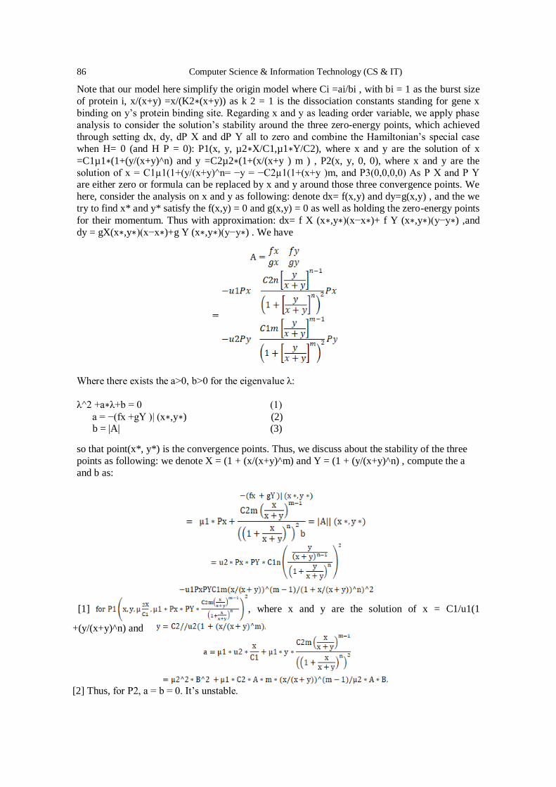
86 Computer Science & Information Technology (CS & IT)
Note that our model here simplify the origin model where Ci =ai/bi , with bi = 1 as the burst size
of protein i, x/(x+y) =x/(K2∗(x+y)) as k 2 = 1 is the dissociation constants standing for gene x
binding on y’s protein binding site. Regarding x and y as leading order variable, we apply phase
analysis to consider the solution’s stability around the three zero-energy points, which achieved
through setting dx, dy, dP X and dP Y all to zero and combine the Hamiltonian’s special case
when H= 0 (and H P = 0): P1(x, y, µ2∗X/C1,µ1∗Y/C2), where x and y are the solution of x
=C1µ1∗(1+(y/(x+y)^n) and y =C2µ2∗(1+(x/(x+y ) m ) , P2(x, y, 0, 0), where x and y are the
solution of x = C1µ1(1+(y/(x+y)^n= −y = −C2µ1(1+(x+y )m, and P3(0,0,0,0) As P X and P Y are either zero or formula can be replaced by x and y around those three convergence points. We
here, consider the analysis on x and y as following: denote dx= f(x,y) and dy=g(x,y) , and the we
try to find x* and y* satisfy the f(x,y) = 0 and g(x,y) = 0 as well as holding the zero-energy points
for their momentum. Thus with approximation: dx= f X (x∗,y∗)(x−x∗)+ f Y (x∗,y∗)(y−y∗) ,and
dy = gX(x∗,y∗)(x−x∗)+g Y (x∗,y∗)(y−y∗) . We have
Where there exists the a>0, b>0 for the eigenvalue λ:
λ^2 +a∗λ+b = 0 (1)
a = −(fx +gY )| (x∗,y∗) (2) b = |A| (3)
so that point(x*, y*) is the convergence points. Thus, we discuss about the stability of the three
points as following: we denote X = (1 + (x/(x+y)^m) and Y = (1 + (y/(x+y)^n) , compute the a
and b as:
[1] , where x and y are the solution of x = C1/u1(1
+(y/(x+y)^n) and
[2] Thus, for P2, a = b = 0. It’s unstable.

Computer Science & Information Technology (CS & IT) 87
[3] for P3 (0, 0, 0, 0), same as P2, a = b = 0 and it’s unstable.
b. Two fixed points for the neuron model
When there is no stimulus, the neuron fire spontaneously(I=0), w< , the two fixed points
is studied through µ (= ) changing with : M0 = (0, ) = (0, arcsin(-w/ ))=(0,-
0.997903) and M1 = (S1, φ1)=(1, pi/2-arcsin(-w/( - S0))) =(1,2.568699) .
Similar to the model a, we denote f(S, φ) = , g(S, φ)
= and the stability of M0 is linear thus can be analysed with the
Jacobian of the coupled (**) at :
we try to find S* and φ* satisfy the f(S*, φ*) = 0 and g(S*, φ*) = 0 as well as holding the zero-
energy points for their momentum. Thus with approximation: dS= fs (S∗, φ∗)(S−S∗)+ fφ (S∗, φ ∗)( φ − φ∗) , and dφ = gs (S∗, φ∗)(S−S∗) + gφ (S∗, φ∗)( φ − φ∗). Where there exists the a>0, b>0
for the eigenvalue λ: λ^2 +a∗λ+b = 0. Thus, a = −(fs +gφ )| (S*,φ∗) = -1+ =-2, b =
|A|=-( + * ) =-(-w+µc (w/ )^2) = -0.323219, leading to λ =
= = {0.817465,-1.361948}, µc
=0.95839
[1] M0 is stable fixed-point for µ<µc, M1 is unstable with φ1> φ0 and S1>S0
[2] M0 is attractor for µ=µc, another fixed point M1 = M0 [3] M0 is unstable fixed-point for µ>µc, M1 is stable with φ1> φ0 and S1<S0
On quantum field, short introduction about two Rydberg here is covered for comparison.
[1] u<< makes it unnecessary to address two atoms separately. Because = = , we can set
d1 = d2 =0 and realize the gate with a)drive a pi-pulse to two atoms->b)pause for dt = φ /u-
>c)drive a pi-pulse again to two atoms. Note that the accumulated phase is sensitive to atomic
distance and the decay probability is approximately pl = 2 φϒ /u
[2]Adiabatical condition for u>> still makes it unnecessary to address two atoms separately.
As = = , d1 = d2 =0 naturally hold due to the slow on time scale given by the two parameter although larger than trap oscillation frequrncy. The detuning includes a Stark shift as
connected to initial state |gg> with energy egg(t) = sgn(d)(|d|-(d^2+2 ^2)^1/2)/2 driven
adiabatically, where d = d- ^2/(4d+2u) while |eg> and |ge> are achieved with eeg(t) =
sgn(d)(|d|-(d^2+ ^2)^1/2)/2 leading to the entanglement phase to beφ(t) = .
[3]u<< generally requires the atoms to be set differently at , differently. But we can still
set dj=0 with the cost of sign change in the wave function through a)drive a pi-pulse to the first
atom->b)a 2pi-pulse to the second c)drive a pi-pulse again to the first atom.

88 Computer Science & Information Technology (CS & IT)
3.2. Dynamics Analysis
a. HMC dynamics for protein and mRNA
Figure 3(a)-(h) transition between mRNA and protein
In the second part here, with regard to the detailed behavior of mRNA and protein dnamics, we look into their momentum and numbers with 6 status (only the firs 2(a)-2(c) and the last 2(d)-2(f)
transition xamples of the origin 3groups*5transition statuses figures) in all are studied detailedly
while the whole data based on 15 status. As we only investigated the positive direction, the red ones (top left) the application on clinical data while green one (top right) in the larger scaled
simulation with more transition status (blue dashed line is the predicted dynamics)..Note that the
persisters and normals are the roles they take in the whole process(considering from bifurcation
to catastrophe and extinction) where here they can be all considered as promoters as their numbers both grows in this process until the last status as their interaction in constant
environment is of our main interest as we mentioned before. Generally, with small change
studied in one status, the trend is more significant than the larger scale transition. For instance, the green simulation are always more sensitive to the momentum change and shows them more
significantly on the cell trajectory comparing to the red clinical transition (we manually break one
clinical status into sub-status in simulations. )
Specifically, in the 1− > 2 transition, the production of the HS 1 is slightly faster than hax1 with
the accelerate from faster to slower as well as the hax1 0 s momentum decreases from fast to
slow while HS 0 1 s momentum increases from fast to slow similarly. The larger scaled simulation show the trend similarly but with larger momentum difference and thus gives out the
curve trajectory instead of straight line in the top left figure; On contrary, in 2− > 3 transition,
both the clinical application and larger simulation give totally the same behavior according to the dynamics, where proteins products faster than mRNA but with similar acceleration. Other
transition can be similarly analysis. Note that from the 4− > 5 of the larger scale simulation, there
starts to show the switching where the protein changes into persisters with degradation instead of production which can be both detected from cell numbers figure in the top left and momentum
figures in the right bottom although the fewer status contained clinical data does not show this
behavior yet. In the last transition status, the switching of proteins becoming into persister is
detected in both clinical process and simulation, where in the clinical data, the momentum change of roteins and mRNA are both linear process while in simulation, the momentum of the mRNA
grows slightly from faster to slower and proteins degradate slightly from faster to slower as well

Computer Science & Information Technology (CS & IT) 89
and in the last short time, proteins go back to normals again which according to the rising number change in the top left and increase in the momentum both relatively to mRNA(left bottom) and
absolutely (right bottom.) )
In the second series of figures2(c),2(f), we compute the mean time to switch approximation with the solution based on mapping to their difference space where we choose the object as 1) sigle
population of mRNA to the end of the transition(top left);2) sigle population of proteins to the
end of the transition (top right); 3) mRNA population to the end status of protein(left bottom) and 4) proteins population to the end status of mRNA.(right bottom.)There gives some different
patterns, as in the 1− > 2 , both the mRNA and proteins has the mean time to switch increase
linearly with their number change while there exists one significatly longer time at 0.4 for the proteins compare to the final status of mRNA and one totally unstable transition recorded; In the
2− > 3 , all the MTS increase linearly with the cell number growth; In the 4− > 5 , as there exhists
the decrease of proteins thus there exhists one negative MTS stands for the status; And in 5−>6 ,
the last status for the proteins again, compared to the final status where the number back to increase, the previous degradation status also leads to the minus MTS but positive to the mRNA
as they both grow in the end. In the last part, Further application using the transition matrix of the
model , we compute some basic markov chain quantities based on the stochastic process as following with the pre-computation result(in availability):
Figure 4 computation of probabilistic safety
In the probabilistic safety computation by finite DTMC abstraction, the computation is based on
the differential cognitive (*) in 2.3.3 with the previous unified matrix of CTMC composed of 6
transition status and 6 time points for each, dX = P(:,2:6) = P(:,1:5);
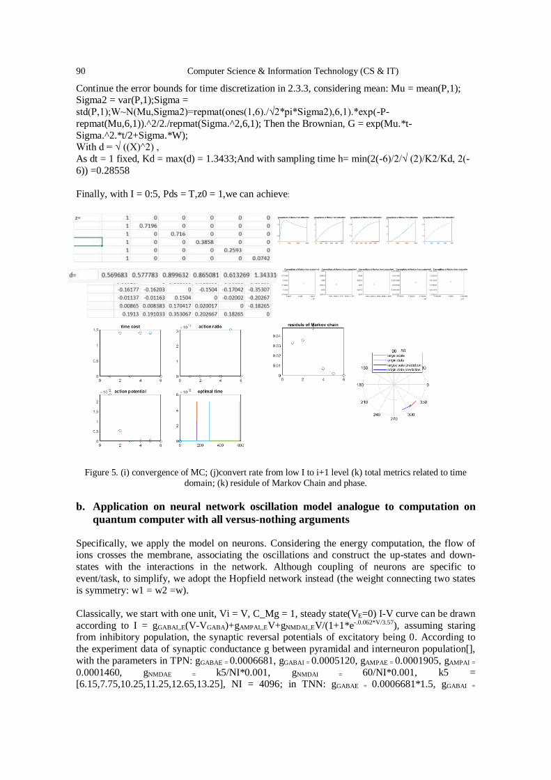
90 Computer Science & Information Technology (CS & IT)
Continue the error bounds for time discretization in 2.3.3, considering mean: Mu = mean(P,1); Sigma2 = var(P,1);Sigma =
std(P,1);W~N(Mu,Sigma2)=repmat(ones(1,6)./√2*pi*Sigma2),6,1).*exp(-P-
repmat(Mu,6,1)).^2/2./repmat(Sigma.^2,6,1); Then the Brownian, G = exp(Mu.*t-
Sigma.^2.*t/2+Sigma.*W); With d = √ ((X)^2) ,
As dt = 1 fixed, Kd = max(d) = 1.3433;And with sampling time h= min(2(-6)/2/√ (2)/K2/Kd, 2(-
6)) =0.28558
Finally, with I = 0:5, Pds = T,z0 = 1,we can achieve:
Figure 5. (i) convergence of MC; (j)convert rate from low I to i+1 level (k) total metrics related to time
domain; (k) residule of Markov Chain and phase.
b. Application on neural network oscillation model analogue to computation on
quantum computer with all versus-nothing arguments
Specifically, we apply the model on neurons. Considering the energy computation, the flow of ions crosses the membrane, associating the oscillations and construct the up-states and down-
states with the interactions in the network. Although coupling of neurons are specific to
event/task, to simplify, we adopt the Hopfield network instead (the weight connecting two states
is symmetry: w1 = w2 =w).
Classically, we start with one unit, Vi = V, C_Mg = 1, steady state(VE=0) I-V curve can be drawn
according to I = gGABAI,,E(V-VGABA)+gAMPAI,,EV+gNMDAI,,EV/(1+1*e-.0.062*V/3.57), assuming staring from inhibitory population, the synaptic reversal potentials of excitatory being 0. According to
the experiment data of synaptic conductance g between pyramidal and interneuron population[],
with the parameters in TPN: gGABAE = 0.0006681, gGABAI = 0.0005120, gAMPAE = 0.0001905, gAMPAI =
0.0001460, gNMDAE = k5/NI*0.001, gNMDAI = 60/NI*0.001, k5 = [6.15,7.75,10.25,11.25,12.65,13.25], NI = 4096; in TNN: gGABAE = 0.0006681*1.5, gGABAI =

Computer Science & Information Technology (CS & IT) 91
0.000512*1.5, gAMPAE = 0.0001905*4, gAMPAI = 0.0001460*4, gNMDAE = 60/NI*0.001, gNMDAI =
k5/NI*0.001, k5 = [6.15,7.75,10.25,11.25,12.65,13.25], NI = 4096
Quantomechanical, the problem of finding stable state can be discussed on kinematic phase:
In a 3D potential ,
where v are single-wells and , are centered around x0 and 0 individually so that the atom
has its state |Ψ+(x)>composed by ψ+, ψ⊥ (ground-state wave functions of with
eigenvalue Ea and v⊥ with eigenvalue E⊥):
(***)
And Ψ+(x) is peaked at the stable point x0 =(x0,0,0), coinsiding with the center of (x) which
can be occupied by the (x). That is in internal state |a>, the atom has the motional state which
after time t still unchanged up to its phase being (Ea+2 E⊥)t/h while in state |b>, sue to the
kinematical evolution of , it will come back to the initial position after oscillating.
If we consider two atoms 1 and 2 both initialized at t =0 with |Ψ+(x)> and Ψ-(x)> same as in
(***) with ψ−(x) ≡ ψ+(−x). Similar as firing rate model R[I], the particles are subject to step
function S(xi) related potentials . The reduced form as 1D two particle
Schrodinger can be achieved with integrating the variables:
And with setting β1 = β2 ≡ β, the symmetric under particle interchange :
, where <ψ−|ψ+> ≪ 1 has been neglected.
This gives out same result that if both atoms are in state |a>, then due to the collisional
phase =0, no interaction takes place.

92 Computer Science & Information Technology (CS & IT)
4. CONCLUSION In general, Hamiltonian markov chain advantage over the markov chain random walk with its
faster convergence. As in 2(i) and 2(j), the convergence(variation to mean) of the markov chain
hamilton is in blue line and the red line for clinical data and simulation on more possible
transition status, giving different convergence but similar phase interval(according to 2(k)), interestingly. The last status transition converge the worst followed by the fist transition. And the
result simulated with more markov chain status converges better than the clinical results. And
according to the convert rate, the mRNA to Protein transfer ratio should be the highest when starting, and goes especially lower in the last two status which is in assistance to the protein
binding as we cut off the process around the convergence point where the two population has
reached metastability. According to the simulation result, the protein has gone through the
switching process changing from normals to persisters and back to normal (bursts in optimal time in 2(j) might also due to the switch.).
Mean while, as the second population providing food(protein) to the other’s binding site and eithr activiate or deactivate it, it works as the extrinsic noise induced the excitability or exhibition of
the other gene. Here, as we choose hax1 and HS 1, they work as promoters for each others. One
noticable computation is the reward computaiton based on stochastic model selection which is useful in predict the possible status of the cell numbers easily with precomputation. And we can
consider correct the transition matrix with simualted clinical tested results to improve the
prediction as well. On the other hand, the most important calculation action potential is easier to
be achieved through Hamilton as we proved with geometric minimum action and stochastic approximation. Ohter methods can cover Hamilton Jacobian matrix, WKB and etc. As we also
improve the algorithm with adding hierarchical markov in calculating number of cells in different
status only record successful move according to the tolerance based on action potential and residual of prediction numbers both, the convergence of the algorithm is guaranteed. And further
research can be conducted on the whole process from bifurcation to catastrophe and extinction as
well. Problem with multi population is also possible. As hax1 is observed to have function in signaling and regulating of genes especially in learning systems and motor related brain function,
this switching model study related to its binding might help to predict the cell numbers and
production or degradation rate especially later with further study into both with promoters and
persisters as to test different drug and their efficiency on the aging process related disease.
In the computation of reachability, the approximation with DTMC mainly compute the kernels of
Brownian with shift, finally discretize the original switching diffusion process. As the DTMC gives out the kernel with probability instead of the ratio, it is then convenient to be written into
transition matrix Pdx which is discretized from Sdx on finite space state and gives out the
reachability with error I/h*(Kdx+exp(-2^n-2^n/2+1)).
As the proof in Appendix, the error bounds with Lipschitz constants converged with prominent
K= mh1+Lh2.And the computed result N*K*dxis here is 0.453 with N = 6, m = L = 2,dx = 0.002
and h1 = 0.001, and h2 = ceil(h2*N)=1.71.
Since the final result of the continuous process is not of probability range thus we normalize it
with P = ratio/sum(ratio) and the DTMC approximation shown in the figure is the approachability(1-safety.) The result of the test tested continuous embedded matrix and h =0,p
=0.0515,ci = -0.7212 , 0.0029,stats = struct with stat: -2.2103( df: 10), do not reject the
hypothesis that the two process. As the final safety consistently for two methods gives highest
concentration for the last state showing the example computation’s direction from off to on, although there is the slight difference that the forth in the continuous process is relative lower
comparing to its other five states as well as the one in the discrete process states. The DTMC

Computer Science & Information Technology (CS & IT) 93
gives strictly increasing concentration from off to on during the 6 states. switching diffusion is a commonly used model in genetic field, not only useful in the transmission of different molecules
but also can be derived into analytical models giving straight transfer information about some
process with either concentration change or energy change.
About the neuron switch model, it is clear that there is similarity between classical computation
and quantum computation with regards to the phase and excitation. This is not surprising since
the process identify the excitation is to compare the spectrum with threshold which basically counting on the transform from time domain to frequency domain and such a process can be
usually realized with operation on exponent computation while the quantum mechanics is origin
from the computation of quantized energy which is also with exponent bases, for instance the most well known poisson distribution and normal distribution as well as the transform as FFT,
the same level of computation at the first place correlate these two. And with our experiment, the
transform can be illustrated with phase initialized at specific state clearly, thus the entanglement
is expressed in quantum computation as well as the classical computation in stability analysis.
As mentioned in the introduction, the similarity exists in the stimulus at hippocampus so as to
simulate spontaneous neuron activities and conducting pi-pulse on atoms with different orders so as to excite it to higher states, this is still not quantitively studied in this paper although some
related phase operations are covered, as of both theoretical and experimental value, worth being
explored more in the future. Many properties of quantum computation with regards to semantics is also of large usage and since neural network is applied frequently in this field, similar
application on quantum computation is also a future direction.
ACKNOWLEDGEMENTS
Although I have graduated with excellence graduates awards, I am still working in the university currently cooperated with university neural dynamic lab. Thanks to all the supervisors and
colleagues I have worked with.
REFERENCES
[1] Freedman,H.I.,Dynamics of simple gene-network motifs subject to extrinsic fluctua-tions,1980
[2] Noufe H. Aljahdaly,Analytical Solutions of a Modified Predator-Prey Model through a New
Ecological Interaction,2019 ensembl,https://www.ensembl.org/index.html
[3] Ingo Lohmar, Baruch Meerson, Switching between phenotypes and population extinction, Racah Institute of Physics, 2018
[4] Daniel Durstewitz1, Jeremy K. Seamans1 and Terrence JRu. Sejnowski1,2, Neurocomputational
models of working memory, 2000
[5] MARCELO CAMPERI, XIAO-JING WANG, A Model of Visuospatial Working Memory in
Prefrontal Cortex: Recurrent Network and Cellular Bistability, 1998
[6] Marta Kwiatkowdka, Gethin Norman, David Parker, Stochastic Model Checking, Oxford, 2019
[7] David Martínez-Rubio, Varun Kanade, Patrick Rebeschini, Decentralized Cooperative Stochastic
Bandits, Oxford, 2005 Paul C Bressloff, Stochastic swiching in biology: from genotype to phenotype,
Department of Mathematics, University of Utah, 2017 Baier, Christel, Principles of Model checking,
Massachusetts Instititute of Technology,2008
[8] Zhu Z, Wang R and Zhu F (2018) The Energy Coding of a Structural Neural Network Based on the Hodgkin–Huxley Model. Front. Neurosci. 12:122. doi: 10.3389/fnins.2018.00122
[9] David Colliaux, Colin Molter, Yoko Yamaguchi, Working memory dynamics and spontaneous
activity in a flip-flop oscillations network model with a Milnor attractor, 2009
[10] D. Jaksch, J.I. Cirac, and P. Zoller, S.L. Rolston, R. Cote and M.D. Lukin , Fast quantum gates for
neutral atoms, 2000, arXiv:quant-ph/0004038v2 , DOI:10.1103/PhysRevLett.85.2208
[11] Samson Abramsky, Lucien Hardy, Logical Bell Inequalities,2012, arXiv:1203.1352v4

94 Computer Science & Information Technology (CS & IT)
[12] Cheng Lv, Xiaoguang Li, Fangting Li, Tiejun Li, Constructing the Energy Landscape for Genetic
Switching System Driven by Intrinsic Noise, Peking University, 2014 [13] C.W. Gardiner, Handbook of Stochastic Methods for Physics, Chemistry and the Natural Sciences,
4th ed, Handbook of Stochastic Methods for Physics, Chemistry and the Natural Sciences, 4th
ed.,Springer, 2009 Alberto Finzi, Thomas Lukasiewicz, Game-Theoretic Agent Programming in GologLuca Cardelli, Marta Kwiatkowowska, Robustness Guarantee.Yasar Demirel, in Non-
equalibrium Thermodynamics (Third Edition), 2014
[14] Matthias Heymann, Eric Vanden-Eijnden, Geometric Minimum Action Metod: A Least Action
Principle on the Space of Curves, Courant Institute, 2007
[15] Approximate Model Checking of Stochastic Hybrid Systems: Alessandro Abate, Joost-Pieter Katoen,
John Lygeros, Maria Prandini. Marta Kwiatkowska, Gethin Norman, Stochastics Model Checking
[16] Author Robert Balson Dingle, Their Derivation and Interpretation, Academic Press, 1973 J.C.,
Gittins, Keble College, Oxford, 2010
[17] Samson Abramsky1 , Rui Soares Barbosa1 , Giovanni Carù1 and Simon Perdrix, A complete
characterization of all-versus-nothing arguments for stabilizer states, 2017,
http://dx.doi.org/10.1098/rsta.2016.0385
[18] Zahid Ur Rehman, Quorum-Quenching Bacteria Isolated From Red Sea Sediments Reduce Biofilm Formation, KAUST,2016
[19] An experimental investigation on the health monitoring of concrete structures using piezoelectric
transducers at various environmental temperatures.
[20] Ali, Isra, Alfarouk, Khalid O., Reshkin, Stephan J., Ibrahium, Muntaser E., Doxycy-cline as Potential
Anti-cancer Agent, Anti Cancer Agents, 2018
[21] Xianjun Cheng , Yue Yuan, Yihong Wang, Rubin Wang, Neural antagonistic mechanism between
default-mode and task-positive networks, 2020, DOI: https://doi.org/10.1016/j.neucom.2020.07.079
[22] G.S. Skone, Irina Voiculescu, Stratagems for effective function evaluation in computa-tional
chemistry, Oxford, 2010
[23] Peter Minary, Charlotte M Deane, Explorong peptide/MHC detachment process using hiearchical
natural move Monte Carlo, Oxford, 2015Biancalani, E. Giamperi, A. Bazzani, G. Catellani, and A. M aritan, Phys.Soc, Jpn., Physics, 2015
[24] D.M. Roma, R.A. P’Flanagan, A.E. Ruckenstein, A.M. Sengupta, R., Optimal path to epigenetic
switching, Rarah Institute of Physics,2015 C HASTE : incorporating a novel multi-scale spatial and
temporal algorithm into a llarge-scale open source librarty B Y M IGUEL O. B ERNABEU 1 , R
AFEL B ORDAS 1 , P RAS P ATHMANATHAN 1 ,J OE P ITT -F RANCIS 1 , J ONATHAN C
OOPER 1 , A LAN G ARNY 2 , D AVIDJ. G AVAGHAN 1 , B LANCA R ODRIGUEZ 1 , J AMES
A. S OUTHERN AND J ONATHAN P. W HITELEY
[25] Chris Holmes Leonhard Held Bayesian Ausiliary Variable Models for Binary and Multinomiak
Regression
[26] Michael Betancourt and Mark Girolami Hamiltonian Monte Carlo for Hierarchical Model
[27] rffany Amariuta, Ynag luo, Steven Gazal, Emma E. Davenport, Bryce van de Geijn, Kazuyoshi
Ishigaki, Alkes L. Price, IMPACT: Genomic Annotation of Cell-State-Specific Regulatory Elements Inferred from the Epigenome of Bound Transcription Factors.
[28] Dynamics statistic Markov chain, Alessandro Abate, Joost-Pieter Katoen, Alexandru Mereacrem

Computer Science & Information Technology (CS & IT) 95
AUTHORS Qin He, Received master degree in data engineering and machine learning with physics
minor. During Bachelor (Maths bachelor in ECUST, student union technology and
entrepreneur department academic division leader, minor in English), did research study in dynamics neuron networks lab, using statistics, data mining basic skills. Minor in
English. In currently master program, doing neuroscience research study related to neuro
imaging, neuron computation, minoring in Physics.) Main field in Mathematics and
programming, with equal interest in other natural science and technology. And due to
past background in machine learning with disciplinary projects, especially related to biomedical and
neuroscience in processing time series, frequency spectrums and Bayes models combining stochastic
process, computational modeling with python, matlab, C/C++ and a little bit C#. Rubin Wang, Received the Ph.D. degree in electronic and mechanical engineering from Nagoya University, Nagoya, Japan, in 1998., He is currently one of the Director of the
Institute of Cognitive Neurodynamics, East China University of Science and Technology,
Shanghai, China. His research interests are in the areas of cognitive neurodynamics, coding
and decoding theory in brain information processing, complexity theory, analysis of
biological neural networks, and computational vision and audition., Dr. Wang serves as the
founding Editor-in-Chief of Cognitive Neurodynamics.
Xiaochuan Pan, Received the Ph.D. degree in biophysics, University of Chinese Academy
of Sciences, in 1997.,He is currently one of the Director of the Institute of Cognitive
Neurodynamics, East China University of Science and Technology, Shanghai, China. His
research interests are in the areas of cognitive neurodynamics, coding and decoding theory in brain information processing, complexity theory, analysis of biological neural networks,
and computational vision and audition. Dt.Pan is professional at behaviour models related
to deduction, conditional random dynamics and optimization.
APPENDIX
Because of paper limit see:
https://github.com/LilyHeAsamiko/QC/blob/master/UAE_ADCO(2021.02.21_02.17)/appendix%20of%20
Genetic%20Switches%20between%20two%20population%20with%20regards%20to%20mRNA%20and%
20proteins%20applying%20Markov%20Chain%20Stochastic%20Model%20Check_cor.docx
© 2021 By AIRCC Publishing Corporation. This article is published under the Creative Commons Attribution (CC BY) license.

AUTHOR INDEX
Hikaru Morita 01
Ismailova Aisulu 17
Juan Zhao 35, 53
Qin He 71
Rubin Wang 71
Saeko Matsuura 01
Shopagulov Olzhas 17
Tretyakov Igor 17
Xiaochuan Pan 71
Zhitang Li 35, 53