COMPUTER PROGRAM FOR SOLVING GROUND-WATER FLOW … · by the preconditioned conjugate gradient...
37
COMPUTER PROGRAM FOR SOLVING GROUND-WATER FLOW EQUATIONS BY THE PRECONDITIONED CONJUGATE GRADIENT METHOD By Logan K. Kuiper U.S. GEOLOGICAL SURVEY Water-Resources Investigations Report 87-4091 Austin, Texas 1987
Transcript of COMPUTER PROGRAM FOR SOLVING GROUND-WATER FLOW … · by the preconditioned conjugate gradient...
COMPUTER PROGRAM FOR SOLVING GROUND-WATER FLOW EQUATIONS BY THE PRECONDITIONED CONJUGATE GRADIENT METHOD
By Logan K. Kuiper
U.S. GEOLOGICAL SURVEY
Water-Resources Investigations Report 87-4091
Austin, Texas 1987
DEPARTMENT OF THE INTERIOR
DONALD PAUL HODEL, Secretary
U.S. GEOLOGICAL SURVEY
Dallas L. Peck, Director
For more information write to:
Project ChiefU.S. Geological SuveyGulf Coast RASAN. Shore Plaza Bldg., Rm. 10455 North Interregional Hwy.Austin, Texas 78702
Copies of this report can be purchased from:
U.S. Geologicl Survey Books and Open-File Reports Federal Center, Bldg., 41 Box 25425Denver, Colorado 80225 Telephone (303) 236-7476
CONTENTS
Page
Ab s t r ac t 1Introduction 1Preconditioned conjugate gradient package 2
Description and use 2Input instructions 10Sample input to preconditioned conjugate gradient package 12Module documentation for the preconditioned conjugate gradientpackage 13
PCG1AL 13Narrative 13Flow chart 14Program listing 14List of variables 16
PCG1RP 17Narrative 17Flow chart 17Program listing 18List of variables 18
PCG1AP 19Narrative 19Flow chart 22Program listing 23List of variables 31
References 34
ILLUSTRATIONS
Page
Figure 1. Correspondence between the finite-differenceequations and the matrix equation for a gridwith three rows, two columns, and two layers 4
Figure 2. Structure of coefficient matrix showing nonzero diagonals
Figure 3. Flowchart showing major elements of module PCG1AP and related parts of the main program of the modular model
TABLES
Page
Table 1. ITYP control of v and u iterations 21
111
COMPUTER PROGRAM FOR SOLVING GROUND-WATER FLOW EQUATIONS
BY THE PRECONDITIONED CONJUGATE GRADIENT METHOD
By Logan K. Kuiper
ABSTRACT
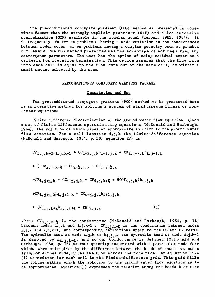
This report documents a numerical code for use with the U.S. Geological Survey modular three-dimensional finite-difference ground-water flow model. The code uses the preconditioned conjugate gradient method for the solution of the finite difference approximating equations generated by the modular flow model. These equations are a system of simultaneous linear equations except when the river, drain, or evapotranspiration packages of the modular model are being used, in which case they are a system of simultaneous nonlinear equations. When these equations are linear, they are solved by the basic preconditioned conjugate gradient method as available in the literature. Five preconditioning types may be chosen: three different types of incomplete Choleski, point Jacobi, or block Jacobi. When the approximating equations are nonlinear, the solution method is that of Picard preconditioned conjugate gradient with the same preconditioning choices. Either a head change or residual error criteria may be used as an indicator of solution accuracy and iteration termination.
The use of the computer program that performs the calculations in the numerical code is emphasized. Detailed instructions are given for using the computer program, including data entry formats and the method of linking the program into the modular model. A sample data listing and listing of the Fortran program are included.
INTRODUCTION
This report documents a numerical code for use with the U.S. Geological Survey modular three-dimensional finite-difference ground-water flow model (McDonald and Harbaugh, 1984). The code uses the preconditioned conjugate gradient method for the solution of the finite difference approximating equa tions generated by the modular flow model. These equations are a system of simultaneous linear equations except when the river, drain, or evaporation packages of the modular model are being used, in which case they are a system of simultaneous nonlinear equations. When these equations are linear, they are solved by the basic preconditioned conjugate gradient method as available in the literature. Five preconditioning types may be chosen: three different types of incomplete Choleski, point Jacobi, or block Jacobi. When the approxi mating equations are nonlinear the solution method is that of Picard precondi tioned conjugate gradient with the same preconditioning choices. Either a head change or residual error criteria may be used as an indicator of solution accuracy and iteration termination.
The preconditioned conjugate gradient (PCX?) method as presented is some times faster than the strongly implicit procedure (SIP) and slice-succesive overrelaxation (SOR) available in the modular model (Kuiper, 1981, 1987). It is frequently faster on problems having a wide variation in the conductances between model nodes, or on problems having a complex geometry such as pinched out layers. The PCG method presented has the advantage of not requiring any convergence parameters. The user has the option of using residual error as a criteria for iteration termination. This option assures that the flow rate into each cell is equal to the flow rate out of the same cell, to within a small amount selected by the user.
PRECONDITIONED CONJUGATE GRADIENT PACKAGE
Description and Use
The preconditioned conjugate gradient (PCG) method to be presented here is an iterative method for solving a system of simultaneous linear or non linear equations.
Finite difference discretization of the ground-water flow equation gives a set of finite difference approximating equations (McDonald and Harbaugh, 1984), the solution of which gives an approximate solution to the ground-water flow equation. For a cell location i.j.k the finite-difference equation (McDonald and Harbaugh, 1984, p. 30, equation 27) is:
HCOFifj>k)hif
+CR
.j.k (1)
where CV£4 jk_^ is the conductance (McDonald and Harbaugh, 1984, p. 16) between nodes i,j,k and i,j,k-l , CV^ j k+v is the conductance between nodes i,j,k and i,j,k+l, and corresponding definitions apply to the CC and CR terms. The hydraulic head at node i,j,k is h^ j k, the hydraulic head at node i,j,k-l is denoted by h^ ^ k-l» and so on. Conductance is defined (McDonald and Harbaugh, 1984, p. 16) as that quantity associated with a particular node face which, when multiplied by the difference between the heads of those two nodes lying on either side, gives the flow across the node face. An equation like (1) is written for each cell in the finite-difference grid. This grid fills the volume within which the solution to the ground-water flow equation is to be approximated. Equation (1) expresses the relation among the heads h at node
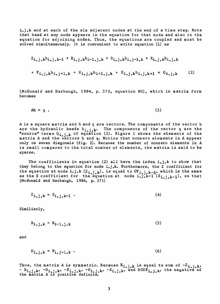
i,j,k and at each of the six adjacent nodes at the end of a time step. Note that head at any node appears in the equation for that node and also in the equation for adjoining nodes. Thus, the equations are coupled and must be solved simultaneously. It is convenient to write equation (1) as
(2)
(McDonald and Harbaugh, 1984, p. 370, equation 80), which in matrix form becomes
Ah = q . (3)
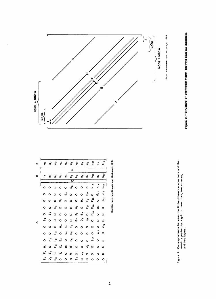
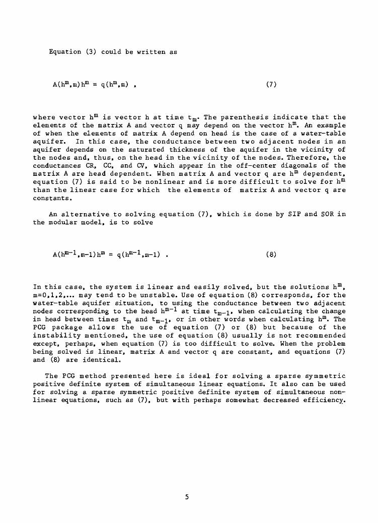
A is a square matrix and h and q are vectors. The components of the vector h are the hydraulic heads hi t i t k' The components of the vector q are the "source" terms Qi f i k of equation (2). Figure 1 shows the elements of the matrix A and the vectors h and q. Notice that nonzero elements in A appear only on seven diagonals (fig. 2). Because the number of nonzero elements in A is small compared to the total number of elements, the matrix is said to be sparse.
The coefficients in equation (2) all have the index i»j,k to show that they belong to the equation for node i.j.k. Furthermore, the Z coefficient for the equation at node i,j,k (Zi f j fk)i is equal to CVj^ -i f k-%» which is the same as the S coefficient for the equation at node i,j,k-l (S-j^ tk_;L), so that (Mcdonald and Harbaugh, 1984, p. 371)
zi.j.k= Si.j.k-l . (4)
Similiarly,
Bi.j.k = Hi-i.j.k (5)
and
Thus, the matrix A is symmetric. Because E^.: k is equal to sum of ~z i t j >k i- B.; -; V, -D-- 4 I,, -FH- i L., -H-- u ],, -Si« -; L., and HCOF-- 4 ],, the negative of L »j»*-. iij»«- . i^j*^ f»J» K- J-ij»«- i»ji«- °the matrix A is positive definite.
E,
F,
H,
O
O
O
St
O
O
O
O
O
D2
E2
O
H2
O
O
O
S2
O
O
O
O
B3
O
E3
F3
H3
O
O
O
S3
O
O
O
O
B4
D4
E4
O
H4
O
O
O
S4
O
O
O
O
B5
O
E5
F5
O
O
O
O
S5
O
O
O
O
B6
D6
E6
O
O
O
O
O
S6
Z7
O
O
O
O
O
E7
F7
H7
O
O
O
O
28
O
O
O
O
DB
E8
O
H8
O
O
O
O
Zg
O
O
O
B
g
O
Eg
Fg
Hg
O
0
0
0
Z10
0
0
0
B
10
D10
E
10 0
H
10
O
O
O
O
Zn
O
O
O
81
1 O
En
F1
t,
O
O
O
O
O
Z12
O
O
O
B
12
D12
E
12
X
hi h2 r»3 h4 Us "6 h7
*a hg h10 nil
h12
=
Vqa q3 Q
4 q5 q6 q? qa q9 qio
«iii
q12
Mo
difi
ed
fro
m
Mac
Oon
ald
and
Har
baug
h,
1984
Fig
ure
1 . C
orr
esp
ondence
bet
wee
n th
e fin
ite-d
iffere
nce
equ
atio
ns a
nd t
he
mat
rix e
quat
ion
for
a gr
id o
f th
ree
row
s, t
wo
col
umns
, an
d tw
o la
yers
.
NCOL* NROW
NCOL
NCOL
NCOL * NROW
Fro
m
MacO
onald
an
d H
arb
au
gh
, 19
84
Figu
re 2
. S
tru
ctu
re o
f co
effi
cien
t m
atri
x sh
owin
g no
nzer
o di
agon
als.
Equation (3) could be written as
A(hm.m)hm = q(hm ,m) , (7)
where vector hm is vector h at time tm . The parenthesis indicate that the elements of the matrix A and vector q may depend on the vector hm. An example of when the elements of matrix A depend on head is the case of a water-table aquifer. In this case, the conductance between two adjacent nodes in an aquifer depends on the saturated thickness of the aquifer in the vicinity of the nodes and, thus, on the head in the vicinity of the nodes. Therefore, the conductances CR, CC, and CV, which appear in the off-center diagonals of the matrix A are head dependent. When matrix A and vector q are hm dependent, equation (7) is said to be nonlinear and is more difficult to solve for hm than the linear case for which the elements of matrix A and vector q are constants.
An alternative to solving equation (7), which is done by SIP and SOR in the modular model, is to solve
(8)
In this case, the system is linear and easily solved, but the solutions h m , m=0,l,2,... may tend to be unstable. Use of equation (8) corresponds, for the water-table aquifer situation, to using the conductance between two adjacent nodes corresponding to the head hm~l at time tm_^, when calculating the change in head between times tm and tm-l» or in other words when calculating hm . The PCG package allows the use of equation (7) or (8) but because of the instability mentioned, the use of equation (8) usually is not recommended except, perhaps, when equation (7) is too difficult to solve. When the problem being solved is linear, matrix A and vector q are constant, and equations (7) and (8) are identical.
The PCG method presented here is ideal for solving a sparse symmetric positive definite system of simultaneous linear equations. It also can be used for solving a sparse symmetric positive definite system of simultaneous non linear equations, such as (7), but with perhaps somewhat decreased efficiency.
An important part of the PCG method presented here is the basic PCG method for sparse symmetric positive definite linear systems, as taken from the literature (Van Der Vorst. 1982):
EV = , (9)
- Xy + ayPV . (10)
= rv -
Bv - __________ . and (12)
Pv+1 ~ K rv+l + BvPv (13)
is the inner product of the vectors x and y. Iteration of equations (9) through (13) using v=l,2.... . and using r^=b-Ax^, p^=K~^r^, and some initial choice x^ for the solution vector gives an approximate solution to the matrix equation Ax=b. where A is a N by N symmetric positive definite matrix. The residual error vector is r=b-Ax. Matrix K is called a preconditioning or splitting matrix. It is chosen to be as nearly equal to A as possible but readily invertible. The PCG package allows for five choices of the precondi tioning matrix. The first three choices for matrix K (corresponding to NPCOND=l,2.and 3) are three different types of incomplete Choleski factoriza tion (Kershaw. 1978). where the first two differ only in the manner of treating inactive nodes. The fourth choice (NPCOND=4) is point Jacobi (Hageman and Young, 1981) for which matrix K is simply the diagonal of the matrix A. The fifth choice (NPCOND=5) is block Jacobi for which matrix K is the diagonal and the two off-center diagonals adjacent to the center diagonal of A.
The basic PCG method in equations (9) through (13) is part of the PCG method presented here. The solution of equation (7), hm , is the head, h, at time tm. The PCG method presented here finds an approximation to hm itera- tively. Let these sucessive approximations to hm be denoted by h s m , s=l,2,...,sm. Let hsm m denote that iteration taken to be a satisfactory approximate solution to hm. The first estimate for hm+^, h^ m+^, is taken to be hsm m . To explain the way succesive iterations hs m are chosen, it is necessary to break the index s into two indices, u and v, where index v changes fastest. The indices u and v go from 1 to urn, and from 1 to vm(u) respectively. The procedure for finding the approximate solution hsmm, to hm is:
Approximately solve
A(hu>1 m ,m)hum = q(hUjl m ,m) . for u=l,2,...,um , (14)
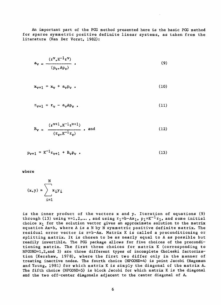
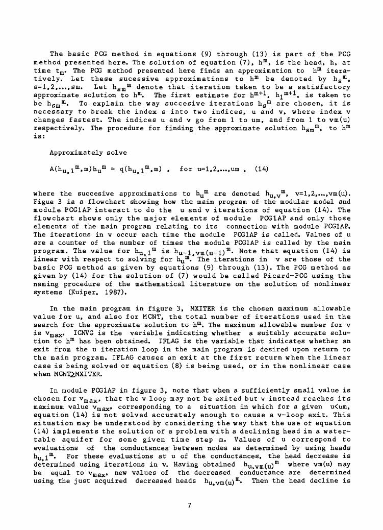
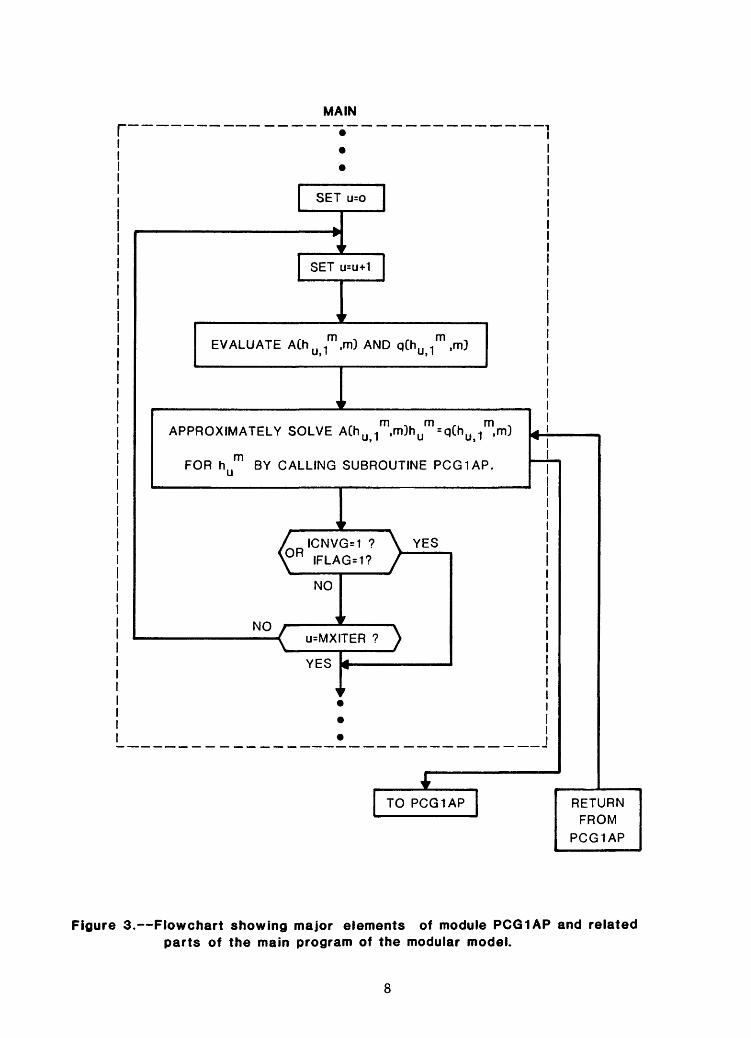
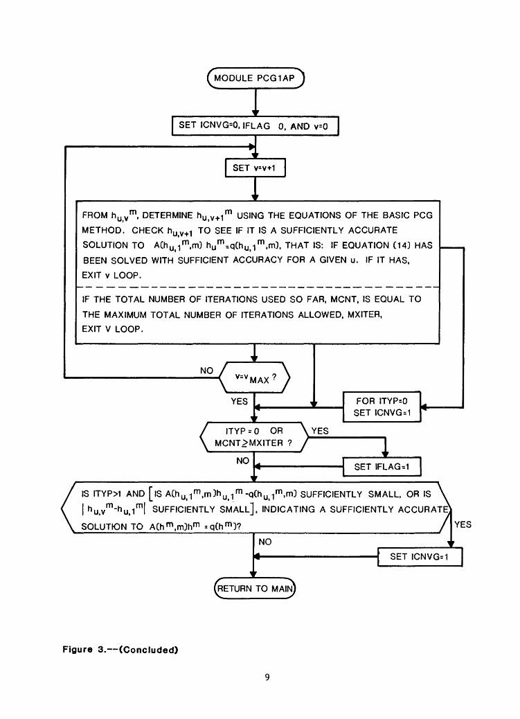
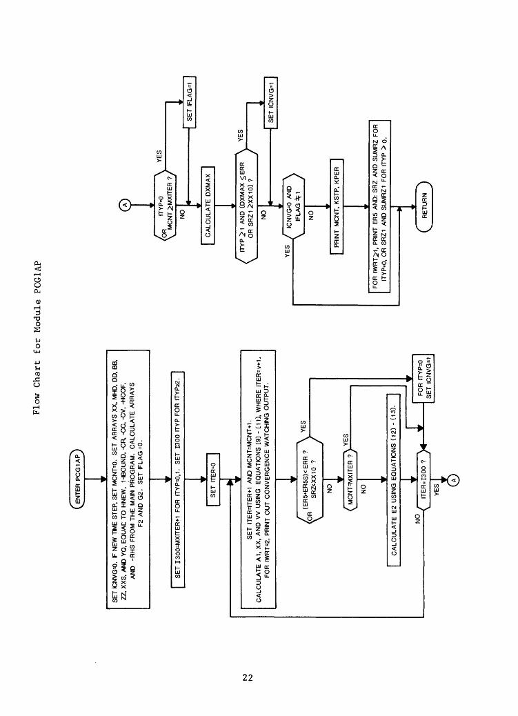
where the succesive approximations to hum are denoted hu vm , v=l,2,...,vm(u). Figue 3 ia a flowchart showing how the main program of the modular model and module PCG1AP interact to do the u and v iterations of equation (14). The flowchart shows only the major elements of module PCG1AP and only those elements of the main program relating to its connection with module PCG1AP. The iterations in v occur each time the module PCG1AP is called. Values of u are a counter of the number of times the module PCG1AP is called by the main program. The value for hUj ^ m is hu_i jVm(u-l) m * Note that equation (14) is linear with respect to solving for hum. The iterations in v are those of the basic PCG method as given by equations (9) through (13). The PCG method as given by (14) for the solution of (7) would be called Picard-PCG using the naming procedure of the mathematical literature on the solution of nonlinear systems (Kuiper, 1987).
In the main program in figure 3, MXITER is the chosen maximum allowable value for u, and also for MCNT, the total number of iterations used in the search for the approximate solution to hm . The maximum allowable number for v is vmax. ICNVG is the variable indicating whether a suitably accurate solu tion to hm has been obtained. IFLAG is the variable that indicates whether an exit from the u iteration loop in the main program is desired upon return to the main program. IFLAG causes an exit at the first return when the linear case is being solved or equation (8) is being used, or in the nonlinear case when MCNT^MXITER.
In module PCG1AP in figure 3, note that when a sufficiently small value is chosen for vmax> that the v loop may not be exited but v instead reaches its maximum value vmax, corresponding to a situation in which for a given u<um, equation (14) is not solved accurately enough to cause a v-loop exit. This situation may be understood by considering the way that the use of equation (14) implements the solution of a problem with a declining head in a water- table aquifer for some given time step m. Values of u correspond to evaluations of the conductances between nodes as determined by using heads hu i m. For these evaluations at u of the conductances, the head decrease is determined using iterations in v. Having obtained ^u,vm(u) m where vm(u) may be equal to vmax, new values of the decreased conductance are determined using the just acquired decreased heads nu,vm(u) m' Then the head decline is
MAIN
"EVALUATE ACh, .m) AND qCh,,
U, I U,
APPROXIMATELY SOLVE
FOR h ym BY CALLING SUBROUTINE PCG1AP.
/ ICNVG=1 ? \ \OR FLAG-1? /
YES
NO
NOJ=MXITER ?
YES
TO PCG1AP RETURNFROM
PCG1AP
Figure 3. Flowchart showing major elements of module PCG1AP and related parts of the main program of the modular model.
(MODULE PCG1APJ
SET ICNVG=0, IFLAG 0, AND v=0
SET v=v-H
FROM h U(V m, DETERMINE h UiV+1 m USING THE EQUATIONS OF THE BASIC PCG
METHOD. CHECK h U|VH-1 TO SEE IF IT IS A SUFFICIENTLY ACCURATE
SOLUTION TO A(h U|1 m,m) hu m a qCh Ui1 m ,m), THAT IS: IF EQUATION (14) HAS
BEEN SOLVED WITH SUFFICIENT ACCURACY FOR A GIVEN u. IF IT HAS,
EXIT v LOOP.
IF THE TOTAL NUMBER OF ITERATIONS USED SO FAR, MCNT, IS EQUAL TO
THE MAXIMUM TOTAL NUMBER OF ITERATIONS ALLOWED, MXITER,
EXIT V LOOP.
INO V=V MAX ?
YES FOR ITYP=0 SET ICNVG=1
ITYP = 0 OR MCNT>MXITER ?
YES
NO1
SET IFLAG =1
IS ITYP>1 AND [iS A(h uj m ,m)h uj m -q(h ujm ,m) SUFFICIENTLY SMALL, OR IS \rv* *v* I ' "1 \
k
h 'H-h l 'M 1 'u,v n u, 1 I
SOLUTION TO
SUFFICIENTLY SMALL], INDICATING A SUFFICIENTLY ACCURATE^
A(h m,m)hm =qCh m )? / YE
i
NO
« t
(RETURN TO MAIN)
\ 'SET ICNVG=1
Figure 3. (Concluded)
redetermined corresponding to these new decreased values for the conductances. The process continues in this manner. Therefore, one need not necessarily solve for head declines accurately for a given u<um because the conductances corresponding to this value for u are too large anyway. Two approaches are thus allowed: for a given evaluation of the conductances corresponding to hu i m , either solve for the head accurately enough to meet some accuracy criteria, or just stop the iteration in v at some vmax . In many cases, problems which are nearly linear are solved with a smaller total number of iterations by choosing a large value for vmax resulting in the program exiting the v loop. On the other hand, extremely nonlinear problems are solved more readily by choosing vmax to be small.
In module PCG1AP, the choice of vmax is controlled by the users choice of the variable ITYP. For a choice of ITYP=0, equation (8), or in the linear case the equivalent equation (7), is solved. For choices of ITYP^.1, equation (7) is solved by means of equation (14), corresponding to the nonlinear case, using vmax=MXITER when ITYP=1, and vmax=ITYP-l when ITYP12.
Input Instructions
The Preconditioned Conjugate Gradient (PCG) Package reads values from the unit specified in IUNIT(13) in the Basic (BAS) Package of the modular model.
For each simulation:
PCG1AL
1. Data: MXITER NPCOND ITYP Format: 110 110 110
PCG1AL
2. Data: HCLOSE RESERR IWRT Format: F10.0 F10.0 110
Read only if IWRT=2:
3. Data: NU1(I),I=1,9 Format: (914)
Explanation of Fields Used in Input Instructions
MXITER
is the maximum total number iterations allowed in an attempt to solve the system of finite difference equations. One hundred iterations should be sufficient for most (ITYP=0) problems.
10
NPCOND--
has the values 1 to 5 corresponding to the five preconditioning types which may be chosen. The first three are incomplete Choleski, the fourth is point Jacobi, and the fifth is block Jacobi. NPCOND equal 1 or 3 are common choices. On rare occasions NPCOND equal 4 or 5 could be faster than 1 or 3. NPCOND equal 2 is at present identical to NPCOND equal 1, but may be changed at a later time. The advised procedure is to use either NPCOND equal 1 or 3, or use both and compare computation times if the model is going to be run many times and computation time is important. NPCOND equal 1 is usually a bit slower than NPCOND equal 3, but it is also more stable. For those who do not wish to experiment with NPCOND, the best choice is 1.
ITYP
is a flag indicating the type of problem solved:
0 - linear problems: LAYCON=0; river, drain, or evaporation packages are not being used. Also for nonlinear problems to be solved with equa tion (8). Such equation (8) solutions for nonlinear problems may be inaccurate and are therefore not recommended unless a solution cannot be obtained using ITYP^.1 or SIP. For equation (8) solutions, the usual budget and flowchart calculations printed by the modular model may be innacurate, and cannot be used as a measure of solution accuracy. See page 20 for more detail.
1 - nonlinear problems with weakly nonlinear conditions.
2 - nonlinear problems with strongly nonlinear conditions. If you do not know how nonlinear the problem is, use ITYP equal 1 and 2 and compare results. See table 1 on page 21 for more detail.
HCLOSE
is the head change criteria for convergence. When the maximum absolute head change for all nodes from the last iteration(s) is less than HCLOSE, iteration is terminated.
RESERR--
is the residual error criteria for convergence. Residual error is the flow rate into a variable head cell minus the flow rate out of the cell. When the maximum, over all the variable head cells in the modeled region, of the absolute values of the residual errors for each of the variable head cells is less than RESERR, iteration is terminated.
Both HCLOSE and RESERR may be used concurrently in which case both have nonzero values. Set HCLOSE=0 if you want to use only RESERR, and vise-versa.
11
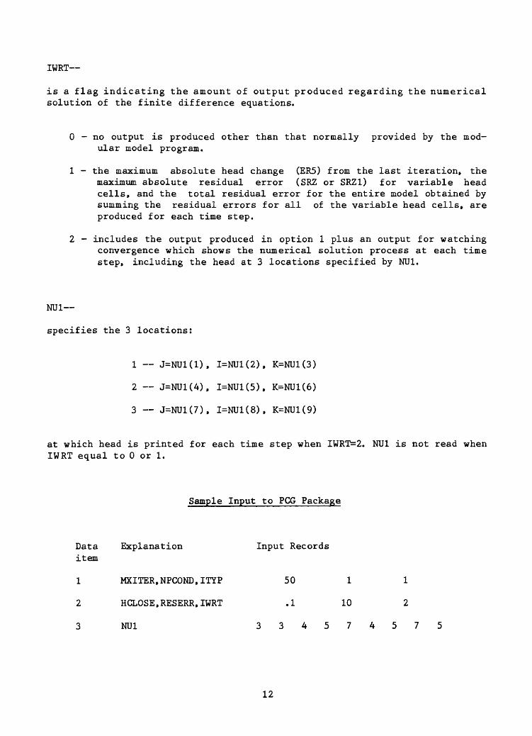
IWRT
is a flag indicating the amount of output produced regarding the numerical solution of the finite difference equations.
0 - no output is produced other than that normally provided by the mod ular model program.
1 - the maximum absolute head change (ER5) from the last iteration, the maximum absolute residual error (SRZ or SRZ1) for variable head cells, and the total residual error for the entire model obtained by summing the residual errors for all of the variable head cells, are produced for each time step.
2 - includes the output produced in option 1 plus an output for watching convergence which shows the numerical solution process at each time step, including the head at 3 locations specified by NU1.
NU1
specifies the 3 locations:
1 J=NU1(1), I=NU1(2), K=NU1(3)
2 J=NU1(4), I=NU1(5), K=NU1(6)
3 J=NU1(7), I=NU1(8), K=NU1(9)
at which head is printed for each time step when IWRT=2. NU1 is not read when IWRT equal to 0 or 1.
Sample Input to PCG Package
Data Explanation Input Records item
1 MXITER.NPCOND.ITYP 50 1 1
2 HCLOSE.RESERR.IWRT .1 10 2
3 NU1 334574575
12
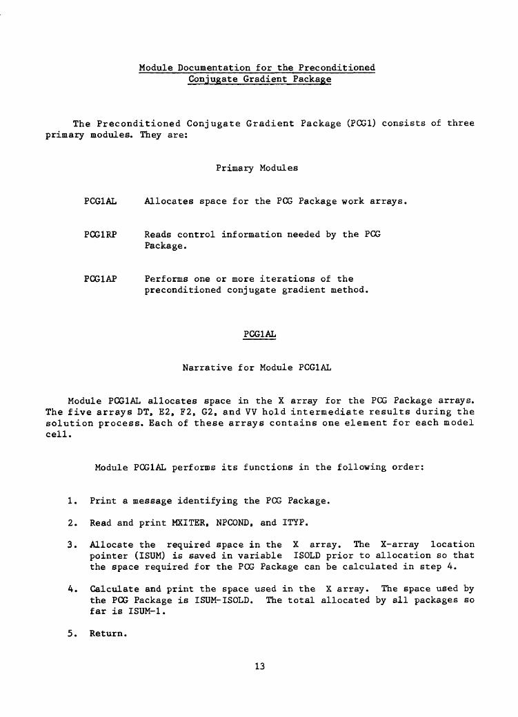
Module Documentation for the Preconditioned Conjugate Gradient Package
The Preconditioned Conjugate Gradient Package (PCG1) consists of three primary modules. They are:
Primary Modules
PCG1AL Allocates space for the PCG Package work arrays,
PCG1RP Reads control information needed by the PCG Package.
PCG1AP Performs one or more iterations of thepreconditioned conjugate gradient method.
PCG1AL
Narrative for Module PCG1AL
Module PCG1AL allocates space in the X array for the PCG Package arrays. The five arrays DT, E2, F2, G2, and VV hold intermediate results during the solution process. Each of these arrays contains one element for each model cell.
Module PCG1AL performs its functions in the following order:
1. Print a message identifying the PCG Package.
2. Read and print MXITER. NPCOND. and ITYP.
3. Allocate the required space in the X array. The X-array location pointer (ISUM) is saved in variable ISOLD prior to allocation so that the space required for the PCG Package can be calculated in step 4.
4. Calculate and print the space used in the X array. The space used by the PCG Package is ISUM-ISOLD. The total allocated by all packages so far is ISUM-1.
5. Return.
13
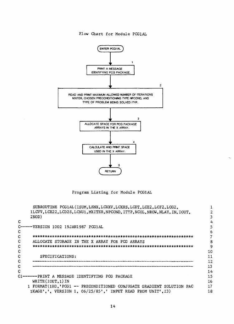
Flow Chart for Module PCGIAL
QENTER PCG1AL
PRINT A MESSAGE IDENTIFYING PCG PACKAGE.
READ AND PRINT MAXIMUM ALLOWED NUMBER OF ITERATIONSMXITER, CHOSEN PRECONDITIONING TYPE NPCOND. AND
TYPE OF PROBLEM BEING SOLVED ITYP.
ALLOCATE SPACE FOR PCG PACKAGE ARRAYS IN THE X ARRAY.
CALCULATE AND PRINT SPACE
USED IN THE X ARRAY.
C RETURN J
Program Listing for Module PCGIAL
Cc Cc c c c c c c cCl-
SUBROUTINE PCGIAL (ISUM,LENX,LCXXV,LCXXS,LCDT,LCE2,LCF2,LCG2, ILCVV,LCE22,LCD2S,LCNU1,MXITER.NPCOND,ITYP,NCOL,NROW,NLAY,IN,IOUT, 2NOD)
VERSION 1002 19JAN1987 PCGIAL
ALLOCATE STORAGE IN THE X ARRAY FOR PCG ARRAYS
SPECIFICATIONS:
PRINT A MESSAGE IDENTIFYING PCG PACKAGEWRITE(IOUT,1)IN
1 FORMAT(1HO, 1 PCG1 PRECONDITIONED CONJUGATE GRADIENT SOLUTION PAG 1KAGE',', VERSION 1, 06/25/85',' INPUT READ FROM UNIT',13)
123456789
101112131415161718
14
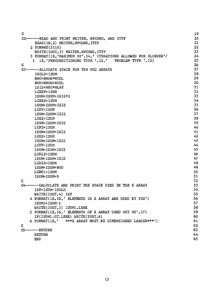
C 19C2 READ AND PRINT MXITER, NPCOND, AND ITYP 20
READ(IN,2) MXITER,NPCOND,ITYP 212 FORMAT(3I10) 22
WRITE(IOUT,3) MXITER,NPCOND,ITYP 233 FORMAT(IX,'MAXIMUM OF',14,' ITERATIONS ALLOWED FOR CLOSURE 1 / 24
1 IX,'PRECONDITIONING TYPE ',12,' PROBLEM TYPE ',12) 25C 26 C3 ALLOCATE SPACE FOR THE PCG ARRAYS 27
ISOLD=ISUM 28NRC=NROW*NCOL 29NOD=NROW+NCOL 30ISIZ=NRC*NLAY 31LCXXV=ISUM 32ISUM=ISUM+ISIZ*2 33LCXXS=ISUM 34ISUM=ISUM+ISIZ 35LCDT=ISUM 36ISUM=ISUM+ISIZ 37LCE2=ISUM 38ISUM=ISUM+ISIZ 39LCF2=ISUM 40ISUM=ISUM+ISIZ 41LCG2=ISUM 42ISUM=ISUM+ISIZ 43LCW=ISUM 44ISUM=ISUM+ISIZ 45LCE22=ISUM 46ISUM=ISUM+ISIZ 47LCD2S=ISUM 48ISUM=ISUM+NOD 49LCNU1=ISUM 50ISUM=ISUM+9 51
C 52 C4 CALCULATE AND PRINT THE SPACE USED IN THE X ARRAY 53
ISP=ISUM-ISOLD 54WRITE(IOUT,4) ISP 55
4 FORMAT(IX,16,' ELEMENTS IN X ARRAY ARE USED BY PCG 1 ) 56ISUM1=ISUM-1 57WRITE(IOUT,5) ISUM1.LENX 58
5 FORMAT(IX,16,' ELEMENTS OF X ARRAY USED OUT OF 1 ,17) 59IF(ISUMl.GT.LENX) WRITE(IOUT,6) 60
6 FORMAT(1X,' ***X ARRAY MUST BE DIMENSIONED LARGER*** 1 ) 61C 62C5 RETURN 63
RETURN 64END 65
15
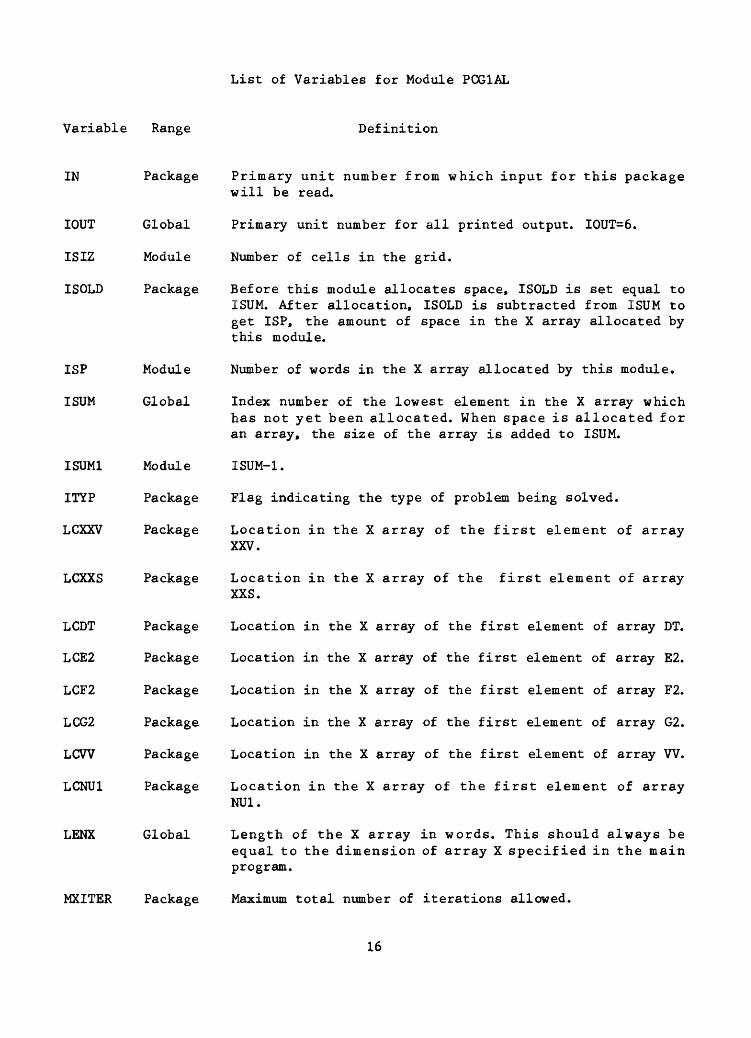
List of Variables for Module PCG1AL
Variable Range Definition
IOUT Global
ISIZ Module
ISOLD Package
IN Package Primary unit number from which input for this packagewill be read.
Primary unit number for all printed output. IOUT=6.
Number of cells in the grid.
Before this module allocates space, ISOLD is set equal to ISUM. After allocation, ISOLD is subtracted from ISUM to get ISP, the amount of space in the X array allocated by this module.
ISP Module Number of words in the X array allocated by this module.
ISUM Global Index number of the lowest element in the X array whichhas not yet been allocated. When space is allocated for an array, the size of the array is added to ISUM.
ISUM-1.
Flag indicating the type of problem being solved.
Location in the X array of the first element of array XXV.
LCXXS Package Location in the X array of the first element of arrayXXS.
Location in the X array of the first element of array DT.
Location in the X array of the first element of array E2.
Location in the X array of the first element of array F2.
Location in the X array of the first element of array G2.
Location in the X array of the first element of array W.
Location in the X array of the first element of array NU1.
LENX Global Length of the X array in words. This should always beequal to the dimension of array X specified in the main program.
MXITER Package Maximum total number of iterations allowed.
ISUM1
ITYP
LCXXV
Module
Package
Package
LCDT
LCE2
LCF2
LCG2
LCW
LCNU1
Package
Package
Package
Package
Package
Package
16
NCOL Global
NLAY Global
NPCOND Module
NRC Module
NROW Global
Number of columns in the grid.
Number of layers in the grid.
Has the values 1 to 5 correspondingto the 5 precondi tioning types.
Number of cells in a layer.
Number of rows in the grid.
PCG1RP
Narrative for Module PCG1RP
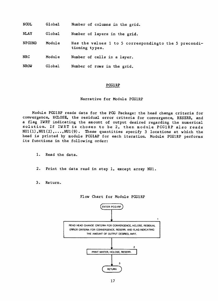
Module PCG1RP reads data for the PCG Package: the head change criteria for convergence. HCLOSE, the residual error criteria for convergence, RESERR, and a flag IWRT indicating the amount of output desired regarding the numerical solution. If IWRT is chosen to be 2, then module PCG1RP also reads NU1(1),NU1(2),...,NU1(9) . These quantities specify 3 locations at which the head is printed by module PCG1AP for each iteration. Module PCG1RP performs its functions in the following order:
1. Read the data.
2. Print the data read in step 1, except array NU1
3. Return.
Flow Chart for Module PCG1RP
.ENTER PCG1RP
READ HEAD CHANGE CRITERIA FOR CONVERGENCE, HCLOSE, RESIDUAL
ERROR CRITERIA FOR CONVERGENCE, RESERR, AND FLAG INDICATING
THE AMOUNT OF OUTPUT DESIRED, IWRT.
PRINT MXITER, HCLOSE, RESERR.
C RETURN J
17
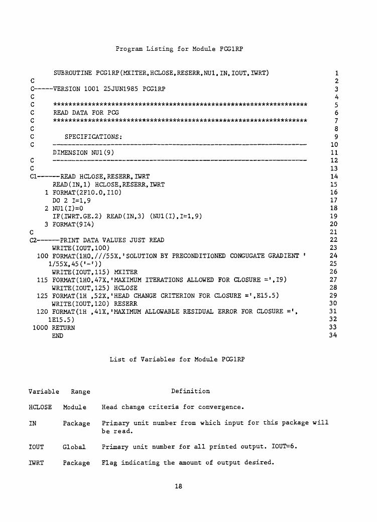
Program Listing for Module PCGIRP
SUBROUTINE PCGIRP(MXITER.HCLOSE,RESERR.NUI.IN.IOUT.IWRT) 1C 2C VERSION 1001 25JUN1985 PCGIRP 3C 4w ** ** J
C READ DATA FOR PCG 6
C 8C SPECIFICATIONS: 9
__ _______________ _ _ _ _ ___ ._____._._____ i n ___ ____ _ _______ _ _ ^u
DIMENSION NUI(9) 11
C 13Cl READ HCLOSE. RESERR. IWRT 14
READ(IN.1) HCLOSE.RESERR.IWRT 151 FORMAT(2F10.0.110) 16
DO 2 1=1.9 172 NU1(I)=0 18
IF(IWRT.GE.2) READ(IN.3) (NUI(I).1=1.9) 193 FORMAT(914) 20
C 21C2 PRINT DATA VALUES JUST READ 22
WRITE(IOUT,100) 23100 FORMAT(1HO.///55X.'SOLUTION BY PRECONDITIONED CONGUGATE GRADIENT ' 24
1/55X.45('-')) 25WRITE(IOUT,115) MXITER 26
115 FORMAT(1H0.47X.'MAXIMUM ITERATIONS ALLOWED FOR CLOSURE ='.I9) 27WRITE(IOUT.125) HCLOSE 28
125 FORMAT(1H .52X.'HEAD CHANGE CRITERION FOR CLOSURE =',E15.5) 29WRITE(IOUT.120) RESERR 30
120 FORMAT(1H ,41X.'MAXIMUM ALLOWABLE RESIDUAL ERROR FOR CLOSURE ='. 311E15.5) 32
1000 RETURN 33END 34
List of Variables for Module PCGIRP
Variable Range Definition
HCLOSE Module Head change criteria for convergence.
IN Package Primary unit number from which input for this package willbe read.
IOUT Global Primary unit number for all printed output. IOUT=6.
IWRT Package Flag indicating the amount of output desired.
18
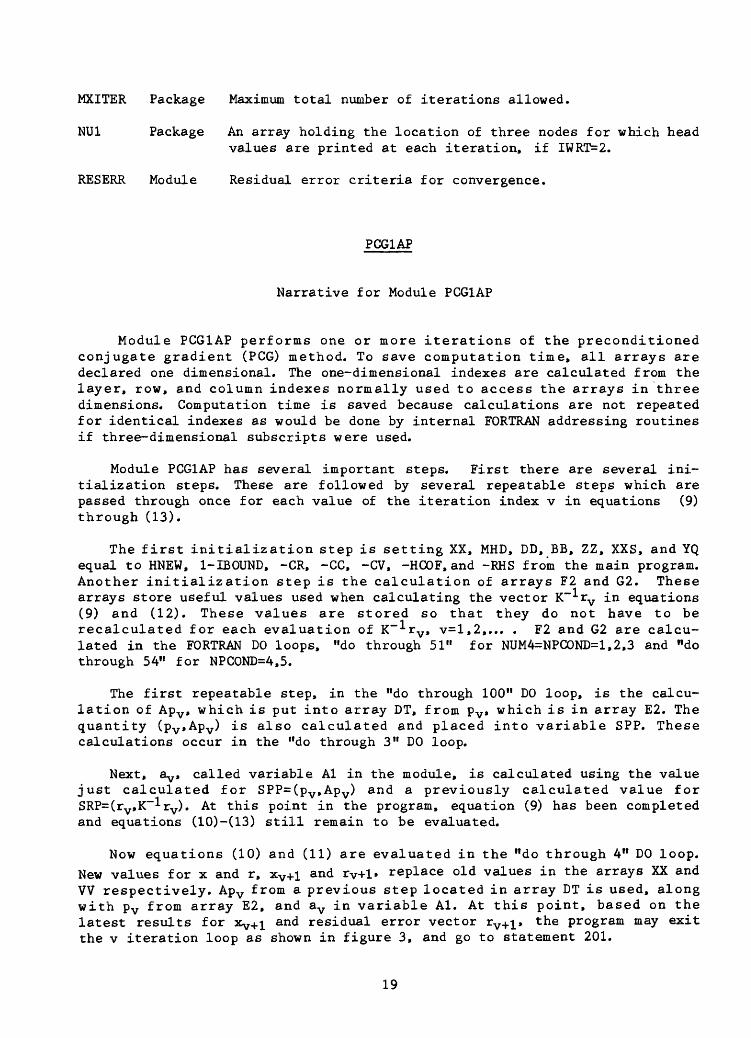
MXITER Package Maximum total number of iterations allowed.
NU1 Package An array holding the location of three nodes for which headvalues are printed at each iteration, if IWRT=2.
RESERR Module Residual error criteria for convergence.
PCG1AP
Narrative for Module PCG1AP
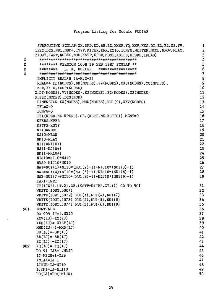
Module PCG1AP performs one or more iterations of the preconditioned conjugate gradient (PCG) method. To save computation time, all arrays are declared one dimensional. The one-dimensional indexes are calculated from the layer, row, and column indexes normally used to access the arrays in three dimensions. Computation time is saved because calculations are not repeated for identical indexes as would be done by internal FORTRAN addressing routines if three-dimensional subscripts were used.
Module PCG1AP has several important steps. First there are several ini tialization steps. These are followed by several repeatable steps which are passed through once for each value of the iteration index v in equations (9) through (13).
The first initialization step is setting XX, MHD, DD, BB, ZZ, XXS, and YQ equal to KNEW, 1-IBOUND, -CR, -CC, -CV, -HCOF, and -RHS from the main program. Another initialization step is the calculation of arrays F2 and G2. These arrays store useful values used when calculating the vector K~^rv in equations (9) and (12). These values are stored so that they do not have to be recalculated for each evaluation of K~^rv, v=l,2,... . F2 and G2 are calcu lated in the FORTRAN DO loops, "do through 51" for NUM4=NPCOND=1,2,3 and "do through 54" for NPCOND=4,5.
The first repeatable step, in the "do through 100" DO loop, is the calcu lation of Apv , which is put into array DT, from pv, which is in array E2. The quantity (pv »Apv) is also calculated and placed into variable SPP. These calculations occur in the "do through 3" DO loop.
Next, av , called variable Al in the module, is calculated using the value just calculated for SPP=(pv,Apv) and a previously calculated value for SRP=(rv,K~^rv). At this point in the program, equation (9) has been completed and equations (10)-(13) still remain to be evaluated.
Now equations (10) and (11) are evaluated in the "do through 4" DO loop. New values for x and r, xv+i and rv+l» replace old values in the arrays XX and VV respectively. Apv from a previous step located in array DT is used, along with pv from array E2, and av in variable Al. At this point, based on the latest results for *v+i and residual error vector rv+i» the program may exit the v iteration loop as shown in figure 3, and go to statement 201.
19
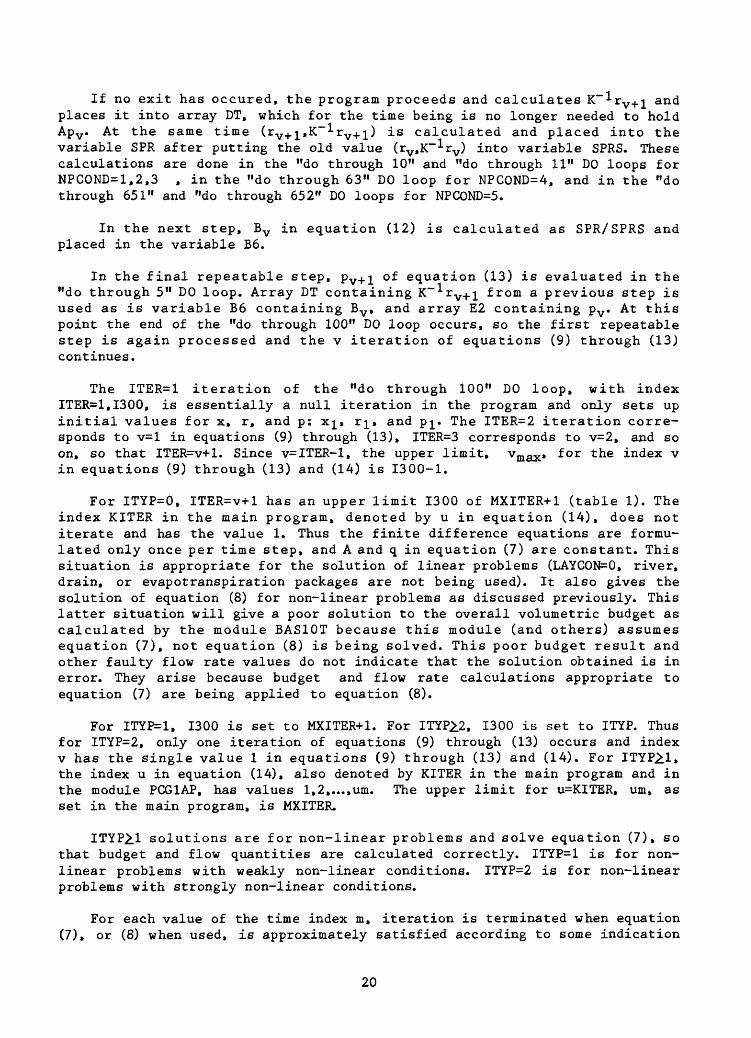
If no exit has occured, the program proceeds and calculates K rv+ i and places it into array DT, which for the time being is no longer needed to hold Apv . At the same time (rv+ i,K~ 1 rv+ i) is calculated and placed into the variable SPR after putting the old value (rv.K~^rv) into variable SPRS. These calculations are done in the "do through 10" and "do through 11" DO loops for NPCOND=1,2,3 , in the "do through 63" DO loop for NPCOND=4, and in the "do through 651" and "do through 652" DO loops for NPCOND=5.
In the next step, Bv in equation (12) is calculated as SPR/SPRS and placed in the variable B6.
In the final repeatable step, pv+i of equation (13) is evaluated in the "do through 5" DO loop. Array DT containing K~-'-rv+ i from a previous step is used as is variable B6 containing Bv , and array E2 containing pv . At this point the end of the "do through 100" DO loop occurs, so the first repeatable step is again processed and the v iteration of equations (9) through (13) continues.
The ITER=1 iteration of the "do through 100" DO loop, with index ITER=1,I300, is essentially a null iteration in the program and only sets up initial values for x, r, and p: x^, rj_, and pj_. The ITER=2 iteration corre sponds to v=l in equations (9) through (13), ITER=3 corresponds to v=2, and so on, so that ITER=v+l. Since v=ITER-l, the upper limit, vmax, for the index v in equations (9) through (13) and (14) is 1300-1.
For ITYP=0, ITER=v+l has an upper limit 1300 of MXITER+1 (table 1). The index KITER in the main program, denoted by u in equation (14), does not iterate and has the value 1. Thus the finite difference equations are formu lated only once per time step, and A and q in equation (7) are constant. This situation is appropriate for the solution of linear problems (LAYCON=0, river, drain, or evapotranspiration packages are not being used). It also gives the solution of equation (8) for non-linear problems as discussed previously. This latter situation will give a poor solution to the overall volumetric budget as calculated by the module BAS10T because this module (and others) assumes equation (7), not equation (8) is being solved. This poor budget result and other faulty flow rate values do not indicate that the solution obtained is in error. They arise because budget and flow rate calculations appropriate to equation (7) are being applied to equation (8).
For ITYP=1, 1300 is set to MXITER+1. For ITYP^.2, 1300 is set to ITYP. Thus for ITYP=2, only one iteration of equations (9) through (13) occurs and index v has the single value 1 in equations (9) through (13) and (14). For ITYP^l, the index u in equation (14), also denoted by KITER in the main program and in the module PCG1AP, has values 1,2,...,urn. The upper limit for u=KITER, urn, as set in the main program, is MXITER.
ITYP^.1 solutions are for non-linear problems and solve equation (7), so that budget and flow quantities are calculated correctly. ITYP=1 is for non linear problems with weakly non-linear conditions. ITYP=2 is for non-linear problems with strongly non-linear conditions.
For each value of the time index m, iteration is terminated when equation (7), or (8) when used, is approximately satisfied according to some indication
20
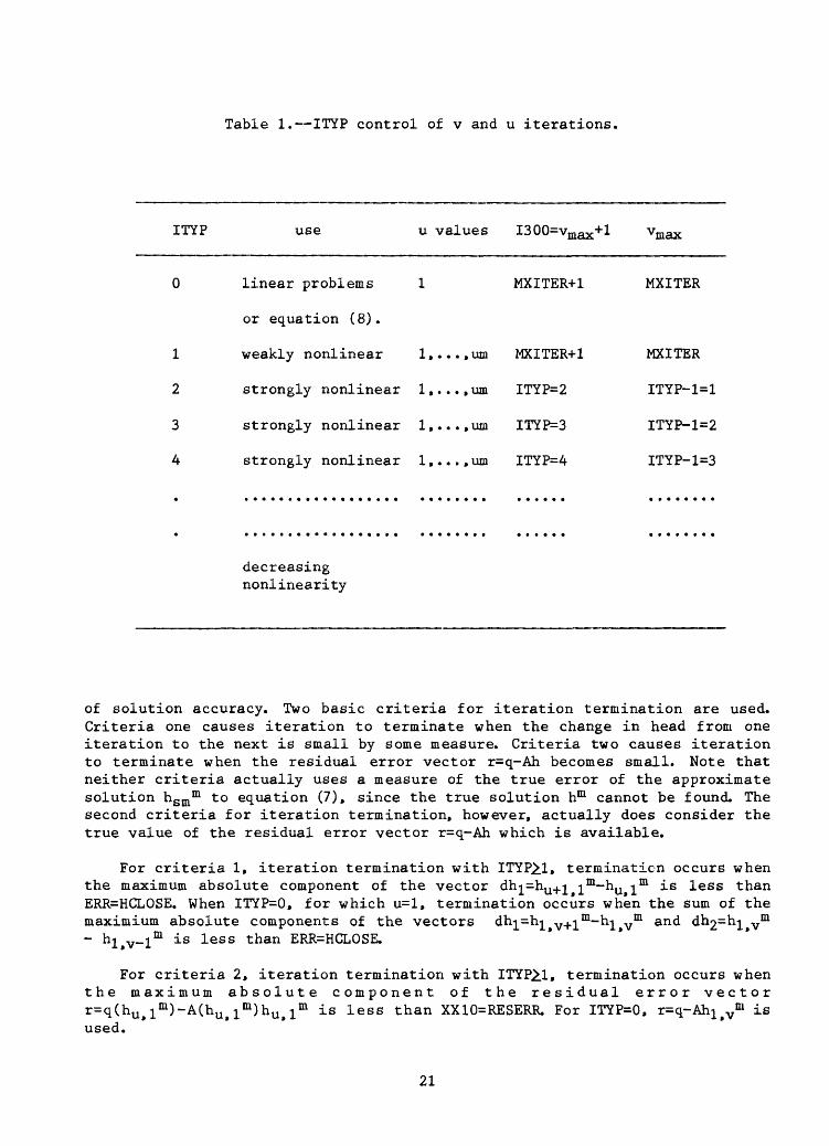
Table 1. ITYP control of v and u iterations.
ITYP use u values I300=vmax+l 'max
0
1
2
3
4
linear problems
or equation (8) .
weakly nonlinear
strongly nonlinear
strongly nonlinear
strongly nonlinear
1
1, . . . ,um
1 , . . . , um
1, . . . ,um
MXITER+1
MXITER+1
ITYP=2
ITYP=3
ITYP=4
MXITER
MXITER
ITYP-1=1
ITYP-1=2
ITYP 1~3
decreasing nonlinearity
of solution accuracy. Two basic criteria for iteration termination are used. Criteria one causes iteration to terminate when the change in head from one iteration to the next is small by some measure. Criteria two causes iteration to terminate when the residual error vector r=q-Ah becomes small. Note that neither criteria actually uses a measure of the true error of the approximate solution hsmm to equation (7), since the true solution hm cannot be found. The second criteria for iteration termination, however, actually does consider the true value of the residual error vector r=q-Ah which is available.
For criteria 1, iteration termination with ITYP^.1, termination occurs when the maximum absolute component of the vector dh^=hu+^ l m~nu i m ^ s less than ERR=HCLOSE. When ITYP=0, for which u=l, termination occurs when the sum of themaximium absolute components of the vectors dh^=h^ - h- m is less than ERR=HCLOSE.
vm an<^ vm
For criteria 2, iteration termination with ITYP2.1, termination occurs when the maximum absolute component of the residual error vector r=q(hu>1 m )-A(hu>1 m)hu>1 m is less than XX10=RESERR. For ITYP=0, r=q-Ah1>vm is used.
21
Flow Chart
for
Module PCG1AP
ro
ro
RENT
ER P
CG
IAPJ
^ rS
ET
IC
NV
G=0
. F
NE
W T
ME
ST
EP
. S
ET
MC
NT
-0.
SE
T A
RR
AY
S X
X.
MH
D.
DD
. B
B.
ZZ
. X
XS
. A
ND
YQ
. E
QU
AC
TO
HN
EW
. 1H
BO
UN
D,
-CR
. -C
C.
-CV
. -H
CO
F.
AN
D
-RH
S F
RO
M T
HE
MA
IN
PR
OG
RA
M.
CA
LC
UL
AT
E A
RR
AY
S
F2
AN
D G
2.
SE
T I
FLA
G=
0.
1f
SE
T I
300=
MX
ITE
R+
1
FO
R
ITY
P=
0.1.
S
ET
13
00 I
TY
P F
OR
IT
YP
i2.
1r
SE
T I
TE
R=0
1r
SE
T
ITE
R=I
TE
R+1
A
ND
MC
NT
=M
CN
T+
1 .
CA
LC
ULA
TE
A1.
XX
, A
ND
VV
U
SIN
G
EQ
UA
TIO
NS
(9
) -
(11).
WH
ER
E I
TE
R=
v+1.
F
OR
IW
RT
=2,
PR
INT
OU
T C
ON
VE
RG
EN
CE
WA
TC
HIN
G O
UT
PU
T.
Vr
/
(ER
5+E
R5S
)< E
RR
? \
YE
SV
S
RZ
<X
X10
?
/
NO
^
( M
CN
T^M
NO
1
r vM
-rrr
r>
n \ ' "-
^
r|
CA
LC
UL
AT
E
E2
US
ING
EQ
UA
TIO
NS
C12
) -
C13
).
|
r i i
rj° /
\4
-1
f F
OR
IT
YP
=0
\ - t /
SE
T
ICN
VG
=1
./O
R
ITY
\
MC
NT
>
NO
^P=0
\
YE
S
MX
ITE
R ?
/
4
c
f
CA
LC
UL
AT
E D
XM
AX
|
1r
1 r
>ET
IFLA
G=1
/
ITY
P >
1
AN
D C
DX
MA
X <
ER
R \
YE
SY
O
R S
RZ
1^X
X10)
? /
NO
iY
ES
/
ICN
VG
=
\
IFLA
(
NO
i
r 0 A
ND
\
3*1
/
t
PR
INT
M
CN
T.
KS
TP
. K
PE
R
|
ir
FO
R IW
RT
^I,
PR
INT
ER
5 A
ND
: S
RZ
A
ND
SU
MR
Z F
OR
IT
YP
=0,
OR
SR
Z1
AN
D S
UM
RZ
1 F
OR
IT
YP
> 0
.
*t
C
RE
TU
RN
J
1E
T IC
NV
G=1
|
Program Listing for Module PCG1AP
SUBROUTINE PCG1AP(XX,MHD,DD,BB,ZZ,XXSP,YQ,XXV,XXS,DT,E2,F2,G2,W, 1lE22,D2S,NUl,NUM4,ITYP,KITER,ERR,XX10,ICNVG,MXITER,NCOL,NROW,NLAYf 22IOUT,IWRT,NODES,NOD,KSTP.KPER.MCNT.KSTPS.KPERS,IFLAG) 3
C ******************************************* 4C ******** VERSION 1008 19 FEB 1987 PCG1AP ** 5C ******** L. K. KUIPER ***************** 6C ******************************************* 7
IMPLICIT REAL*8 (A-H.O-Z) 8REAL*4 DD(NODES),BB(NODES),ZZ(NODES),XXS(NODES),YQ(NODES), 91ERR,XX10,XXSP(NODES) 102.DT(NODES),W(NODES),E2(NODES),F2(NODES),G2(NODES) 113.E22(NODES),D2S(NOD) 12
DIMENSION XX(NODES),MHD(NODES),NU1(9),XXV(NODES) 13IFLAG=0 14ICNVG=0 15IF((KPER.NE.KPERS).OR.(KSTP.NE.KSTPS)) MCNT=0 16KPERS=KPER 17KSTPS=KSTP 18NI10=NCOL 19NJ10=NROW 20NK10=NLAY 21NI11=NI10+1 22NJ11=NJ10+1 23NK11=NK10+1 24NIJ10=NI10*NJ10 25N320=NLJ10*NK10 26NW1=NU1(1)+NI10*(NU1(2)-1)+NIJ10*(NU1(3)-1) 27NW2=NU1(4)+NI10*(NU1(5)-1)+NIJ10*(NU1(6)-1) 28NW3=NU1(7)+NI10*(NU1(8)-1)+NIJ10*(NU1(9)-1) 29 IWR1+IWRTIF((IWR1.LT.2).OR.(KSTP*KITER.GT.1)) GO TO 901 31WRITE(IOUT,5007) 32WRITE(IOUT,5072) NU1(1),NU1(4),NU1(7) 33WRITE(IOUT,5073) NU1(2),NU1(5),NU1(8) 34WRITE(IOUT,5074) NU1(3),NU1(6),NU1(9) 35
901 CONTINUE 36DO 909 IJ=1,N320 37XXV(IJ)=XX(IJ) 38XXS(IJ)=-XXSP(IJ) 39MHD(IJ)=1-MHD(IJ) 40DD(IJ)=-DD(IJ) 41BB(IJ)=-BB(IJ) 42ZZ(IJ)=-ZZ(IJ) 43
909 YQ(IJ)=-YQ(IJ) 44DO 91 IJB=1,N320 45IJ=N320+1-IJB 46IM1JK=IJ-1 47IJM1K=IJ-NI10 48IJKM1=IJ-NIJ10 49DD(IJ)=DD(IM1JK) 50
23
BB(IJ)=BB(IJM1K) 51ZZ(IJ)=ZZ(IJKM1) 52
91 CONTINUE 53DO 92 K=1.NK10 54DO 92 J=1.NJ10 55DO 92 I=1.NI10 56 IJ=I+NI10*(J-D+NIJ10*(K-1) 57IF(I.EQ.l) DD(IJ)=0 58IF(J.EQ.l) BB(IJ)=0 59IF(K.EQ.l) ZZ(IJ)=0 60
92 CONTINUE 61DO 1 IJ=1,N320 62DT(IJ)=0 63E2(IJ)=0 64F2(IJ)=0 65G2(IJ)=0 66E22(IJ)=0 67
1 W(IJ)=0 68NN=NROW+NCOL 69DO 2 IJ=1.NN 70
2 D2S(IJ)=0 71DO 16 IJ=1,N320 72E2(IJ)=XX(IJ) 73 IF(MHD(IJ).GE.l) GO TO 16 74W(IJ)=YQ(IJ) 75
16 CONTINUE 76 IF(NUM4.GE.4) GO TO 74 77
71 CONTINUE 78Yl=0 79Zl=0 80DO 51 IJ=1,N320 81 IF(.NOT.(MHD(IJ).GE.l)) GO TO 777 82Yl=0 83Zl=0 84D2S(NI10+1)=0 85DO 94 I=1.NI10 86
94 D2S(I)=D2S(I+1) 87GO TO 51 88
777 CONTINUE 89IM1JK=IJ-1 90IJM1K=IJ-NI10 91IJKM1=IJ-NIJ10 92IDM=1 93IBM=1 94IZM=1 95IF(IMUK.LT.l) IDM=0 96IF(IJMlK.LT.l) IBM=0 97IF(IJKMl.LT.l) IZM=0 98IP1JK=IJ+1 99IJP1K=IJ+NI10 100IJKP1=IJ+NIJ10 101IDP=1 102IBP=1 103
24
IZP=1 104 IF(IP1JK.GT.N320) IDP=0 . 105IF(IJP1K.GT.N320) IBP=0 106IF(IJKP1.GT.N320) IZP=0 107X=DD(IJ) 108Y=BB(IJ) 109Z=ZZ(IJ) 110 EEIJ=-(X+Y+Z+IDP*DD(IP1JK) +IBP*BB(IJP1K)+IZP*ZZ(IJKPl))+XXS(IJ) 111 IF(MHD(IMUK)*IDM.GE.l) X=0 112 IF(MHD(IJM1K)*IBM.GE 1) Y=0 113 IF(MHD(IJKMl)*IZM.GE.l) Z=0 114Y1Z1=0 115XP=X 116YP=Y 117F2X=F2(IM1JK)*IDM 118F2Y=F2(IJM1K)*IBM 119F2Z=F2(IJKM1)*IZM 120IF(NUM4.EQ.l) GO TO 20 121JP1=IJ-NI10+1 122KP1=IJ-NIJ10+1 123IJMMN=IJ-(NIJ10-NI10) 124UP1=1 125IKP1=1 126IMMN=1 127IF(JPl.LT.l) IJP1=0 128IF(KPl.LT.l) IKP1=0 129IF(IJMMN.LT.l) IMMN=0 130WY1=0 131WZ1=0 132 IF(F2Y.NE.O.O) WY1=Y/F2Y 133 IF(F2Z.NE.O.O) WZ1=Z/F2Z 134XP=X-(WY1*Y1+WZ1*Z1) 135G2(IJ)=XP 136YP=Y-WZ1*D2S(1) 137E22(IJ)=YP 138Y1=-WY1*G2(JP1)*IJP1 139Z1=-WZ1*G2(KP1)*IKP1 140ZB=-WZ1*E22(IJMMN)*IMMN 141D2S(NI10+1)=ZB 142DO 93 I=1.NI10 143
93 D2S(I)=D2S(I+1) 144F21=F2(JP1)*IJP1 145F22=F2(KP1)*IKP1 146F23=F2(IJMMN)*IMMN 147Pl=0 148P2=0 149P3=0 150 IF(F21.NE.O.O) P1=Y1*Y1/F21 151 IF(F22.NE.O.O) P2=Z1*Z1/F22 152 IF(F23.NE.O.O) P3=ZB*ZB/F23 153Y1Z1=P1+P2+P3 154
20 CONTINUE 155XF=0 156
25
YF=0 157ZF=0 158IF(F2X.NE.O.O) XF=XP*XP/F2X 159IF(F2Y.NE.O.O) YF=YP*YP/F2Y 160IF(F2Z.NE.O.O) ZF=Z*Z/F2Z 161F2dJ)=EEIJ-(XF+YF+ZF+YlZl) 162
51 CONTINUE 163GO TO 80 164
74 CONTINUE 165DO 54 IJ=1.N320 166IF(MHD(IJ).GE.l) GO TO 54 167IP1JK=IJ+1 168IJP1K=IJ+NI10 169IJKP1=IJ+NIJ10 170IDP=1 171IBP=1 172IZP=1 173IFUP1JK.GT.N320) IDP=0 174IFCUP1K.GT.N320) IBP=0 175IF(IJKP1.GT.N320) IZP=0 176 EEIJ= (-(DDdJ)+BBdJ)+ZZdJ)+IDP*DDdPUK) 177
!+IBP*BBdJPlK)+IZP*ZZdJKPl))+XXSdJ)) 178IF(NUM4.EQ.4) GO TO 539 179X=DD(IJ) 180F2X=F2(IJ-1) 181XF=0 182IF(F2X.NE.O.O) XF=X*X/F2X 183F2(IJ)=EEIJ-XF 184GO TO 54 185
539 F2(IJ)=EEIJ 18654 CONTINUE 18780 CONTINUE 188
SPR=1.D-50 189ICNT=-1 190ER5S=1.D40 191I300=MXITER+1 192IFdTYP.GE.2) I300=ITYP 193DO 100 ITER=1.I300 194ICNT=ICNT+1 195 IF(ITER*KITER*KSTP*KPER.EQ.l) MCNT=0 196IF(ITER.NE.l) MCNT=MCNT+1 197SPP=0 198DO 3 IJ=1.N320 199IF(MHD(IJ).GE.l) GO TO 3 200IP1JK=IJ+1 201IJP1K=IJ+NI10 202IJKP1=IJ+NIJ10 203IDP=1 204IBP=1 205IZP=1 206IF(IP1JK.GT.N320) IDP=0 207IF(IJP1K.GT.N320) IBP=0 208IF(IJKP1.GT.N320) IZP=0 209
26
IJM1K=IJ-NI10 210LJKM1=IJ-NIJ10 211DDIJ=DD(IJ) 212DDIP1=DD(IP1JK)*IDP 213BBIJ=BB(IJ) 214BBIJP=BB(IJP1K)*IBP 215ZZIJ=ZZ(IJ) 216ZZIJK=ZZ(IJKPl)*IZP 217E2IJ=E2(IJ) 218 DTIJ=(-(DDIJ+DDIP1+BBIJ+BBIJP+ZZIJ+ZZIJK)+XXS(IJ))*E2IJ 219 1+DDIJ*E2( IJ-1)+DDIP1*E2(IP1JK) 220 2+BBIJ*E2(IJMlK)+BBIJP*E2(IJPlK) 221 3+ZZIJ*E2(IJKMl)+ZZIJK*E2(IJKPl) 222DT(IJ)=DTIJ 223SPP=SPP+E2IJ*DTLJ 224
3 CONTINUE 225A1=SPR/(SPP+1.D-50) 226A2=A1 227IF(ITER.GT.l) GO TO 35 228Al=0 229A2=l. 230
35 SRZ=0 231SUMRZ=0 232ER5=0 233DO 4 K=1,NK10 234DO 4 J=1,NJ10 235DO 4 I=1,NI10 236 IJ=I+NI10*(J-1)+NIJ10*(K-1) 237IF(MHD(IJ).GE.l) GO TO 4 238DX=A1*E2(IJ) 239IF(MHD(IJ).EQ.2) DX=0 240X=XX(IJ)+DX 241XX(IJ)=X 242ADX=DABS(DX) 243IF(ADX.LT.ERS) GO TO 111 244IMX=I 245JMX=J 246KMX=K 247XXPMX=X 248ER5=ADX 249
111 CONTINUE 250X=W(IJ)-A2*DT(IJ) 251SUMRZ=SUMRZ+X 252DSR=DABS(X) 253IF(DSR.GT.SRZ) SRZ=DSR 254W(IJ)=X 255
4 CONTINUE 256IF(ITER.EQ.l) SRZ1=SRZ 257IF(ITER.EQ.l) SUMRZ1=SUMRZ 258 IF((IWRl.GE.2).AND.(ITER.NE.l)) WRITE(IOUT.1000) MCNT.ICNT, IMX. 259
1JMX.KMX,XXPMX,ER5,SRZ,XX(NW1).XX(NW2).XX(NW3) 260X5=.5 261IF(ITER.LE.2) X5=1.0 262
27
IF(((ER5+ER5S)*X5).LT.ERR) GO TO 201 263IF(SRZ.LT.XXIO) GO TO 201 264 IF(MCNT.EQ.MXITER) GO TO 202 265ER5S=ER5 266SPRS=SPR 267SPR=0 268 GOTO (81,81.81,83,85),NUM4 269
81 CONTINUE 270DO 10 IJ=1,N320 271IF(MHD(IJ).GE.l) GO TO 10 272IJM1K=IJ-NI10 273IJKM1=IJ-NIJ10 274B6=0 275Z6=0 276DDIJ=DD(IJ) 277BBIJ=BB(IJ) 278IF(NUM4.EQ.l) GO TO 21 279DDIJ=G2(IJ) 280BBIJ=E22(IJ) 281JP1=IJ-NI10+1 282KP1=IJ-NIJ10+1 283IJMMN=IJ-(NIJ10-NI10) 284B6=0 285Z6=0 286F2J=F2(IJM1K) 287F2K=F2(IJKM1) 288 IF(F2J.NE.O.DO) B6=DT(JP1)*G2(JP1)/F2J 289 IF(F2K.NE.O.DO) Z6=(DT(KP1)*G2(KP1)+DT(IJMMN)*E22(IJMMN))/F2K 290
21 CONTINUE 291DT(IJ) = (W(IJ)-DDIJ*DT(IJ-1)-BBIJ*(DT(IJM1K)-B6) 2921-ZZ(IJ)*(DT(IJKM1)-Z6))/F2(IJ) 293
10 CONTINUE 294DO 11 IJB=1,N320 295IJ=N320+1-IJB 296IF(MHD(IJ).GE.l) GO TO 11 297IP1JK=IJ+1 298IJP1K=IJ+NI10 299IJKP1=IJ+NIJ10 300IDP=1 301IBP=1 302IZP=1 303IF(IP1JK.GT.N320) IDP=0 304IF(IJP1K.GT.N320) IBP=0 305IF(IJKP1.GT.N320) IZP=0 306XAD=0 307DDD=DD(IP1JK) 308BBB=BB(IJP1K) 309IF(NUMA.EQ.l) GO TO 22 310JM1=U+NI10-1 311KM1=IJ+NIJ10-1 312IJPMN=IJ+(NIJ10-NI10) 313IJM1=1 314IKM1=1 315
28
IPMN=1 316IF(JM1.GT.N320) UM1=0 317IF(KM1.GT.N320) IKM1=0 318IF(IJPMN.GT.N320) IPMN=0 319IM1JK=IJ-1 320UM1K=IJ-NI10 321IDM=1 322IBM=1 323IF(IMUK.LT.l) IDM=0 324IF(UMlK.LT.l) IBM=0 325DDD=G2(IPIJK) 326BBB=E22(IJPIK) 327XAD1=0 328XAD2=0 329F2I=F2(IM1JK)*IDM 330F2J=F2(IJM1K)*IBM 331 IF(F2I.NE.O.DO) XAD1=-(E22(JM1)*IJM1*DT(JM1)+ZZ(KM1)*IKM1* 332
1DT(KM1))*G2(IJ)/F2I 333 IF(F2J.NE.O.DO) XAD2=-ZZ(IJPMN)*IPMN*E22(IJ)*DT(IJPMN)/F2J 334XAD=XAD1+XAD2 335
22 CONTINUE 336DTIJ=DT(IJ)-(DDD*IDP*DT(IPIJK)+BBB*IBP*DT(IJPIK)+ZZ(IJKPl) 337
1*IZP*DT(IJKPl)+XAD)/F2(IJ) 338DT(IJ)=DTIJ 339SPR=SPR+DTU*W(IJ) 340
11 CONTINUE 341GO TO 90 342
83 CONTINUE 343DO 63 IJ=1,N320 344IF(MHD(IJ).GE.l) GO TO 63 345F2IJ=F2(IJ) 346WIJ=W(IJ) 347DTIJ=WIJ/F2IJ 348DT(IJ)=DTIJ 349SPR=SPR+DTIJ*WIJ 350
63 CONTINUE 351GO TO 90 352
85 CONTINUE 353DO 651 IJ=1,N320 354IF(MHD(IJ).GE.l) GO TO 651 355 DT(IJ) = (W(IJ)-DD(IJ)*DT(IJ-1))/F2(IJ) 356
651 CONTINUE 357DO 652 IJB=1,N320 358IJ=N320+1-IJB 359IF(MHD(IJ).GE.l) GO TO 652 360IP1JK=IJ+1 361 DTIJ=DT(IJ)-DD(IP1JK)*DT(IP1JK)/F2(IJ) 362DT(IJ)=DTIJ 363SPR=SPR+DTU*WdJ) 364
652 CONTINUE 36590 CONTINUE 366
B6=SPR/SPRS 367IF(ITER.EQ.l) B6=0 368
29
DO 5 IJ=1,N320 369E2IJ=DT(IJ)+B6*E2(IJ) 370IF(MHD(IJ).GE.l) E2IJ=0 371E2(IJ)=E2IJ 372
5 CONTINUE 373100 CONTINUE 374
GO TO 202 375201 IF(ITYP.EQ.O) ICNVG=1 376202 CONTINUE 377
IF((MCNT.GE.MXITER).OR.(ITYP.EQ.O)) IFLAG=1 378DXMAX=0 379DO 19 IJ=1,N320 380XXVIJ=XXV(IJ) 381DX=DABS(XX(IJ)-XXVIJ) 382IF(DX.GT.DXMAX) DXMAX=DX 383IP1JK=IJ+1 384IJP1K=IJ+NI10 385IJKP1=IJ+NIJ10 386DD(IJ)=DD(IP1JK) 387BB(IJ)=BB(LJP1K) 388ZZ(IJ)=ZZ(IJKP1) 389
19 CONTINUE 390 IF((ITYP.GE.l).AND.((DXMAX.LE.ERR).OR.(SRZI.LT.XXIO))) ICNVG=1 391DO 919 IJ=1,N320 392MHD(IJ)=1-MHD(IJ) 393DD(IJ)=-DD(IJ) 394BB(IJ)=-BB(IJ) 395ZZ(IJ)=-ZZ(IJ) 396
919 YQ(IJ)=-YQ(IJ) 397DO 991 IJ=1,N320 398
991 XXSP(IJ)=-XXS(IJ) 399IF((ICNVG.EQ.O).AND.(IFLAG.NE.l)) GO TO 600 400IF(KSTP.EQ.l) WRITE(IOUT,500) 401S1=SRZ 402S2=SUMRZ 403IF(ITYP.EQ.O) GO TO 518 404S1=SRZ1 405S2=SUMRZ1 406
518 CONTINUE 407WRITE(IOUT,501) MCNT.KSTP.KPER 408IF(IWRT.GE.l) WRITE(IOUT,5075) ER5.S1.S2 409
500 FORMAT(1HO) 410501 FORMAT(IX,15,' ITERATIONS FOR TIME STEP 1 ,14,' IN STRESS PERIOD 1 , 411
113) 4121000 FORMAT(' ',2I3,3I4,6D18.7) 4135007 FORMAT('0',56X,'WATCHING CONVERGENCE'//25X.'THE MAXIMUM CHANGE IN 414
1HEAD OCCURED AT COLUMN J, ROW I, LAYER K.' 4152 /25X,'MAXIMUM RESIDU 4163AL ERROR = THE MAXIMUM OVER ALL THE GRID ELEMENTS OF THE'/25X,»DI 4174FFERENCE BETWEEN THE WATER FLOW RATE INTO AND OUT OF EACH GRID ELE 4185MENT.') 419
5074 FORMAT(7X,' J I K',5X,'HEAD AT J.I.K',5X,'HEAD AT J.I.K',13X 4201,'ERROR',3(12X,»K=',I4)) 421
30
5072 FORMAT('0'.72X.3(4X.'HEAD AT J='.I4)) 4225073 FORMAT(46X.'CHANGE IN'.6X.'MAX RESIDUAL 1 .3(12X.'!='.14)) 4235075 FORMAT( 424
I'O'.'MAXIMUM CHANGE IN HEAD BETWEEN LAST 2 ITERATIONS ='.D11.3/ 4252' MAXIMUM RESIDUAL ERROR (L**3/T) FOR GRID ELEMENTS NOT HAVING FIX 4263ED HYDRAULIC HEAD ='.D11.3.' TOTAL ='.D11.3) 427
600 RETURN 428END 429
List of Variables for Module PCG1AP
Variable Range
Al Module
B6 Module
BB Module
DD Module
DT Module
DXMAX Module
E2 Module
ER5 Module
ER5S
ERR
F2
G2
1300
ICNVG
IFLAG
Module
Module
Module
Module
Module
Global
Global
Definition
ay in equation (9) .
Bv in equation (12) .
-B in equation (2) .
-D in equation (2) .
Work space array used when calculating equations (9) through (13).
for criteria 1 ITYP^.1 iteration termination.
Vector pv in equations (9) through (13) .
for criteria 1 ITYP=0 iteration termination. Called maximum absolute head change when printed out.
for criteria 1 ITYP=0 iteration termination.
HCLOSE in module PCG1RP. The head change criteria for convergence.
Storage array used when calculating K~^-rv in equations (9) and (12).
Same as above.
Maximum value for iteration counter ITER. Equal to vmax+l of figure 3.
This flag is set to one when iteration has met the condi tions for iteration termination.
This flag is set to one when exit is desired from the u iteration loop in the main program, due either to MCNT^MXITER or ITYP=0.
31
IOUT Global Primary unit number for all printed output. IOUT=6.
ITER Module Iteration counter for v in equations (9) through (13),ITER=v+l.
Flag indicating the type of problem being solved.
Flag indicating the amount of output desired.
Iteration counter u in equation (14). Reset at the start of each time step.
Stress period counter.
Stored value of KPER.
Time step counter. Reset at the start of each stress period.
Stored value of KSTP.
Iteration number counter that counts the total number of iterations that are used as indices u and v increase in equations (9) through (13) and (14).
An array to indicate when a node is active and if it has a fixed head. MHD is equal to 1-IBOUND from the main program.
Maximum total number of iterations allowed.
Number of columns in the grid.
Number of layers in the grid.
Number of cells (nodes) in the finite difference grid.
Number of rows in the grid.
An array holding the location of three nodes for which head values are printed at each iteration, if IWRT=2.
NUM4 Module Called NPCOND in module PCG1AL. Has values of 1 to 5 forthe 5 preconditioning types.
SRZ Module Maximum absolute component of the residual error vector rfor ITYP=0 criteria 2 iteration termination. Called maxi mum absolute residual error when printed out.
SRZ1 Module Maximum absolute component of the residual error vector rfor ITYP^.1 criteria 2 iteration termination. Called maxi mum absolute residual error when printed out.
ITYP
IWRT
KITER
KPER
KPERS
KSTP
KSTPS
MCNT
MHD
MXITER
NCOL
NLAY
NODES
NROW
NU1
Package
Package
Global
Global
Module
Global
Module
Module
Module
Package
Global
Global
Global
Global
Package
32
SUMRZ Module Total residual error, ITYP=0.
SUMRZ1 Module Total residual error, ITYP^l.
W Module Error vector rv in equations (9) through (13).
XX10 Module Called RESERR in module PCG1RP. The residual errorcriteria for convergence.
XX Module Head vector h. Vector xv in equations (9) through (13).KNEW in the main program.
XXS Module -HCOF in equation (1).
XXV Module Stored XX array. Used to get DXMAX.
YQ Module -RHS in equation (1).
ZZ Module -Z in equation (2).
33
REFERENCES
Hageman, L. A., and Young, D. M., 1981, Applied Iterative Methods, New York, Academic Press, 386 p.
Kershaw, D. S., 1978, The incomplete Choleski-conjugate gradient method for the iterative solution of linear equations: Journal of Computational Physics, v. 26, p. 43-65.
Kuiper, L. K., 1981, A comparision of the incomplete Choleski-conjugate gradient method with the strongly implicit method as applied to the solution of two-dimensional groundwater flow equations: Water Resources Research, v. 17, no. 4, p. 1082.
Kuiper, L. K., 1987, A comparison of iterative methods as applied to the solution of the nonlinear three-dimensional groundwater flow equation: Society for Industrial and Applied Mathematics Journal on Scientific and Statistical Computing, v. 8, no. 4, p. 521-528.
McDonald, M. G., and Harbaugh, A. W., 1984, A modular three-dimensional finite difference ground-water flow model: U.S. Geological Survey Open-File Report 83-875, 528 p.
Van Der Vorst, H. A., 1982, A vectorizable variant of some ICCG methods: Society for Industrial and Applied Mathematics Journal on Scientific and Statistical Computing, v. 3, no. 3, p. 350-356.
34