580 | Soft Matter, 2021, 17, 580--591 This journal is©The Royal Society of Chemistry 2021

Cite this: SoftMatter, 2021,

17, 580

Computer modeling of polymer stars in variablesolvent conditions: a comparison of MDsimulations, self-consistent field (SCF) modelingand novel hybrid Monte Carlo SCF approach

Alexander D. Kazakov, *a Varvara M. Prokacheva, a Filip Uhlık,a

Peter Kosovan a and Frans A. M. Leermakers b

Computer-aided modeling is a systematic approach to grasp the physics of macromolecules, but it

remains essential to know when to trust the results and when not. For a polymer star, we consider three

approaches: (i) Molecular Dynamics (MD) simulations and implementing a coarse-grained model, (ii) the

self-consistent field approach based on a mean-field approximation and implementing the lattice model

due to Scheutjens and Fleer (SF-SCF) and (iii) novel hybrid Monte Carlo self-consistent field (MC-SCF)

method, which combines a coarse-grained model driven by a Monte Carlo method and a mean-field

representation driven by SF-SCF. We compare the performance of these approaches under a wide range

of solvent qualities. The MD approach is formally the most exact but suffers from reasonable

convergence. The mean-field approach works similarly in all solvent qualities but is quantitatively least

accurate. The MC-SCF hybrid allows us to combine the benefits of the simulation route and the

effective performance of SCF. We consider the center-to-end distance Rce, the radius of gyration Rg2 of

the star and the polymer density profiles j(r) of polymer-segments in it. All three methods show a good

qualitative agreement one to another. The MC-SCF method is in good agreement with the scaling

predictions in the whole range of solvent quality values showing that it grasps the essential physics while

remaining computationally in bounds.

1 Introduction

The polymer coil is one of the most soft objects known to man.Its softness, but also many other properties, continues tofascinate scientists across disciplines. There are various waysone can get deeper insight in its intricate behaviors. Computeraided modeling is a prominent tool that is frequently usedfor this. There are various methods all with their own prosand cons.

Computer simulations, for example, are used to predicteffects such as the swelling or compression of coils, somethingthat might be hard and/or expensive to lay your hand on usingexperiments. Simulations might also be used to deepen ourknowledge in general.1 With computer simulations, one typicallysamples phase space and by doing so one builds up knowledge ofthe (exact) system partition function. In turn, this function holds

all insights that we can know about the system of interest.Their predictions are valuable and undeniably contribute toour knowledge. With the increasing strength of computerresources the computer simulation tool gains in importance.

In many cases, however, computer simulations do not (yet)resolve all issues. In particular, there may be length- and timescale challenges in combination with limited computationalresources that prevent us from reaching acceptably small valuesfor the statistical error estimation of targeted measurables.When this happens, one may even argue that it is meaninglessto discuss values for the targeted effects, or one may even doubtwhether simulations can relate to the existence per se of thetargeted effect.

In cases when simulation methods are in trouble, that isin particular when satisfactory statistical accuracies cannotbe reached, we may resort to alternatives. Invariably, these arebased upon mean-field approximations and focus on the mean-field partition function. These approximations are implementedspecifically to reduce the computation time and because in somecases, one can even make progress analytically. The mean-fieldapproximation is a good example of sacrificing the systemresolution to reach effective probability distributions.

a Department of Physical and Macromolecular Chemistry, Faculty of Science,

Charles University, Hlavova 8, 128 00 Praha 2, Czech Republic.

E-mail: aleksandr.kazakov@natur.cuni.czb Department of Agrotechnology and Food Sciences, Wageningen University and

Research Center, Wageningen, The Netherlands

Received 11th June 2020,Accepted 28th October 2020

DOI: 10.1039/d0sm01080d

rsc.li/soft-matter-journal

Soft Matter

PAPER

Publ

ishe

d on

29

Oct

ober

202

0. D

ownl

oade

d by

UN

IVE

RSI

TY

OF

CIN

CIN

NA

TI

on 3

/11/

2021

2:4

0:10

PM

.

View Article OnlineView Journal | View Issue

This journal is©The Royal Society of Chemistry 2021 Soft Matter, 2021, 17, 580--591 | 581

One prominent simulation method that gains importance,and is used below, is Molecular Dynamics (MD) simulations.MD samples the partition function by integrating the Newtonlaw of motion. It accounts for correlations between segmentinteractions and therefore the method earned well-deservedrecognition in the scientific audience and hence in the com-munity of modeling of macromolecules. However, with anincreasing number of segments in a polymer chain, MD simu-lation becomes less efficient and suffers from slow dynamicsand accumulated errors.2,3 For long polymer chains, we have tosacrifice the resolution of a system to get statistically reliableresults. The MD technique is also limited because it has justone strategy to sample the degrees of freedom. When thedynamics is not per se of interest and the sampling of onlythe equilibrium properties is targeted, one can alternatively usethe Monte Carlo (MC) simulation method. This method is anensemble sampling approach that can make use of arbitrarychanges of the system degrees of freedom and not necessarily onesthat pass by through the motion of the molecule. By inventingarbitrary moves such that all phase space variables (typically thepositional coordinates of all particles) can be reached, one canmore effectively than MD, sample the Boltzmann distribution thatcharacterizes equilibrium. MC can be used with exactly the samemolecular model as MD and typically employs the Metropolisalgorithm to guarantee that the Boltzmann distribution is indeedobserved. When MD has trouble reaching the equilibrium distribu-tion, also MC will quickly be in trouble. Hence the two methods arereally complementary to each other but are limited in practice to’small systems’.2 MD may be preferred in cases when the coil isdense, while MC may be preferred for more open coils dependingon the success of the sampling techniques. When the samplingis sufficiently rigorous both methods give the same exact results(for the same model).

The self-consistent field approach for inhomogeneouspolymer systems using the Scheutjens–Fleer protocol (SF-SCF)is our mean-field approach that is embraced. This techniquewill not give the rigorous result, but an approximate one andalso the model that is implemented has adjusted characteristics.In SF-SCF, one does not determine individual segmentconfigurations, instead one evaluates their overall distributionsbased on the interactions of the segments with their averagedenvironment. This makes the method faster because, unlike inMD or MC, one averages over all chain configurations at once.This goes at the cost of neglecting some correlation and themethod must of course be validated for each task that it isused for.

In this paper, we not only make use of the MD and theSF-SCF route, but specifically we elaborate on a hybrid methodthat combines the MC approach with the SF-SCF method suchthat we take advantage of the benefits of both methods. We willrefer to this as the MC-SCF hybrid. In short, part of the degreesof freedom (segments) for the polymer coil will be managedby MC (so-called explicit segments). The remainder of thesegments is handled by SF-SCF (so-called implicit segments).Importantly, the number of segments that is accounted forexplicitly may be tuned and therefore we can go from a pure MC

model all the way to a pure SF-SCF model. While doing so wecan handle some systems better than with the pure approaches.Meanwhile, we can keep the computational time withinbounds.

The idea to use hybrid computational strategies is rathernew and promising.4–10 Ying Zhao et al. used the idea of ahybrid method to investigate the self-assembly in mixedsolvents.4 The authors mimic the micellization of PluronicPEO20–PPO70–PEO20(P123) in a water/ethanol/turpentine oil-mixed solvent by using the hybrid particle-field moleculardynamics (MD-SCF) method. Their simulation showed agreementwith experiments with certain errors. Antonio De Nicola et al. wereinterested in the reproduction of micellar and non-micellarphases for Pluronic L62 and L64.5 The authors reported that thereproduction of the studied morphologies depends on theconcentration and temperature of these aqueous solutions.The modeling results with their hybrid method appeared ingood agreement with the experimental phase diagrams. JohanBergsma et al. simulated dendrimers in good solvent conditions.6

These authors compared three models: a cell model (SF-SCF),the hybrid MC-SCF model and a freely-jointed chain modelwith excluded volume. They showed that the hybrid MC-SCFmodel gives a slightly different scaling and, unlike othermodels, also predicts a bimodal distribution for a large numberof star arms and a multimodal distribution for dendrons ofhigher generations.

In all these works it was evident that hybrid methods gobeyond the mean-field approximation because there is someaccount of correlations between segments. Meanwhile, ofcourse, the speed of hybrid methods is not nearly that of thepure mean-field calculations which, compared to simulations,are ultra fast. Yet the method is often not as expensive as puresimulation approaches.

Our object of choice is the polymer star. One target of thecurrent paper is to show that the MC-SCF hybrid, which canbridge between the pure MC and the pure SF-SCF, is able to givereliable results in all cases that we considered, whereas thepure MD has problems at long chain lengths and the pure1-gradient SF-SCF suffers from the neglect of correlations.

We present the MC-SCF method and argue that the polymerstar provides an excellent testing ground for it. We focus on thesize and the radial density profile of such stars. The polymerstar is the simplest example of branched polymers. Analyticalpredictions already exist for many of its properties. Also, theseanalytical predictions are put to the test. Hence there areinteresting ways to check our results as well as test the predictions.We show that the MC-SCF method is a good alternative to pure MDsimulations (equivalently to pure MC which we do not do) based onthe coarse-grained (CG) model. The hybrid method produces goodresults in general. Needles to say, the MC-SCF method producesresults that are superior to the 1D-SCF method.

The remainder of the paper is organized as follows. In thesecond section, we introduce the model for the polymer starthat is considered and present the simulation protocols of eachof the methods used. In the third section, we show how we haveextracted various characteristics from the simulation data and

Paper Soft Matter

Publ

ishe

d on

29

Oct

ober

202

0. D

ownl

oade

d by

UN

IVE

RSI

TY

OF

CIN

CIN

NA

TI

on 3

/11/

2021

2:4

0:10

PM

. View Article Online

582 | Soft Matter, 2021, 17, 580--591 This journal is©The Royal Society of Chemistry 2021

subsequently discuss the results. In the fourth section, we endwith a summary of the results.

2 Models

In the present work, we compare different representationmodels of the polymer star. We use three models: coarse-grained (CG), mean-field (MF) and the hybrid of mean-fieldand coarse-grained representations; illustrations of thesemodels are presented in Fig. 1. The polymer star consists off arms (we limit to f = 3) with N segments per arm, the totalnumber of segments could be counted as fN.

2.1 Coarse-grained model

In simulations, we embrace the coarse-grained (CG) modelfor computational reasons. Admittedly, in comparison to theall-atom models, the coarse-grained (CG) model has a relativelylow resolution. Typically, in the CG model, one functional unitof a molecule is considered as one segment (bead). As usual,the solvent is represented as a structureless medium. Thisreduces the number of particles in the simulation box andadditionally decreases the computational cost.

Despite such a coarse description, the model is widely usedbecause of both qualitative and quantitative agreement withexperiments.11,12 Even with these approximations, it is unfor-tunate that one can simulate systems for only a limited range oftime and length scales. To extend these limits even more, oneshould further reduce the resolution of the simulation butthere is a limit to it. Eventually, one has to fall back ontomean-field models as explained above in a step-wise fashion.Below we will develop a hybrid method that allows us to fallback on the mean-field models in a systematic and gradual way.

All our MD simulations were performed using the ESPResSopackage.13 Both the non-bonded and bonded interactions arespecified in these simulations. For the interactions betweentwo non-bonding segments, we use the Lennard-Jonespotential14

VLJðrÞ ¼4e

sr

� �12� s

r

� �6� �; if ro rcutoff

0; elsewhere

;

8><>: (1)

where r is the distance between the two segments in s units,s is treated as the size of the segments (at that point thepotential is zero), e is the depth of the potential well in kBTunits and rcutoff is the cut-off distance beyond which thepotential is zero, it has s units. By varying either the depth eand the cut-off rcutoff, we tune the attractions between thesegments. In a model with an implicit solvent, this means thatthese two parameters are used to tune the solvent quality of thepolymers.

We use a finite extension nonlinear elastic (FENE) potentialeqn (2) to account for the bonding interactions.15 It is quitecommon to use a FENE potential for such a bead-springpolymer model because it accounts for nonlinear elastic exten-sions and as a consequence, the simulation is not constrainedtoo much.

VFENEðrÞ ¼ �1

2KDrmax

2 ln 1� r� r0

Drmax

� �2" #

; (2)

where K is the magnitude of symmetric interaction betweentwo segments, Drmax is the maximal stretching length of thebond and r0 is the equilibrium bond length. In our MDsimulations we set K = 10kBT/s2, Drmax = 2s and r0 = 0.13

We use the Langevin thermostat as implemented in theESPResSo package. In the package, it is also necessary to specifythe thermal energy kBT and a constant that entails the couplingcoefficient with the bath g. We set the following parameters:kBT = 1.0 and g = 1.0.13

2.2 Mean-field model

The mean-field (MF) model implements another strategy toreduce the studied system resolution. The idea behind it is toapproximate particle–particle interactions by interactions witha density field. It provides an opportunity to simulate systemsof bigger sizes without an unacceptable increase in computa-tional costs. Typically, such models are lattice based.

The classical example of a MF model is the Flory–Huggins(FH) theory. In FH theory it is assumed that no (polymer)density variations exist throughout the system. In the presentwork, we use the Scheutjens-Fleer self-consistent field method,which exploits ideas from the Flory–Huggins theory, yet takingdensity variations (typically in one direction, but higherdimensions are also elaborated) into account.16,17 It is basedon an approximation of explicit pairwise interactions betweenparticles by interactions that are proportional to the averagelocal density of the interacting species. As already mentionedthis approximation reduces the computational costs dramatically.At the same time, the MF approach is a reliable alternative tofull-scale simulations in terms of accuracy.18

The mean-field approximation works well when correlationsbetween individual particles are not too strong. In such a case,it is well justified to replace the explicit particle–particle inter-actions with the average probability of the interaction definedby the density. In the case of strong correlations, the mean-fieldapproximation fails and an explicit particle representation isrequired.

Fig. 1 Schematic representation of different models: (from left to right)the coarse-grained model in 3D, the hybrid model in 3D and the mean-field model in 1D. The coarse-grained model consists of explicit segmentsonly (red beads). The hybrid model consists of both explicit segments (redbeads) and implicit segments (blur). The mean-field model consists ofimplicit segments only (blur).

Soft Matter Paper

Publ

ishe

d on

29

Oct

ober

202

0. D

ownl

oade

d by

UN

IVE

RSI

TY

OF

CIN

CIN

NA

TI

on 3

/11/

2021

2:4

0:10

PM

. View Article Online

This journal is©The Royal Society of Chemistry 2021 Soft Matter, 2021, 17, 580--591 | 583

We use the one-gradient Scheutjens–Fleer self-consistentfield (1D-SCF) approach to model the polymer star in the mean-field approximation. The classical Scheutjens-Fleer theory is welldescribed in literature.6,10,16,19–21 Here we outline the ideas in thecontext of the modeling of a polymer star.

The one-gradient SF-SCF method for a polymer star takes thecenter of the star at the center of a spherical coordinate system.In a star with f equivalent arms, we can make optimal use of thesymmetry and evaluate the segment distribution for just onearm and multiply the result by f, see Fig. 2. This trick reducesthe computational time dramatically. In order to allow adetailed description of how the SF-SCF protocol is imple-mented in the hybrid method, it is necessary to go into slightlymore detail.

The SF-SCF approach is constructed around a mean-fieldHelmholtz energy functional, which features the density pro-files (both for the solvent and the polymer) the correspondingpotential profiles and Lagrange parameters that take care of theincompressibility constraint.10,22–24 The saddle point of thisfree energy leads to the SF-SCF rule on how to compute thevolume fraction (densities) from potentials and another rule onhow to compute the potentials from the volume fractions.We need to implement these rules both for the monomericsolvent and for the polymer segments in the star. The Lagrangeparameters must be chosen such that the considered solutionobeys the incompressibility condition:

Pj

jjð~r Þ ¼ 1, where the

sum goes through all types of polymer segments and mono-meric solvent.

The volume fraction profile of the solvent jsð~r Þ is coupled to thecorresponding potential profile usð~r Þ through Boltzmanns law:

jsð~r Þ ¼ Cs expð�usð~r ÞÞ; (3)

where it is understood that the potentials are already normalizedby kBT and Cs is a constant determined from the normalization.In the case that far from the star there is only the solvent, we canset Cs = 1. The potentials that feature in the Boltzmann weight arecoupled to the volume fractions of the polymer jð~r Þ (how thepolymer density is computed is discussed below)

usð~r Þ ¼ að~r Þ þ w jð~r Þh i � jb�

; (4)

where w is the dimensionless Flory–Huggins parameter, and að~r Þis the Lagrange multiplier. The bulk volume fraction of polymerjb is introduced to ensure that the potentials are zero in the bulk,but because the bulk concentration is zero for a pinned star,

we may also leave this quantity out in this case. The angularbrackets implement a three-layer average. This local averaging isa hall-mark of the Scheutjens-Fleer approach. Especially when thew-parameter is high and large gradients in density exist, it isnecessary to account for these gradients. The three-layer average iscomputed by

jð~r Þh i ¼ l ~r;~r� 1ð Þj ~r� 1ð Þ þ l ~r;~rð Þj ~rð Þ þ l ~r;~rþ 1ð Þj ~rþ 1ð Þ(5)

for each -r the three transition probabilities obey to

l ~r;~r� 1ð Þ þ l ~r;~rð Þ þ l ~r;~rþ 1ð Þ ¼ 1:

We choose

l ~r;~r� 1ð Þ ¼ 1

6

A ~r� 1ð ÞL ~rð Þ ; l ~r;~rþ 1ð Þ ¼ 1

6

A ~rð ÞL ~rð Þ;

where A ~rð Þ ¼ 4pr2 and Lð~r Þ ¼ Vð~r Þ � Vð~r� 1Þ with

Vð~r Þ ¼ 4

3pr3. With this strategy it can be shown that jð~r Þh i �

jð~r Þ þ 1

6r2jð~r Þ in the continuous limit.

The evaluation of the polymer segment distribution isslightly more involved and requires a choice for the chainmodel. A popular chain model that is often implemented isthe lattice variant of the freely jointed chain model. Within thismodel, there is a simple propagator formalism to find thepolymer volume fractions. In this propagator formalism twocomplementary end-point distributions appear: G(-r0,s0|1,1) andG(-r0,s|N). The first one contains the statistical weight for allwalks that start with segment s = 1 at coordinate -

r = 1 (center ofthe coordinate system) and ends at segment s = s0 at coordinate-r = -

r0. The second one contains the combined statistical weightfor all walks that started with s = N (the free end) at any locationand ends at the same coordinate -

r = -r0 with segment s = s0. The

volume fractions are given by the combination of these twoend-point distributions. This combination is usually referred toas the composition law:

jð~r Þ ¼XNs¼1

CGð~r; sj1; 1ÞGð~r; sjNÞ

G1ð~r Þ; (6)

where C is a normalisation constant such thatfN ¼

P~r

Lð~r Þjð~r Þ. The normalization by the free segment dis-

tribution G1ð~r Þ ¼ expð�uð~r ÞÞ is needed to prevent doublecounting for the statistical weight of the overlapping segments. The two end-point probability functions are found by thefollowing recurrence relations:

Gð~r; sj1; 1Þ ¼ Gð~r; s� 1j1; 1Þh iG1ð~r Þ (7)

Gð~r0; sjNÞ ¼ hGð~r0; sþ 1jNÞiG1ð~r Þ (8)

also known as the forward and backward propagators,respectively. Both propagators need suitable initiations. Forthe forward propagator we need to account for the fact that thechain starts at the center of the spherical coordinate systemand therefore Gð~r; 1j1; 1Þ ¼ G1ð~r Þdð~r; 1Þ, where dð~r; 1Þ ¼ 1 when

Fig. 2 Schematic representation of 3-arm star in mean-field model in1D-SCF.

Paper Soft Matter

Publ

ishe

d on

29

Oct

ober

202

0. D

ownl

oade

d by

UN

IVE

RSI

TY

OF

CIN

CIN

NA

TI

on 3

/11/

2021

2:4

0:10

PM

. View Article Online

584 | Soft Matter, 2021, 17, 580--591 This journal is©The Royal Society of Chemistry 2021

-r = 1 and zero otherwise. The backward propagator is initiatedwithout constraints, that is Gð~r;NjNÞ ¼ G1ð~r Þ.

Finally, we need the segment potentials; these are a functionof the volume fractions of the solvent:

uð~r Þ ¼ að~r Þ þ w jsð~r Þh i � jbs

� : (9)

As jbs = 1 (outside the star, that is in the bulk, there is only the

solvent) and again the potentials are set to zero at large valuesof -r (far from the star).

The above set of equations, in general, cannot be solvedanalytically: we need the segments and solvent volume frac-tions to compute the potentials and vice versa. Also, we needvalues of the Lagrange parameters a. A fixed point of theseequations is routinely found numerically using an iterativemethod. In the absence of a suitable initial guess, one typicallystarts with zeros for both the Lagrange parameters and thepotentials. Then the segment and solvent densities can be

computed. The Lagrange parameters are updated anewð~r Þ ¼aoldð~r Þ þ b jð~r Þ þ jsð~r Þ � 1ð Þ with a suitable parameter 0 ob o 1. Next, the potentials u(-r ) may be recomputed and

updated: unewð~r Þ ¼ ð1� bÞuoldð~r Þ þ buð~r Þ (for both the polymersegments and the solvent). This procedure can be repeateduntil convergence is reached. Typically, however, such a schemeis slow and in practice a more sophisticated algorithm is used,which reaches convergence in order 100 iterations and then atleast 7 significant digits is reached.25

Once the SCF fixed point is found, we know not only thedensity distributions, but we can also evaluate the (mean-field)Helmholtz energy F of the system. The latter one (in units ofkBT) is given by

F ¼ � ln Q�X~r

uð~r Þjð~r Þ � usð~r Þjsð~r Þð Þ

þX~r

Lð~r Þwjsð~r Þ jð~r Þh i; (10)

where the system partition function Q may be decomposed into

molecular partition functions, Q ¼ qqnssns!

, wherein the solvent

partition function qs ¼P~r

Lð~r Þ expð�usð~r ÞÞ and the polymer

partition function q = (L(1)G(1,1|N)) f. The number of solventmolecules, ns, is given by ns ¼

P~r

Lð~r Þjsð~r Þ.

2.3 Hybrid model

The hybrid MC-SCF method is based on a combination ofthe mean-field and the coarse-grained models. Instead of MD,we use the MC solver for the coarse-grained model. It representsselected segments of the system as explicit particles, and theremaining (implicit) segments as a density field, shown in Fig. 1.All work now is done in a 3-dimensional box of lattice sites, eachcoordinate x–y–z has M lattice sites, where M is large enough sothat the system boundaries do not affect the conformationalproperties of the central star.

Idea of MC-SCF fragments. With a protocol discussed belowthe star, the molecule is split into a number of fragments,which we may number k = 1,. . .,K. Each of these fragments has a

length n segments and is bracketed by explicit segments. Thetask for SF-SCF is to compute for each of these fragments theHelmholtz energy Fk (as well as the distributions of the seg-ments). For this, we slightly deviate from the above SF-SCFprotocol. Instead of a one-gradient approach, we now have toconsider three gradients. The first and last coordinates (explicitsegments) of a given fragment number k are given by ~r 0k and

~r nþ1k , respectively. These coordinates are provided by the MCprotocol. We design a sub-box around these two points so thatwith SF-SCF we can efficiently compute the Helmholtz energyfor this sub-box. The size of the sub-box is m � m � m latticesites, where we notice that frequently m may be significantlysmaller than M. The position of the boundaries of thesub-boxes k is ideally far away from the coordinates of thetwo explicit segments so that the fragment in between theconstraining segment can not reach the sub-box boundary.Nevertheless, at the boundaries of the sub-boxes, we implementreflecting (mirror-like) boundary conditions so that in casesthat the sub-walks hit the sub-box boundaries the adverseeffects are minimized.

The MC-SCF hybrid is rather flexible in how the workflow isdistributed between the MC and the SCF parts. When computa-tional efficiency is important one typically should aim for longfragments n and thus few MC-degrees of freedom (relatively fewexplicit segments). In this case, the MC-sampling is lessdemanding and this outweighs the increase in workload forthe SCF part. Inversely when the ‘correctness’ of results is mostevident, one should strive for more MC particles (explicitsegments) and thus shorter fragments. The more explicitsegments in the model the higher is the potential to accountfor the excluded volume effects.

SCF procedure in the MC-SCF method. We have to extendthe above protocol so that the SCF equations take three spatialcoordinates ~r ¼ ðx; y; zÞð Þ into account. So both the potentialsand the densities are now needed for all spatial coordinates.Now Lð~r Þ ¼ 1 for all coordinates. Let us assume that for thesub-box k we know the potentials for all its coordinates. Theevaluation of the polymer volume fractions for fragment krequires the use of the composition law, which now features

two end-point distributions Gk ~r; sj~r 0k; 0�

and Gk ~r; sj~r nþ1k ; nþ 1�

,as both the begin as well as the end of the walk of the fragment isspecified:

jkð~r Þ ¼Xns¼1

CGk ~r; sj~r 0k; 0�

Gk ~r; sj~r nþ1k ; nþ 1�

G1ð~r Þ; (11)

where again C is computed such that n ¼P~r

jkð~r Þ. The propaga-

tors can be initiated by Gk ~r; 0j~r 0k; 0�

¼ 1 for ~r ¼~r 0k and zero

otherwise, and similarly, Gk ~r; nþ 1j~r nþ1k ; nþ 1�

¼ 1 when

~r ¼~r nþ1k and zero otherwise. The propagators now read

Gk ~r; sj~rk; 0ð Þ ¼ Gk ~r; s� 1j~rk; 0ð Þh iG1ð~r Þ (12)

Gk ~r; sj~rk; nþ 1ð Þ ¼ Gk ~r; sþ 1j~rk; nþ 1ð Þh iG1ð~r Þ: (13)

Soft Matter Paper

Publ

ishe

d on

29

Oct

ober

202

0. D

ownl

oade

d by

UN

IVE

RSI

TY

OF

CIN

CIN

NA

TI

on 3

/11/

2021

2:4

0:10

PM

. View Article Online

This journal is©The Royal Society of Chemistry 2021 Soft Matter, 2021, 17, 580--591 | 585

In the three-gradient system, the angle brackets are computed as

Gðx; y; zÞh i ¼ 1

6Gðx� 1; y; zÞ þ Gðxþ 1; y; zÞ þ Gðx; y� 1; zÞð

þG x; yþ 1; zð Þ þ G x; y; z� 1ð Þ þ G x; y; zþð ÞÞ(14)

The overall volume fraction of the segments that are accounted forby SCF is found by a summation over all the sub-boxes:

jð~r Þ ¼Xk

jkð~r Þ: (15)

The corresponding potentials are found by eqn (9) implementedfor the x�y- z coordinates and with the proper definition ofthe angle brackets. The evaluation of the solvent density andpotentials are computed likewise.

With this revised protocol it is possible to find again theSF-SCF fixed point. The overall Helmholtz energy (a 3-gradientvariant of the Helmholtz energy is obtained similarly asin eqn (10) with straightforward minor adjustments) for theoverall system is found by the summation over the SF-SCFHelmholtz energies per sub-box, that is F ¼

Pk

Fk. This overall

Helmholtz energy is to be used in the MC protocol.MC procedure in the MC-SCF method. There are a few

salient features that we need to mention at this stage. Typically,the explicit segments are assumed to have a density of unitat the specified coordinates and therefore the implicitsegments cannot enter the site already taken by the explicitsegments. This is implemented by putting the statisticalweight G1 to zero for these ‘taken’sites. When the sub-boxesoverlap it can happen that in the sub-box explicit segmentsoccur that are linked to other fragments. Then also for thesetaken sites the statistical weights G1 are set to zero. Hence, allcoordinates that are occupied by explicit segments wereexcluded for the implicit ones. Secondly, by virtue of the cubiclattice, starting and finishing positions for a fragment withlength n are allowed. There is an even/odd problem, but thisproblem is trivially accounted for in the MC protocol thatgenerates the starting and stopping coordinates for eachfragment k.

The task for the MC protocol is to find successive explicitparticle positions in order to sample the positional degree offreedom of the star segments. The movement is driven byMonte Carlo (MC) protocol. We implemented Metropolis–Hast-ings algorithm with nested Monte Carlo cycle with an approx-imate inner potential within.26 In the inner loop the acceptancecriterion for the MC trial moves is the standard Metropoliscriterion,27 but instead of the internal energy of the system, thecriterion uses the potentials of mean force (as computed by aHelmholtz energy equivalent to eqn (10), but of course com-puted for the model used in the hybrid strategy as alreadymentioned) F, as an input.

The probability of acceptance for MC moves is the following:

p ¼ min 1; exp �b Fnewð~r 0Þ � Foldð~r Þ �� �

; (16)

where Fnew and Fold are the potentials of mean force with theexplicit segments placed at coordinates ~r 0 in the old configu-ration and at -r in the new configuration, respectively.

In the outer loop we use Metropolis–Hastings acceptancecriterion:

p ¼ min 1;pjpi

0

pipj0

� �; (17)

where pj and pi are trial and current configurations,respectively, calculating by the SCF part of the MC-SCF method.The pj

0 and pi0 are trial and current configurations calculating

(in the inner loop) by following approximate potential:

Fk ¼3

2

Rk2

N

þ Vk 1� N

Vk

� �ln 1� N

Vk

� �þ w

N

Vk1� N

Vk

� �� �; (18)

where Vk = Rk3N3n, for all solvent quality conditions n = 0.9. The

approximate potential consists of 3 terms: conformational,translational entropy of solvent, and interactions term.

To summarize the above hybrid protocol we can say that thepotentials of mean force correspond to the Helmholtz energiesobtained from the SF-SCF calculation keeping the explicitsegments fixed at given positions and averaging over all possiblelocations of the remaining implicit segments.6,22 In this way, wecan account for local density fluctuations on the level of explicitsegments, beyond the mean-field level, and simultaneouslyreduce the computational cost as compared to explicit particlesimulations.

MC trials. We have implemented three types of MC-moves:pivot, ‘‘one-bond’’, and one-node movements. We randomlychoose a type of movement on each MC step. By this, we try tosample configurational space as fast as possible.

The idea of the pivot movement is shown in Fig. 3. Firstly,we randomly choose the explicit node in one of the star arms(the empty segment in Fig. 3). After that, starting from thechosen node and further to the end of the star arm, we rotate allnodes as one rigid object with an angle y. The angle of rotationdue to simple cubic geometry could be only �p/2.

The ‘‘one-bond’’ movement is another type of movement inour implementation. This type of movement is needed becausethe pivot movements cannot reach all degrees of freedom. Theone-bond movements fill in for these missed positional degreesof freedom. By this movement only one ‘‘bond’’ in the systemchanges, by ‘‘bond’’ now we mean implicit segments betweentwo neighboring nodes. We choose randomly one node andtherefore we split the star into 2 sets of nodes. The first set is all

Fig. 3 The idea of the pivot movement. Circles represent nodes, blueconnections are implicit polymer segments.

Paper Soft Matter

Publ

ishe

d on

29

Oct

ober

202

0. D

ownl

oade

d by

UN

IVE

RSI

TY

OF

CIN

CIN

NA

TI

on 3

/11/

2021

2:4

0:10

PM

. View Article Online

586 | Soft Matter, 2021, 17, 580--591 This journal is©The Royal Society of Chemistry 2021

nodes excluded the chosen node and nodes, which go after thechosen one. The second set of nodes is the total number ofnodes minus the first set. By using these two sets we can moveonly one ‘‘bond’’ of the star. This means that all nodes in one ofthe sets are shifted by the same amount.

The one-node move is the simplest movement in theMC-SCF method. By this movement only one randomly pickednode is moved by one lattice point.

Using these three types of movements we successfullysample polymer star at any solvent quality conditions usingthe MC-SCF method.

2.4 Simulation protocols

We perform simulations for a number of solvent qualities forone polymer star with f = 3 arms and a different number ofsegments per arm N in a range from N = 20 up to N = 200.

We choose appropriate box sizes for each of the methods.The box size at least must fit the star and should exceed N0.6.In principle, the upper limit is not restricted. Simulation boxesfor the MD and the MC-SCF methods were identical. Theperformance of an MD simulation strongly depends on thenumber of beads (segments) and not on the box size. In theMC-SCF method, the performance does depend on the sizeof the box size. More accurately, it depends on the sizes of theMC-SCF fragment (sub-box) and the number of fragments inthe star. Taking this into account, we varied box size from boxl =32 for N = 20 up to boxl = 90 for N = 200. In the 1D-SCF method,the simulation box was chosen in order to satisfy boxl =N [units] + 5 so that none of the segments of the star can reachthe system boundary.

For the MD method we equilibrated all systems within12 hours, after that we run production simulation for 24 hours.For the MC-SCF method we run simulation only for 24 hours.All methods we simulated on similar, in terms of efficiency,CPU cores. For comparison reasons, we used only one CPU corefrom one processor per simulation. For small systems (N r 60)this condition was more than sufficient to reach good statisticalaccuracies. For the 1D-SCF method, all these restrictions areirrelevant because the calculation of any of the systems tookless than 1 CPU minute.

2.4.1 MD method. The simulation protocol for the MDmethod is straightforward. We construct an initial configu-ration of the star. After construction, we turn on the bondedand non-bonded interactions between all segments. After that,we do a sufficiently long equilibration run. Finally, we let thesystem evolve while data is collected.

2.4.2 1D-SCF method. In order to simulate polymer starusing the 1D-SCF method, we apply spherical symmetry.We consider only one linear chain fixed to the center of thesimulation box with a certain volume density, which corre-sponds to the defined number of the arms Fig. 2. After SF-SCFminimization, we have a polymer star in an equilibrium statefor a specified value of the w parameter.

2.4.3 MC-SCF method. A simulation protocol for the MC-SCF method can be summarized as follows:

1. construct the initial configuration of the system;

2. calculate the free energy of the system Fold using the SCFpart of the MC-SCF method and approximate potential eqn (18);

inner loop:(a) for each inner step (we do 3 times) do following:(b) choose an explicit segment;(c) choose a type of movement (pivot, ’one-bond’ or one-

node);(d) move corresponding (to movement) explicit segments;(e) calculate the free energy of the system Fnew using

eqn (18);(f) accept with probability P (see eqn (16)) and update the

positions of explicit segments. When the new positions arerejected, return all explicit segments to the old positions;

3. calculate the free energy of the system Fnew using SCF partof the MC-SCF method and approximate potential eqn (18);

4. accept with probability P (see eqn (17)) and update theposition of explicit segments. When the new positions arerejected, return all explicit segments to old positions;

5. go to inner loop.We emphasize that the MC-SCF method distinguishes all

explicit segments of the star. By choosing one explicit segmentwe choose (in pivot move) only one arm of the star.

3 Results and discussion3.1 Data analysis

In order to compare different models, we use the center-to-enddistance Rce, the radius of gyration Rg

2 of the star and its radialvolume fraction distribution j(r).

Let us start with the center-to-end distance Rce. Due to thefact that the star has several arms, we should take an average ofdistances from the center to the end of each arm:

Rce ¼1

f

Xfi¼1

rcenter-to-end; i; (19)

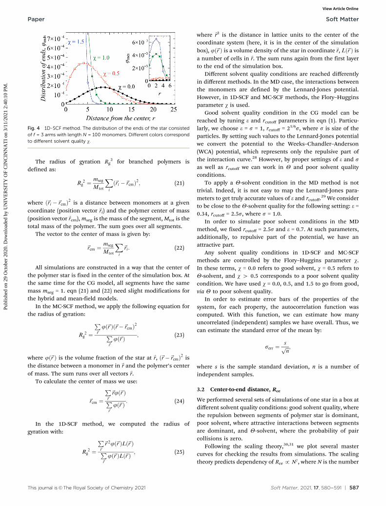
where f is the number of arms, rcenter-to-end,i is the distance fromthe center of the star to the end of the arm number i. eqn (19)can be applied to both CG and hybrid models because in CGthe positions of all segments at any time are available and inthe hybrid method the ends are also available. In the 1D-SCFmethod, instead of all positions of all segments, we have adistribution of the ends of the star. That is why eqn (19) is notused. A typical end-point distribution is presented in Fig. 4.Using this distribution we calculate the average distance of theends from the center with eqn (20):

Rce ¼X~r

rjendsð~r ÞLð~r Þjendsð~r ÞLð~r Þ

; (20)

where r is a distance from the center to a layer in sphericalgeometry, jendsð~r Þ is the volume density of the ends of the starin -

r, L(-r) is the number of cells in -r, sum goes from the first layer

to the end of the simulation box.

Soft Matter Paper

Publ

ishe

d on

29

Oct

ober

202

0. D

ownl

oade

d by

UN

IVE

RSI

TY

OF

CIN

CIN

NA

TI

on 3

/11/

2021

2:4

0:10

PM

. View Article Online

This journal is©The Royal Society of Chemistry 2021 Soft Matter, 2021, 17, 580--591 | 587

The radius of gyration Rg2 for branched polymers is

defined as:

Rg2 ¼ mseg

Mtot

Xi

~ri �~rcmð Þ2; (21)

where ~ri �~rcmð Þ2 is a distance between monomers at a givencoordinate (position vector -

ri) and the polymer center of mass(position vector -

rcm), mseg is the mass of the segment, Mtot is thetotal mass of the polymer. The sum goes over all segments.

The vector to the center of mass is given by:

~rcm ¼mseg

Mtot

Xi

~ri: (22)

All simulations are constructed in a way that the center ofthe polymer star is fixed in the center of the simulation box. Atthe same time for the CG model, all segments have the samemass mseg = 1. eqn (21) and (22) need slight modifications forthe hybrid and mean-field models.

In the MC-SCF method, we apply the following equation forthe radius of gyration:

Rg2 ¼

P~r

jð~r Þ ~r�~rcmð Þ2P~r

jð~r Þ ; (23)

where jð~r Þ is the volume fraction of the star at -r, ~r�~rcmð Þ2 is

the distance between a monomer in -r and the polymer’s center

of mass. The sum runs over all vectors -r.

To calculate the center of mass we use:

~rcm ¼

P~r

~rjð~r ÞP~r

jð~r Þ : (24)

In the 1D-SCF method, we computed the radius ofgyration with:

Rg2 ¼

P~r

~r 2jð~r ÞLð~r ÞP~r

jð~r ÞLð~r Þ ; (25)

where -r2 is the distance in lattice units to the center of the

coordinate system (here, it is in the center of the simulationbox), jð~r Þ is a volume density of the star in coordinate -

r, Lð~r Þ isa number of cells in -

r. The sum runs again from the first layerto the end of the simulation box.

Different solvent quality conditions are reached differentlyin different methods. In the MD case, the interactions betweenthe monomers are defined by the Lennard-Jones potential.However, in 1D-SCF and MC-SCF methods, the Flory–Hugginsparameter w is used.

Good solvent quality condition in the CG model can bereached by tuning e and rcutoff parameters in eqn (1). Particu-larly, we choose e = s = 1, rcutoff = 21/6s, where s is size of theparticles. By setting such values to the Lennard-Jones potentialwe convert the potential to the Weeks–Chandler–Anderson(WCA) potential, which represents only the repulsive part ofthe interaction curve.28 However, by proper settings of e and sas well as rcutoff we can work in Y and poor solvent qualityconditions.

To apply a Y-solvent condition in the MD method is nottrivial. Indeed, it is not easy to map the Lennard-Jones para-meters to get truly accurate values of e and rcutoff.29 We considerto be close to the Y-solvent quality for the following setting: e =0.34, rcutoff = 2.5s, where s = 1.0.

In order to simulate poor solvent conditions in the MDmethod, we fixed rcutoff = 2.5s and e = 0.7. At such parameters,additionally, to repulsive part of the potential, we have anattractive part.

Any solvent quality conditions in 1D-SCF and MC-SCFmethods are controlled by the Flory–Huggins parameter w.In these terms, w = 0.0 refers to good solvent, w = 0.5 refers toY-solvent, and w 4 0.5 corresponds to a poor solvent qualitycondition. We have used w = 0.0, 0.5, and 1.5 to go from good,via Y to poor solvent quality.

In order to estimate error bars of the properties of thesystem, for each property, the autocorrelation function wascomputed. With this function, we can estimate how manyuncorrelated (independent) samples we have overall. Thus, wecan estimate the standard error of the mean by:

serr ¼sffiffiffinp ;

where s is the sample standard deviation, n is a number ofindependent samples.

3.2 Center-to-end distance, Rce

We performed several sets of simulations of one star in a box atdifferent solvent quality conditions: good solvent quality, wherethe repulsion between segments of polymer star is dominant,poor solvent, where attractive interactions between segmentsare dominant, and Y-solvent, where the probability of paircollisions is zero.

Following the scaling theory,30,31 we plot several mastercurves for checking the results from simulations. The scalingtheory predicts dependency of Rce p Ng, where N is the number

Fig. 4 1D-SCF method. The distribution of the ends of the star consistedof f = 3 arms with length N = 100 monomers. Different colors correspondto different solvent quality w.

Paper Soft Matter

Publ

ishe

d on

29

Oct

ober

202

0. D

ownl

oade

d by

UN

IVE

RSI

TY

OF

CIN

CIN

NA

TI

on 3

/11/

2021

2:4

0:10

PM

. View Article Online

588 | Soft Matter, 2021, 17, 580--591 This journal is©The Royal Society of Chemistry 2021

of segments in an arm, g is a power which goes from g = 0.33 forpoor solvent to g = 0.588 for good solvent.

In Fig. 5 dependencies of center-to-end distance Rce areshown as a function of the number of segments N in the armof the star in different solvent quality conditions.

In Fig. 5a the dependency Rce is shown at good solventquality conditions. In agreement with scaling predictions,

all curves obey the scaling law for good solvent conditiong E 0.588. The 1D-SCF is the fastest method and gives thesmallest values for Rce for all lengths of star arms. Indeed,as it could be expected the MC-SCF method numericallyis in between 1D-SCF and MD methods. By reducing thenumber of explicit segments (pink curve), the results for Rce

become closer to the 1D-SCF method and deviate more fromMD. This shows indeed the MC-SCF bridges between mean-field 1D-SCF and exact’ MD results. It is interesting to see thatrelatively few explicit segments are needed to come close tothe MD results.

In Fig. 5b the dependency Rce is shown for the star atY-solvent conditions. Under theta conditions it is expectedthat the excluded volume effects are minor. Hence it is antici-pated that the values of Rce are relatively close to each other.In line with this we see a rather good agreement with thescaling prediction, g = 0.5 for all methods, and there are smallnumerical differences between MC-SCF and MD results. Againthe 1D-SCF underpredicts the value of Rce a bit more.

In Fig. 5c the dependency Rce is shown for the star at poorsolvent conditions. It can be observed, apart from 1D-SCFmethod, all methods predict the same result, which is consis-tent with scaling exponent g = 0.33.

In summary, the hybrid approach at good and theta solventquality conditions gives results that are intermediate betweenthose of the CG and the mean-field models. The differences inthe numerical coefficients are not very large and accountingfor the error bars all models show a satisfactory agreementone to another and importantly with the scaling predictions.In other words, by increasing the number of explicit segmentsin the MC-SCF hybrid (for sufficiently long arms) we can comecloser to the exact result, but this goes at the expense ofcomputational efficiency. When computational resources arelimited we may decide to reduce the number of explicitsegments and sacrifice some accuracy or vice versa.

3.3 Radius of gyration, Rg2

In Fig. 6a dependencies of the radius of gyration are shownas a function of the number of monomers per arm N for theMD, the MC-SCF, and the 1D-SCF methods at the good solventconditions. We see that all curves obey the scaling prediction ofg E 0.588 as well as Rg

2 E N1.18f 0.41 (our case f = 3 all times)fitted experimental data.2 Simultaneously, we compared ourresults with independent DPD simulations32 (not shown). Theslope of curves is consistent. The estimated error bars forMC-SCF and MD methods are mostly comparable, only forthe star with N = 200 segments per arm, the MD data looksundersampled, whereas the MC-SCF does not change thestraight line trend. Mean values of the radius of gyration Rg

2

in the MC-SCF and the 1D-SCF methods remain close to eachother for all set of arm lengths. The MD results stay slightlyhigher with respect to other methods.

In Fig. 6b the radius of gyration dependencies are shown forY-solvent conditions. The data from the MD and the MC-SCFmethods overlap. However, the 1D-SCF method gives slightlylower results. Moreover, the MC-SCF method with small number

Fig. 5ffiffiffiffiffiffiffiffiffiffiffiffiffiffiffiffiffiffiffiffiffiffiffiRce

2h i= b2h ip

of the star for MD, MC-SCF and 1D-SCF methods,where bhb2i is averaged bond length in MD and hb2i = 1 for MC-SCF and1D-SCF. Figure (a) represents data from simulations in a good solvent: MDparameters e = 1.0, rcutoff = 21/6, MC-SCF and 1D-SCF parameter w = 0.0.Figure (b) corresponds to Y-solvent: MD parameters e = 0.34, rcutoff = 2.5,MC-SCF and 1D-SCF parameter w = 0.5. Figure (c) Poor solvent qualityconditions: MD parameters e = 0.7, rcutoff = 2.5, MC-SCF and 1D-SCFparameter w = 1.5. The number of explicit segments in the MC-SCFmethod (green curve) could be calculated by (fN/n) + 1, where f = 3,n = 20. In MC-SCF with a small number of explicit segments (pink curve),the number of explicit segments equals 4 in the region N r 80, elsewhere 7.The shaded area represents the estimated error for the value.

Soft Matter Paper

Publ

ishe

d on

29

Oct

ober

202

0. D

ownl

oade

d by

UN

IVE

RSI

TY

OF

CIN

CIN

NA

TI

on 3

/11/

2021

2:4

0:10

PM

. View Article Online

This journal is©The Royal Society of Chemistry 2021 Soft Matter, 2021, 17, 580--591 | 589

of explicit segments gives results which represent the 1D-SCFresults, as one would expect. Taking the error bars into account,all models are in good agreement with each other.

Let us now consider the dependencies Rg2 at poor solvent

condition, given in Fig. 6c. For all arm lengths we see that theresults for the MD and the MC-SCF (both) methods are in goodcorrespondence and have slightly lower scaling exponent(about g = 0.3). The minor numerical differences betweenthe models are similar to the ones found for theta solvent.

The 1D-SCF method shows an exponent g = 0.33 which is thevalue expected from scaling theory.

3.3.1 Polymer density profile. In Fig. 7 we present thepolymer density profile, that is the volume fraction j as afunction of distance from the center of the polymer star forN = 160 segments per arm.

The polymer density profile at good solvent is shown on theleft hand side of the Fig. 7. The MD and the MC-SCF resultsobey the scaling prediction33,34 r�4/3 better than results fromthe 1D-SCF method. The 1D-SCF result has the strongestdeviation from the scaling prediction. Simultaneously, wecompared our results with independent simulations (notshown).2,35 The slope and values were in good agreement.

The polymer density profile at Y-solvent is depicted in thecenter of Fig. 7. Apart from the small distances, all methods arein good agreement one to another. The density profiles obey thescaling prediction j(r) p r�1 only for small distances from thecenter of the polymer star.33,34

On the right hand side of Fig. 7 the polymer density profilesare presented at poor solvent conditions. The MC-SCF (both)and the MD methods are in good mutual agreement all valuesof r. However, the 1D-SCF does not follow the same trend.The 1D-SCF method predicts that the star at poor solvent iscollapsed to a higher density and extends less far in thesolution. Clearly, the 1D-SCF underpredicts the fluctuations(in the interfacial region between the globule and the solvent)in this case.

3.3.2 Efficiency. In order to give quantitative estimation ofefficiency of the MD and the MC-SCF methods, we provideestimation of integrated autocorrelation time for Rce values.In Fig. 8 we present estimation of the lag t as a functionof length of the star arm N, calculated accordingly themanuscript.36 We provide estimations for different solvent

Fig. 6ffiffiffiffiffiffiffiffiffiffiffiffiffiffiffiffiffiffiffiffiffiffiffiRg

2� ��

b2h iq

of the star for MD, MC-SCF and SCF methods, wherehb2i is averaged bond length in MD and hb2i = 1 for MC-SCF and 1D-SCF.Figure (a) Good solvent quality condition: MD parameters e = 1.0, rcutoff =21/6, MC-SCF and 1D-SCF parameter w = 0.0. Figure (b) Y-solvent qualitycondition: MD parameters e = 0.34, rcutoff = 2.5, MC-SCF and 1D-SCFparameter w = 0.5. Figure (c) Poor solvent quality conditions: MD para-meters e = 0.7, rcutoff = 2.5, MC-SCF and 1D-SCF parameter w = 1.5. Thenumber of explicit segments in the MC-SCF method could be calculatedby (fN/n) + 1, where f = 3, n = 20. The shaded area represents theestimated error for the value.

Fig. 7 The polymer density profile j(r) for polymer stars with N = 160 andf = 3 found by the MC-SCF (green n = 20, pink n = 80), the MD (black) andthe 1D-SCF methods (red). (Left) Good solvent condition: MD parameterse = 1.0, rcutoff = 21/6, MC-SCF and 1D-SCF parameter w = 0.0. (Center)Y-solvent condition: MD parameters e = 0.34, rcutoff = 2.5, MC-SCF and1D-SCF parameter w = 0.5. (Right) Poor solvent condition: MD parameterse = 0.7, rcutoff = 2.5, MC-SCF and 1D-SCF parameter w = 1.5. The number ofexplicit segments in the MC-SCF (green curve) method is 25, for theMC-SCF method with a small number of explicit segments (pink curve) is 7.The shaded area represents the estimated error for the value.

Paper Soft Matter

Publ

ishe

d on

29

Oct

ober

202

0. D

ownl

oade

d by

UN

IVE

RSI

TY

OF

CIN

CIN

NA

TI

on 3

/11/

2021

2:4

0:10

PM

. View Article Online

590 | Soft Matter, 2021, 17, 580--591 This journal is©The Royal Society of Chemistry 2021

qualities. We can see that the MD method works more efficientfor poor solvent than for other solvent conditions, whereas, theMC-SCF method gives even smaller lag for all solvent qualityconditions (less than 100 MC-SCF steps).

At good and Y solvent conditions, we can observe that withincreasing segments per arm N the MD method degradates.Namely, the MD method becomes less efficient with specificMD step (our case was 150), whereas the MC-SCF slightlyfluctuates around zero slope. However, we need to distinguishthe MC-SCF step and the MD step. The important idea here isthe time restriction for the system (24 h), which leads to thesuperiority of one method over another assuming machineryconstrain (the same computational power).

At poor solvent condition, the MC-SCF slightly degradates atbig lengths of star arms. However, the MC-SCF method still hasbig gap to the MD best lag.

4 Conclusions

We compared the MC-SCF method based on a combination ofMonte Carlo and the SF-SCF technique with methods based onpurely coarse-grained (MD) and purely mean-field models(1-gradient SF-SCF). We employed these methods on the polymerstar and we focused on the size characteristics as well as thepolymer density profile of a polymer star. We compared thepredictive abilities of these models at different solvent qualityconditions: good solvent, Y-solvent, and poor solvent.

All models showed consistent results. The MD method(purely coarse-grained model) is the most ‘exact’ method thatgives reliable results, however it quickly becomes computation-ally expensive to produce simulation results of proper statisticalquality. The 1D-SCF method (purely mean-field model) iscomputationally less expensive in the whole range of solventqualities. In all cases, 1-gradient SF-SCF method produced anunderestimation of the properties of the system. The MC-SCFmethod, on the one hand, suppresses the effect of the mean-fieldapproximation by introducing a small number of explicit (CG)

segments and, on the another hand, not as much expensive as theMD method (within the time and machinery constraints).

We focused on quantities such as the center-to-end distanceRce, the radius of gyration Rg

2, and the polymer densityprofile j(r). These quantities were compared to scalingpredictions2,33,34 and typically they were in line with these.Within the statistical errors, the various methods were alsoconsistent with each other. Only minor deviations occurred forshort arm lengths.

We estimated the efficiencies of the methods by estimatingthe integrated autocorrelation time t for Rce values. We showedthat the MD method degrades much faster than the MC-SCFwith increasing number of segments per arm N. This provedthat the MC-SCF method is computationally more efficient.

We found that the MC-SCF method with pivot, one-bondand one-node movements can successfully sample all solventconditions. The relatively low number of explicitly simulateddegrees of freedom in the hybrid model makes it more efficientas compared to the purely CG model (MD). Moreover, byvarying the number of explicitly represented segments in thehybrid model, the MC-SCF method can be tuned to a suitablecompromise between the detail of the resolution andcomputational cost.

Hence, our results demonstrated that the MC-SCF method isa good trade-off between the efficient 1D-SCF method and theexplicit-particle representation of the MD method. In Y-solventcondition, results of all methods are in close correspondence.In good solvent conditions, the MC-SCF method was shown tobe superior to the pure 1D-SCF method. The MC-SCF methodwith a necessary and sufficient amount of explicit segments is

numerically closer to ‘exact’ MDffiffiffiffiffiffiffiffiffiffiffiffiffiRce

2h ip

;ffiffiffiffiffiffiffiffiffiffiffiffiRg

2� �q� �

, and j(r).

At poor solvent, the MC-SCF method was superior additionally tothe MD method too, in terms of generating the (uncorrelated)samples.

This overall behavior and its tunable inheritance make theMC-SCF method an interesting option for molecular modelingof macromolecular systems. The method can easily be extendedto a collection of stars in a solvent, or to end-grafted chains on asurface (brush).

Conflicts of interest

There are no conflicts to declare.

Acknowledgements

AK would like to thank his friend Aleksandr Chudov forproductive discussions at very early stage. AK thanks the secondanonymous reviewer for helpful comments on steady stages ofthe manuscript. This work was supported by the GrantAgency of Charles University (project 318120). This work wassupported by the Czech Science Foundation, grant 17-02411Y.The access to computing facilities of National Grid Infrastruc-ture MetaCentrum (LM2015042) and CERIT Scientific Cloud(LM2015085) is appreciated.

Fig. 8 The estimated integrated autocorrelation time t as a function ofnumber of segments per arm N. Good solvent condition: MD parameterse = 1.0, rcutoff = 21/6, MC-SCF parameter w = 0.0. Y-Solvent condition: MDparameters e = 0.34, rcutoff = 2.5, MC-SCF parameter w = 0.5. Poor solventcondition: MD parameters e = 0.7, rcutoff = 2.5, MC-SCF parameter w = 1.5.

Soft Matter Paper

Publ

ishe

d on

29

Oct

ober

202

0. D

ownl

oade

d by

UN

IVE

RSI

TY

OF

CIN

CIN

NA

TI

on 3

/11/

2021

2:4

0:10

PM

. View Article Online

This journal is©The Royal Society of Chemistry 2021 Soft Matter, 2021, 17, 580--591 | 591

References

1 G. W. Slater, C. Holm, M. V. Chubynsky, H. W. de Haan,A. Dube, K. Grass, O. A. Hickey, C. Kingsburry, D. Sean,T. N. Shendruk and L. Zhan, Electrophoresis, 2009, 30,792–818.

2 G. S. Grest, L. J. Fetters, J. S. Huang and D. Richter, Advances inChemical Physics: Polymeric Systems, 2007, vol. 94, pp. 67–163.

3 C. N. Likos, Phys. Rep., 2001, 348, 267–439.4 Y. Zhao, S. M. Ma, B. Li, A. De Nicola, N. S. Yu and B. Dong,

Polymers, 2019, 11, 1–16.5 A. De Nicola, T. Kawakatsu and G. Milano, Macromol. Chem.

Phys., 2013, 214, 1940–1950.6 J. Bergsma, J. van der Gucht and F. A. Leermakers, Macromol.

Theory Simul., 2019, 28, 1–14.7 E. Sarukhanyan, A. De Nicola, D. Roccatano, T. Kawakatsu

and G. Milano, Chem. Phys. Lett., 2014, 595–596, 156–166.8 G. J. Sevink, F. Schmid, T. Kawakatsu and G. Milano, Soft

Matter, 2017, 13, 1594–1623.9 Y. L. Zhu, Z. Y. Lu, G. Milano, A. C. Shi and Z. Y. Sun, Phys.

Chem. Chem. Phys., 2016, 18, 9799–9808.10 J. Bergsma, F. A. Leermakers and J. Van Der Gucht, Phys.

Chem. Chem. Phys., 2015, 17, 9001–9014.11 B. J. Reynwar, G. Illya, V. A. Harmandaris, M. M. Muller,

K. Kremer and M. Deserno, Nature, 2007, 447, 461–464.12 P. Kosovan, J. Kuldova, Z. Limpouchova, K. Prochazka,

E. B. Zhulina and O. V. Borisov, Soft Matter, 2010, 6,1872–1874.

13 F. Weik, R. Weeber, K. Szuttor, K. Breitsprecher, J. de Graaf,M. Kuron, J. Landsgesell, H. Menke, D. Sean and C. Holm,Eur. Phys. J.-Spec. Top., 2019, 227, 1789–1816.

14 J. E. Jones, Proc. R. Soc. A, 1924, 106, 463–477.15 H. R. Warner, Ind. Eng. Chem. Fundam., 1972, 11, 379–387.16 G. J. Fleer, M. A. C. Stuart, J. M. H. M. Scheutjens,

T. Cosgrove and B. Vincent, Polymers at Interfaces, Springer,1993.

17 O. V. Borisov, E. B. Zhulina, F. A. Leermakers, M. Ballauffand A. H. Muller, Advances in Polymer Science, SpringerBerlin, Heidelberg, 2011, vol. 241, pp. 1–55.

18 O. Rud, T. Richter, O. Borisov, C. Holm and P. Kosovan,Soft Matter, 2017, 13, 3264–3274.

19 J. M. Scheutjens and G. J. Fleer, J. Phys. Chem., 1979, 83,1619–1635.

20 M. Mocan, M. Kamperman and F. A. Leermakers, Polymers,2018, 10, 78.

21 F. A. M. Leermakers, J. Scheutjens and J. Lyklema, Biophys.Chem., 1983, 18, 353–360.

22 J. Bergsma, F. A. M. Leermakers, J. M. Kleijn and J. van derGucht, J. Chem. Theory Comput., 2018, 14, 6532–6543.

23 M. Charlaganov, P. Kosovan and F. A. Leermakers, Soft Matter,2009, 5, 1448–1459.

24 Z. Preisler, P. Kosovan, J. Kuldova, F. Uhlık, Z. Limpouchova,K. Prochazka and F. A. Leermakers, Soft Matter, 2011, 7,10258–10265.

25 O. A. Evers, J. M. H. M. Scheutjens and G. J. Fleer, Macro-molecules, 1991, 24, 5558–5566.

26 L. D. Gelb, J. Chem. Phys., 2003, 118, 7747–7750.27 N. Metropolis, A. W. Rosenbluth, M. N. Rosenbluth, A. H.

Teller and E. Teller, J. Chem. Phys., 1953, 21, 1087–1092.28 J. D. Weeks, D. Chandler and H. C. Andersen, J. Chem. Phys.,

1971, 54, 5237–5247.29 U. Micka, C. Holm and K. Kremer, Langmuir, 1999, 15,

4033–4044.30 R. Guida and J. Zinn-Justin, J. Phys. A: Math. Gen., 1998, 31,

8103–8121.31 N. Clisby, Phys. Rev. Lett., 2010, 104, 1–4.32 M. M. Nardai and G. Zifferer, J. Chem. Phys., 2009, 131, 124903.33 M. Daoud and J. P. Cotton, J. Phys., 1982, 43, 531–538.34 E. B. Zhulina, T. M. Birshtein and O. V. Borisov, Eur. Phys.

J. E: Soft Matter Biol. Phys., 2006, 20, 243–256.35 A. D. Cecca and J. J. Freire, Macromolecules, 2002, 35, 2851–2858.36 U. Wolff, Comput. Phys. Commun., 2004, 156, 143–153.

Paper Soft Matter

Publ

ishe

d on

29

Oct

ober

202

0. D

ownl

oade

d by

UN

IVE

RSI

TY

OF

CIN

CIN

NA

TI

on 3

/11/

2021

2:4

0:10

PM

. View Article Online