Computer Graphics - Week 12 - Department of …feiner/courses/csw4160/slides/S99-12.pdfComputer...

Computer Graphics - Week 12Computer Graphics - Week 12

Bengt-Olaf SchneiderBengt-Olaf SchneiderIBM T.J. Watson Research CenterIBM T.J. Watson Research Center

© Bengt-Olaf Schneider, 1999Computer Graphics – Week 12

Questions about Last Week ?Questions about Last Week ?


Overview of Week 12Overview of Week 12

Graphics HardwareOutput devices (CRT and LCD)Graphics architecturesPerformance modeling

ColorColor theoryColor gamutsGamut matchingColor spaces (next week)


Graphics Hardware: OverviewGraphics Hardware: Overview

Display technologies

Graphics architecture fundamentals

Many of the general techniques discussed earlier in the semester were developed with hardware in mind

Close similarity between software and hardware architectures


Display TechnologiesDisplay Technologies

CRT (Cathode Ray Tube)

LCD (Liquid Crystal Display)


CRT: Basic Structure (1)CRT: Basic Structure (1)

Electron Beam

Cathode

Control Grid

Electron Lens

VerticalDeflectionSystem

HorizontalDeflectionSystem

CollectorElectrode

Phosphor

Top View


CRT: Basic Structure (2)CRT: Basic Structure (2)

Electron Beam

Cathode

Control Grid

Electron Lens

VerticalDeflectionSystem

HorizontalDeflectionSystem

CollectorElectrode

Phosphor

Deflection SystemTypically magnetic and not electrostaticReduces the length of the tube and allows wider deflection angles

PhosporFluorescence: Light emitted after impact of electronsPersistence: Duration of emission after beam is turned off. Determines flicker properties of the CRT.


CRT: Scan PatternCRT: Scan Pattern

1 1

2 8

3 2

4 9

5 3

6 107 4

8 119 5

10 1211 6

12 13

13 7

14 14

(a) (b)

Non-interlacedA.k.a. progressiveUsed in computer displays

InterlacedUsed in standard TVsWorks because of irregular nature of TV imagesHorizontal patterns flicker


CRT: Shadow MaskCRT: Shadow Mask

Shadow mask

Screen

Electron guns

For color CTRs, beam must focus exactly on the phosphor to avoid cross-talk between pixels

Shadow mask blocks off parts of the beam outside the pixelCreates sharper imageAllows for wider deflection angles (and shorter tubes).Requires careful registration of mask with phosphor


CRT: Phosphor ArrangmentsCRT: Phosphor Arrangments

R

G B

R

G B

R

G B

R

G BR

G B

R

G B

R

G B

R

G BR RG GB B

(a) (b)

Pi PiPd

Delta arrangementHigh-quality monitorsPd approx. 0.2 mm

Inline arrangementTV monitorsPi approx. 0.6 mm


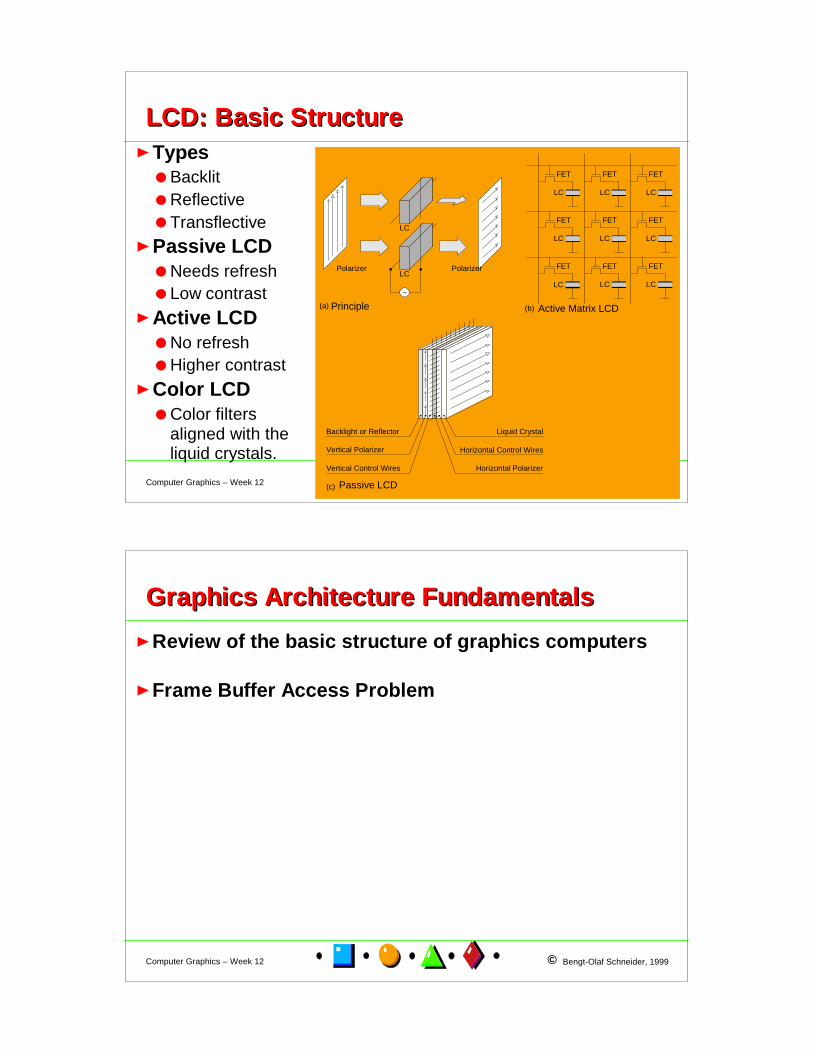
TypesBacklitReflectiveTransflective

Passive LCDNeeds refreshLow contrast

Active LCDNo refreshHigher contrast

Color LCDColor filters aligned with the liquid crystals.

LCD: Basic StructureLCD: Basic Structure

~

(a)

Polarizer PolarizerLC

LC

Backlight or Reflector

Vertical Polarizer

Vertical Control Wires

Liquid Crystal

Horizontal Control Wires

Horizontal Polarizer

(c)

LC

LC

LC

LC

LC

LC

LC

LC

LC

FET

FET

FET

FET

FET

FET

FET

FET

FET

(b)Principle Active Matrix LCD

Passive LCD


Graphics Architecture FundamentalsGraphics Architecture Fundamentals

Review of the basic structure of graphics computers

Frame Buffer Access Problem


Graphics ComputersGraphics Computers

Host CPU GraphicsSubsystem

InputDevices

OutputDevice

HostOperating systemApplication softwareInput device polling/interruptsGeneration of graphics data

Graphics SubsystemReceive graphics data and commands from hostGenerate and refresh image on the output device


Graphics SubsystemGraphics Subsystem

Geometric OperationsOperates on graphics primitives, e.g. trianglesTypically in floating pointBasic steps:

Modeling + viewing transformationsModeling + viewing transformationsLightingLightingClippingClippingPerspective transformationsPerspective transformationsViewport mappingViewport mapping

Image GenerationDifferent for raster and vectorTypically in fixed pointConversion of screen-space primitives into pixels / strokes

Screen refreshFor volatile displays (CRT)Illusion of standing image

GeometricOperations

ImageGeneration

ScreenRefresh

Bandwidth


Raster Graphics SystemsRaster Graphics SystemsRaster graphics systems have replaced vector graphics system everywhere but in niche applications, e.g. radarPrincipal advantages over vector displays are

ability to display images of arbitrary complexity without flickerdisplay of shaded images instead of wireframes

Frame Buffer is the key architectural component of every raster system.

Provides storage for every pixel valueUpdated by rasterizer or CPURead by video controller for screen refresh

Frame buffer access problem as a result of contention between rasterizer and refresh.


Raster Graphics Subsystem: ReviewRaster Graphics Subsystem: Review

ClippingLightingCalculations

ModelingTransforms

ViewingTransforms

Geometric Operations

Image Generation

SetupCalculations

ScreenRefresh

FrameBufferRasterization Pixel

Processing

Perspective+ Viewport

SetupPer-primitive calculations to initialize the rasterizationE.g. slopes of edges

RasterizationBreak object into pixelsAssign pixel values

Pixel-processingModifies generated pixel values with already stored pixel values, e.g. texture mapping or blendingStoring of pixel value into the frame buffer


Screen RefreshScreen Refresh

Required for non-persistent display devicesCreates illusion of standing imageRefresh rate

Minimum approx 30 HzErgonomic standards require 80+ Hz

Refresh logic Continuously reads the frame buffer in scanline orderConverts the pixel values into analog signals for monitor


Video Controller: True ColorVideo Controller: True Color

x

y

R G B12864 23

DA

DA

DA

Frame Buffer

Pixel Contents

Screen

Digital-AnalogConverters


Video Controller: Color MapVideo Controller: Color Map

x

y

DA

DA

DA

Frame BufferScreen

Digital-AnalogConverters

64 128 23i

Look-up Table


Screen Refresh: Pixel TimingScreen Refresh: Pixel Timing

Pixel time:

H

tVtf

thv

rpixel

−

−

=

1

pixelr t

B bpp=

Bandwidth:

H x V x bpp fr [Hz] th [usec] tv [usec] tpixel [nsec] Br [MB/sec]

512 x 512 x 1 60 6.62 1250 45.88 21.8

1024 x 768 x 2 60 4.0 593 16.53 121.0

1280 x 1024 x 3 60 4.0 596 9.14 328.2

th

tv

Active Time (H x V)

Vertical Retrace

Hor

izon

tal R

etra

ce 1/fr


Frame Buffer Access ProblemFrame Buffer Access ProblemPixel access time during refresh(10-50 nsec) is much shorter than typical DRAM cycle times (100-200 nsec).Rasterizer and screen refresh compete for access to the frame buffer ... and the rasterizer always loses.

Therefore:The frame-buffer memory bandwidth must be increasedRasterizer accesses and screen refresh must be decoupled

Solutions:Seminconductor technology

Access modes and different memory types, e.g. VRAM, FBRAM, TEXRAMAccess modes and different memory types, e.g. VRAM, FBRAM, TEXRAM

Frame-buffer architectureMulti-bank memory, Double-buffering Multi-bank memory, Double-buffering


Frame Buffer: Bandwidth BudgetFrame Buffer: Bandwidth Budget

Example:64-bit memory interface50 nsec/Byte access time (20 MHz)Bandwidth = 160 MBytes/sec

Screen: 1280 x 1024 x 8bppRefresh rate: 60 HzRefresh bandwidth = 110 MBytes/sec

Bandwidth budget:31.25% rasterizer68.75% screen refresh

Refresh Rasterizer


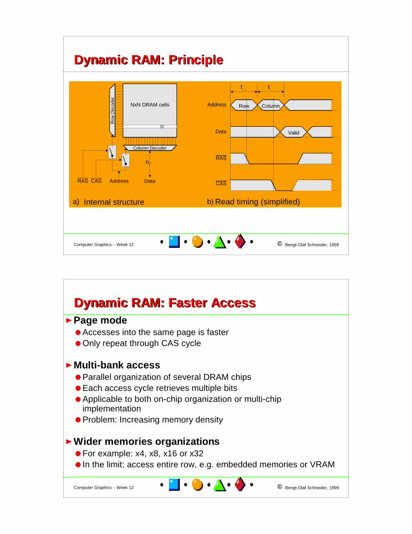
Dynamic RAM: PrincipleDynamic RAM: Principle

Address Data

Column Decoder

Row

Dec

oder

NxN DRAM cells

RAS CAS

Address

Data

RAS

CAS

Row Column

Valid

tr o w

tc o l

n

a) b)Internal structure Read timing (simplified)


Dynamic RAM: Faster AccessDynamic RAM: Faster AccessPage mode

Accesses into the same page is fasterOnly repeat through CAS cycle

Multi-bank accessParallel organization of several DRAM chipsEach access cycle retrieves multiple bitsApplicable to both on-chip organization or multi-chip implementationProblem: Increasing memory density

Wider memories organizationsFor example: x4, x8, x16 or x32In the limit: access entire row, e.g. embedded memories or VRAM


Video RAMVideo RAM

Dual-ported memory

Load entire row in one cycle into the shift register

Shift register I/O is independent from main port I/O

Bandwidth budget:

Refresh Rasterizer

Row

Dec

ode

Col. Decode

Shift Register

Row Addr

Column Addr

Serial I/O8

9

9

512

512

512

Data I/O8

1024 x 1024DRAM Array


Double BufferingDouble Buffering

Frame buffer bandwidthScreen refreshImage generation

Double-buffering decouples image generation from screen refresh

Front buffer always contains a complete image while back buffer is rebuilt

Buffer A

Buffer BSw1 Sw2


Summary of Key ConceptsSummary of Key Concepts

Classification criteria for displays

Principles of operation for CRTs and LCDs

Basic structure of graphics systems, both vector and raster displays

Data flow through and function of each block in raster displays

Host CPU - Rasterizer - Frame buffer - Screen refresh

Frame-buffer design objectives and solutions


Computational and Bandwidth DemandsComputational and Bandwidth Demands

Computational ComplexityFloating-point vs. Fixed-point (integer) operationsTypes of operation (add/subtract, multiply, divide)Memory accesses (read / write)

Bandwidth = Data / Time [MB/sec, Mb/sec]Applies to speed with which datapath components can process, transmit or access dataMemory bandwidth is often criticalOther datapath elements: processors, busses, D/A converters


Raster Graphics SubsystemRaster Graphics Subsystem

ClippingLightingCalculations

ModelingTransforms

ViewingTransforms

Geometric Operations

Image Generation

SetupCalculations

ScreenRefresh

FrameBufferRasterization Pixel

Processing

Perspective+ Viewport

SetupPer-primitive calculations to initialize the rasterizationE.g. slopes of edges

RasterizationBreak object into pixelsAssign pixel values

Pixel-processingModifies generated pixel values with already stored pixel values, e.g. texture mapping or blendingStoring of pixel value into the frame buffer


Per-triangle OperationsPer-triangle Operations

Step Addition Multiplication Division Conversion

Setup

Rasterization 9 3 3

Attributes 5 + 5a 2 + 3a 1 1

Total 14 + 5a 2 + 3a 4 4

23 + 10a instructions/pixel(a is the number of attributes to be interpolated across the triangle)


Per-vertex OperationsPer-vertex Operations

130 + 5a + 16L instructions/pixel

Step Addition Multiplication Division Exponentiation

Model transform 16 25

Phong lighting 6L 3 + 9L L

View transform 12 16

Clipping 21 + 3a 18 + 2a 12

Perspective xform 2 1

Viewport mapping 2 2

Total 51 + 3a + 6L 66 + 2a + 9L 13 L


Per-span OperationsPer-span Operations

Rasterization: 3+a Additions/span


Per-pixel OperationsPer-pixel Operations

Step Addition Multiplication Division Read Write

Rasterization 2+a

Z-test 1 1

Buffer Clear 2(HxV)

Texture Mapping 1 / 2 / 4 / 8

Persp. Division 2

LOD Calculation 7 10 1

Filtering 0 / 2 / 6 / 14 0 / 1 / 3 / 7

Update 2

Total 6.5 / 7.5 / 9.5 / 13.5 + a

5 / 5.5 / 6.5 / 8.5 1.5 1.5 / 2 / 3 / 5 1 + 2(HxV)

x0.513 / 14.5 / 17.5 / 23.5 + a instructions/pixel2.5 / 3 / 4 / 6 + 2(HxV) memory accesses per pixel


Summary: OperationsSummary: Operations

Per vertex: 130+5a+16L

Per triangle: 23 + 10a

Per span: 3 + a

Per pixel: 13 / 14 / 17.5 / 23.5 + a


Performance Model (1)Performance Model (1)

0TTnTnTnTnT ppssvvtt +⋅+⋅+⋅+⋅=T Total rendering time [sec]Tt Rendering time per triangle [sec/triangle]Tv Rendering time per vertex [sec/vertex]Ts Rendering time per span [sec/span]Tp Rendering time per pixel [sec/pixel]T0 Rendering time overhead [sec] nt Number of triangles

nvNumber of verticesnsNumber of spansnpNumber of pixels


Performance Model (2)Performance Model (2)

0TTnTnTnTnT ppssvvtt +⋅+⋅+⋅+⋅=

Linear approximation of the true performance characteristics

Ignores 2nd order effectsCache/page missesCache/page missesContention for shared resources like busses or memory Contention for shared resources like busses or memory

Linear model is useful in many practical applicationsPerformance characterization, e.g. benchmarkingPerformance characterization, e.g. benchmarkingPerformance prediction, e.g. adaptive systemsPerformance prediction, e.g. adaptive systems


Data RepresentationData RepresentationColors: Integer

24 bits (8-8-8)8 bits (color index mode)

Depth: Integer16, 24, 32 bits

Texture coordinates: Integer

16 bits

Texture values: Integer1, 4, 8 bits (color indices)16, 24 (5-6-5, 8-8-8)

Slopes: Fixed pointInteger: Maximum pixel addressFraction: Maximum pixel address


Bandwidth in the Raster PipelineBandwidth in the Raster Pipeline

As data travel through the raster pipeline, data are described at increasingly lower levels of abstraction

Application: High-level objects, procedural objectsGeometry pipeline: triangles, polygons, text, ...Setup stage: TrianglesRasterization: Simple triangles, edges, slopesPixel processing: Pixel fragmentsFrame buffer: Pixels

Therefore, the same information is described less concisely

The bandwidth in the raster pipeline must increase along the pipeline in order to avoid pipeline stalls


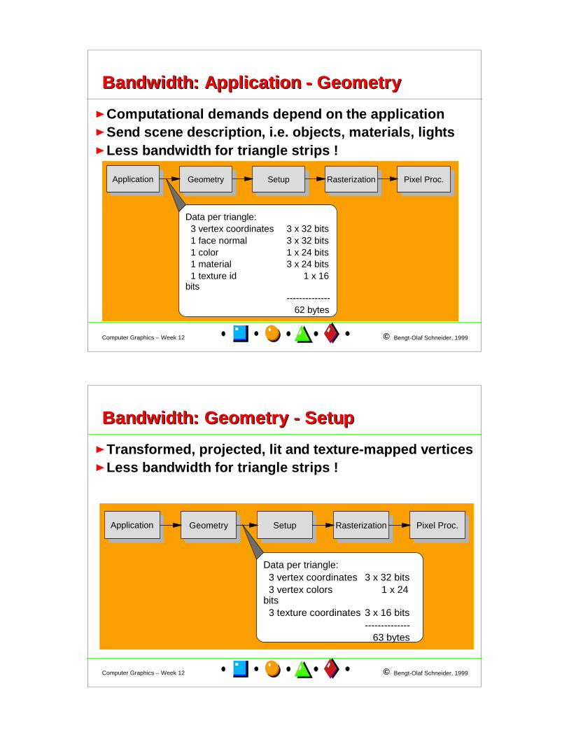
Bandwidth: Application - GeometryBandwidth: Application - Geometry

Computational demands depend on the applicationSend scene description, i.e. objects, materials, lightsLess bandwidth for triangle strips !

Application Pixel Proc.RasterizationSetupGeometry

Data per triangle: 3 vertex coordinates 3 x 32 bits 1 face normal 3 x 32 bits 1 color 1 x 24 bits 1 material 3 x 24 bits 1 texture id 1 x 16 bits --------------

62 bytes


Bandwidth: Geometry - SetupBandwidth: Geometry - Setup

Transformed, projected, lit and texture-mapped verticesLess bandwidth for triangle strips !


Data per triangle: 3 vertex coordinates 3 x 32 bits 3 vertex colors 1 x 24 bits 3 texture coordinates 3 x 16 bits --------------

63 bytes


Bandwidth: Setup - RasterizationBandwidth: Setup - Rasterization

Compute edge slopes and plane equations


Data per triangle: 3 vertex coordinates 3 x 16 bits 3 vertex colors 1 x 24 bits 3 texture coordinates 3 x 16 bits 3 edge slopes (dx/dy) 1 x 32 bits 1 depth par (dz/dx,y) 2 x 32 bits 3 color par's (drgb/dx,y)2 x 16 bits 3 texture par's (dto.) 2 x 32 bits --------------

101 bytes


Bandwidth: Rasterizer - Pixel Proc.Bandwidth: Rasterizer - Pixel Proc.

Generate pixels covered by triangle


Data per pixel: 1 pixel coordinate 2 x 16 bits 1 pixel depth 1 x 16 bits 1 pixel color 3 x 8 bits 1 texture coordinate 2 x 16 bits --------------

13 bytes


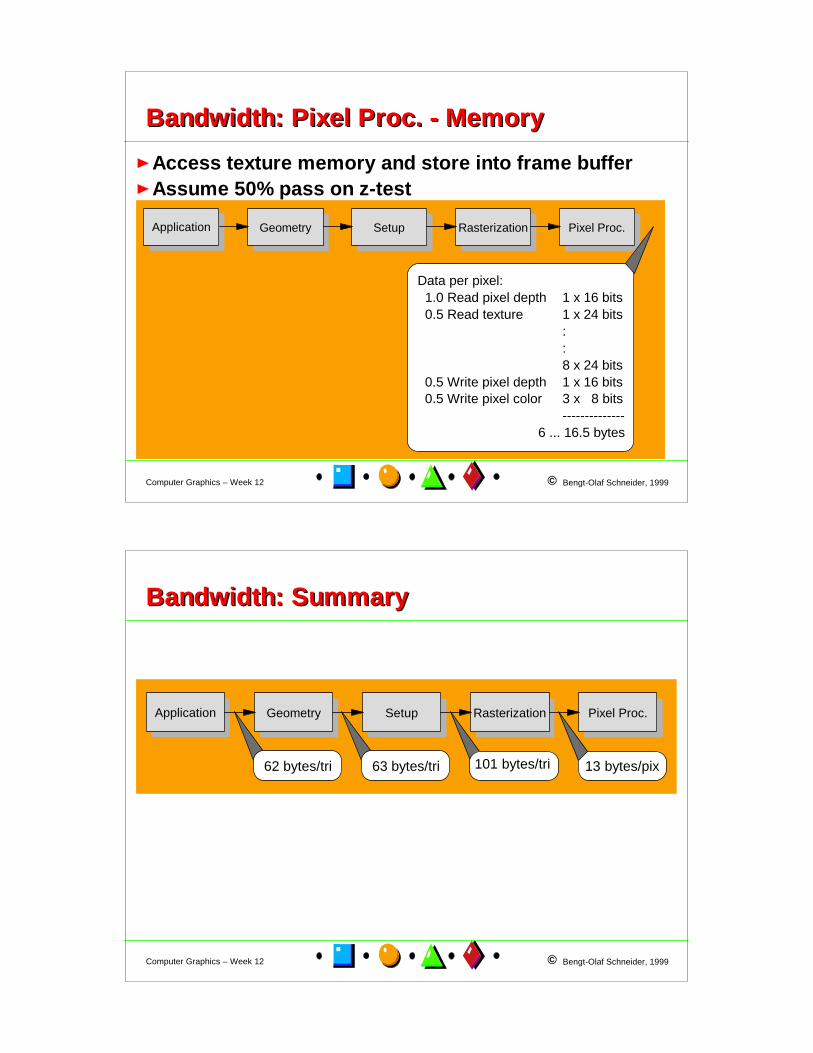
Bandwidth: Pixel Proc. - MemoryBandwidth: Pixel Proc. - Memory

Access texture memory and store into frame bufferAssume 50% pass on z-test


Data per pixel: 1.0 Read pixel depth 1 x 16 bits 0.5 Read texture 1 x 24 bits

: :

8 x 24 bits 0.5 Write pixel depth 1 x 16 bits 0.5 Write pixel color 3 x 8 bits --------------

6 ... 16.5 bytes


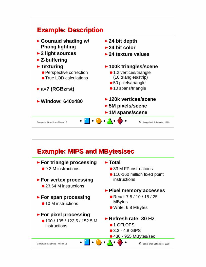
Bandwidth: SummaryBandwidth: Summary


62 bytes/tri 13 bytes/pix63 bytes/tri 101 bytes/tri


Example: DescriptionExample: Description

Gouraud shading w/ Phong lighting2 light sourcesZ-bufferingTexturing

Perspective correctionTrue LOD calculations

a=7 (RGBzrst)

Window: 640x480

24 bit depth24 bit color24 texture values

100k triangles/scene1.2 vertices/triangle (10 triangles/strip)50 pixels/triangle10 spans/triangle

120k vertices/scene5M pixels/scene1M spans/scene


Example: MIPS and MBytes/secExample: MIPS and MBytes/sec

For triangle processing9.3 M instructions

For vertex processing23.64 M instructions

For span processing10 M instructions

For pixel processing100 / 105 / 122.5 / 152.5 M instructions

Total33 M FP instructions110-160 million fixed point instructions

Pixel memory accessesRead: 7.5 / 10 / 15 / 25 MBytesWrite: 6.8 MBytes

Refresh rate: 30 Hz1 GFLOPS3.3 - 4.8 GIPS430 - 955 MBytes/sec


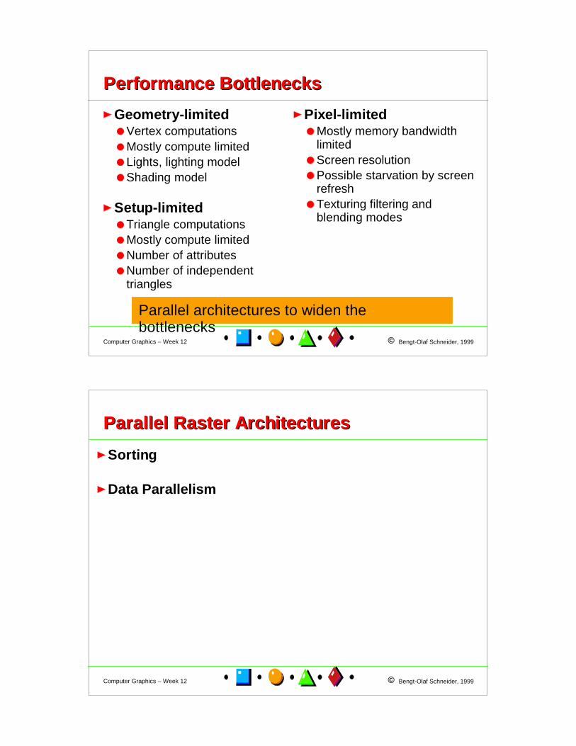
Parallel architectures to widen the bottlenecks

Performance BottlenecksPerformance Bottlenecks

Geometry-limitedVertex computationsMostly compute limitedLights, lighting modelShading model

Setup-limitedTriangle computationsMostly compute limitedNumber of attributesNumber of independent triangles

Pixel-limitedMostly memory bandwidth limitedScreen resolutionPossible starvation by screen refreshTexturing filtering and blending modes


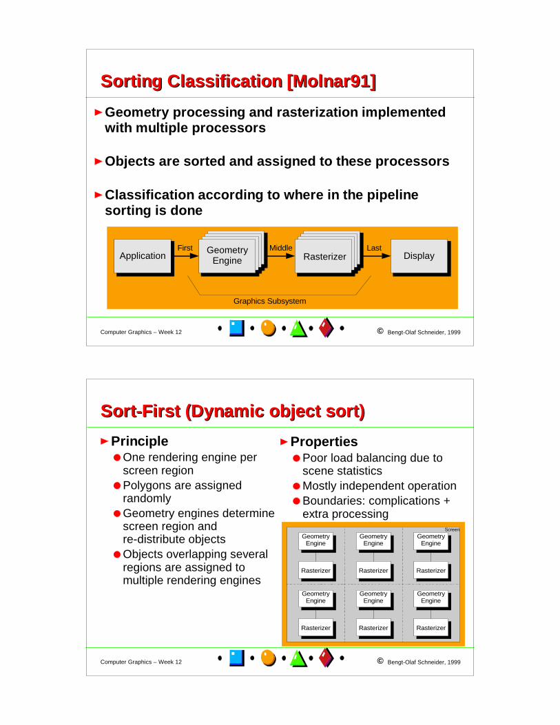
Parallel Raster ArchitecturesParallel Raster Architectures

Sorting

Data Parallelism


Sorting Classification [Molnar91]Sorting Classification [Molnar91]

Geometry processing and rasterization implemented with multiple processors

Objects are sorted and assigned to these processors

Classification according to where in the pipeline sorting is done

GeometryEngine RasterizerApplication Display

First Middle Last

Graphics Subsystem


Sort-First (Dynamic object sort)Sort-First (Dynamic object sort)

GeometryEngine

Rasterizer

GeometryEngine

Rasterizer

GeometryEngine

Rasterizer

GeometryEngine

Rasterizer

GeometryEngine

Rasterizer

GeometryEngine

Rasterizer

Screen

PrincipleOne rendering engine per screen regionPolygons are assigned randomlyGeometry engines determine screen region and re-distribute objectsObjects overlapping several regions are assigned to multiple rendering engines

PropertiesPoor load balancing due to scene statisticsMostly independent operationBoundaries: complications + extra processing


Sort-Middle (Screen subdivision)Sort-Middle (Screen subdivision)Geometry

EngineGeometry

EngineGeometry

EngineGeometry

Engine

Rasterizer

Rasterizer Rasterizer Rasterizer

Rasterizer Rasterizer

Screen

PrincipleRasterizers are statically assigned to screen regionsObjects are randomly assigned to geometry enginesGE transfer transformed objects to proper rasterizer

PropertiesDistributed databaseDoesn't maintain object orderingHigh latency due to sortingGood load balancing among geometry enginesLoad imbalance among rasterizerMany-to-many communication


Sort-Last (Image compositing) (1)Sort-Last (Image compositing) (1)

GeometryEngine

Full-screen Rasterizer

GeometryEngine


GeometryEngine


GeometryEngine



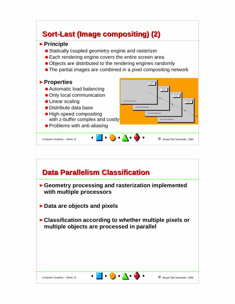
Sort-Last (Image compositing) (2)Sort-Last (Image compositing) (2)

GeometryEngine


GeometryEngine


GeometryEngine


GeometryEngine


PrincipleStatically coupled geometry engine and rasterizerEach rendering engine covers the entire screen areaObjects are distributed to the rendering engines randomlyThe partial images are combined in a pixel compositing network

PropertiesAutomatic load balancingOnly local communicationLinear scalingDistribute data baseHigh-speed compositing with z-buffer complex and costlyProblems with anti-aliasing


Data Parallelism ClassificationData Parallelism Classification

Geometry processing and rasterization implemented with multiple processors

Data are objects and pixels

Classification according to whether multiple pixels or multiple objects are processed in parallel


Image-space ParallelismImage-space Parallelism

Pixels or screen regions are processed in parallel

Objects are processed sequentially

Pixel storage, i.e. frame buffer, is required since objects are processed in arbitrary order


Object-space ParallelismObject-space Parallelism

Primitives or groups of primitives (objects) are processed in parallel

Pixels are generated sequentially

Pixel storage, i.e. frame buffer, is not absolutely necessary because pixels can be generated in scan order.

However, is often included because processors cannot maintain perfect pixel synchronism.


Image vs. Object ParallelismImage vs. Object Parallelism

Properties Image Space Object SpaceScreen resolution More processors Faster processorsPixel throughput More processors Faster processorsObject throughput Faster processors More processorsNumber of objects Faster processors More processorsMax number of processors Number of pixels Number of objects

Primitive types Fixed, all processors handle the same type

Configurable, new processor for new

primitive type


Summary: Graphics HardwareSummary: Graphics Hardware

Structure of display devices: CRT and LCD

Basics of graphics architectures

Screen refresh and frame buffer access problem

Performance modeling and bandwidth issues

Basics of parallel graphics architectures


Further ReadingFurther Reading

Displays:D. Bosman, Display Engineering, North Holland, 1989

Frame Buffer IssuesMary C. Whitton, Memory Design for Raster Graphics Displays, IEEE Computer Graphics & Applications, March 1984


ColorColor


ColorColor

Color SpecificationPerceptualPhysical and PsychophysicalColor Spaces


Perceptual Color Specification (1)Perceptual Color Specification (1)Color based on perception typically distinguishes between 3 components

Hue Based on the dominant wavelengthThe "actual" color, e.g. red, yellow, brown

LightnessThe (achromatic) intensity of the color

Brightness: For luminous objects (light emitter), e.g. CRTBrightness: For luminous objects (light emitter), e.g. CRTLightness: For reflecting objects, e.g. paper, wood.Lightness: For reflecting objects, e.g. paper, wood.

SaturationDistance of the color from a gray of equal intensitySaturated are more brilliant than unsaturated colorsUnsaturated color contain more white, e.g. pastels


Perceptual Color Specification (2)Perceptual Color Specification (2)

Black

White PureRed

Shades

Grays

Tones

Tints

Artists often use slightly different terms:

Pure PigmentsSaturated colorsSaturated colors

TintsAdd white pigments to pure colorAdd white pigments to pure colorReduces saturationReduces saturationIncrease lightnessIncrease lightness

ShadesAdd black pigments to pure colorAdd black pigments to pure colorReduces lightness and saturationReduces lightness and saturation

TonesAdd black and white pigments Add black and white pigments


Perceptual Color Specification (3)Perceptual Color Specification (3)

Textual SpecificationMix of pure colors, e.g. "Yellowish Green"Shades of pure colors, e.g. "Dark Blue"In reference to shared (?) perception, e.g. "Dusty Blue"

By Reference to SamplesOften used in printing, graphic design and interior design (paint chips), e.g. Munsell color-order systemFairly elaborate color catalogs

All perceptual color specifications are subjectiveDiffer between observersColor impression depends on lighting and surrounding colors


Physical Color Specification (1)Physical Color Specification (1)

ColorimetryColor is described by a spectrum

Spectral energy distribution P(λ) determines the colorSame perceived color can be created by several spectra called metamers

Spectra are continuous or discrete

Only one spectral line, are called monochromaticConstant energy across the entire spectrum: achromatic

P( )λ

λ400 nm 700 nm


Physical Color Specification (2)Physical Color Specification (2)

Color in physical terms is defined byDominant wavelengthExcitation purityLuminance

There is loose relationship between the terms used in both specification systems:

Perceptual ColorimetryHue Dominant Wavelength

Saturation Excitation PurityLightness LuminanceBrightness Luminance


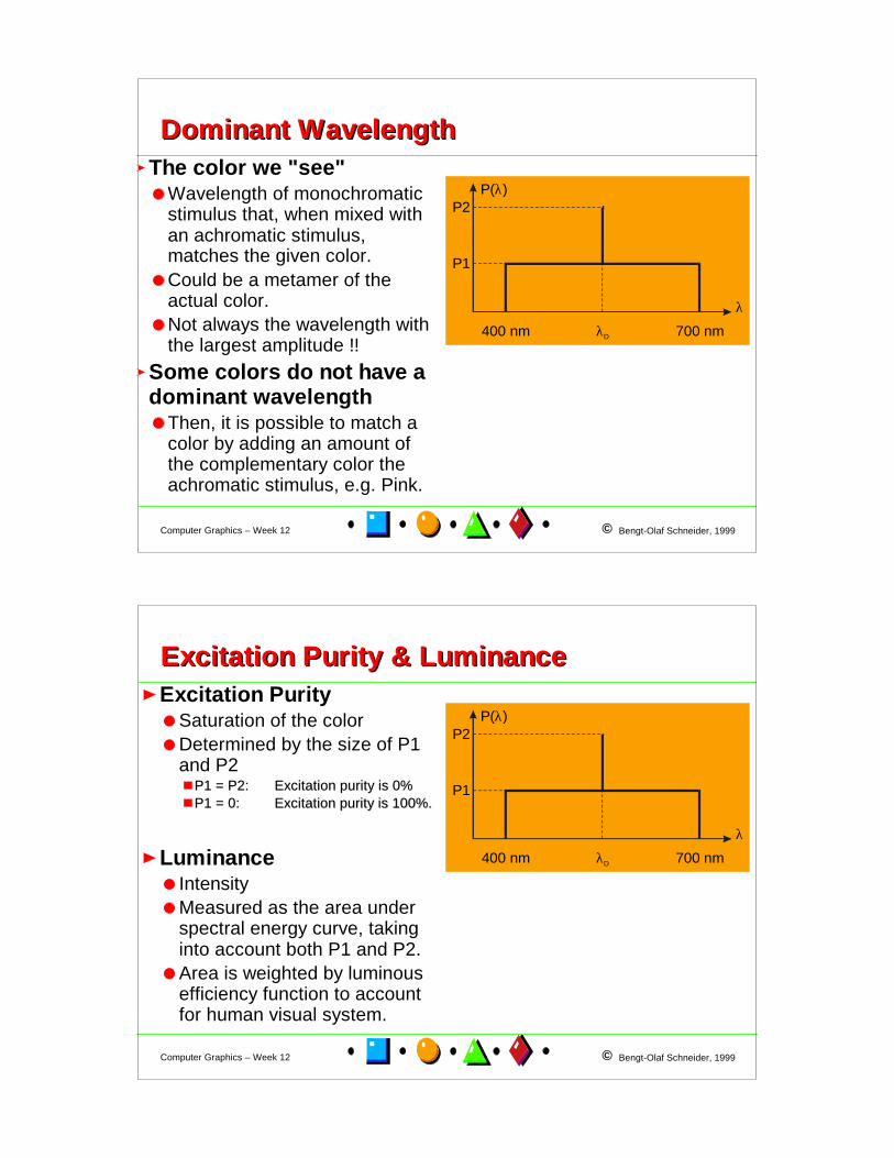
Dominant WavelengthDominant WavelengthThe color we "see"

Wavelength of monochromatic stimulus that, when mixed with an achromatic stimulus, matches the given color.Could be a metamer of the actual color.Not always the wavelength with the largest amplitude !!

Some colors do not have a dominant wavelength

Then, it is possible to match a color by adding an amount of the complementary color the achromatic stimulus, e.g. Pink.

P( )λ

λλD400 nm

P2

P1

700 nm


Excitation Purity & LuminanceExcitation Purity & LuminanceExcitation Purity

Saturation of the colorDetermined by the size of P1 and P2

P1 = P2:P1 = P2: Excitation purity is 0%Excitation purity is 0%P1 = 0:P1 = 0: Excitation purity is 100%.Excitation purity is 100%.

LuminanceIntensityMeasured as the area under spectral energy curve, taking into account both P1 and P2.Area is weighted by luminous efficiency function to account for human visual system.

P( )λ

λλD400 nm

P2

P1

700 nm


Luminous EfficiencyLuminous EfficiencyPerceived brightness for light of constant luminance

Sensitivity of the human visual system to different wavelengthsPeak sensitivity at 555 nm (yellow-green)Experimentally: Sum of the spectral response functions of cones

400 420 440 460 480 500 520 540 560 580 600 620 640 660 680 700

Wavelength [nm]

0

0.2

0.4

0.6

0.8

1

Rel

ativ

e S

ensi

tivity

Data from Wyszecki & Stiles, 1982.


Spectral Response of Cones (1)Spectral Response of Cones (1)

400

420

440

460

480

500

520

540

560

580

600

620

640

660

680

700

Wavelength

0

0.1

0.2

0.3

0.4

0.5

0.6

0.7

Abs

orpt

ion

0

0.2

0.4

0.6

0.8

1

1.2

1.4


Sum of the absorption curves.(approx. luminous efficiency)



400

420

440

460

480

500

520

540

560

580

600

620

640

660

680

700

Wavelength

0

0.1

0.2

0.3

0.4

0.5

0.6

0.7

Abs

orpt

ion


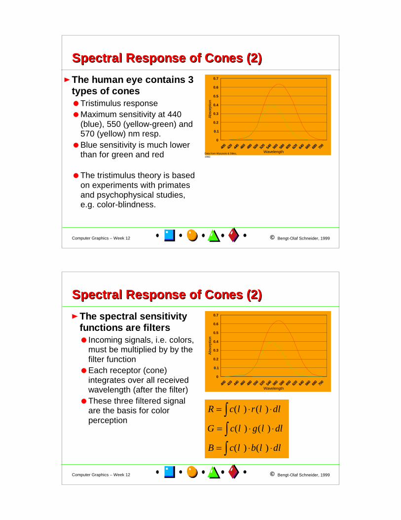
The human eye contains 3 types of cones

Tristimulus responseMaximum sensitivity at 440 (blue), 550 (yellow-green) and 570 (yellow) nm resp.Blue sensitivity is much lower than for green and red

The tristimulus theory is based on experiments with primates and psychophysical studies, e.g. color-blindness.



400

420

440

460

480

500

520

540

560

580

600

620

640

660

680

700

Wavelength

0

0.1

0.2

0.3

0.4

0.5

0.6

0.7

Abs

orpt

ion

The spectral sensitivity functions are filters

Incoming signals, i.e. colors, must be multiplied by by the filter functionEach receptor (cone) integrates over all received wavelength (after the filter)These three filtered signal are the basis for color perception

R c r d

G c g d

B c b d

= ◊ ◊

= ◊ ◊

= ◊ ◊

zzz

( ) ( )

( ) ( )

( ) ( )

λ λ λ

λ λ λ

λ λ λ


MetamersMetamers

The tristimulus theory provides an explanation of metamers

Spectra that create the same signals in the photorecptors are perceived as the same color, although the spectra may differ !

Monochromatic (spectral) lights create unique responses. Therefore, two spectral colors cannot be metamers for each other.

Note: Metamers are a solely perceptual effect. Instruments can distinguish between metameric lights.


Color MixingColor Mixing

Tristimulus theory suggests that all colors can be created by stimulating the three types of cones to different extents.

This is the principle of additive and subtractive color mixing


Tristimulus Color MatchingTristimulus Color MatchingTristimulus theory suggests that all colors can be created by stimulating the three types of cones to different extents.

Many colors (e.g. CRT) can be generated that way ... but not all !

Color Matching ExperimentSynthesize a sample color by additive mixing of 3 spectral colors

Blue: 435.8 nm, Green: 546.1, Red: 700 nmBlue: 435.8 nm, Green: 546.1, Red: 700 nmRelative radiant power B:G:R = 72.1 : 1.4 : 1.0Relative radiant power B:G:R = 72.1 : 1.4 : 1.0

Luminance for each color can be adjusted between -1 and +1Luminance <0 means adding it to the sampleFor a few colors, Red must be subtracted to match the sample color, i.e. Red had to be added to the color sample.The experiment results in a set of wavelength-dependent color matching functions needed to match all monochromatic colors.


Tristimulus Color Matching Functions (1)Tristimulus Color Matching Functions (1)

380

400

420

440

460

480

500

520

540

560

580

600

620

640

660

680

700

720

740

760

780

Wavelength [nm]

-0.1

0

0.1

0.2

0.3

0.4

Tris

timul

us V

alue

s

435.8 nm 546.1 nm 700.0 nm

b ( )λ

g ( )λ

r ( )λ


Tristimulus Color Matching Functions (2)Tristimulus Color Matching Functions (2)

These functions can be normalized so that only 2 of the 3 functions are independent

One can be computed given the two other functionsTypically, r(λ) and g(λ) are chosen as the independent functionsPlotting the two independent matching functions creates (r,g)-Chromaticity Diagram

rr

r g b

gg

r g b

bb

r g b

( )( )

( ) ( ) ( )

( )( )

( ) ( ) ( )

( )( )

( ) ( ) ( )

λ λλ λ λ

λ λλ λ λ

λ λλ λ λ

= + +

= + +

= + +

r g b

b r g

( ) ( ) ( )

( ) ( ) ( )

λ λ λ

λ λ λ

+ + =fi

= - -

1

1


Tristimulus Tristimulus (r,g)(r,g)-Chromaticity Diagram-Chromaticity Diagram

-1.5 -1 -0.5 0 0.5 1

Red

0

0.5

1

1.5

2

Gre

en

380 nm

550 nm

540 nm

530 nm

520 nm

470 nm

480 nm

490 nm

500 nm

510 nm

570 nm560 nm

580 nm

700 nm

bluered

green

purple line


CIE Color Matching Functions (1)CIE Color Matching Functions (1)

The negative contributions from the tristimulus color matching functions are inconvenient and non-intuitiveCIE color matching functions have only positive weights

CIE = Commission Internationale de l'EclairageDifferent primaries X, Y and Z that replace R, G, and BCorresponding color matching functions x'(λ), y'(λ), z'(λ).The primary Y was chosen, so that the color matching function y'(λ) is identical to the luminous efficiency function.

Note, that x'(λ), y'(λ), z'(λ) are not spectral distribution of the primary colors X, Y, Z.They simply functions that indicate how much of X, Y, Z is needed to match a sample color.


380

400

420

440

460

480

500

520

540

560

580

600

620

640

660

680

700

720

740

760

780

Wavelength [nm]

0

0.5

1

1.5

2

Tris

timul

us V

alue

x' y' z'




For a given spectral distribution P(λ), we compute the weights X, Y, Z for each of the matching functions as:

For self-luminous objects: k=680 lm/WFor reflecting objects, k is chosen such that a bright white gives Y=100, i.e.

Then each color C is described as

X k P x d Y k P y d Z k P z d= ◊ ◊ = ◊ ◊ = ◊ ◊z z z( ) ( ) ( ) ( ) ( ) ( )λ λ λ λ λ λ λ λ λ

kP y dW

=◊ ◊z

100( ) ( )λ λ λ

C X Y Z= ◊ + ◊ + ◊X Y Z



The colors C are contained in the space defined by all valid values of X, Y, Z.

Y

Z

X



Similar to the tristimulus color matching functions, the CIE functions can be normalized

xx

x y z

yy

x y z

zz

x y z

( )( )

( ) ( ) ( )

( )( )

( ) ( ) ( )

( )( )

( ) ( ) ( )

λ λλ λ λ

λ λλ λ λ

λ λλ λ λ

= + +

= + +

= + +

x y z( ) ( ) ( )λ λ λ+ + = 1


CIE Chromaticity Diagram (1)CIE Chromaticity Diagram (1)

The CIE chromaticity diagram is the projection of the plane X+Y+Z=1 onto the XY-plane.

Monochromatic colors along the borderUnsaturated colors in the interiorSeveral white points defined

Equal energy, x = y = z = 1/3Equal energy, x = y = z = 1/3SunlightSunlightDifferent "white" lightsDifferent "white" lights


CIE Chromaticity Diagram (2)CIE Chromaticity Diagram (2)Chromaticity diagram only contains dominant wavelenth and excitation purityLuminance information is excluded:

Given two values, e.g. x and y, we can recover the third (here z):

However, the original values X, Y and Z cannot be recoverd !This requires one of the original values, e.g. Y. Then we get:

Remember: The chromaticity contains all visibile colors of a given luminance ... not simply all visible colors !

x y z( ) ( ) ( )λ λ λ+ + = 1

X Yxy

Y Y Z Yx yy

= = = - -

1


Using the CIE Chromaticity Diagram (1)Using the CIE Chromaticity Diagram (1)

Dominant wavelenthDraw line from the white point W to the color C and continue to the intersection point C' with the border of the chromaticity diagram.The intersection point is the dominant wavelenth.Here: approx. 565 nm

Excitation purityThe ratio of the WC / WC' is the excitation purity.Here: approx. 50%

W

C'

C



Mixing ColorsAll colors along a line in the chromaticity diagram can be created by mixing the colors at the endpoints, e.g. Similarly, all colors in a convex polygon can be created by mixing the colors a the vertices.

A

B

C



W

C'

C

Complementary ColorsMixing complementary colors produces white light.C and C' are complementary colors as the midpoint of their connecting line passes through the white point.

Note: White can be produced by either 2 colors or by a constant spectrum (also see additive color mixing).


Using the CIE Chromaticity Diagram (4)Using the CIE Chromaticity Diagram (4)Non-spectral Colors

Some colors do not have dominant wavelengthAll colors that lie on a line from the white point towards the purple lineComplement of a spectral color (i.e. color with a dominant wavelength).Excitation purity is defined as before.

Here:C is the complementary color of C' at approx. 505 nm.

W

C'

C


Color DistancesColor Distances

Colors that visually differ by the same amount appear at different distances in the CIE chromaticity diagram

Another CIE diagram, the CIE LUV defines a uniform color spaceMore intuitive prediction of color difference from color coordinates.


The CIE chromaticity diagram can describe all visible colors (given a luminance)

Therefore, it can be used to define, name and compare colors

We will use the CIE color specification to analyze other color specification schemes

Such specifications define a gamut in the space of visible color

Most gamuts specify colors by mixing several primaries and can therefore not represent all visible colors

Remember: Negative contributions are required to produce all colors !Remember: Negative contributions are required to produce all colors !

Color Gamuts (1)Color Gamuts (1)


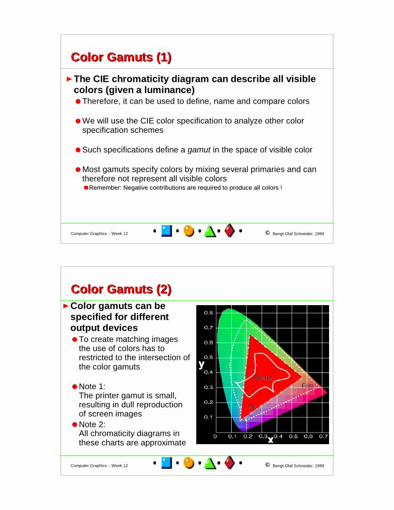
Color Gamuts (2)Color Gamuts (2)Color gamuts can be specified for different output devices

To create matching images the use of colors has to restricted to the intersection of the color gamuts

Note 1: The printer gamut is small, resulting in dull reproduction of screen images Note 2:All chromaticity diagrams in these charts are approximate

FilmFilm

TVTV

PrinterPrinter


Summary: Color SpecificationSummary: Color Specification

Perceptual and Physical Color DefinitionCorrespondence between terms

Linear combinations of primary colors can not produce all visible colors

Established using color matching experimentsDue to non-linearities of the human visual system

CIE Chromaticity DiagramUses matching functions that are non-negative for all wavelengthsCan be used to define colors and evaluate color models


Further ReadingFurther Reading

For Color Science:Guenther Wyszecki, W.S. Stiles, "Color Science: Concepts and Methods, Quantitative Data and Formulae", 2nd edition, John Wiley & Sons, 1982.

For YIQ Color Model: Keith Jack, "Video Demystified", HighText Publications, 1993.


HomeworkHomework

Review graphics hardware and color theory

Prepare volume rendering (chapter 20.6)

Review entire class material


Next Week ...Next Week ...

Conclusion of color theoryColor modelsUse of color

Volume Rendering

Q + A

Green

Blue

Yellow(-B)

Magenta(-G)

BlackCyan(-R)

Red

Computer Graphics - Week 12 - Department of …feiner/courses/csw4160/slides/S99-12.pdfComputer...

Documents

Transcript of Computer Graphics - Week 12 - Department of …feiner/courses/csw4160/slides/S99-12.pdfComputer...