Computer AnimationNadia Magnenat ThalmannMIRALab, University of Geneva

Geneva, SwitzerlandE-mail: thalmann@cui.unige.ch

Daniel ThalmannComputer Graphics Lab

Swiss Federal Institute of Technology (EPFL)Lausanne, Switzerland

E-mail: thalmann@lig.di.epfl.ch

IntroductionThe main goal of computer animation is to synthesize the desired motion effect which is a mixing of

natural phenomena, perception and imagination. The animator designs the object's dynamic

behavior with his mental representation of causality. He/she imagines how it moves, gets out of shape

or reacts when it is pushed, pressed, pulled, or twisted. So, the animation system has to provide the

user with motion control tools able to translate his/her wishes from his/her own language. Computer

animation methods may also help to understand physical laws by adding motion control to data in

order to show their evolution over time. Visualization has become an important way of validating

new models created by scientists. When the model evolves over time, computer simulation is

generally used to obtain the evolution of time, and computer animation is a natural way of

visualizing the results obtained from the simulation.

To produce a computer animation sequence, the animator has two principal techniques available.

The first is to use a model that creates the desired effect. A good example is the growth of a green

plant. The second is used when no model is available. In this case, the animator produces "by hand"

the real world motion to be simulated. Until recently most computer-generated films have been

produced using the second approach: traditional computer animation techniques like keyframe

animation, spline interpolation, etc. Then, animation languages, scripted systems and director-

oriented systems were developed. In the next generation of animation systems, motion control tends

to be performed automatically using A.I. and robotics techniques. In particular, motion is planned at

a task level and computed using physical laws. More recently, researchers have developed models of

behavioral animation and simulation of autonomous creatures.

2

State variables and evolution laws

Computer animation may be defined as a technique in which the illusion of movement is created by

displaying on a screen, or recording on a recording device a series of individual states of a dynamic

scene. Formally, any computer animation sequence may be defined as a set of objects characterized

by state variables evolving over time. For example, a human character is normally characterized

using its joint angles as state variables. To improve computer animation, attention needs to be

devoted to the design of evolution laws [Magnenat Thalmann and Thalmann, 1985]. Animators must

be able to apply any evolution law to the state variables which drive animation.

Classification of methods

Zeltzer [Zeltzer, 1985]classifies animation systems as being either guiding, animator-level or task-

level systems. In guiding systems, the behaviors of animated objects are explicitly described.

Historically, typical guiding systems were BBOP, TWIXT and MUTAN. In animator level systems, the

behaviors of animated objects are algorithmically specified. Typical systems are: GRAMPS, ASAS

and MIRA. More details on these systems may be found in [Magnenat Thalmann and Thalmann,

1990]. In task level systems, the behaviors of animated objects are specified in terms of events and

relationships. There is no general-purpose task-level system available now, but it should be

mentioned that JACK [Badler et al., 1993] and HUMANOID [Boulic et al., 1995] are steps towards

task-level animation.

Magnenat Thalmann and Thalmann [1991] propose a new classification of computer animation

scenes involving synthetic actors both according to the method of controlling motion and according

to the kinds of interactions the actors have. A motion control method specifies how an actor is

animated and may be characterized according to the type of information to which it is privileged in

animating the synthetic actor. For example, in a keyframe system for an articulated body, the

privileged information to be manipulated is joint angles. In a forward dynamics-based system, the

privileged information is a set of forces and torques; of course, in solving the dynamic equations,

joint angles are also obtained in this system, but we consider these as derived information. In fact,

any motion control method will eventually have to deal with geometric information (typically joint

angles), but only geometric motion control methods are explicitly privileged to this information at

the level of animation control.

3

The nature of privileged information for the motion control of actors falls into three categories:

geometric, physical and behavioral, giving rise to three corresponding categories of motion control

method.

• The first approach corresponds to methods heavily relied upon by the animator: performance

animation, shape transformation, parametric keyframe animation. Animated objects are

locally controlled. Methods are normally driven by geometric data. Typically the animator

provides a lot of geometric data corresponding to a local definition of the motion.

• The second way guarantees a realistic motion by using physical laws, especially dynamic

simulation. The problem with this type of animation is controlling the motion produced by

simulating the physical laws which govern motion in the real world. The animator should

provide physical data corresponding to the complete definition of a motion. The motion is

obtained by the dynamic equations of motion relating the forces, torques, constraints and the

mass distribution of objects. As trajectories and velocities are obtained by solving the equations,

we may consider actor motions as globally controlled. Functional methods based on

biomechanics are also part of this class.

• The third type of animation is called behavioral animation and takes into account the

relationship between each object and the other objects. Moreover the control of animation may

be performed at a task level, but we may aso consider the animated objects as autonomous

creatures. In fact, we will consider as a behavioral motion control method any method which

drives the behavior of objects by providing high-level directives indicating a specific behavior

without any other stimulus.

Underlying Principles and Best Practices

Geometric and Kinematics Methods

IntroductionIn this group of methods, the privileged information is of a geometric or kinematics nature.

Typically, motion is defined in terms of coordinates, angles and other shape characteristics or it may

be specified using velocities and accelerations, but no force is involved. Among the techniques based

4

on geometry and kinematics, we will discuss performance animation, keyframing, morphing, inverse

kinematics and procedural animation. Although these methods have been mainly concerned with

determining the displacement of objects, they may also be applied in calculating deformations of

objects.

Motion Capture and Performance Animation

Performance animation or motion capture consist of measurement and recording of direct actions of

a real person or animal for immediate or delayed analysis and playback. The technique is especially

used today in production environments for 3D character animation. It involves mapping of

measurements onto the motion of the digital character. This mapping can be direct: e.g. human arm

motion controlling a character's arm motion or indirect: e.g. mouse movement controlling a

character's eye and head direction. Maiocchi [1995] gives more details about performance

animation.

We may distinguish three kinds of systems: mechanical, magnetic, and optical.

Mechanical systems or digital puppetry allows animation of 3D characters through the use of any

number of real-time input devices: mouse, joysticks, datagloves, keyboard, dial boxes. The

information provided by manipulation of such devices is used to control the variation of parameters

over time for every animating feature of the character.

Optical motion capture systems are based on small reflective sensors called markers attached to an

actor's body and on several cameras focused on performance space. By tracking positions of

markers, one can get locations for corresponding key points in the animated model, e.g. we attach

markers at joints of a person and record the position of markers from several different directions.

We then reconstruct the 3D position of each key point at each time. The main advantage of this

method is freedom of movement; it does not require any cabling. There is however one main

problem: occlusion. i.e., lack of data resulting from hidden markers for example when the

performer lies on his back. Another problem comes with the lack of an automatic way of

distinguishing reflectors when they get very close to each other during motion. These problems may

be minimized by adding more cameras, but at a higher cost, of course. Most optical systems operate

with four or six cameras. Good examples of optical systems are the ELITE and the VICON systems.

5

Magnetic motion capture systems require the real actor to wear a set of sensors, which are capable of

measuring their spatial relationship to a centrally located magnetic transmitter. The position and

orientation of each sensor is then used to drive an animated character. One problem is the need for

synchronizing receivers. The data stream from the receivers to a host computer consists of 3D

positions and orientations for each receiver. For human body motion, eleven sensors are generally

needed: one on the head, one on each upper arm, one on each hand, one in the center of chest, one

on the lower back, one on each ankle, and one on each foot. To calculate the rest of the necessary

information, the most common way is the use of inverse kinematics. The two most popular magnetic

systems are: Polhemus Fastrack and Ascension Flock of Birds.

Motion capture methods offer advantages and disadvantages. Let us consider the case of human

walking. A walking motion may be recorded and then applied to a computer-generated 3D

character. It will provide a very good motion, because it comes directly from reality. However,

motion capture does not bring any really new concept to animation methodology. For any new

motion, it is necessary to record the reality again. Moreover, motion capture is not appropriate

especially in real-time simulation activities, where the situation and actions of people cannot be

predicted ahead of time, and in dangerous situations, where one cannot involve a human actor.

VR-based animation

When motion capture is used on line, it is possible to create applications based on a full 3-D

interaction metaphor in which the specifications of deformations or motion are given in real-time.

This new concept drastically changes the way of designing animation sequences. Thalmann [1993]

calls all techniques based on this new way of specifying animation VR-based animation techniques.

He also calls VR devices all interactive devices allowing to communicate with virtual worlds. They

include classic devices like head-mounted display systems, DataGloves as well as all 3D mice or

SpaceBalls. He also considers as VR devices MIDI keyboards, force-feedback devices and

multimedia capabilities like real-time video input devices and even audio input devices. During the

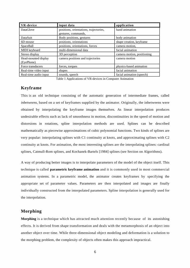
animation creation process, the animator should enter a lot of data into the computer. Table 1 shows

VR devices and the corresponding data and applications.

6

VR-device input data applicationDataGlove positions, orientations, trajectories,

gestures, commands,hand animation

DataSuit Body positions, gestures body animation6D mouse positions, orientations shape creation, keyframeSpaceBall positions, orientations, forces camera motion,MIDI keyboard multi-dimensional data facial animationStereo display 3D perception camera motion, positioningHead-mounted display(EyePhone)

camera positions and trajectories camera motion

Force transducers forces, torques physics-based animationReal-time video input shapes facial animationReal-time audio input sounds, speech facial animation (speech)

Table 1 Applications of VR-devices in Computer Animation

Keyframe

This is an old technique consisting of the automatic generation of intermediate frames, called

inbetweens, based on a set of keyframes supplied by the animator. Originally, the inbetweens were

obtained by interpolating the keyframe images themselves. As linear interpolation produces

undesirable effects such as lack of smoothness in motion, discontinuities in the speed of motion and

distorsions in rotations, spline interpolation methods are used. Splines can be described

mathematically as piecewise approximations of cubic polynomial functions. Two kinds of splines are

very popular: interpolating splines with C1 continuity at knots, and approximating splines with C2

continuity at knots. For animation, the most interesting splines are the interpolating splines: cardinal

splines, Catmull-Rom splines, and Kochanek-Bartels [1984] splines (see Section on Algorithms).

A way of producing better images is to interpolate parameters of the model of the object itself. This

technique is called parametric keyframe animation and it is commonly used in most commercial

animation systems. In a parametric model, the animator creates keyframes by specifying the

appropriate set of parameter values. Parameters are then interpolated and images are finally

individually constructed from the interpolated parameters. Spline interpolation is generally used for

the interpolation.

Morphing

Morphing is a technique which has attracted much attention recently because of its astonishing

effects. It is derived from shape transformation and deals with the metamorphosis of an object into

another object over time. While three-dimensional object modeling and deformation is a solution to

the morphing problem, the complexity of objects often makes this approach impractical.

7

The difficulty of the three-dimensional approach can be effectively avoided with a two-dimensional

technique called image morphing. Image morphing manipulates two-dimensional images instead of

three-dimensional objects and generates a sequence of inbetween images from two images. Image

morphing techniques have been widely used for creating special effects in television commercials,

music videos, and movies.

The problem of image morphing is basically how an inbetween image is effectively generated from

two given images. A simple way for deriving an inbetween image is to interpolate the colors of each

pixel between two images. However, this method tends to wash away the features on the images and

does not give a realistic metamorphosis. Hence, any successful image morphing technique must

interpolate the features between two images to obtain a natural inbetween image.

Feature interpolation is performed by combining warps with the color interpolation. A warp is a two-

dimensional geometric transformation and generates a distorted image when it is applied to an

image. When two images are given, the features on the images and their correspondences are

specified by an animator with a set of points or line segments. Then, warps are computed to distort

the images so that the features have intermediate positions and shapes. The color interpolation

between the distorted images finally gives an inbetween image. More detailed processes for

obtaining an inbetween image are described by Wolberg [1990].

In generating an inbetween image, the most difficult part is to compute warps for distorting the given

images. Hence, the research in image morphing has concentrated on deriving warps from the

specified feature correspondence. Image morphing techniques can be classified into two categories

such as mesh-based and feature-based methods in terms of their ways for specifying features. In

mesh-based methods, the features on an image are specified by a nonuniform mesh. Feature-based

methods specify the features with a set of points or line segments. Lee and Shin [1995] has given a

good survey of digital warping and morphing techniques.

Inverse kinematics

This direct kinematics problem consists in finding the position of end point positions (e.g. hand,

foot) with respect to a fixed-reference coordinate system as a function of time without regard to the

forces or the moments that cause the motion. Efficient and numerically well-behaved methods exist

for the transformation of position and velocity from joint-space (joint angles) to Cartesian

8

coordinates (end of the limb). Parametric keyframe animation is a primitive application of direct

kinematics.

The use of inverse kinematics permits direct specification of end point positions. Joint angles are

automatically determined. This is the key problem, because independent variables in an articulated

system are joint angles. Unfortunately, the transformation of position from Cartesian to joint

coordinates generally does not have a closed-form solution. However, there are a number of special

arrangements of the joint axes for which closed-form solutions have been suggested in the context

of animation [Girard and Maciejewski, 1985]

Procedural Animation

Procedural animation corresponds to the creation of a motion by a procedure describing

specifically the motion. Procedural animation should be used when the motion can be described by

an algorithm or a formula. For example, consider the case of a clock based on the pendulum law:

α = A sin (ωt+φ)

A typical animation sequence may be produced using a program such as:

create CLOCK (...);for FRAME:=1 to NB_FRAMES

TIME:=TIME+1/24;ANGLE:=A*SIN (OMEGA*TIME+PHI);MODIFY (CLOCK, ANGLE);draw CLOCK;record CLOCKerase CLOCK

Procedural animation may be specified using a programming language or interactive system like the

Extensible Director-Oriented Systems MIRANIM [Magnenat Thalmann and Thalmann, 1990].

Character Deformations

Modeling and deformation of 3D characters and especially human bodies during the animation

process is an important but difficult problem. Researchers have devoted significant efforts to the

representation and deformation of the human body shape. Broadly, we can classify their models into

two categories: the surface model and the multi-layered model.

The surface model [Magnenat Thalmann and Thalmann, 1987] is conceptually simple, containing a

skeleton and outer skin layer. The envelope is composed of planar or curved patches. One problem

9

is that this model requires the tedious input of the significant points or vertices that define the

surface. Another main problem is that it is hard to control the realistic evolution of the surface across

joints. Surface singularities or anomalies can easily be produced. Simple observation of human skin

in motion reveals that the deformation of the outer skin envelope results from many other factors

besides the skeleton configuration.

The Multi-layered model [Chadwick et al., 1989] contains a skeleton layer, intermediate layers which

simulate the physical behavior of muscle, bone, fat tissue, etc., and a skin layer. Since the overall

appearance of a human body is very much influenced by its internal muscle structures, the layered

model is the most promising for realistic human animation. The key advantage of the layered

methodology is that once the layered character is constructed, only the underlying skeleton need be

scripted for an animation; consistent yet expressive shape deformations are generated automatically.

Jianhua and Thalmann [1995] describe a highly effective multi-layered approach for constructing

and animating realistic human bodies. Metaballs are employed to simulate the gross behavior of

bone, muscle, and fat tissue. They are attached to the proximal joints of the skeleton, arranged in an

anatomically-based approximation. The skin surfaces are automatically constructed using cross-

sectional sampling. Their method, simple and intuitive, combines the advantages of implicit,

parametric and polygonal surface representation, producing very realistic and robust body

deformations. By applying smooth blending twice (metaball potential field blending and B-spline

basis blending), the data size of the model is significantly reduced.

Physics-based methods

Dynamic Simulation

Kinematics-based systems are generally intuitive but lack dynamic integrity. The animation does not

seem to respond to basic physical facts like gravity or inertia. Only modeling of objects that move

under the influence of forces and torques can be realistic. Methods based on parameter adjustment

are the most popular approach to dynamics-based animation and correspond to non-constraint

methods. There is an alternative: the constraint-based methods: the animator states in terms of

constraints the properties the model is supposed to have, without needing to adjust parameters to give

it those properties. In dynamic-based simulation, there are also two problems to be considered: the

forward dynamics problem and the inverse-dynamics problem. The forward dynamics problem

10

consists of finding the trajectories of some point (e.g. an end effector in an articulated figure) with

regard to the forces and torques that cause the motion. The inverse-dynamics problem is much more

useful and may be stated as follows: determine the forces and torques required to produce a

prescribed motion in a system. Non-constraint methods have been mainly used for the animation of

articulated figures [Armstrong et al., 1987]. There are a number of equivalent formulations which

use various motion equations: Newton–Euler formulation (see Section on algorithms), Lagrange

formulation, Gibbs–Appell formulation, D'Alembert formulation. These formulations are popular in

robotics and more details about the equations and their use in computer animation may be found in

[Thalmann, 1990]. Fig.1 shows an example of animation based on dynamics.

Fig. 1. A motion calculated using dynamic simulation

Concerning Constraint-based Methods, Witkin and Kass [1988] propose a new method, called

Spacetime Constraints, for creating character animation. In this new approach, the character motion

is created automatically by specifying what the character has to be, how the motion should be

performed, what the character's physical structure is, and what physical resources are available to the

character to accomplish the motion. The problem to solve is a problem of constrained optimization.

Cohen [1992] takes this concept further and uses a subdivision of spacetime into discrete pieces, or

11

Spacetime Windows, over which subproblems can be formulated and solved. The sensitivity of

highly non-linear constrained optimization to starting values and solution algorithms can thus be

controlled to a great extent by the user.

Physics-based Deformations

Physics-based models

Realistic simulation of deformations may be only performed using physics-based animation. The

most well-known model is the Terzopoulos elastic model [Terzopoulos et al., 1987]. In this model,

the fundamental equation of motion corresponds to an equilibrium between internal forces (inertia,

resistance to stretching, dissipative force, resistance to bending) and external forces (e.g. collision

forces, gravity, seaming and attaching forces, wind force). Gourret et al. [1989] propose a finite

element method to model the deformations of human flesh due to flexion of members and/or

contact with objects. The method is able to deal with penetrating impacts and true contacts.

Simulation of impact with penetration can be used to model the grasping of ductile objects, and

requires decomposition of objects into small geometrically simple objects. All the advantages of

physical modeling of objects can also be transferred to human flesh. For example, the hand grasp of

an object is expected to lead to realistic flesh deformation as well as an exchange of information

between the object and the hand which will not only be geometrical.

Collision Detection and ResponseIn computer animation, collision detection and response are obviously more important. Some works

have addressed collision detection and response. Hahn [1988] presented bodies in resting contact as

a series of frequently occurring collisions. Baraff [1989]presented an analytical method for finding

forces between contacting polyhedral bodies, based on linear programming techniques. He also

proposed a formulation of the contact forces between curved surfaces that are completely

unconstrained in their tangential movement. Bandi et al. [1995] introduced an adaptive spatial

subdivision of the object space based on octree structure and presented a technique for efficiently

updating this structure periodically during the simulation. Volino and Magnenat Thalmann

[1994]described a new algorithm for detecting self-collisions on highly discretized moving

polygonal surfaces. It is based on geometrical shape regularity properties that permit avoiding many

useless collision tests.

12

A case study: Cloth Animation

Weil [Weil, 1986] pioneered cloth animation using an approximated model based on relaxation of

the surface. Kunii and Godota [1990] used a hybrid model incorporating physical and geometrical

techniques to model garment wrinkles. Aono [ 1990] simulated wrinkle propagation on a

handkerchief using an elastic model. Terzopoulos et al. applied their general elastic to a wide range

of objects including cloth. Lafleur et al. [1991] and Carignan et al. [1992] have described complex

interaction of clothes with synthetic actors in motion, which marked the beginning of a new era in

cloth animation. However, there were still a number of restrictions on the simulation conditions on

the geometrical structure and the mechanical situations, imposed by the simulation model or the

collision detection. More recently, Volino et al. [1995] propose a mechanical model to deal with any

irregular triangular meshes, handle high deformations despite rough discretisation, and cope with

complex interacting collisions. Fig.2 shows an example of cloth animation.

Fig. 2. Cloth animation

13

Behavioral methods

Task-level Animation

Similarly to a task-level robotic system, actions in a task level animation system are specified only by

their effects on objects. Task-level commands are transformed into low-level instructions such as a

script for algorithmic animation or key values in a parametric keyframe approach. Typical

examples of tasks for synthetic actors are:

• walking from an arbitrary point A to another point B• pick up an object at location A and move it to location B• speak a sentence or make a high-level expression

Similarly to robotics systems, we may divide task planning for synthetic actors into three phases:

world modelling, task specification and code generation.

The Grasping Task

In the computer animation field, interest in human grasping appeared with the introduction of the

synthetic actors. Magnenat Thalmann et al. [1988] describe one of the first attempts to facilitate the

task of animating actors' interaction with their environment. However, the animator has to position

the hand and decide the contact points of the hand with the object. Rijpkema and Girard [1991]

presents a full description of a grasping system that allows both, an automatic or an animator chosen

grasp. The main idea is to approximate the objects with simple primitives. The mechanisms to grasp

the primitives are known in advance and constitute what they call the knowledge database. Recently,

Mas and Thalmann [1994] have presented a hand control and automatic grasping system using an

inverse kinematics based method. In particular, their system can decide to use a pinch when the

object is too small to be grasped by more than two fingers or to use a two-handed grasp when the

object is too large.

Fig.3 shows an example of object grasping scene.

14

Fig. 3. Object grasping scene

The Walking Task

Zeltzer [1982] describes a walk controller invoking 12 local motor programs to control the actions

of the legs and the swinging of the arms. Bruderlin and Calvert [Bruderlin and Calvert, 1989]

propose a hybrid approach to the human locomotion which combines goal-oriented and dynamic

motion control. Knowledge about a locomotion cycle is incorporated into a hierarchical control

process. Decomposition of the locomotion determines forces and torques that drive the dynamic

model of the legs by numerical approximation techniques. McKenna and Zeltzer [1990] describe an

efficient forward dynamic simulation algorithm for articulated figures which has a computational

complexity linear in the number of joints. Boulic et al. [1990] propose a model built from

experimental data based on a wide range of normalized velocities. At a first level, global spatial and

temporal characteristics (normalized length and step duration) are generated. At the second level, a

set of parameterized trajectories produce both the position of the body in the space and the internal

body configuration. The model is designed to keep the intrinsic dynamic characteristics of the

15

experimental model. Such an approach also allows a personification of the walking action in an

interactive real-time context in most cases. Fig.4. shows an example walking sequence.

Fig. 4. Walking sequence

Artificial and Virtual Life

This kind of research is strongly related to the research efforts in behavioral animation introduced

by Reynolds [1987] study in his distributed behavioral model simulating flocks of birds, herds of

land animals and fish schools. For birds, the simulated flock is an elaboration of a particle system

with the simulated birds being the particles. A flock is assumed to be the result of the interaction

between the behaviors of individual birds. Working independently, the birds try both to stick

together and avoid collisions with one another and with other objects in their environment. In a

module of behavioral animation, positions, velocities and orientations of the actors are known from

the system at any time. The animator may control several global parameters: e.g. weight of the

obstacle avoidance component, weight of the convergence to the goal, weight of the centering of the

group, maximum velocity, maximum acceleration, minimum distance between actors. The animator

provides data about the leader trajectory and the behavior of other birds relatively to the leader. The

computer-generated film Stanley and Stella was produced using this distributed behavioral model.

Wilhelms [Wilhelms] proposes a system based on a network of sensors and effectors. Ridsdale [1990]

16

proposes a method that guides lower-level motor skills from a connectionist model of skill memory,

implemented as collections of trained neural networks. We should also mention the huge literature

about autonomous agents which represents a background theory for behavioral animation. More

recently, genetic algorithms were also proposed to automatically generate morphologies for artificial

creatures and the neural systems for controlling their muscle forces.

L-system-based behavioral animation

Another approach for behavioral animation is based on timed and parameterized L-systems [Noser

et al., 1992] with conditional and pseudo stochastic productions. With this production-based

approach a user may create any realistic or abstract shape, play with fascinating tree structures and

generate any concept of growth and life development in the resulting animation. To extend the

possibilities for more realism in the pictures, external forces have been added, which interact with the

L-structures and allow a certain physical modeling. External forces can also have an important

impact in the evolution of objects. Tree structures can be elastically deformed and animated by time

and place dependent vector force fields. The elasticity of each articulation can be set individually by

productions. So, the bending of branches can be made dependent on the branches' thickness,

making animation more realistic. The force fields too, can be set and modified with productions.

Force can directly affect L-structures. It is possible to simulate the displacement of objects in any

vector force field dependent on time and position. An object movement is determined by a class of

differential equations, which can be set and modified by productions. The mass of the turtle, who

represents the object, can be set as well, by using a special symbol of the grammar. This vector force

field approach is particularly convenient to simulate the motion of objects in fluids (air, water).

Virtual Sensors

Perception through Virtual Sensors

In a typical behavioral animation scene , the actor perceives the objects and the other actors in the

environment, which provides information on their nature and position. This information is used by

the behavioral model to decide the action to take, which results in a motion procedure. In order to

implement perception, virtual humans should be equipped with visual, tactile and auditory sensors.

These virtual sensors should be used as a basis for implementing everyday human behaviour such

as visually directed locomotion, handling objects, and responding to sounds and utterances. For

17

synthetic audition [Noser and Thalmann, 1995], one needs to model a sound environment where the

synthetic actor can directly access positional and semantic sound source information of audible

sound events. Simulating the haptic system corresponds roughly to a collision detection process. But,

the most important perceptual subsystem is the vision system as described in the next section.

Virtual vision

The concept of synthetic vision was first introduced by Renault et al. [1990] as a main information

channel between the environment and the virtual actor. Reynolds [1993] more recently described an

evolved, vision-based behavioral model of coordinated group motion. Tu and Terzopoulos [1994]

also proposed artificial fishes with perception and vision. In the Renault method, each pixel of the

vision input has the semantic information giving the object projected on this pixel, and numerical

information giving the distance to this object. So, it is easy to know, for example, that there is a table

just in front at 3 meters. The synthetic actor perceives his environment from a small window in

which the environment is rendered from his point of view. As he can access z buffer values of the

pixels, the color of the pixels and his own position he can locate visible objects in his 3D

environment. Fig.5 shows an example of obstacle avoidance using virtual vision.

Fig. 5. Obstacle avoidance using virtual vision

18

More recently, Noser et al. [1995] proposed the use of an octree as the internal representation of the

environment seen by an actor because it offers several interesting features. The octree has to

represent the visual memory of an actor in a 3D environment with static and dynamic objects.

Objects in this environment can grow, shrink, move or disappear. To illustrate the capabilities of the

synthetic vision system, the authors have developed several examples: the actor going out of a maze,

walking on sparse foot locations and playing tennis.

Facial AnimationRealistic animation of a human face is extremely difficult to render by a computer because there are

numerous specific muscles and important interactions between the muscles and the bone structure.

This complexity leads to what is commonly called facial expression. The properties of facial

expressions have been studied for 25 years by Psychologist Ekman, who proposed a

parameterization of muscles with their relationships to emotions: the FACS system [Ekman and

Friesen, 1978].

The most well-known specialist in facial animation is F.I. Parke of the New York Institute of

Technology. He has identified two main approaches to applying computer graphics techniques to

facial animation:

1. using an image key-frame system: this means that a certain number of facial images are

specified and the inbetweens are calculated by computer.

2. using parameterized facial models [Parke, 1982]: In this case the animator can create any facial

image by specifying the appropriate set of parameter values.

Platt and Badler [1981] have designed a model that is based on underlying facial structure. Points

are simulated in the skin, the muscles and the bones by a set of three-dimensional networks. The skin

is the outside level, represented by a set of 3D points that define a surface which can be modified.

The bones represent an initial level that cannot be moved. Between both levels, muscles are groups of

points with elastic arcs. Magnenat Thalmann et al. [1988] introduce a way of controlling human face

and synchronizing speech based on the concept of abstract muscle action (AMA) procedures. An

AMA procedure is a specialized procedure which simulates specific action of a face muscle. These

AMA procedures are specific to the simulated action and are not independent i.e. they are order

19

dependent. These procedures work on certain regions of the human face which must be defined

when the face is constructed. Each AMA procedure is responsible for a facial parameter

corresponding approximately to a muscle., for example, vertical jaw, close upper lip, close lower lip,

lip raiser etc. Kalra et al. [1992] propose the simulation of muscle actions based on Rational Free

Form Deformations (RFFDs), an extension of the classical Free form deformation (FFD) method.

Physically, RFFD corresponds to weighted deformations applied to an imaginary parallelepiped of

clear, flexible plastic in which are embedded the object(s) to be deformed. The objects are also

considered to be flexible so that they are deformed along with the plastic that surrounds them. Fig.6

shows an example of facial expression.

Fig. 6. Facial expression

Waters [1987] represents the action of muscles using primary motivators on a non-specific

deformable topology of the face. The muscle actions themselves are tested against FACS which

employ action units directly to one muscle or a small group of muscles. Any differences found

between real action units and those performed on the computer model are easily corrected by

changing the parameters for the muscles, until reasonable results were obtained. Two types of

muscles are created: linear/parallel muscles that pull and sphincter muscles that squeeze.

20

Recently several authors have proposed new facial animation techniques which are based on the

information derived from human performances. Williams [1990] used a texture map based

technique with points on the surface of the real face. Mase and Pentland [ 1990] apply optical flow

and principal direction analysis for lip reading. Waters and Terzopoulos [ 1991] modeled and

animated faces using scanned data obtained from a radial laser scanner. Saji et al. [1992] introduced

a new method called "Lighting Switch Photometry" to extract 3D shapes from the moving human

face. Pandzic et al. [1994] also describe the underlying approach for recognizing and analyzing the

facial movements of a real performance. The output in the form of parameters describing the facial

expressions can then be used to drive one or more applications running on the same or on a remote

computer. This enables the user to control the graphics system by means of facial expressions. Fig.7

shows an example.

Fig. 7. Example of facial animation based on real performance

21

Algorithms

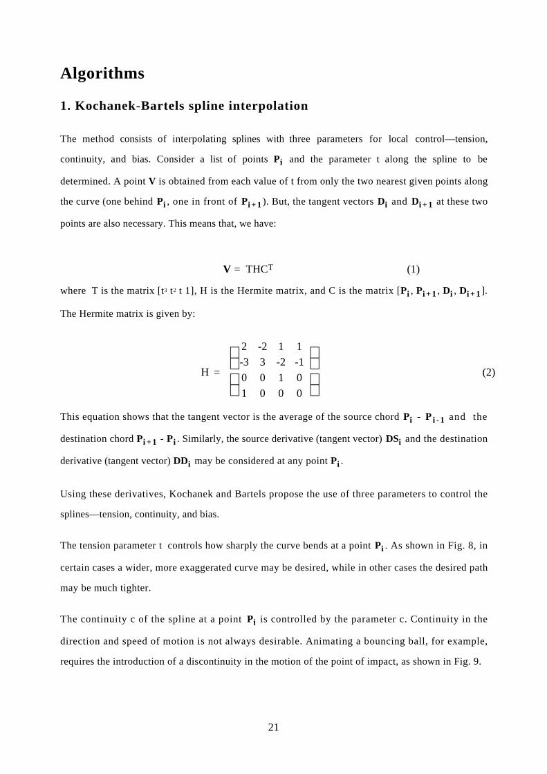
1. Kochanek-Bartels spline interpolation

The method consists of interpolating splines with three parameters for local control—tension,

continuity, and bias. Consider a list of points Pi and the parameter t along the spline to be

determined. A point V is obtained from each value of t from only the two nearest given points along

the curve (one behind Pi , one in front of Pi + 1 ). But, the tangent vectors Di and Di + 1 at these two

points are also necessary. This means that, we have:

V = THCT (1)

where T is the matrix [t3 t2 t 1], H is the Hermite matrix, and C is the matrix [Pi , Pi + 1 , Di , Di + 1 ].

The Hermite matrix is given by:

H =

2 -2 1 1

-3 3 -2 -1

0 0 1 0

1 0 0 0

(2)

This equation shows that the tangent vector is the average of the source chord Pi - P i - 1 and the

destination chord Pi + 1 - Pi . Similarly, the source derivative (tangent vector) DSi and the destination

derivative (tangent vector) DDi may be considered at any point Pi .

Using these derivatives, Kochanek and Bartels propose the use of three parameters to control the

splines—tension, continuity, and bias.

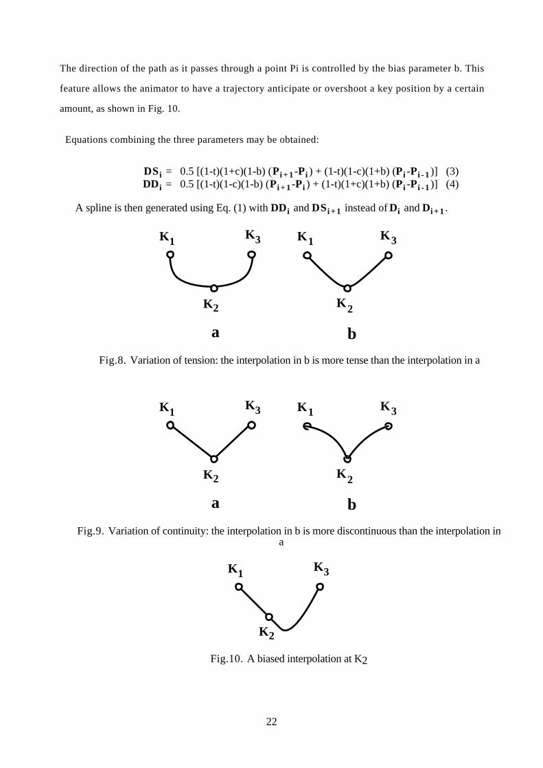
The tension parameter t controls how sharply the curve bends at a point Pi . As shown in Fig. 8, in

certain cases a wider, more exaggerated curve may be desired, while in other cases the desired path

may be much tighter.

The continuity c of the spline at a point Pi is controlled by the parameter c. Continuity in the

direction and speed of motion is not always desirable. Animating a bouncing ball, for example,

requires the introduction of a discontinuity in the motion of the point of impact, as shown in Fig. 9.

22

The direction of the path as it passes through a point Pi is controlled by the bias parameter b. This

feature allows the animator to have a trajectory anticipate or overshoot a key position by a certain

amount, as shown in Fig. 10.

Equations combining the three parameters may be obtained:

DS i = 0.5 [(1-t)(1+c)(1-b) (Pi + 1 -Pi ) + (1-t)(1-c)(1+b) (Pi -Pi - 1 )] (3)DDi = 0.5 [(1-t)(1-c)(1-b) (Pi + 1 -Pi ) + (1-t)(1+c)(1+b) (Pi -Pi - 1 )] (4)

A spline is then generated using Eq. (1) with DDi and DS i + 1 instead of Di and Di + 1 .

K3K1

K2

K1

K2

K3

a b

Fig.8. Variation of tension: the interpolation in b is more tense than the interpolation in a

K3K1

K2

K1

K2

K3

a b

Fig.9. Variation of continuity: the interpolation in b is more discontinuous than the interpolation ina

K3K1

K2

Fig.10. A biased interpolation at K2

23

2. Dynamic Simulation

Direct Dynamic

The most popular algorithm in dynamic simulation is Armstrong-Green algorithm, based on

Newton-Euler formulations. To get a simplified form in order to avoid the inversion of matrices

larger than three by three, two hypotheses have be made. The first assumes the linear relationship

between the linear acceleration of the link and the amount of angular acceleration it undergoes. The

second is the linear relationship between the linear acceleration and the reactive force on its parent

link. The algorithm can be divided to two opposite processes, inbound and outbound. The inbound

calculates some matrices and vectors from the geometric and physical structure of the system, and

propagates force and torque along each link from leaves to the root of the hierarchy. The outbound

calculates kinematics quantities, the linear and angular acceleration of each link, then to get the

linear and angular velocity by numerical integration for updating the whole structure. It is a

recursive algorithm along the whole time of dynamic simulation. The kinematic results of the former

time step are used as an initial values of the next step calculation.

Inverse Dynamics

The inverse dynamics problem is to find at each joint the force and torque that generate the desired

motion of the structure. Among many formulations, we select a kind of recursive formulation based

on Newton-Euler equations for their computational efficiency. The best advantage is that the

computation time is linearly proportional to the number of joints and independent of the limb

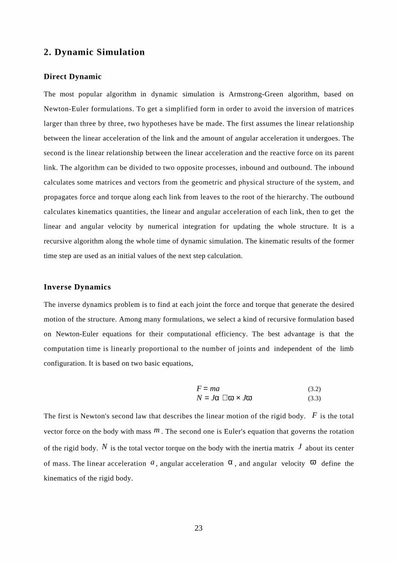
configuration. It is based on two basic equations,

F = ma (3.2)

N = Jα + ω × Jω (3.3)

The first is Newton's second law that describes the linear motion of the rigid body. F is the total

vector force on the body with mass m . The second one is Euler's equation that governs the rotation

of the rigid body. N is the total vector torque on the body with the inertia matrix J about its center

of mass. The linear acceleration a , angular acceleration α , and angular velocity ω define the

kinematics of the rigid body.

24

To construct the formulations for an articulated body model, we should write a series equations for

each link, using constrained forces and torque to guarantee their connection. The details of this

formulation for inverse dynamics is listed below. We can see it has two opposite process. The

forward recursion starts from the inertial coordinate frame to the end-effector coordinate frame to

forward propagate kinematics information. The backward recursion propagates the forces and

moments exerted on each link from the opposite direction.

Recursive Newton-Euler Algorithm

All vectors with subscript i are expressed in the body coordination frame of the ith link. The

following items except mi are vectors.

˙ q ij , ˙ ̇ q ij : the first and second derives of generalized variable for the jth DOF of the ith joint.

ω i : angular velocity of the ith link.

α i : angular acceleration of the ith link.

a i : linear acceleration of the ith link at the origin of its local coordination frame.

aci : linear acceleration of the ith link at the center of mass.

g : gravitational acceleration vector in the inertial coordination frame.

gi : gravitation of the ith link.

f i : force exerted on the ith link by the (i-1)st link.

ni : moment exerted on the ith link by the (i-1)st link.

τ i : joint generalized actuator torque at the ith joint.

pi : vector from the origin of ith link to the origin of (i+1)st link.

si : vector from the origin of ith link to its center of mass.

zij : rotation vector of the jth DOF of the ith joint.

mi : mass of link i.

Fi : total external force exerted on the ith link.

Ni : total external torque exerted on the ith link.

The following items are 3 by 3 matrix:

Ji : inertia matrix of the ith link.

Aij : pure rotational matrix from the jth link coordination frame to the ith.

Integer ndi : number of DOF at joint i.

The algorithm works as follows:

25

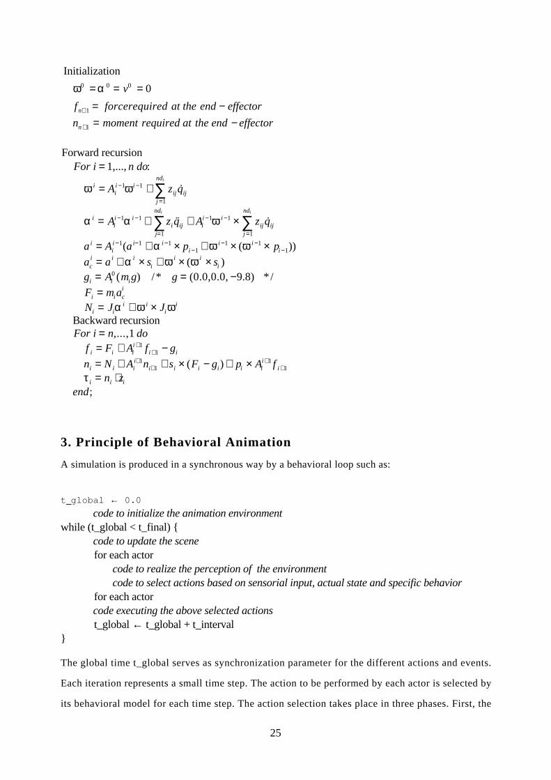
Initialization

ω0 = α 0 = v0 = 0

fn+ 1 = forcerequired at the end − effector

nn +1 = moment required at the end − effector

Forward recursionFor i = 1,..., n do:

ω i = Aii −1ω i −1 + zij ˙ q ij

j =1

ndi

∑

α i = Aii −1α i −1 + zi ˙ ̇ q ij

j=1

ndi

∑ + Aii −1ω i −1 × zij ˙ q ij

j =1

ndi

∑a i = Ai

i −1(a i−1 + α i −1 × pi −1 + ω i −1 × (ω i −1 × pi −1))

aci = a i + α i × si + ω i × (ω i × si )

gi = Ai0 (mig) /* g = (0.0,0.0, −9.8) * /

Fi = miaci

Ni = Jiαi + ω i × Jiω

i

Backward recursionFor i = n,...,1 do

f i = Fi + Aii +1 f i +1 − gi

ni = N i + Aii+1ni+1 + si × (Fi − gi) + pi × Ai

i +1 f i +1

τ i = ni ⋅ zi

end;

3. Principle of Behavioral Animation

A simulation is produced in a synchronous way by a behavioral loop such as:

t_global ← 0.0

code to initialize the animation environmentwhile (t_global < t_final) {

code to update the scenefor each actor

code to realize the perception of the environmentcode to select actions based on sensorial input, actual state and specific behavior

for each actorcode executing the above selected actionst_global ← t_global + t_interval

}

The global time t_global serves as synchronization parameter for the different actions and events.

Each iteration represents a small time step. The action to be performed by each actor is selected by

its behavioral model for each time step. The action selection takes place in three phases. First, the

26

actor perceives the objects and the other actors in the environment, which provides information on

their nature and position. This information is used by the behavioral model to decide the action to

take, which results in a motion procedure with its parameters: e.g. grasp an object or walk with a new

speed and a new direction. Finally, the actor performs the motion.

Research Issues and Summary

Computer Animation should not be just considered as a tool to enhance spatial perception by

moving the virtual camera or just rotating objects. More sophisticated animation techniques than

keyframe animation must be widely used. Computer animation tends to be more and more based

on physics and dynamic simulation methods. In the future, the application of computer animation

to the scientific world will also become very common in many scientific areas: fluid dynamics,

molecular dynamics, thermodynamics, plasma physics, astrophysics etc. Real-time complex

animation systems will be developed taking advantage of VR-devices and simulation methods. An

integration between simulation methods and VR-based animation will lead to systems allowing the

user to interact with complex time-dependent phenomena providing interactive visualization and

interactive animation. Moreover, real-time synthetic actors will be part of Virtual Worlds and people

will communicate with them through broadband multimedia networks. This development will be

only possible by developing new approaches to real-time motion.

Defining Terms

Behavioral animation: behavior of objects is driven by providing high-level directives indicating a

specific behavior without any other stimulus

L-systems: production-based approach to generate any concept of growth and life development in

the resulting animation.

Metaballs: shapes based on implicit surfaces; they are employed to simulate the gross behavior of

bone, muscle, and fat tissue.

27

Morphing or shape transformation: metamorphosis of an object into another object over time.

Image morphing manipulates two-dimensional images instead of three-dimensional objects and

generates a sequence of inbetween images from two images.

Parametric keyframe animation: the animator creates keyframes by specifying the appropriate set

of parameter values. Parameters are then interpolated and images are finally individually

constructed from the interpolated parameters

Performance animation consist of measurement and recording of direct actions of a real person or

animal for immediate or delayed analysis and playback

Procedural animation: corresponds to the creation of a motion by a procedure describing

specifically the motion. Procedural animation may be specified using a programming language or

interactive system

Rational Free Form Deformations: extension of the classical Free Form Deformations. Physically,

they correspond to weighted deformations applied to an imaginary parallelepiped of clear, flexible

plastic in which are embedded the object(s) to be deformed.

Spacetime Constraints: method for creating automatic character motion by specifying what the

character has to be, how the motion should be performed, what the character's physical structure is,

and what physical resources are available to the character to accomplish the motion.

Virtual sensors: used as a basis for implementing everyday human behaviour such as visually

directed locomotion, handling objects, and responding to sounds and utterances. Virtual humans

should be equipped with visual, tactile and auditory sensors.

ReferencesAono, M. 1990. A Wrinkle Propagation Model for Cloth, Proc. Computer Graphics International

'90, Springer, Tokyo, pp.96-115.

Armstrong, W.W., Green, M., and Lake, R. 1987. Near real-time Control of Human Figure Models,

28

IEEE Computer Graphics and Applications, Vol.7, No 6, pp.28-38

Badler, N.I., Phillips, C.B., and Webber, B.L. 1993. Simulating Humans: Computer Graphics

Animation and Control. Oxford University Press, New York, NY,.

Bandi S. and Thalmann, D. 1995. An Adaptive Spatial Subdivision of the Object Space for Fast

Collision of Animated Rigid Bodies, Proc. Eurographics ‘95, Maastricht, August 1995,

pp.259-270.

Baraff, D. 1989. Analytical Methods for Dynamic Simulation of Non-Penetrating Rigid Bodies,

Proc. SIGGRAPH '89, Computer Graphics, Vol. 23, No3, pp.223-232.

Boulic, R. Thalmann, D. and Magnenat-Thalmann N. 1990. A Global Human Walking Model with

Real Time Kinematic Personification. The Visual Computer, 6(6),.

Boulic, R., Capin, T., Huang, Z., Moccozet, L., Molet, T., Kalra, P., Lintermann, B., Magnenat-

Thalmann, N., Pandzic, I., Saar, K.,Schmitt, A., Shen, J. and Thalmann, D. 1995. The

HUMANOID Environment for Interactive Animation of Multiple Deformable Human

Characters, Proc. Eurographics ‘95, Maastricht, August 1995, pp.337-348.

Bruderlin, A. and Calvert T.W. 1989. Goal Directed, Dynamic Animation of Human Walking, Proc.

SIGGRAPH '89, Computer Graphics, Vol. 23, No3, 1989, pp.233-242

Carignan, M. Yang, Y. Magnenat Thalmann, N., and Thalmann, D. 1992. Dressing Animated

Synthetic Actors with Complex Deformable Clothes, Proc. SIGGRAPH '92, Computer

Graphics, Vol. 26, No.2, pp.99-104.

Chadwick, J.E., Haumann, D.R., and Parent, R.E. 1989. Layered construction for deformable

animated character, Computer Graphics, 23, (3), pp.243-252

Cohen, M.F. 1992. Interactive Spacetime Control for Animation Proc. Siggraph'92, pp.293-302.

Ekman, P. and Friesen, W. 1978. Facial Action Coding System, Consulting Psychologists Press, Palo

Alto.

Girard, M. and Maciejewski, AA. 1985. Computational Modeling for Computer Generation of

Legged Figures, Proc. SIGGRAPH '85, Computer Graphics, Vol. 19, No3, pp.263-270

Gourret, J.P. Magnenat-Thalmann, N. and Thalmann, D. 1989. Simulation of Object and Human

Skin Deformations in a Grasping Task, Proc. SIGGRAPH '89, Computer Graphics, Vol. 23, No

3, pp. 21-30

Hahn, J.K. 1988. Realistic Animation of Rigid Bodies, Proc. SIGGRAPH '88, Computer Graphics,

Vol. 22, No 4, pp.299-308.

Jianhua, S. and Thalmann, D. Interactive shape design using metaballs and splines, Proc. Implicit

29

Surfaces ‘95, Ggrenoble.

Kalra, P. Mangili, A. Magnenat-Thalmann, N. and Thalmann, D. 1992. Simulation of Facial Muscle

Actions Based on Rational Free Form Deformations, Proc. Eurographics '92, Cambridge, UK,.

Kochanek, D.H. and Bartels, R.H. 1984. Interpolating Splines with Local Tension, Continuity, and

Bias Control, Proc. SIGGRAPH '84, Computer Graphics, Vol. 18, pp.33-41

Kunii, T.L. and Gotoda, H. 1990. Modeling and Animation of Garment Wrinkle Formation

Processes, Proc. Computer Animation '90, Springer, Tokyo, pp.131-147.

Lafleur, B. Magnenat Thalmann, N., and Thalmann, D. 1991. Cloth Animation with Self-Collision

Detection. In Proc. IFIP Conference on Modeling in Computer Graphics, Springer, Tokyo,

pp.179-187.

Lee, S. and Shin S.Y. 1995. Warp Generation and Transition Control in Image Morphing in:

Magnenat Thalmann, N. and Thalmann D. (eds) Interactive Computer Animation, Prentice

Hall,.

Magnenat Thalmann, N. and Thalmann, D. 1990, Computer Animation: Theory and Practice,

Springer Verlag, Tokyo, 2nd edition.

Magnenat Thalmann, N. and Thalmann, D. 1991. Complex Models for Animating Synthetic Actors,

IEEE Computer Graphics and Applications, Vol.11, September.

Magnenat Thalmann, N. and Thalmann, D. 1985. 3D Computer Animation: More an Evolution

Problem than a Motion Problem, IEEE Computer Graphics and Applications, Vol.5, No 10,

pp. 47-57.

Magnenat-Thalmann, Laperrière, R., and Thalmann, D. 1988. Joint-Dependent Local Deformations

for Hand Animation and Object Grasping, Proc. Graphics Interface'88, Edmonton, pp.26-33

Magnenat-Thalmann, N. Primeau, E. and Thalmann, D. 1988. Abstract Muscle Action Procedures

for Human Face Animation, The Visual Computer, Vol. 3, No. 5, pp. 290-297.

Maiocchi R. 1995. 3D Character Animation Using Motion Capture, in: Magnenat Thalmann, N. and

Thalmann D. (eds) Interactive Computer Animation, Prentice Hall,.

Mas, R. and Thalmann D. 1994. A Hand Control and Automatic Grasping System for Synthetic

Actors, Proceedings of Eurographic'94, pp.167-178.

Mase, K. and Pentland, A. 1990. Automatic Lipreading by Computer Trans. Inst. Elec. Info. and

Comm. Eng., Vol. J73-D-II, No. 6, 796-803

McKenna, M. and Zeltzer D. 1990. Dynamic Simulation of Autonomous Legged Locomotion,

Proc. SIGGRAPH '90, Computer Graphics, Vol. 24, No 4, pp.29-38.

30

Noser, H. and Thalmann, D. 1995. Synthetic Vision and Audition for Digital Actors, Proc.

Eurographics ‘95, Maastricht, August 1995, pp.325-336.

Noser, H. Renault, O. Thalmann, D. and Magnenat Thalmann, N. 1995. ”Navigation for Digital

Actors based on Synthetic Vision, Memory and Learning”, Computers and Graphics,

Pergamon Press, Vol.19, No1, pp.7-19.

Noser, H. Turner, R., and Thalmann, D. 1992. Interaction between L-systems and Vector Force-

Field, Proc. Computer Graphics International '92, Tokyo, pp.747-761.

Pandzic, I.S., Kalra, P., and Magnenat-Thalmann N. “Real Time Facial Interaction”, Displays, Vol.

15, No. 3, 1994, pp. 157-163.

Parke, F.I. 1982. Parameterized Models for Facial Animation, IEEE Computer Graphics and

Applications, Vol.2, No 9, pp.61-68

Platt, S. and Badler, N. 1981. Animating Facial Expressions, Proc. SIGGRAPH '81, Computer

Graphics, Vol.15, No3, pp.245-252.

Renault, O. Magnenat-Thalmann, N. and Thalmann, D. 1990. A Vision-Based Approach to

Behavioural Animation, Visualization and Computer Animation Journal, John Wiley, Vol.1,

No1, 1990, pp.18-21.

Reynolds C. 1987. Flocks, Herds, and Schools: A Distributed Behavioral Model, Proc.SIGGRAPH

'87, Computer Graphics, Vol.21, No4, pp.25-34

Reynolds, C.W. 1993. ”An Evolved, Vision-Based Behavioral Model of Coordinated Group

Motion”, in: Meyer J.A. et al. (eds) From Animals to Animats, Proc. 2nd International Conf.

on Simulation of Adaptive Behavior, MIT Press, pp.384-392.

Ridsdale G. 1990. Connectionist Modelling of Skill Dynamics, Journal of Visualization and

Computer Animation, Vol.1, No2, pp.66-72.

Rijpkema, H. and Girard, M. 1991. Computer Animation of Knowledge-based Grasping, Proc.

SIGGRAPH ‘91, Computer Graphics, vol. 25, N. 4, pp:339-348.

Saji, H. Hioki, H. Shinagawa, Y. Yoshida, K. Kunii T.L. 1992. Extraction of 3D Shapes from the

Moving Human Face using Lighting Switch Photometry in Magnenat Thalmann, N. and

Thalmann D. (Eds) Creating and Animating the Virtual World, Springer-Verlag Tokyo, 69-86

Terzopoulos, D. Platt, J.C. Barr, A.H., and Fleischer, K. 1987. Elastically Deformable Models,

Proc.SIGGRAPH'87, Computer Graphics, Vol. 21 No 4, pp.205-214

Thalmann, D. 1990. Robotics Methods for Task-level and Behavioral Animation, in: Thalmann D

(ed) Scientific Visualization and Graphics Simulation, John Wiley, Chichester, UK, pp.129-

31

147.

Thalmann, D. 1993. Using Virtual Reality Techniques in the Animation Process, In: Earnshaw, R.

Gigante, Jones M.H. (eds) Virtual Reality Systems, Academic Press.

Thalmann, N.M. and Thalmann, D. 1987. The Direction of Synthetic Actors in the Film Rendez-

vous a Montreal, IEEE CG&A, Vol.7, No12, pp.9-19.

Tu, X. and Terzopoulos D. 1994. ”Artificial Fishes: Physics, Locomotion, Perception, Behavior”,

Proc. SIGGRAPH '94, Computer Graphics, pp.42-48.

Volino P., Courchesnes, M., and Magnenat Thalmann, N. 1995 Versatile and Efficient Techniques

for Simulating Cloth and Other Deformable Objects, Proc. SIGGRAPH ‘95.

Volino, P., and Magnenat Thalmann, N. 1994. Efficient Self-Collision Detection on Smoothly

Discretised Surface Animations using Geometrical Shape Regularity, Proc. Eurographics ‘94,

Computer Graphics Forum, 13(3), pp.155-166.

Waters K. 1987. A Muscle Model for Animating Three-Dimensional Facial Expression, Proc.

SIGGRAPH '87, Computer Graphics, Vol.21, No4, pp.17-24.

Waters, K. and Terzopoulos, D. 1991. “Modeling and Animating Faces using Scanned Data”, The

Journal of Visualization and Computer Animation, Vol. 2, No. 4, pp. 123-128.

Weil, J. 1986. The Synthesis of Cloth Objects. In Proc. SIGGRAPH'86, Computer Graphics, Vol.20,

No.4, pp.49-54.

Wilhelms J. 1990. A “Notion” for Interactive Behavioral Animation Control, IEEE Computer

Graphics and Applications , Vol. 10, No 3 , pp.14-22

Williams, L. 1990. Performance Driven Facial Animation, Proc SIGGRAPH '90, pp. 235-242.

Witkin, A. and Kass, M. 1988. Spacetime Constraints, Proc. SIGGRAPH '88, Computer Graphics,

Vol.22, No4 , pp.159-168.

Wolberg G. 1990 “Digital Image Warping“, IEEE Computer Society Press,.

Zeltzer D. 1982. Motor Control Techniques for Figure Animation, IEEE Computer Graphics and

Applications , Vol. 2, No9 , pp.53-59.

Zeltzer, D. 1985. Towards an Integrated View of 3D Computer Animation, The Visual Computer,

Vol. 1, No4, pp.249-259

Further informationSeveral textbooks on Computer Animation have been published:

32

1. N. Magnenat Thalmann, D.Thalmann (eds) Computer Animation: Theory and Practice,

Springer Verlag, Tokyo (2nd edition), 1990

2. J. Vince, 3-D Computer Animation, Addison-Wesley, 1992

3. S. Mealing, The Art and Science of Computer Animation, Intellect, Oxford, UK, 1992

4. N. Magnenat Thalmann, D.Thalmann (eds) Interactive Computer Animation, Prentice Hall,

1996 (to appear)

There is one journal dedicated to Computer Animation, The Journal of Visualization and Computer

animation published by John Wiley and Sons, Chichester, UK since 1990.

Although Computer Animation is always represented in major Computer Graphics conferences like

SIGGRAPH, Computer Graphics International (CGI), Pacific Graphics, and Eurographics, there are

only two annual conferences dedicated to Computer Animation:

1. Computer Animation, organized each year in Geneva by the Computer Graphics Society.

Proceedins are published by IEEE Computer Society Press.

2. Eurographics workshop on Animation and Simulation organized each year by

Eurographics.