
Computed tear film and osmolarity dynamics on an eye ... · At the ocular surface, there is a...
35
doi:10.1093/imammb/dqv013 Computed tear film and osmolarity dynamics on an eye-shaped domain Longfei Li † , Richard J. Braun ∗ and Tobin A. Driscoll Department of Mathematical Sciences, University of Delaware, Newark, DE 19711, USA ∗ Corresponding author. Email: [email protected] William D. Henshaw Department of Mathematical Sciences, Rensselaer Polytechnic Institute, Troy, NY 12180, USA Jeffrey W. Banks † Lawrence Livermore National Laboratory, Box 808, L-422, Livermore, CA 94551-0808, USA and P. Ewen King-Smith College of Optometry, The Ohio State University, Columbus, OH 43218, USA [Received on May 26, 2014; revised on December 23, 2014; accepted on March 12, 2015] The concentration of ions, or osmolarity, in the tear film is a key variable in understanding dry eye symp- toms and disease. In this manuscript, we derive a mathematical model that couples osmolarity (treated as a single solute) and fluid dynamics within the tear film on a 2D eye-shaped domain. The model includes the physical effects of evaporation, surface tension, viscosity, ocular surface wettability, osmolarity, osmo- sis and tear fluid supply and drainage. The governing system of coupled non-linear partial differential equations is solved using the Overture computational framework, together with a hybrid time-stepping scheme, using a variable step backward differentiation formula and a Runge–Kutta–Chebyshev method that were added to the framework. The results of our numerical simulations provide new insight into the osmolarity distribution over the ocular surface during the interblink. Keywords: lubrication theory; osmolarity dynamics; tear film; thin film; composite overlapping grid. 1. Introduction The purpose of the model we develop here is to compute the dynamics of fluid motion and osmolarity of the tear film on an eye-shaped domain. Osmolarity is the concentration of ions in solution. Given an 1M concentration of NaCl solution, each molecule of salt dissociates into two ions, and the osmolarity is then 2 M. (Here M denotes molar concentration, which is moles per litre of solvent.) For a brief introduction to the mathematical models for the osmolarity and tear film dynamics, see the review by Braun (2012) or the paper by Zubkov et al. (2012). The osmolarity is an important variable to include in tear film modelling because it is thought to be critical in the onset and subsequent development of dry eye syndrome (DES). A properly functioning tear film maintains a critical balance between tear secretion and loss within each blink cycle. Malfunc- tion or deficiency of the tear film causes a collection of problems that are believed to comprise DES (Lemp, 2007). DES symptoms include, but are not limited to, blurred vision, burning, foreign body † Present address: Department of Mathematical Sciences, Rensselaer Polytechnic Institute, Troy, NY 12180, USA. c The authors 2015. Published by Oxford University Press on behalf of the Institute of Mathematics and its Applications. All rights reserved. Mathematical Medicine and Biology (2016) 33, 123–157 Advance Access publication on April 15, 2015 Downloaded from https://academic.oup.com/imammb/article-abstract/33/2/123/2875345 by University of Delaware Library user on 07 June 2019
Transcript of Computed tear film and osmolarity dynamics on an eye ... · At the ocular surface, there is a...
doi:10.1093/imammb/dqv013
Computed tear film and osmolarity dynamics on an eye-shaped domain
Longfei Li†, Richard J. Braun∗ and Tobin A. Driscoll
Department of Mathematical Sciences, University of Delaware, Newark, DE 19711, USA∗Corresponding author. Email: [email protected]
William D. Henshaw
Department of Mathematical Sciences, Rensselaer Polytechnic Institute, Troy, NY 12180, USA
Jeffrey W. Banks†
Lawrence Livermore National Laboratory, Box 808, L-422, Livermore, CA 94551-0808, USA
and
P. Ewen King-Smith
College of Optometry, The Ohio State University, Columbus, OH 43218, USA
[Received on May 26, 2014; revised on December 23, 2014; accepted on March 12, 2015]
The concentration of ions, or osmolarity, in the tear film is a key variable in understanding dry eye symp-toms and disease. In this manuscript, we derive a mathematical model that couples osmolarity (treated as asingle solute) and fluid dynamics within the tear film on a 2D eye-shaped domain. The model includes thephysical effects of evaporation, surface tension, viscosity, ocular surface wettability, osmolarity, osmo-sis and tear fluid supply and drainage. The governing system of coupled non-linear partial differentialequations is solved using the Overture computational framework, together with a hybrid time-steppingscheme, using a variable step backward differentiation formula and a Runge–Kutta–Chebyshev methodthat were added to the framework. The results of our numerical simulations provide new insight into theosmolarity distribution over the ocular surface during the interblink.
Keywords: lubrication theory; osmolarity dynamics; tear film; thin film; composite overlapping grid.
1. Introduction
The purpose of the model we develop here is to compute the dynamics of fluid motion and osmolarityof the tear film on an eye-shaped domain. Osmolarity is the concentration of ions in solution. Given an1M concentration of NaCl solution, each molecule of salt dissociates into two ions, and the osmolarityis then 2 M. (Here M denotes molar concentration, which is moles per litre of solvent.) For a briefintroduction to the mathematical models for the osmolarity and tear film dynamics, see the review byBraun (2012) or the paper by Zubkov et al. (2012).
The osmolarity is an important variable to include in tear film modelling because it is thought to becritical in the onset and subsequent development of dry eye syndrome (DES). A properly functioningtear film maintains a critical balance between tear secretion and loss within each blink cycle. Malfunc-tion or deficiency of the tear film causes a collection of problems that are believed to comprise DES(Lemp, 2007). DES symptoms include, but are not limited to, blurred vision, burning, foreign body
†Present address: Department of Mathematical Sciences, Rensselaer Polytechnic Institute, Troy, NY 12180, USA.
c© The authors 2015. Published by Oxford University Press on behalf of the Institute of Mathematics and its Applications. All rights reserved.
Mathematical Medicine and Biology (2016) 33, 123–157
Advance Access publication on April 15, 2015
Dow
nloaded from https://academ
ic.oup.com/im
amm
b/article-abstract/33/2/123/2875345 by University of D
elaware Library user on 07 June 2019
L. LI ET AL.
sensation, tearing and inflammation of the ocular surface. Studies up to 2007 estimate that there are4.91 million Americans suffering from DES (Anonymous, 2007). The ocular surface community isinterested in understanding the function of the tear film (Johnson & Murphy, 2004) as well as the inter-action of tear film dynamics and the connection between tear film volume, evaporation and break-upwith DES (Anonymous, 2007).
We summarize a discussion of the role of osmolarity on the ocular surface from Baudouin et al.(2013) here. According to Tietz (1995), in healthy blood the osmolarity is in the range 285–295 Osm/m3
(also expressed in mOsm/L or mOsM). In the healthy tear film, there is homoeostasis with the blood inthe range 296–302 Osm/m3 (Tomlinson et al., 2006; Versura et al., 2010; Lemp et al., 2011). In DES,the lacrimal system is unable to maintain this homoeostasis and osmolarity values in the meniscus riseto 316–360 Osm/m3 (Gilbard et al., 1978; Tomlinson et al., 2006; Sullivan et al., 2010), and may riseto even higher values over the cornea. Using in vivo experiment and sensory feedback, Liu et al. (2009)estimated peak values of 800–900 Osm/m3. Similar or higher values were computed from mathematicalmodels of tear film break-up in King-Smith et al. (2010b) and Peng et al. (2014). We use a mathematicalmodel to compute osmolarity over the entire exposed ocular surface subject to the assumptions statedin the Formulation section.
The method of tear sample collection and measurement is important. To our knowledge, osmolaritymeasurements in humans have been from samples in the inferior meniscus or the lower fornix. Thelower fornix has a lower osmolarity than the meniscus (Mishima et al., 1971), and samples from themeniscus are most commonly used today. Gilbard et al. (1978) summarized the use of prior measure-ment techniques that used pipettes or capillary tubes to collect tear samples. Older methods may haveused pipettes that took too large a sample compared with the tear film total volume, and could inducereflex tearing. In the exquisitely sensitive eye, this is a significant concern that could dilute or otherwisechange the chemistry of the tear sample. Some capillary techniques are difficult to use, and the methodof Gilbard et al. (1978) appeared to be easier to use; we note that the paper does not indicate wherein the inferior meniscus the measurement was taken. Subsequent to sample collection, older techniquesrelied on freezing point depression to determine the osmolarity of the sample to about 1% error. Morerecently, a calibrated resistance measurement using the TearLab device allows rapid determination ofosmolarity with an error for in vitro samples of about 1–2% error (Lemp et al., 2011; TearLab, 2013).In the approach, a sensor touches the meniscus at the temporal canthus, and the result is returned in lessthan a minute after the sample is taken. The latter approach is much more convenient for clinical use.
The level of effectiveness of osmolarity measurement to diagnose dry eye and to measure pro-gression of the disease is still a matter of debate; for recent viewpoints, see for example Lemp et al.(2011), Amparo et al. (2013, 2014), Pepose et al. (2014) and Sullivan (2014). We found the summaryby Baudouin et al. (2013) in their Sections 3 and 4 to be informative. We do not aim to settle thedebate here, but to supply context for the measurements in the form of a quantitative prediction of theosmolarity over the entire exposed ocular surface to aid interpretation.
We now turn to previous work on the properties and dynamics of the tear film, relying heavilyon the introduction from Li et al. (2014). Commonly, the tear film is described as a thin liquid filmwith multiple layers. At the anterior interface with air is an oily lipid layer that decreases the surfacetension and retards evaporation, both of which help to retain a smooth well-functioning tear film (Norn,1979). The aqueous layer is posterior to the lipid layer and consists mostly of water (Holly, 1973).At the ocular surface, there is a region with transmembrane mucins protruding from the cells in thecorneal or conjunctival epithelia. This forest of glycosylated mucins, called the glycocalyx, has beenreferred to as the mucus layer in the past. It is generally agreed that the presence of the hydrophilicglycocalyx on the ocular surface prevents the tear film from dewetting (Bron et al., 2004; Gipson, 2004;
124
Dow
nloaded from https://academ
ic.oup.com/im
amm
b/article-abstract/33/2/123/2875345 by University of D
elaware Library user on 07 June 2019

COMPUTED TEAR FILM AND OSMOLARITY DYNAMICS ON AN EYE-SHAPED DOMAIN
Govindarajan & Gipson, 2010). The overall thickness of the tear film is a few microns (King-Smithet al., 2004), while the average thickness of the lipid layer is on the order of 50–100 nm (Norn, 1979;King-Smith et al., 2011) and the thickness of the glycocalyx is a few tenths of a micron (Govindarajan& Gipson, 2010). This structure is rapidly reformed, on the order of one second, after each blink in aproperly functioning tear film.
The aqueous part of tear fluid is supplied from the lacrimal gland near the temporal canthus and theexcess is drained through the puncta near the nasal canthus. Mishima et al. (1966) estimated the totaltear volume and the rate of influx from the lacrimal gland, as well as the time for the entire volumeof tear fluid to be replaced (tear turnover rate); Zhu & Chauhan (2005) reviewed experiments on teardrainage and developed a mathematical model for drainage rates of the aqueous component through thepuncta. Doane (1981) proposed the mechanism of tear drainage in vivo whereby tear fluid is drainedinto the canaliculi through the puncta during the opening interblink phase. The drainage stops whenthe pressure equalizes in the canaliculi. Water lost from the tear film due to evaporation into air is animportant process as well (Mishima & Maurice, 1961; Tomlinson et al., 2009; Kimball et al., 2010).This is the primary mechanism by which the osmolarity is increased in the tear film.
The supply and drainage of tear fluid affects the distribution and flow of the tear film. A number ofmethods have been used to visualize and/or measure tear film thickness and flow, including interferom-etry (Doane, 1989; King-Smith et al., 2004; King-Smith et al., 2009), optical coherence tomography(Wang et al., 2003), fluorescence imaging (Harrison et al., 2008; King-Smith et al., 2013) and manyothers. We mention only a small number here that are relevant for our discussion of tear fluid flowover the exposed ocular surface. Maurice (1973) inserted lampblack into the tear film and watched theparticle trajectories with a slit lamp. He observed that the particle paths in the upper meniscus nearthe temporal canthus diverge, with some particles proceeding towards the nasal canthus via the uppermeniscus and others going around the outer canthus before proceeding towards the nasal canthus via thelower meniscus. (To our knowledge, no images from this experiment exist.) We use the term ‘hydraulicconnectivity’ as shorthand for this splitting of flow connecting the menisci. A similar pattern of the tearfilm was observed by Harrison et al. (2008) using fluorescein to visualize the tear film thickness. Inthis experiment, concentrated sodium fluorescein is instilled in the eye. Shining blue light on the eyecauses the fluorescein to glow green; the fluorescence allows one to visualize the tear film (Lakowicz,2006). The concentration is such that if evaporation occurs, the concentration of fluorescein increasesand the intensity of the fluorescence decreases; if fresh tear fluid enters the tear film, the concentrationdecreases and fluorescent intensity increases (Webber & Jones, 1986; Nichols et al., 2012; Braun et al.,2014). Harrison et al. (2008) visualized the entry of fresh tear fluid into the meniscus near the outercanthus, where the tear film was observed to brighten. Subsequently, this bright region split and fluidmoved towards the nasal canthus along both the upper and lower lids via the menisci. The fluorescencecould thus visualize hydraulic connectivity in the flow of tears. Similar experiments in King-Smith et al.(2013) and Li et al. (2014) visualized flow by using fluorescein instilled by drops in the tear film, andthe mathematical model developed by Li et al. (2014) exhibited hydraulic connectivity in a very similarway to the experimental results shown in that paper.
The tear film is also redistributed near the eyelid margins by surface tension. The curvature generatedby the meniscus creates a low pressure which draws in fluid from surrounding areas, creating locallythin regions near the meniscus. When fluorescein is used to visualize tear film thickness, this locally thinregion near the lids is dark, and had been called the ‘black line’. The black line is typically thought to bea barrier between the meniscus at the lid margins and the rest of the tear film (McDonald & Brubaker,1971; Miller et al., 2002). Finally, though the healthy ocular surface is wettable, the tear film may stillrupture; the term break-up is used in the ocular science community for this phenomenon. The surface
125
Dow
nloaded from https://academ
ic.oup.com/im
amm
b/article-abstract/33/2/123/2875345 by University of D
elaware Library user on 07 June 2019

L. LI ET AL.
tension of the tear/air interface, the wettability of the ocular surface and the osmolarity are among theeffects that we include in this study.
A variety of mathematical models have incorporated various important effects of tear film dynamicsas recently reviewed by Braun (2012). The most common assumptions for these models are a Newtoniantear fluid and a flat cornea (Berger & Corrsin, 1974; Braun et al., 2012). Tear film models are oftenformulated on a 1D domain oriented vertically through the centre of the cornea with stationary endscorresponding to the eyelid margins. We refer to models on this kind of domain as 1D models. Surfacetension, viscosity, gravity and evaporation are often incorporated into 1D models (Wong et al., 1996;Sharma et al., 1998; Miller et al., 2002; Braun & Fitt, 2003). Winter et al. (2010) improved previousevaporation models by including a conjoining pressure from van der Waals forces that approximatedthe wettable corneal surface. Incorporating heat transfer from the underlying eye, Li & Braun (2012)resolved a discrepancy of the tear film surface temperature between predictions of existing evaporationmodels and in vivo measurements.
Recently, studies of 1D models that bring together the interblink period and a moving end that rep-resents the upper lid have appeared. Jones et al. (2005, 2006) developed models for tear film formationand relaxation that were unified in this way; one end of the domain moved to model the upper lid motionduring the opening phase of the blink, and then remained stationary for the subsequent relaxation duringthe interblink. The tear film was treated as a shear-thinning fluid without elasticity in an otherwise simi-lar model by Jossic et al. (2009) to try to tailor the viscosity of eye drops to obtain the most uniform tearfilm. Braun & King-Smith (2007) modelled eyelid motion for blink cycles by moving one end of thedomain sinusoidally and they computed solutions for multiple complete blink cycles. Heryudono et al.(2007) followed their study with a more realistic lid motion and specified a flux boundary condition.Good agreement on tear film thickness between experiments and simulations was found by Heryudonoet al. (2007). Deng et al. (2013, 2014) extended the model of Li & Braun (2012) to include upper lidmotion (blink) and heat transfer from the underlying eye to explain observed ocular surface temperaturemeasurements and to give new transient temperature results inside the eye. Bruna & Breward (2014)studied a model that added a dynamic lipid layer to an underlying aqueous layer with an insoluble sur-factant at the lipid/aqueous interface (representing polar lipids). They computed dynamic results for themodel and found various useful limits for it.
Braun (2012) gave a model for a spatially uniform film with no space dependence that was verysimilar to the one first suggested by King-Smith et al. (2007). The original model was a single ordinarydifferential equation for the tear film thickness that included evaporation from the tear/air interface ata constant rate and osmotic flow from the tear/cornea interface that was proportional to the osmolarityincrease above the isotonic value. The latter assumption simplifies the tear/cornea interface to a semi-permeable boundary that allows water but not solutes to pass. They found that the model predictedequilibration of the tear film thickness at values greater than the height of the glycocalyx for sufficientlylarge permeability of the tear/cornea interface. They also found that the osmolarity could become quitelarge as the tear film thinned for small permeability values, as much as 10 times the isotonic value undersome conditions. The model given in Braun (2012) included van der Waals forces that stopped thinningat the purported height of the glycocalyx which allowed the model to be used at zero permeability at thetear/cornea interface. Similar conclusions about the osmolarity during thinning were found there.
These models were extended to include a specified evaporation profile that varied in space by King-Smith et al. (2010b). The evaporation profile was Gaussian with a peak value that could be specifiedlarger than the surrounding constant rate. The local thinning caused by locally increased evaporationled to increased osmolarity in the break-up region, which could be several times larger than the isotonicvalue. A modified evaporation distribution was created by Peng et al. (2014) that had two parts. One part
126
Dow
nloaded from https://academ
ic.oup.com/im
amm
b/article-abstract/33/2/123/2875345 by University of D
elaware Library user on 07 June 2019

COMPUTED TEAR FILM AND OSMOLARITY DYNAMICS ON AN EYE-SHAPED DOMAIN
used an immobile lipid layer with specified thickness and fixed resistance to diffusion through it bywater. The other part was a resistance to transport in the air outside the tear film; this second resistanceincluded convective and diffusive transport in the air. They also found that the osmolarity was elevatedin this model for break-up.
Zubkov et al. (2012) developed a model describing the spatial distribution of tear film osmolaritythat incorporates both fluid and solute (osmolarity) dynamics, evaporation, blinking and vertical sac-cadic eyelid motion. They found that both osmolarity was increased in the black line region and thatmeasurements of the solute concentrations within the lower meniscus need not reflect those elsewhere inthe tear film. This model gave results over a line oriented vertically through the centre of the cornea, andthus gave information about the osmolarity over more of the ocular surface than the models mentionedabove.
In this paper, we study dynamics of the fluid motion and osmolarity on an eye-shaped domain. Toour knowledge, Maki et al. (2010a,b) were the first to extend models of fluid dynamics in the tear filmto a geometry that approximated the exposed ocular surface. They formulated a relaxation model on astationary 2D eye-shaped domain that was approximated from a digital photo of an eye. They specifiedtear film thickness and pressure boundary conditions (Maki et al., 2010a) or flux boundary conditions(Maki et al., 2010b). Their simulations recovered features seen in 1D models such as formation of theblack line, and captured some experimental observations of the tear film dynamics around the lid mar-gins. Maki et al. (2010b) simplified the in vivo mechanisms and imposed a flux boundary conditionhaving only spatial dependence (specifying the location of the lacrimal gland and the puncta holes) intheir tear film relaxation model. Under some conditions, they were able to recover hydraulic connectiv-ity as seen experimentally and described above. Li et al. (2014) improved the model, added evaporationand a wettable ocular surface, as well as a time-dependent boundary condition that approximated the in-and out-flow of the aqueous layer of the tear film.
In this paper, we formulate a tear film dynamics model on a 2D eye-shaped domain that, adding tothe previous models, incorporates osmolarity transport and osmosis from the tear/eye interface. To ourknowledge, this is the first such model that includes the osmolarity in a 2D tear film model and thatprovides a global osmolarity distribution over the entire exposed eye. The permeability of the ocularsurface is treated as either constant over the whole surface, or as a space-dependent function with lowerpermeability over the cornea and higher permeability over the conjunctiva. In the model, the tear filmloses water via evaporation to the air, gains water from the ocular surface, and, via the flux boundarycondition, has water supplied from the lacrimal gland and removed from the puncta. The model addssignificant new results about the distribution of osmolarity over the exposed ocular surface. We believethat these results will impact the understanding of osmolarity dynamics in the tear film as well as themeasurement of this important quantity.
We begin by formulating the model in Section 2. A brief description of the numerical methods usedfor the simulation is discussed in Section 3, followed by detailed results of simulations and comparisonwith experiments in Section 4. Conclusions and further directions are pointed out in Section 5.
2. Formulation
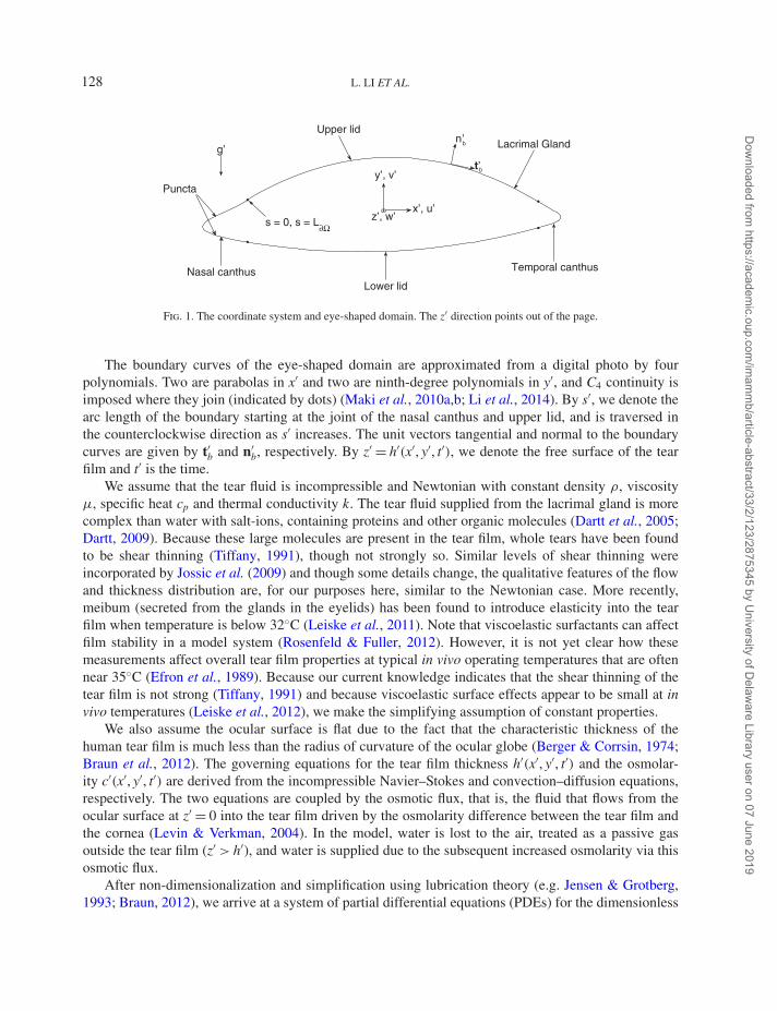
In this section, we present a mathematical model that incorporates osmolarity and fluid dynamics intoa tear film model on a 2D eye-shaped domain as shown in Fig. 1. In Fig. 1, (u′, v′, w′) are the velocitycomponents in the coordinate directions (x′, y′, z′); z′ is directed out of the page and primed variablesare dimensional. By g′, we denote gravity which is specified in the negative y′ direction.
127
Dow
nloaded from https://academ
ic.oup.com/im
amm
b/article-abstract/33/2/123/2875345 by University of D
elaware Library user on 07 June 2019
L. LI ET AL.
y’, v’
x’, u’z’, w’
t’
n’b
b
g’
Puncta
s = 0, s = L∂Ω
Lacrimal GlandUpper lid
Lower lid
Temporal canthusNasal canthus
Fig. 1. The coordinate system and eye-shaped domain. The z′ direction points out of the page.
The boundary curves of the eye-shaped domain are approximated from a digital photo by fourpolynomials. Two are parabolas in x′ and two are ninth-degree polynomials in y′, and C4 continuity isimposed where they join (indicated by dots) (Maki et al., 2010a,b; Li et al., 2014). By s′, we denote thearc length of the boundary starting at the joint of the nasal canthus and upper lid, and is traversed inthe counterclockwise direction as s′ increases. The unit vectors tangential and normal to the boundarycurves are given by t′b and n′
b, respectively. By z′ = h′(x′, y′, t′), we denote the free surface of the tearfilm and t′ is the time.
We assume that the tear fluid is incompressible and Newtonian with constant density ρ, viscosityμ, specific heat cp and thermal conductivity k. The tear fluid supplied from the lacrimal gland is morecomplex than water with salt-ions, containing proteins and other organic molecules (Dartt et al., 2005;Dartt, 2009). Because these large molecules are present in the tear film, whole tears have been foundto be shear thinning (Tiffany, 1991), though not strongly so. Similar levels of shear thinning wereincorporated by Jossic et al. (2009) and though some details change, the qualitative features of the flowand thickness distribution are, for our purposes here, similar to the Newtonian case. More recently,meibum (secreted from the glands in the eyelids) has been found to introduce elasticity into the tearfilm when temperature is below 32◦C (Leiske et al., 2011). Note that viscoelastic surfactants can affectfilm stability in a model system (Rosenfeld & Fuller, 2012). However, it is not yet clear how thesemeasurements affect overall tear film properties at typical in vivo operating temperatures that are oftennear 35◦C (Efron et al., 1989). Because our current knowledge indicates that the shear thinning of thetear film is not strong (Tiffany, 1991) and because viscoelastic surface effects appear to be small at invivo temperatures (Leiske et al., 2012), we make the simplifying assumption of constant properties.
We also assume the ocular surface is flat due to the fact that the characteristic thickness of thehuman tear film is much less than the radius of curvature of the ocular globe (Berger & Corrsin, 1974;Braun et al., 2012). The governing equations for the tear film thickness h′(x′, y′, t′) and the osmolar-ity c′(x′, y′, t′) are derived from the incompressible Navier–Stokes and convection–diffusion equations,respectively. The two equations are coupled by the osmotic flux, that is, the fluid that flows from theocular surface at z′ = 0 into the tear film driven by the osmolarity difference between the tear film andthe cornea (Levin & Verkman, 2004). In the model, water is lost to the air, treated as a passive gasoutside the tear film (z′ > h′), and water is supplied due to the subsequent increased osmolarity via thisosmotic flux.
After non-dimensionalization and simplification using lubrication theory (e.g. Jensen & Grotberg,1993; Braun, 2012), we arrive at a system of partial differential equations (PDEs) for the dimensionless
128
Dow
nloaded from https://academ
ic.oup.com/im
amm
b/article-abstract/33/2/123/2875345 by University of D
elaware Library user on 07 June 2019

COMPUTED TEAR FILM AND OSMOLARITY DYNAMICS ON AN EYE-SHAPED DOMAIN
variables h(x, y, t) and c(x, y, t):
∂th + EJ + ∇ · Q − Pc(c − 1) = 0, (2.1)
h∂tc + ∇c · Q = EcJ + 1
Pec∇ · (h∇c) − Pc(c − 1)c. (2.2)
The evaporative mass flux J is given by
J = 1 − δ(SΔh + Ah−3)
K̄ + h,
and the fluid flux Q across any cross-section of the film is given by
Q = h3
12∇(SΔh + Ah−3 − Gy).
The conjoining pressure in modelling evaporation plays an important role in the tear film model. Itis meant to mimic the effect of the glycocalyx, whose transmembrane are strongly wet by water andwe assume that they arrest the thinning of the tear film. A secondary benefit is that the model allowssolutions to be computed past the initial tear film break-up because the tear film thickness never reacheszero in this model. These aspects of evaporation competing with conjoining pressure are discussed byWinter et al. (2010) in the context of eyes, but the idea was developed by Potash & Wayner (1972) andMoosman & Homsy (1980). More recent versions of the approach may be found in Morris (2001) andAjaev & Homsy (2001). The non-dimensional parameters that arise are defined and given values in thefollowing section and in Table 1. The dimensional parameters used in those expressions are given inTable 2. A detailed derivation of the governing Equations (2.1) and (2.2) can be found in Appendix A.
2.1 Parameter descriptions
Lubrication theory exploits the small value of ε, which is the ratio of the tear film thickness to the lengthscale along the tear film; E characterizes the evaporative contribution to the surface motion, δ measuresthe pressure influence to evaporation, S is the ratio of surface tension to viscous forces, A is the Hamakerconstant in non-dimensional form related to the unretarded van der Waals force, G is the ratio of gravityto the viscous force, K̄ represents the non-equilibrium parameter that sets the evaporative mass flux, Pec
is the Péclet number for the osmolarity describing the competition between convection and diffusionand Pc is the water permeability of the ocular surface (Pcorn and Pconj specify the values of Pc over thecornea and conjunctiva, respectively).
Evaporation makes major contributions to tear film thinning between blinks (Kimball et al., 2010and references therein) and increases the osmolarity of tears, which in turn induces an osmotic flowthrough the ocular surface that compensates for much of the evaporative water loss. Nichols et al. (2005)have found that the mean rate of thinning of the pre-cornea tear film is 3.79 ± 4.20 µm/min, and the his-togram of their measurements shows an asymmetrical distribution, with narrow peaks corresponding toa thinning rate of ∼1 µm/min but with many instances of much more rapid thinning (King-Smith et al.,2010a, as well). Based on these experimental measurements, we tune the non-equilibrium parameter K̄that sets the evaporative mass flux such that the thinning rate of the flat tear film (i.e. neglecting all thespatial derivatives) is 4 µm/min. The model does not take into account transport or the relative humidityoutside the tear film as in Peng et al. (2014); it is suitable for controlled laboratory conditions.
129
Dow
nloaded from https://academ
ic.oup.com/im
amm
b/article-abstract/33/2/123/2875345 by University of D
elaware Library user on 07 June 2019

L. LI ET AL.
Table 1 Dimensionless parameters. Values and descriptions of thedimensional parameters appeared are given in Table 2.
Parameter Expression Value
εd ′
L′ 1 × 10⁻³
Ek(T ′
B − T ′s)
d ′LmερU0118.3
Sσε3
μU06.92 × 10−6
K̄kK
d ′Lm8.9 × 103
Gρg(d ′)2
μU00.05
δαμU0
ε2L′(T ′B − T ′
s)4.66
AA∗
L′dμU02.14 × 10−6
PecU0L′
Dc9.62 × 103
PcornPtiss
cornvwc0
εU00.013
PconjPtiss
conjvwc0
εU00.06
2.2 Permeability of the ocular surface
The ocular surface is believed to be permeable, and the induced osmotic flow helps to arrest tear filmthinning and hence ameliorate osmolarity elevation (Braun, 2012). In addition, the water permeabilityover the ocular surface is not a constant; the conjunctiva is normally more permeable than the cornea(Dartt, 2002). King-Smith and coworkers proposed values for the water permeability of the ocular sur-face, that is, 12.0 µm/s for the cornea and 55.4 µm/s for the conjunctiva (King-Smith et al., 2010b;Bruhns et al., 2014). We use these values to determine the dimensionless permeability Pc in the modelas follows: we first define the corneal region as a unit circle with the centre Xc = (0.05, 0.225) in thedomain shown in Fig. 1, and the variable permeability at any position X = (x, y) is then defined as
Pc(x, y) = Pconj − Pcorn
2tanh
( |X − Xc| − 1
x0
)+ Pconj + Pcorn
2. (2.3)
Here Pconj = 0.06 is the dimensionless permeability of conjunctiva, Pcorn = 0.013 is the dimensionlesspermeability of cornea and |X − Xc| is the distance between points X and Xc. Here x0 is the widthof the transition between the different permeabilities. We typically used x0 = 0.05 which corresponds
130
Dow
nloaded from https://academ
ic.oup.com/im
amm
b/article-abstract/33/2/123/2875345 by University of D
elaware Library user on 07 June 2019

COMPUTED TEAR FILM AND OSMOLARITY DYNAMICS ON AN EYE-SHAPED DOMAIN
Table 2 Dimensional parameters.
Parameter Description Value Reference
μ Viscosity 1.3 × 10⁻³ Pa·s Tiffany (1991)
σ Surface tension 0.045 N·m−1 Nagyová & Tiffany (1999)
k Tear film thermal conductivity 0.68 W·m−1·K−1 Water
ρ Density 103 kg·m−3 Water
Lm Latent heat of vaporization 2.3 × 10⁶ J·kg−1 Water
T ′s Saturation temperature 27◦C Estimated
T ′B Body temperature 37◦C Estimated
g Gravitational acceleration 9.81 m·s−2 Estimated
A∗ Hamaker constant 3.5 × 10⁻¹⁹ Pa·m3 Winter et al. (2010)
α Pressure coefficient for evaporation 3.6 × 10⁻² K·Pa−1 Winter et al. (2010)
K Non-equilibrium coefficient 1.5 × 10⁵ K·m2·s·kg−1 Estimated
d ′ Characteristic thickness 5 × 10⁻⁶ m King-Smith et al. (2004)
L′ Half-width of palpebral fissure 5 × 10⁻³ m Estimated
U0 Characteristic speed 5 × 10⁻³ m/s King-Smith et al. (2009)
Ptisscorn Tissue permeability of cornea 12.0 µm/s King-Smith et al. (2010b)
Ptissconj Tissue permeability of conjunctiva 55.4 µm/s King-Smith et al. (2010b)
vw Molar volume of water 1.8 × 10⁻⁵ m3·mol−1 Water
Dc Diffusivity of osmolarity in water 2.6 × 10⁻⁹ m2/s Zubkov et al. (2012)
Fig. 2. Variable permeability distribution over the ocular surface with x0 = 0.05.
to a physically realistic value of 0.25 mm dimensionally. We found that the results were insensitiveto changes in x0 around this value. Figure 2 plots the distribution of the variable permeability on theeye-shaped domain.
2.3 Boundary conditions
Along the boundary of the eye-shaped domain (denoted as ∂Ω), we prescribe the constant tear filmthickness
h|∂Ω = h0. (2.4)
131
Dow
nloaded from https://academ
ic.oup.com/im
amm
b/article-abstract/33/2/123/2875345 by University of D
elaware Library user on 07 June 2019

L. LI ET AL.
−20
2−0.5
00.5
1
00.5
11.5
(a) (b)
(c) (d)
Lacrimal Gland
Flu
id F
lux
t= 0
xy−2
02
−0.50
0.51
00.5
11.5
x
Lacrimal Gland
t= 0.5
y
Flu
id F
lux
−20
2−0.5
00.5
1
00.5
11.5
x
Lacrimal Gland
t= 4
y
Flu
id F
lux
−20
2−0.5
00.5
1
00.5
11.5
Lacrimal Gland
Flu
id F
lux
t= 10
xy
Fig. 3. Time sequences of fluid flux boundary condition during one flux cycle.
We set h0 = 13 in the computation because this choice is in the range of experimental measurement(48–66 µm or 9.6–13.2 non-dimensionally) from Golding et al. (1997). In addition, we specify thenormal component of the fluid flux,
Q · nb = Qlg(s, t) + Qp(s, t), (2.5)
according to the mechanism of Doane (1981) for tear supply and drainage, and the tear drainage modelof Zhu & Chauhan (2005), but with simplification regarding blinking. This fluid flux boundary conditionmimics some effects of blinking by providing a time-dependent influx through the lacrimal gland andefflux through the puncta. Specifically, the lacrimal gland supply turns on at the beginning of a fluxcycle, and the punctal drainage follows one time unit later. Both the supply and drainage start to shut offat t = 5. The duration of a complete flux cycle in the model is Δtbc = 10. In Fig. 3, we show a sequenceof images of the fluid flux boundary condition (2.5) within a flux cycle. At t = 0 (Fig. 3a), there is zerofluid flux on the boundary. At t = 0.5, we see that the lacrimal gland supply is fully on while the drainagedoes not yet start in Fig. 3b; the drainage begins at t = 1. In Fig. 3c, both supply at the lacrimal glandand drainage at the two puncta holes remain fully on. Then, the fluid flux turns off at t = 5 and remainszero until the end of a flux cycle (t = 10) as shown in Fig. 3d. The influx and efflux are balanced in eachflux cycle. See Appendix B and Li et al. (2014) for the detailed formula and a supplementary movie forthe time-dependent flux boundary condition (2.5).
For the osmolarity c(x, y, t), we consider two limiting cases for the boundary conditions in this paper.Case (i) is the Dirichlet boundary condition
c|∂Ω = 1; (2.6)
this represents perfect exchange between the tear film and idealized isotonic tear fluid supply under thelids (in the fornices). Case (ii) is the homogeneous Neumann boundary condition
∇c · nb|∂Ω = 0; (2.7)
132
Dow
nloaded from https://academ
ic.oup.com/im
amm
b/article-abstract/33/2/123/2875345 by University of D
elaware Library user on 07 June 2019

COMPUTED TEAR FILM AND OSMOLARITY DYNAMICS ON AN EYE-SHAPED DOMAIN
(a)
(b)
Fig. 4. Smoothed initial conditions for h and p. (a) Initial tear film thickness. The band around the outer edge indicates tear filmthickness h �3. (b) Initial pressure distribution.
this case represents a complete lack of exchange of osmolarity between the tear film and the tear fluidunder in the fornices. In the results that we have computed, the results are quite similar for these twocases; this fact will be discussed further in Section 4.
2.4 Initial condition
The initial condition h(x, y, 0) is specified based on a numerically smoothed version of the function
h(x, y, 0) = 1 + (h0 − 1) e− min(dist((x,y),∂Ω))/x0 , (2.8)
where x0 = 0.06 and dist(X, ∂Ω) is the distance between a point with position vector X and a point onthe boundary ∂Ω (Maki et al., 2010a,b). It specifies a dimensional initial volume of about 1.805 µl. Thisvalue is well within the experimental measurements by Mathers & Daley (1996), who found the volumeof exposed tear fluid to be 2.23 ± 2.5 µl. The initial pressure p(x, y, 0) is calculated from Equation (3.2)accordingly (Li et al., 2014). Figure 4 shows the initial thickness h and pressure p that are implementedin the numerical simulations. For the initial osmolarity, we assume the salt-ions are well mixed and ofthe isosmotic physiological salt concentration (302 Osm/m3, or 1 nondimensionally) at the beginning,thereby specifying
c(x, y, 0) = 1. (2.9)
133
Dow
nloaded from https://academ
ic.oup.com/im
amm
b/article-abstract/33/2/123/2875345 by University of D
elaware Library user on 07 June 2019

L. LI ET AL.
3. Numerical methods
For numerical purposes, we rewrite the model equations by introducing the pressure p(x, y, t) as a newdependent variable:
∂th + E1 + δp
K̄ + h+ ∇ ·
[− h3
12∇(p + Gy)
]− Pc(c − 1) = 0, (3.1)
p + SΔh + Ah−3 = 0, (3.2)
h∂tc + ∇c ·[− h3
12∇(p + Gy)
]= Ec
1 + δp
K̄ + h+ 1
Pec∇ · (h∇c) − Pc(c − 1)c. (3.3)
The corresponding boundary conditions must be applied: (2.4), (2.5) and one of (2.6) or (2.7). Note thatthe flux condition (2.5) is readily converted into a Neumann condition on p. The initial conditions mustbe applied as well, using smoothed versions of (2.8) and (3.2), as well as (2.9).
We solve the Equations (3.1–3.3) on the eye-shaped geometry (Fig. 1) using the Overture compu-tational framework (http://www.overtureframework.org, Last accessed 24 March 2015. Primary devel-oper and contact: W. D. Henshaw, [email protected]), which is a collection of C++ libraries for solvingPDEs on complex domains (Chesshire & Henshaw, 1990; Henshaw, 2002).
3.1 Computational grid
The tear film is relatively thin and flat in most of the interior of the exposed ocular surface; the thicknessincreases rapidly near the eyelids forming relatively steep menisci around the boundary of correspond-ing computational domain. In order to solve the tear film model efficiently, we use five component grids,whose union is the computational grid. The component grids are one Cartesian background grid thathas grid lines aligned with the coordinate axes, and four boundary-fitted grids near the boundary. Thesolution values are interpolated between grids where they overlap. We generated a new computationalgrid using the grid generation capabilities of the Overture computational framework. We extend theboundary-fitting grids from the boundary using transfinite interpolation, which is a generalized shearingtransformation that maps the unit square onto the region bounded by four curves (Chesshire & Henshaw,1990; Henshaw, 2002). Unlike grids based on extending normals from the boundary, we can extend theboundary-fitting grids as much as we want without worrying about intersecting normal lines. This pro-vides us with the boundary-fitting grids that are wide enough to cover the menisci of the tear film. Inaddition, we double the grid spacing for the background Cartesian grid to reduce the number of gridpoints compared with previous work (Maki et al., 2010a,b; Li et al., 2014). The new grid, plotted inFig. 5, reduces the total number of grid points by about 14% while achieving better overall accuracy fortest problems (the new grid has a total number of 235,018 grid points). Unless otherwise noted, all thesimulation results presented in this paper are computed using the computational grid in Fig. 5.
3.2 A hybrid time-stepping scheme
To solve the Equations (3.1–3.3), we first discretize the spatial derivatives using the second-orderaccurate finite difference method for curvilinear and Cartesian grids from Overture. Since the modelEquations (3.1–3.3) are weakly coupled by osmosis (terms involving Pc), we developed a hybrid time-stepping scheme to solve the coupled system: we first solve the Equation (3.3) for c using a dynamicexplicit Runge–Kutta–Chebyshev (RKC) method (Sommeijer et al., 1997); then we update the h and p
134
Dow
nloaded from https://academ
ic.oup.com/im
amm
b/article-abstract/33/2/123/2875345 by University of D
elaware Library user on 07 June 2019

COMPUTED TEAR FILM AND OSMOLARITY DYNAMICS ON AN EYE-SHAPED DOMAIN
Fig. 5. Computational grid on the eye-shaped domain.
Equations (3.1) and (3.2) and solve them using the variable step size backward differentiation formula(BDF) method with fixed leading coefficient based on Brenan et al. (1996) and Maki et al. (2010a,b).The resulting non-linear system of the BDF method is solved using Newton’s iteration method. Solu-tions on different component grids are coupled by interpolation. The RKC method is suitable for thisproblem because it has an extended stability region with a stability bound that is quadratic in the num-ber of stages, and the explicit method is fast and easy to implement. We exploit the non-linear powermethod for an estimation of the largest eigenvalue of the spatially discretized system from (3.3) for c,and we use the quadratic relation to determine the number of stages needed for the RKC method. Wehave empirical criteria to determine whether an approximation is accepted or not. The number of stagesis updated at every successful time step. More detailed results regarding the numerical analysis andperformance of this method will appear elsewhere, since our focus is on the tear film here.
4. Results
In this section, we present computed results for the tear film thickness h(x, y, t) and the osmolarityc(x, y, t) on the 2D eye-shaped domain. We vary the water permeability Pc and the thinning rate (evap-oration) that sets the non-equilibrium parameter K̄ to study their influence on the dynamics of bothtear film and osmolarity. We also explore two types of boundary condition for the osmolarity c(x, y, t):(i) Dirichlet, given by (2.6), and (ii) homogeneous Neumann, given by (2.7).
4.1 Constant non-zero permeability
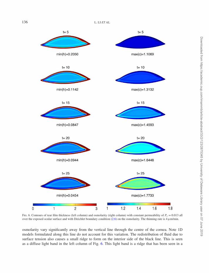
We begin by presenting results for the model with the same constant water permeability over the wholeocular surface; we use the corneal permeability corresponding to Pc = 0.013 measured by King-Smithet al. (2010b) and Bruhns et al. (2014). Figure 6 shows the contours of the simulation results. Theleft column represents the tear film thickness, and the right column represents the osmolarity. We seethe dark band (blue online) set inside of the boundary, representing the so-called black line, emergesrapidly near to and inside of the menisci in the left column. The black line develops due to capillaryaction resulting from the positive curvature of the menisci generating a low pressure that sucks fluidinto the meniscus. A local minimum thus forms near the meniscus, and is referred to as the black line.In addition, the canthi in the 2D eye-shaped domain induce a second direction of curvature, creatingan even lower pressure that attracts fluid towards themselves. Therefore, the tear film near the twocanthi is often thinner than other parts of the black line. In this case, the global minimum is locatednear the nasal canthus, which is sharper (more curved) than the temporal canthus. The formation ofthe global minimum is also promoted by the efflux of fluid near the nasal canthus due to the boundaryconditions that mimic punctal drainage from this region. This also shows that both the thickness and
135
Dow
nloaded from https://academ
ic.oup.com/im
amm
b/article-abstract/33/2/123/2875345 by University of D
elaware Library user on 07 June 2019
L. LI ET AL.
Fig. 6. Contours of tear film thickness (left column) and osmolarity (right column) with constant permeability of Pc = 0.013 allover the exposed ocular surface and with Dirichlet boundary condition (2.6) on the osmolarity. The thinning rate is 4 µm/min.
osmolarity vary significantly away from the vertical line through the centre of the cornea. Note 1Dmodels formulated along this line do not account for this variation. The redistribution of fluid due tosurface tension also causes a small ridge to form on the interior side of the black line. This is seenas a diffuse light band in the left column of Fig. 6. This light band is a ridge that has been seen in a
136
Dow
nloaded from https://academ
ic.oup.com/im
amm
b/article-abstract/33/2/123/2875345 by University of D
elaware Library user on 07 June 2019

COMPUTED TEAR FILM AND OSMOLARITY DYNAMICS ON AN EYE-SHAPED DOMAIN
−0.5 0 0.5 10.2
0.4
0.6
0.8
1
(a) (b)
y
t=5,10,15,20,25
h
−0.5 0 0.5 11
1.5
2
y
t=5,10,15,20,25
c
Fig. 7. Cross-sectional plots through the vertical line x = 0 with Pc = 0.013 and Dirichlet boundary condition (2.6). The thinningrate is 4 µm/min and the upper eyelid is located on the positive side of the y-axis. (a) Tear film thickness. (b) Osmolarity.
number of other studies (Maki et al., 2010a,b; Li et al., 2014). The tear film thickness in the interiordecreases steadily throughout the computation because of evaporation; this is visualized by the continualdarkening of the interior in the contour plots.
The corresponding osmolarity contours are plotted in the right column of Fig. 6. Generally, theosmolarity increases more where the tear film is thinner, such as in the black line and canthi regions.This is in qualitative agreement with the results of Zubkov et al. (2012); we return to a direct comparisonwith their 1D results for Pc = 0 in the next section. The global maximum of osmolarity is in the nasalcanthus that corresponds to the location of thinnest tear film. In the osmolarity plots, we observe abright band indicating that a region of elevated osmolarity is forming near the developing black line.Osmolarity in the interior continues to increase as a result of evaporation, and the interior of the eye-shaped domain becomes brighter in the plots. In the region where the tear film forms a small ridge,a corresponding darker band is also present on the interior side of the brighter band in the osmolarityplots.
The vertical cross-sectional plots (x = 0), shown in Fig. 7, illustrate more directly the correlationbetween the tear film thickness and osmolarity: the osmolarity is roughly the reciprocal of the tearfilm thickness except in the black line and meniscus regions. Furthermore, comparison with the zeropermeability case in the next section also reveals the effects of osmosis: the tear film is slightly thickerwhile the osmolarity is obviously smaller for the constant non-zero permeability case.
4.2 Zero permeability
Now, we consider our model on an impermeable ocular surface, i.e. Pc = 0, so as to reveal the effect ofosmosis by comparing with the previous results in Section 4.1, and we make comparisons with existingstudies on 1D domains to show that our model provides consistent predictions. In this case, no water issupplied in response to the increased osmolarity that occurs when water evaporates from the tear film.Figure 8 shows the contours of both tear film thickness and osmolarity on the eye-shaped domain att = 25. It shows that both the thickness and osmolarity vary significantly away from the vertical linethrough the centre of the cornea. For example, the global minimum of tear film thickness is located inthe nasal canthus and is much smaller than that in the cross-sectional plot. Furthermore, there is a spikein the osmolarity contour with a global maximum as large as max(c) = 4.8031 in the nasal canthus.These global extrema and their locations cannot be found via 1D models, and to our knowledge arenot available from clinical measurements either. From Fig. 8, we also see more elevated osmolarity atthe black line region, and the lowest concentration is located near the lacrimal gland as a result of thefresh tear supply. The tear film dynamics predicted by this model are in agreement with previous results(Li et al., 2014).
137
Dow
nloaded from https://academ
ic.oup.com/im
amm
b/article-abstract/33/2/123/2875345 by University of D
elaware Library user on 07 June 2019

L. LI ET AL.
Fig. 8. Contours of tear film thickness (left) and osmolarity (right) with Pc = 0 and Dirichlet boundary condition (2.6). Thethinning rate is 4 µm/min.
Table 3 Extreme values for various cases; Pc(x, y) denotes the variable permeability case and is givenby Equation (2.3).
Thinning rate: 4 µm/min 10 µm/min 20 µm/min
Pc = 0 Pc = 0.013 Pc(x, y) Pc(x, y) Pc(x, y)
min(h(x, y, 5)) 0.2043 0.2050 0.2070 0.1880 0.1557min(h(x, y, 10)) 0.1072 0.1142 0.1294 0.1102 0.0931min(h(x, y, 15)) 0.0819 0.0847 0.0899 0.0722 0.0506min(h(x, y, 20)) 0.0716 0.0944 0.1118 0.0906 0.0471min(h(x, y, 25)) 0.0343 0.0454 0.0492 0.0382 0.0268
max(c(x, y, 5)) 1.1135 1.1069 1.0873 1.2392 1.5629max(c(x, y, 10)) 1.3925 1.3132 1.1722 1.5091 2.7505max(c(x, y, 15)) 1.6975 1.4593 1.2673 1.9892 5.3456max(c(x, y, 20)) 2.4841 1.6448 1.3852 2.6045 5.9684max(c(x, y, 25)) 4.8031 1.7733 1.5124 3.1486 6.0538
The effect of osmosis can be readily seen by comparing the extreme values of different perme-ability cases. The extreme values of both h and c for several cases we considered in this paper arelisted in Table 3. For the constant non-zero permeability case (Pc = 0.013), the minimum thickness(min(h) = 0.0454) is slightly larger than that with zero permeability (min(h) = 0.0343) at t = 25. How-ever, the peak of osmolarity is significantly reduced by osmotic flows: max(c) = 1.7733 with constantpermeability and max(c) = 4.8031 with zero permeability at t = 25. Therefore, according to our compu-tation, we conclude that the presence of osmotic flux across the corneal surface may protect the tear filmfrom excessive hyperosmolarity which could cause damage to the ocular surface and/or denaturation oftear film mucins and proteins (Govindarajan & Gipson, 2010).
Zubkov et al. (2012) studied a system that included both tear film and osmolarity dynamics on a1D domain with a moving end that mimicked blinks; their model assumes that the ocular surface isimpermeable. To compare with their model, we set Pc = 0 and show the cross-sectional plots throughthe vertical line x = 0; the results are in Fig. 9. The cross-sectional curves of our results on the 2Deye-shaped domain are comparable to the 1D results of Zubkov et al. (2012) during the interblinkphase for both the tear film thickness (Fig. 9a) and the osmolarity distribution (Fig. 9b), except that thedevelopment of the black line is slower and the maximum osmolarity is higher in our results. The slowerdevelopment of the black line in our results is due to the stationary domain, because the formation ofthe black line begins during the opening phase according to previous results on 1D blinking domains
138
Dow
nloaded from https://academ
ic.oup.com/im
amm
b/article-abstract/33/2/123/2875345 by University of D
elaware Library user on 07 June 2019
COMPUTED TEAR FILM AND OSMOLARITY DYNAMICS ON AN EYE-SHAPED DOMAIN
−0.5 0 0.5 10.2
0.4
0.6
0.8
1(a) (b)
y
t=5,10,15,20,25
h
−0.5 0 0.5 11
1.5
2
y
t=5,10,15,20,25
c
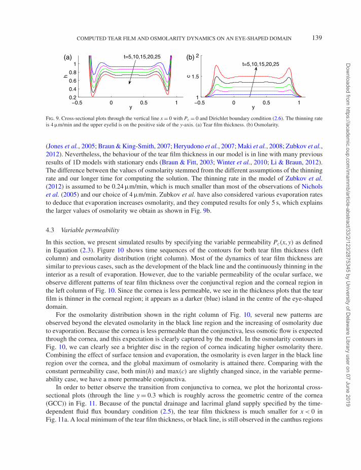
Fig. 9. Cross-sectional plots through the vertical line x = 0 with Pc = 0 and Dirichlet boundary condition (2.6). The thinning rateis 4 µm/min and the upper eyelid is on the positive side of the y-axis. (a) Tear film thickness. (b) Osmolarity.
(Jones et al., 2005; Braun & King-Smith, 2007; Heryudono et al., 2007; Maki et al., 2008; Zubkov et al.,2012). Nevertheless, the behaviour of the tear film thickness in our model is in line with many previousresults of 1D models with stationary ends (Braun & Fitt, 2003; Winter et al., 2010; Li & Braun, 2012).The difference between the values of osmolarity stemmed from the different assumptions of the thinningrate and our longer time for computing the solution. The thinning rate in the model of Zubkov et al.(2012) is assumed to be 0.24 µm/min, which is much smaller than most of the observations of Nicholset al. (2005) and our choice of 4 µm/min. Zubkov et al. have also considered various evaporation ratesto deduce that evaporation increases osmolarity, and they computed results for only 5 s, which explainsthe larger values of osmolarity we obtain as shown in Fig. 9b.
4.3 Variable permeability
In this section, we present simulated results by specifying the variable permeability Pc(x, y) as definedin Equation (2.3). Figure 10 shows time sequences of the contours for both tear film thickness (leftcolumn) and osmolarity distribution (right column). Most of the dynamics of tear film thickness aresimilar to previous cases, such as the development of the black line and the continuously thinning in theinterior as a result of evaporation. However, due to the variable permeability of the ocular surface, weobserve different patterns of tear film thickness over the conjunctival region and the corneal region inthe left column of Fig. 10. Since the cornea is less permeable, we see in the thickness plots that the tearfilm is thinner in the corneal region; it appears as a darker (blue) island in the centre of the eye-shapeddomain.
For the osmolarity distribution shown in the right column of Fig. 10, several new patterns areobserved beyond the elevated osmolarity in the black line region and the increasing of osmolarity dueto evaporation. Because the cornea is less permeable than the conjunctiva, less osmotic flow is expectedthrough the cornea, and this expectation is clearly captured by the model. In the osmolarity contours inFig. 10, we can clearly see a brighter disc in the region of cornea indicating higher osmolarity there.Combining the effect of surface tension and evaporation, the osmolarity is even larger in the black lineregion over the cornea, and the global maximum of osmolarity is attained there. Comparing with theconstant permeability case, both min(h) and max(c) are slightly changed since, in the variable perme-ability case, we have a more permeable conjunctiva.
In order to better observe the transition from conjunctiva to cornea, we plot the horizontal cross-sectional plots (through the line y = 0.3 which is roughly across the geometric centre of the cornea(GCC)) in Fig. 11. Because of the punctal drainage and lacrimal gland supply specified by the time-dependent fluid flux boundary condition (2.5), the tear film thickness is much smaller for x < 0 inFig. 11a. A local minimum of the tear film thickness, or black line, is still observed in the canthus regions
139
Dow
nloaded from https://academ
ic.oup.com/im
amm
b/article-abstract/33/2/123/2875345 by University of D
elaware Library user on 07 June 2019

L. LI ET AL.
Fig. 10. Contours of tear film thickness (left column) and osmolarity (right column) with variable permeability (2.3) and Dirichletboundary condition (2.6). The thinning rate is 4 µm/min.
due to the curvature of the menisci. The abrupt change of permeability from conjunctiva to cornea isreflected by the tear film thickness. In Fig. 11a, we see a rapid drop of tear film thickness around x = ±1near the boundary of the cornea. The transition of permeability influences the osmolarity distribution
140
Dow
nloaded from https://academ
ic.oup.com/im
amm
b/article-abstract/33/2/123/2875345 by University of D
elaware Library user on 07 June 2019
COMPUTED TEAR FILM AND OSMOLARITY DYNAMICS ON AN EYE-SHAPED DOMAIN
−3 −2 −1 0 1 2 3
0.20.40.60.8
1
x
t=5,10,15,20,25
h
−3 −2 −1 0 1 2 31
1.2
1.4t=5,10,15,20,25
x
c
(a) (b)
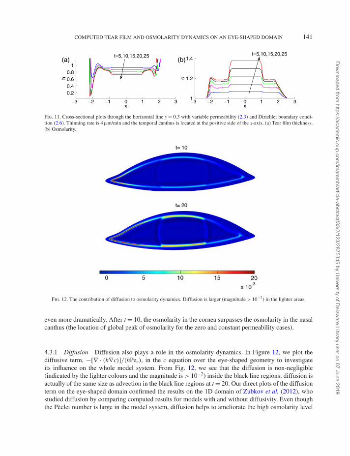
Fig. 11. Cross-sectional plots through the horizontal line y = 0.3 with variable permeability (2.3) and Dirichlet boundary condi-tion (2.6). Thinning rate is 4 µm/min and the temporal canthus is located at the positive side of the x-axis. (a) Tear film thickness.(b) Osmolarity.
Fig. 12. The contribution of diffusion to osmolarity dynamics. Diffusion is larger (magnitude > 10−2) in the lighter areas.
even more dramatically. After t = 10, the osmolarity in the cornea surpasses the osmolarity in the nasalcanthus (the location of global peak of osmolarity for the zero and constant permeability cases).
4.3.1 Diffusion Diffusion also plays a role in the osmolarity dynamics. In Figure 12, we plot thediffusive term, −[∇ · (h∇c)]/(hPec), in the c equation over the eye-shaped geometry to investigateits influence on the whole model system. From Fig. 12, we see that the diffusion is non-negligible(indicated by the lighter colours and the magnitude is > 10−2) inside the black line regions; diffusion isactually of the same size as advection in the black line regions at t = 20. Our direct plots of the diffusionterm on the eye-shaped domain confirmed the results on the 1D domain of Zubkov et al. (2012), whostudied diffusion by comparing computed results for models with and without diffusivity. Even thoughthe Pèclet number is large in the model system, diffusion helps to ameliorate the high osmolarity level
141
Dow
nloaded from https://academ
ic.oup.com/im
amm
b/article-abstract/33/2/123/2875345 by University of D
elaware Library user on 07 June 2019

L. LI ET AL.
Fig. 13. Fluid flux (Q) over contours of its magnitude with variable permeability and thinning rate 4 µm/min. (Far fewer arrowsthan the computational grid points are shown for clarity. All the arrows in this plot start at different locations.)
in the black line regions. Diffusion could affect the osmolarity distribution similarly in local spots ofbreak-up (Peng et al., 2014).
4.3.2 Movement of fluid and solutes Figure 13 shows the quiver plots of the fluid flux Q at timet = 1 and t = 20. The normalized arrows in the plots show the directions only, and we use the shading toindicate the magnitude of the flux vector: the darker the background, the smaller is the flux. In particular,white indicates a flux > 10−2; dark grey is < 10−3. At t = 1, the formation of the black line dominatesthe movement of tear fluid. We see from the first plot of Fig. 13 that relatively fast flow (‖Q‖ � 10−2)is observed near the menisci, and all the arrows pointing towards the eye lids. This is because the lowerpressure created by the menisci attracts the nearby fluid forming a locally thin region. This thin regionis referred to as the black line and corresponds to the dark blue band as we pointed out in the thicknesscontour plots previously. In the second plots of Fig. 13, relatively fast fluid motion (‖Q‖ � 10−2) stilloccurs in the menisci; however, the arrows in the menisci show that the flow splits near the lacrimalgland and moves towards the nasal canthus along the eye lids. This hydraulic connectivity is thought tobe caused by the pressure difference created by the time-dependent influx and efflux on the boundary.The pressure gradient in the menisci drives the fluid flows towards the nasal side.
Li et al. (2014) have studied tear flow over the eye-shaped geometry specifying the same time-dependent flux BC (2.5). They discovered that, after the development of the black line, relatively fastfluid flow occurs in the menisci corresponding to the experimentally observed hydraulic connectivity,while, on the inner side of the black line region, fluid flow is small. The model in this paper couples thefluid dynamics in the tear film with the osmolarity and still captures hydraulic connectivity.
The model Equations (2.1) and (2.2) can be combined into a single PDE (Peng et al., 2014):
∂t(ch) + ∇ ·(
cQ − h
Pec∇c
)= 0. (4.1)
142
Dow
nloaded from https://academ
ic.oup.com/im
amm
b/article-abstract/33/2/123/2875345 by University of D
elaware Library user on 07 June 2019

COMPUTED TEAR FILM AND OSMOLARITY DYNAMICS ON AN EYE-SHAPED DOMAIN
Fig. 14. Contour for c(x, y, t)h(x, y, t) − c(x, y, 0)h(x, y, 0) with variable permeability and thinning rate 4 µm/min.
Here ch represents the mass per unit area of the solute. From this equation, we see that the solute wouldmove with fluid flow, ∇ · (cQ), and would diffuse from a higher concentration to lower concentration∇ · (−h∇c)/Pec. However, since we have a very large Péclet number for the osmolarity, we expect thesolute to move primarily with the fluid flow. Figure 14 shows the contours of the change of the massper area as opposed to its initial condition: c(x, y, t)h(x, y, t) − c(x, y, 0)h(x, y, 0). The left plot of Fig. 14shows the redistribution of the solute at t = 1. We see a decrease of mass in the black line region andincrease of mass in the menisci corresponding to the formation of the black line; it matches with fluidmovement as shown in Fig. 13. At t = 20, the redistribution of mass (right plot of Fig. 14) also matchesthe fluid motion; the increase of solute mass corresponds to the influx from the lacrimal gland, andsubsequent flow around the meniscus. The decreases can be explained by the drainage that occurred atthe puncta. Another interesting point we note from Fig. 14 is that variable permeability does not have aneffect on ch, because Equation (4.1) does not depend on permeability at all. In general, solutes in the tearfluid move mostly with the fluid flow. Throughout the time considered, the change of c(x, y, t)h(x, y, t)is rather small in the interior, and thus the reciprocal relation between c and h generally holds in theinterior eye.
4.4 Increased evaporation rate
The average thinning rate for the pre-corneal tear film (PCTF) measured by Nichols et al. (2005) is3.79 ± 4.20 µm/min, with the fastest observed PCTF thinning rate being 20 µ/min. We attempt to inves-tigate how evaporation influences tear film and osmolarity dynamics by adjusting the parameters thatcorrespond to an increased thinning rate of 20 µm/min.
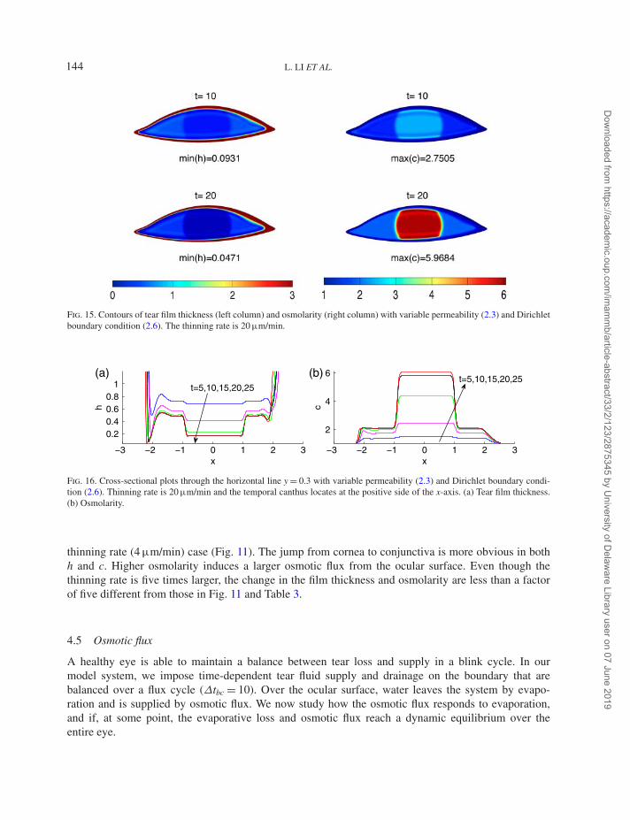
Figure 15 shows the contours of both h(x, y, t) and c(x, y, t) with parameters specified such that thethinning rate for a flat film is 20 µm/min and with variable permeability. Compared with the previousresults for the normal thinning rate (4 µm/min), we observe the following effects deduced by elevatedevaporation. In the thickness contour plots, we observe that the black line forms more rapidly, theinterior tear film thickness decreases faster to a thinner level, the global minimum is smaller and thetransition from conjunctiva to cornea is more obvious. The associated osmolarity contours indicate thatthe osmolarity is more elevated with a larger global maximum value than the previous 4 µm/min case.Moreover, the osmolarity difference between cornea and conjunctiva is more pronounced. In addition,we can see that the tear film thins faster with higher evaporation by comparing the extreme values listedin Table 3. We deduce that evaporation increases osmolarity, confirming the 1D results of Zubkov et al.(2012).
The horizontal cross-sectional plots shown in Fig. 16 give another view of the tear film thicknessand osmolarity, as well as their correlation. Clearly, the tear film becomes much thinner and osmolarityis much more elevated, especially over the corneal region (roughly −1 � x � 1) than with the normal
143
Dow
nloaded from https://academ
ic.oup.com/im
amm
b/article-abstract/33/2/123/2875345 by University of D
elaware Library user on 07 June 2019
L. LI ET AL.
Fig. 15. Contours of tear film thickness (left column) and osmolarity (right column) with variable permeability (2.3) and Dirichletboundary condition (2.6). The thinning rate is 20 µm/min.
−3 −2 −1 0 1 2 3
0.20.40.60.8
1
x
t=5,10,15,20,25
h
−3 −2 −1 0 1 2 3
2
4
6t=5,10,15,20,25
x
c
(a) (b)
Fig. 16. Cross-sectional plots through the horizontal line y = 0.3 with variable permeability (2.3) and Dirichlet boundary condi-tion (2.6). Thinning rate is 20 µm/min and the temporal canthus locates at the positive side of the x-axis. (a) Tear film thickness.(b) Osmolarity.
thinning rate (4 µm/min) case (Fig. 11). The jump from cornea to conjunctiva is more obvious in bothh and c. Higher osmolarity induces a larger osmotic flux from the ocular surface. Even though thethinning rate is five times larger, the change in the film thickness and osmolarity are less than a factorof five different from those in Fig. 11 and Table 3.
4.5 Osmotic flux
A healthy eye is able to maintain a balance between tear loss and supply in a blink cycle. In ourmodel system, we impose time-dependent tear fluid supply and drainage on the boundary that arebalanced over a flux cycle (Δtbc = 10). Over the ocular surface, water leaves the system by evapo-ration and is supplied by osmotic flux. We now study how the osmotic flux responds to evaporation,and if, at some point, the evaporative loss and osmotic flux reach a dynamic equilibrium over theentire eye.
144
Dow
nloaded from https://academ
ic.oup.com/im
amm
b/article-abstract/33/2/123/2875345 by University of D
elaware Library user on 07 June 2019

COMPUTED TEAR FILM AND OSMOLARITY DYNAMICS ON AN EYE-SHAPED DOMAIN
0 5 10 15 20 250
0.1
0.2
0.3
0.4Osmotic Flux vs. Evaporation
t
Vol
umet
ric F
lux
Osmotic Flux
Evaporation
0 5 10 15 20 250
0.2
0.4
0.6
0.8Osmotic Flux vs. Evaporation
t
Vol
umet
ric F
lux
Osmotic Flux
Evaporation
(a) (b)
Fig. 17. Competition between evaporative loss and osmotic flux (volume/time). (a) Thinning rate is 20 µm/min. (b) Thinning rateis 38 µm/min.
To evaluate the volumetric flux of evaporation and osmosis, we integrate the PDE (2.1) over theeye-shaped domain Ω and find:
volumetric flux of evaporation: Fe(t) =∫∫
Ω
EJ dA,
volumetric flux of osmosis: Fo(t) =∫∫
Ω
Pc(c − 1) dA.
We plot Fe(t) and Fo(t) together in Fig. 17 to investigate the competition between evaporation and osmo-sis over the eye-shaped domain. Both plots in Fig. 17 are simulation results with variable permeability,but with different thinning rates. Note that 38 µm/min is the thinning rate of the bare water interface(Peng et al., 2014). As is seen in the plots, osmotic flux is induced immediately in the simulations. Theosmotic flux increases much faster with the higher thinning rate (38 µm/min), and is seen to reach anequilibrium after t = 15. The volumetric flux of evaporation stays almost constant for the 20 µm/mincase, while a slight decrease is observed for the 38 µm/min case. Faster evaporation makes the tear filmthin faster, and reach the equilibrium thickness at more locations on the eye. The presence of van derWaals forces prevents the tear film from completely dewetting the ocular surface, and evaporation isshut off when and where a very thin equilibrium h is reached. This results in a decrease of volumetricflux of evaporation over the entire eye. We believe that ultimately the evaporation and osmosis wouldbalance each other and the system would achieve a dynamic equilibrium. However, we cannot verifythis because the pressure gradient inside the tear film, between the meniscus and the interior, becomestoo steep for our current numerical methods to accurately resolve after t = 25. Similar issues limited theamount of time that could be computed in previous models as well (Maki et al., 2010a,b; Li et al., 2014).We also doubt that the equilibrium between evaporation and osmosis can be observed in experimentsbecause, before the equilibrium is reached, reflex tearing and/or blinks are more likely induced whenthe osmolarity level is high enough.
4.6 Neumann boundary condition for the osmolarity
We also consider the homogeneous Neumann boundary condition (2.7) for our system. It specifiesno flux for osmolarity on the boundary; that is, solute cannot pass through the boundary. The com-puted results with this Neumann boundary condition (2.7) is rather similar to previous results using theDirichlet boundary condition (2.6). This is because there is a large amount of fluid in the menisci and thefluid interaction between the menisci and interior is small due to the presence of the black line separating
145
Dow
nloaded from https://academ
ic.oup.com/im
amm
b/article-abstract/33/2/123/2875345 by University of D
elaware Library user on 07 June 2019
L. LI ET AL.
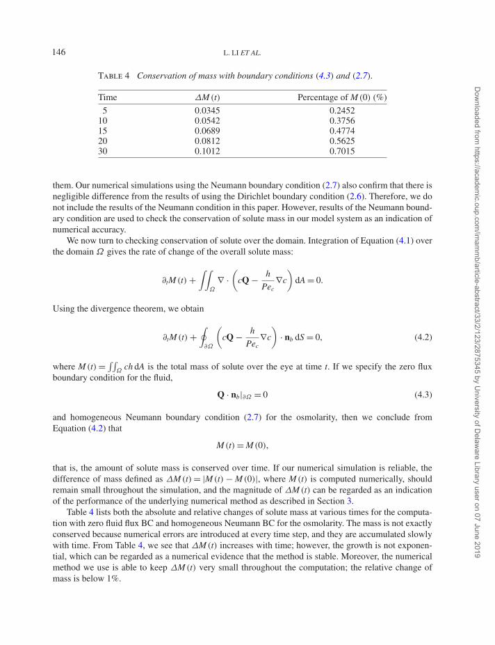
Table 4 Conservation of mass with boundary conditions (4.3) and (2.7).
Time ΔM (t) Percentage of M (0) (%)
5 0.0345 0.245210 0.0542 0.375615 0.0689 0.477420 0.0812 0.562530 0.1012 0.7015
them. Our numerical simulations using the Neumann boundary condition (2.7) also confirm that there isnegligible difference from the results of using the Dirichlet boundary condition (2.6). Therefore, we donot include the results of the Neumann condition in this paper. However, results of the Neumann bound-ary condition are used to check the conservation of solute mass in our model system as an indication ofnumerical accuracy.
We now turn to checking conservation of solute over the domain. Integration of Equation (4.1) overthe domain Ω gives the rate of change of the overall solute mass:
∂tM (t) +∫∫
Ω
∇ ·(
cQ − h
Pec∇c
)dA = 0.
Using the divergence theorem, we obtain
∂tM (t) +∮
∂Ω
(cQ − h
Pec∇c
)· nb dS = 0, (4.2)
where M (t) = ∫∫Ω
ch dA is the total mass of solute over the eye at time t. If we specify the zero fluxboundary condition for the fluid,
Q · nb|∂Ω = 0 (4.3)
and homogeneous Neumann boundary condition (2.7) for the osmolarity, then we conclude fromEquation (4.2) that
M (t) = M (0),
that is, the amount of solute mass is conserved over time. If our numerical simulation is reliable, thedifference of mass defined as ΔM (t) = |M (t) − M (0)|, where M (t) is computed numerically, shouldremain small throughout the simulation, and the magnitude of ΔM (t) can be regarded as an indicationof the performance of the underlying numerical method as described in Section 3.
Table 4 lists both the absolute and relative changes of solute mass at various times for the computa-tion with zero fluid flux BC and homogeneous Neumann BC for the osmolarity. The mass is not exactlyconserved because numerical errors are introduced at every time step, and they are accumulated slowlywith time. From Table 4, we see that ΔM (t) increases with time; however, the growth is not exponen-tial, which can be regarded as a numerical evidence that the method is stable. Moreover, the numericalmethod we use is able to keep ΔM (t) very small throughout the computation; the relative change ofmass is below 1%.
146
Dow
nloaded from https://academ
ic.oup.com/im
amm
b/article-abstract/33/2/123/2875345 by University of D
elaware Library user on 07 June 2019

COMPUTED TEAR FILM AND OSMOLARITY DYNAMICS ON AN EYE-SHAPED DOMAIN
5. Conclusion
The mathematical model in this paper combines tear film flow, evaporation, osmolarity and osmosis onan eye-shaped domain representing the exposed ocular surface. To our knowledge, this is the first suchmodel that includes the osmolarity in a 2D tear film model. The results give information that we believeis not available from human subjects or animal models of the tear film. We believe that these resultshelp give context to osmolarity measurements in vivo (e.g. Benelli et al., 2010; Lemp et al., 2011). Theresults show that the location and value of the minimum tear film thickness and maximum osmolarityare found to be sensitive to the permeability at the tear/eye interface.
Measurements of tear film osmolarity in human subjects are made from the inferior meniscus, ormore commonly, near the temporal canthus. These measurements have been calibrated with respect toDES so that diagnosis of DES is possible with better single-measurement specificity and sensitivitythan other single signs or symptoms of DES (Gilbard et al., 1978; Lemp et al., 2011; Sullivan, 2014).When used for those purposes, the meniscal osmolarity measurement accomplishes its aim, but occa-sionally some investigators will try to infer osmolarity values in other parts of the tear film. But arethose meniscus or canthus measurements informative about what is going on in the dynamics of therest of the tear film? The values in the interior are quite different from those in the meniscus near thetemporal canthus according to our model. For low evaporation rates of 1 micron/min or less, our resultsare similar to those of Zubkov et al. (2012), with modest increases of osmolarity away from meniscusand particularly in the black line. For larger evaporation rates and longer interblink times, such as thosethat may be encountered in clinical experiments, our results indicate higher osmolarities. With variablepermeability as suggested by experimental measurement (King-Smith et al., 2010b), we find that, for4 µm/min thinning rates, the peak value of the osmolarity increases to 51% over the isotonic value, orabout 457 Osm/m3. This is just at the edge of sensory detection according to the results of Liu et al.(2009), assuming that there is no neuropathy present that would reduce sensory perception at the ocu-lar surface. For 10 and 20 µm/min thinning rates (Nichols et al., 2005; King-Smith et al., 2010a), weobtain maximum values of 951 and 1828 Osm/m3, respectively; these values are quite high comparedwith what is mentioned for meniscus measurements reported in the literature, and would certainly befelt by subjects with normal neural function (Liu et al., 2009). For all of these cases, the maximumoccurs in the black line over the cornea. For the current model, there is very little change in the osmo-larity in the outer canthus, which would make it difficult to use that location to deduce the differentmaxima in the osmolarity. The variability in the osmolarity in the meniscus as measured clinically islikely due to mixing of the tear film due to blinking (Lemp et al., 2011; Sullivan, 2014), which is notincluded in the present model.
There are some additional limitations to the current study for linking the osmolarity measured invivo with the computed results. (i) As previously mentioned, there is no lid motion to mix the tearfluid as occurs in vivo, which contributes to the variability observed in vivo. (ii) Once the black line isformed in the computed results, there is little exchange between the tear film in the interior with themeniscus. The supply and drainage of tear fluid occurs in and affects primarily the meniscus, and thistends to hold the meniscal values of the osmolarity close to the isotonic value. (iii) The volume of tearfluid is probably large compared with that of DES subjects, and could affect the values of osmolarityobtained. (iv) The model does not include break-up per se, and there have been results that suggestthat the osmolarity could be quite high in these localized regions (e.g. Liu et al., 2009; Braun et al.,2010; King-Smith et al., 2010b; Braun, 2012; Peng et al., 2014). These points suggest possible fruitfuldirections for future research. Additional directions would include a dynamic lipid layer that affects theevaporation rate in a sensible way on the eye-shaped domain; possible models are those of Bruna &Breward (2014) and Peng et al. (2014).
147
Dow
nloaded from https://academ
ic.oup.com/im
amm
b/article-abstract/33/2/123/2875345 by University of D
elaware Library user on 07 June 2019

L. LI ET AL.
Funding
This material is based upon work supported by the National Science Foundation under GrantNo. 1022706 (L.L., R.J.B., T.A.D.) and the National Institutes of Health R01-EY017951 (P.E.K.S.).L.L. and R.J.B. were partially supported by the Institute for Mathematics and its Applications at theUniversity of Minnesota during the completion of this work.
Note Added in Press
During publication of this paper, a reference for the permeabilities appeared: Braun, R. J., King-Smith,P. E., Begley, C. G., Li, Longfei and Gewecke, N. R. (2015) Dynamics and function of the tear film inrelation to the blink cycle. Prog. Ret. Eye Res. 45, 132–164.
References
Ajaev, V. S. & Homsy, G. (2001) Steady vapor bubbles in rectangular microchannels. J. Colloid Interface Sci.,240, 259–271.
Amparo, F., Hamrah, P., Schaumberg, D. A. & Dana, R. (2014) The value of tear osmolarity as a metricin evaluating the response to dry eye therapy in the clinic and in clinical trials. Am. J. Ophthalmol., 157,915–916.
Amparo, F., Jin, Y., Hamrah, P., Schaumberg, D. A. & Dana, R. (2013) What is the value of incorporating tearosmolarity measurement in assessing patient response to therapy in dry eye disease? Am. J. Ophthalmol., 157,69–77.e2.
Anonymous (2007) Report of the international dry eye workshop (DEWS). Ocul. Surf., 5, 65–204.Baudouin, C., Aragona, P., Messmer, E. M., Tomlinson, A., Calonge, M., Boboridis, K. G., Akova, Y. A.,
Geerling, G., Labetoulle, M. & Rolando, M. (2013) Role of hyperosmolarity in the pathogenesis andmanagement of dry eye disease: proceedings of the ocean group meeting. Ocul. Surf., 11, 246–258.
Benelli, U., Nardi, M., Posarelli, C. & Albert, T. G. (2010) Tear osmolarity measurement using the TearLabTM
osmolarity system in the assessment of dry eye treatment effectiveness. Contact Lens Anterior Eye, 33,61–67.
Berger, R. E. & Corrsin, S. (1974) A surface tension gradient mechanism for driving the pre-corneal tear filmafter a blink. J. Biomech., 7, 225–228.
Braun, R. J. (2012) Dynamics of the tear film. Annu. Rev. Fluid Mech., 44, 267–297.Braun, R. J. & Fitt, A. D. (2003) Modeling the drainage of the pre-corneal tear film after a blink. Math. Med.
Biol., 20, 1–28.Braun, R. J., Gewecke, N., Begley, C. G., King-Smith, P. E. & Siddique, J. I. (2014) A model for tear film
thinning with osmolarity and fluorescein. Invest. Ophthalmol. Vis. Sci., 55, 1133–1142.Braun, R. J. & King-Smith, P. E. (2007) Model problems for the tear film in a blink cycle: single equation models.
J. Fluid Mech., 586, 465–490.Braun, R. J., King-Smith, P. E., Nichols, J. J. & Ramamoorthy, P. (2010) On computational models for tear film
and osmolarity dynamics. 6th International Conference on the Tear Film and Ocular Surface: Basic Scienceand Clinical Relevance, Poster 46 (abstract).
Braun, R. J., Usha, R., McFadden, G. B., Driscoll, T. A., Cook, L. P. & King-Smith, P. E. (2012) Thin filmdynamics on a prolate spheroid with application to the cornea. J. Eng. Math., 73, 121–138.
Brenan, K. E., Campbell, S. L. & Petzold, L. R. (1996) Numerical Solution of Initial-Value Problems inDifferential-Algebraic Equations. Philadelphia: SIAM.
Bron, A., Tiffany, J., Gouveia, S., Yokoi, N. & Voon, L. (2004) Functional aspects of the tear film lipid layer.Exp. Eye Res., 78, 347–360.
148
Dow
nloaded from https://academ
ic.oup.com/im
amm
b/article-abstract/33/2/123/2875345 by University of D
elaware Library user on 07 June 2019
COMPUTED TEAR FILM AND OSMOLARITY DYNAMICS ON AN EYE-SHAPED DOMAIN
Bruhns, J. L., Braun, R. J., Evans, R. M., Freeman, D. B., King-Smith, P. E., Ramamoorthy, P. & Nichols,J. J. (2014) Models for interaction of the tear film with the corneal and conjunctival epithelia (in preparation).
Bruna, M. & Breward, C. J. W. (2014) The influence of nonpolar lipids on tear film dynamics. J. Fluid Mech.,746, 565–605.
Chesshire, G. & Henshaw, W. D. (1990) Composite overlapping meshes for the solution of partial differentialequations. J. Comput. Phys., 90, 1–64.
Dartt, D. A. (2002) Regulation of mucin and fluid secretion by conjunctival epithelial cells. Prog. Ret. Eye Res.,21, 555–576.
Dartt, D. A. (2009) Neural regulation of lacrimal gland secretory processes: relevance in dry eye diseases.Prog. Ret. Eye Res, 28, 155–177.
Dartt, D. A., Hodges, R. R. & Zoukhri, D. (2005) Tears and their secretion. The Biology of the Eye (J. Fischbarged.). Advances in Organ Biology, vol. 10. Amsterdam: Elsevier, pp. 21–82.
Deng, Q., Braun, R. J. & Driscoll, T. A. (2014) Heat transfer and tear film dynamics over multiple blink cycles.Phys. Fluids, 26, 071901.
Deng, Q., Driscoll, T. A., Braun, R. J. & King-Smith, P. E. (2013) A model for the tear film and ocular surfacetemperature for partial blinks. Interfacial Phen. Ht. Trans., 1, 357–381.
Doane, M. (1989) An instrument for in vivo tear film interferometry. Optom. Vis. Sci., 66, 383–388.Doane, M. G. (1981) Blinking and the mechanics of the lacrimal drainage system. Ophthalmology, 88, 844–851.Efron, N., Young, G. & Brennan, N. A. (1989) Ocular surface temperature. Curr. Eye. Res., 8, 901–906.Gilbard, J. P., Farris, R. L. & Santamaria, J. (1978) Osmolarity of tear microvolumes in keratoconjunctivitis
sicca. Arch. Ophthalmol., 96, 677–681.Gipson, I. K. (2004) Distribution of mucins at the ocular surface. Exp. Eye Res., 78, 379–388.Golding, T. R., Bruce, A. S. & Mainstone, J. C. (1997) Relationship between tear-meniscus parameters and
tear-film breakup. Cornea, 16, 649–661.Govindarajan, B. & Gipson, I. (2010) Membrane-tethered mucins have multiple functions on the ocular surface.
Exp. Eye Res., 90, 655–693.Harrison, W. W., Begley, C. G., Liu, H., Chen, M., Garcia, M. & Smith, J. A. (2008) Menisci and fullness of
the blink in dry eye. Optom. Vis. Sci., 85, 706–714.Henshaw, W. D. (2002) Ogen: the overture overlapping grid generator. Technical Report UCRL-MA-132237.
Lawrence Livermore National Laboratory.Heryudono, A., Braun, R. J., Driscoll, T. A., Cook, L. P., Maki, K. L. & King-Smith, P. E. (2007) Single-
equation models for the tear film in a blink cycle: realistic lid motion. Math. Med. Biol., 24, 347–377.Holly, F. (1973) Formation and rupture of the tear film. Exp. Eye Res., 15, 515–525.Jensen, O. E. & Grotberg, J. B. (1993) The spreading of heat or soluble surfactant along a thin liquid film.
Phys. Fluids A, 75, 58–68.Johnson, M. E. & Murphy, P. J. (2004) Changes in the tear film and ocular surface from dry eye syndrome.
Prog. Ret. Eye Res., 23, 449–474.Jones, M. B., McElwain, D. L. S., Fulford, G. R., Collins, M. J. & Roberts, A. P. (2006) The effect of the
lipid layer on tear film behavior. Bull. Math. Biol., 68, 1355–1381.Jones, M. B., Please, C. P., McElwain, D. L. S., Fulford, G. R., Roberts, A. P. & Collins, M. J. (2005)
Dynamics of tear film deposition and drainage. Math. Med. Bio., 22, 265–288.Jossic, L., Lefevre, P., de Loubens, C., Magnin, A. & Corre, C. (2009) The fluid mechanics of shear-thinning
tear substitutes. J. Non-Newton. Fluid Mech., 161, 1–9.Kimball, S. H., King-Smith, P. E. & Nichols, J. J. (2010) Evidence for the major contribution of evaporation to
tear film thinning between blinks. Invest. Opthalmol. Vis. Sci., 51, 6294–6297.King-Smith, P. E., Fink, B. A., Hill, R. M., Koelling, K. W. & Tiffany, J. M. (2004) The thickness of the tear
film. Curr. Eye. Res., 29, 357–368.King-Smith, P. E., Fink, B. A., Nichols, J. J., Nichols, K. K., Braun, R. J. & McFadden, G. B. (2009) The
contribution of lipid layer movement to tear film thinning and breakup. Invest. Ophthalmol. Visual Sci.,50, 2747–2756.
149
Dow
nloaded from https://academ
ic.oup.com/im
amm
b/article-abstract/33/2/123/2875345 by University of D
elaware Library user on 07 June 2019
L. LI ET AL.
King-Smith, P. E., Hinel, E. A. & Nichols, J. J. (2010a) Application of a novel interferometric method toinvestigate the relation between lipid layer thickness and tear film thinning. Invest. Ophthalmol. Vis. Sci., 51,2418–2423.
King-Smith, P. E., Nichols, J. J., Nichols, K. K. & Braun, R. J. (2011) A high resolution microscope for imagingthe lipid layer of the tear film. Ocul. Surf., 9, 197–211.
King-Smith, P. E., Nichols, J. J., Nichols, K. K., Fink, B. A., Green-Church, K. B. & Braun, R. J. (2007)Does the water permeability of the corneal surface help prevent excessive evaporative thinning of the tear film?5th International Conference on the Tear Film and Ocular Surface: Basic Science and Clinical Relevance,Taormina, Italy.
King-Smith, P. E., Ramamoorthy, P., Braun, R. J. & Nichols, J. J. (2013) Tear film images and breakup ana-lyzed using fluorescent quenching. Invest. Ophthalmol. Vis. Sci., 54, 6003–6011.
King-Smith, P. E., Ramamoorthy, P., Nichols, K. K., Braun, R. J. & Nichols, J. J. (2010b) If tear evaporationis so high, why is tear osmolarity so low? 6th International Conference on the Tear Film and Ocular Surface:Basic Science and Clinical Relevance, Poster 43 (abstract).
Lakowicz, J. R. (2006) Principal of Fluorescence Spectroscopy, 3rd edn. New York: Springer.Leiske, D. L., Leiske, C. I., Leiske, D. R., Toney, M. F., Senchyna, M., Ketelson, H. A., Meadows, D. L.
& Fuller, G. G. (2011) Temperature-induced transitions in the structure and interfacial rheology of humanmeibum. Biophys. J., 102, 369–376.
Leiske, D. L., Miller, C. E., Rosenfeld, L., Cerretani, C., Ayzner, A., Lin, B., Meron, M., Senchyna, M.,Ketelson, H. A., Meadows, D., Srinivasan, S., Jones, L., Radke, C. J., Toney, M. F. & Fuller, G. G.(2012) Molecular structure of interfacial human meibum films. Langmuir, 28, 11858–11865.
Lemp, M. A. (2007) The definition and classification of dry eye disease: report of the definition and classificationsubcommittee of the international dry eye workshop. Ocul. Surf., 5, 75–92.
Lemp, M. A., Bron, A. J. & Baudoin, C. (2011) Tear osmolarity in the diagnosis and management of dry eyedisease. Am. J. Ophthalmol., 151, 792–798.
Levin, M. H. & Verkman, A. S. (2004) Aquaporin-dependent water permeation at the mouse ocular sur-face: in vivo microfluorometric measurements in cornea and conjunctiva. Invest. Ophthalmol. Vis. Sci., 45,4423–4432.
Li, L. & Braun, R. J. (2012) A model for the human tear film with heating from within the eye. Phys. Fluids, 24,062103.
Li, L., Braun, R. J., Maki, K. L., Henshaw, W. D. & King-Smith, P. E. (2014) Tear film dynamics with evapora-tion, wetting and time-dependent flux boundary condition on an eye-shaped domain. Phys. Fluids, 26, 052101.
Liu, H., Begley, C., Chen, M., Bradley, A., Bonanno, J., McNamara, N. A., Nelson, J. D. & Simpson,T. (2009) A link between tear instability and hyperosmolarity in dry eye. Invest. Ophthalmol. Vis. Sci., 50,3671–3679.
Maki, K. L., Braun, R. J., Driscoll, T. A. & King-Smith, P. E. (2008) An overset grid method for the study ofreflex tearing. Math. Med. Biol., 25, 187–214.
Maki, K. L., Braun, R. J., Henshaw, W. D. & King-Smith, P. E. (2010a) Tear film dynamics on an eye-shapeddomain I: pressure boundary conditions. Math. Med. Biol., 27, 227–254.
Maki, K. L., Braun, R. J., Ucciferro, P., Henshaw, W. D. & King-Smith, P. E. (2010b) Tear film dynamics onan eye-shaped domain. Part 2. Flux boundary conditions. J. Fluid Mech., 647, 361–390.
Mathers, W. & Daley, T. (1996) Tear flow and evaporation in patients with and without dry eye. Ophthalmol.,103, 664–669.
Maurice, D. M. (1973) The dynamics and drainage of tears. Int. Ophthalmol. Clin., 13, 103–116.McDonald, J. E. & Brubaker, S. (1971) Meniscus-induced thinning of tear films. Am. J. Ophthalmol., 72,
139–146.Miller, K. L., Polse, K. A. & Radke, C. J. (2002) Black line formation and the ‘perched’ human tear film.
Curr. Eye Res., 25, 155–162.Mishima, S., Gasset, A., Klyce, S. D. & Baum, J. L. (1966) Determination of tear volume and tear flow.
Ophthalmol. Vis. Sci., 5, 264–276.
150
Dow
nloaded from https://academ
ic.oup.com/im
amm
b/article-abstract/33/2/123/2875345 by University of D
elaware Library user on 07 June 2019

COMPUTED TEAR FILM AND OSMOLARITY DYNAMICS ON AN EYE-SHAPED DOMAIN
Mishima, S., Kubota, Z. & Farris, R. L. (1971) The tear flow dynamics in normal and in keratoconjunctivitissicca cases. Proceedings of the XXI International Congress (M. P. Solanes ed.), Mexico, DF, 8–14 March1970, Vol. Part 2, pp. 1801–1805.
Mishima, S. & Maurice, D. (1961) The oily layer of the tear film and evaporation from the corneal surface. Exp.Eye Res., 1, 39–45.
Moosman, S. & Homsy, G. (1980) Evaporating menisci of wetting fluids. J. Colloid Interface Sci., 73, 212–223.Morris, S. J. S. (2001) Contact angles for evaporating liquids predicted and compared with existing experiments.
J. Fluid Mech., 432, 1–30.Nagyová, B. & Tiffany, J. M. (1999) Components of tears responsible for surface tension. Curr. Eye Res., 19,
4–11.Nichols, J. J., King-Smith, P. E., Hinel, E. A., Thangavelu, M. & Nichols, K. K. (2012) The use of fluorescent
quenching in studying the contribution of evaporation to tear thinning. Invest. Ophthalmol. Visual Sci., 53,5426–5432.
Nichols, J. J., Mitchell, G. L. & King-Smith, P. E. (2005) Thinning rate of the precorneal and prelens tear films.Invest. Ophthalmol. Visual Sci., 46, 2353–2361.
Norn, M. S. (1979) Semiquantitative interference study of the fatty layer of precorneal film. Acta Ophthalmol., 57,766–774.
Peng, C.-C., Cerretani, C., Braun, R. J. & Radke, C. J. (2014) Evaporation-driven instability of the precornealtear film. Adv. Coll. Interface Sci., 206, 250–264.
Pepose, J. S., Sullivan, B. D., Foulks, G. N. & Lemp, M. A. (2014) The value of tear osmolarity as a metric inevaluating the response to dry eye therapy in the clinic and in clinical trials. Am. J. Ophthalmol., 157, 4–6.e1.
Potash, M. & Wayner, P. (1972) Evaporation from a two-dimensional extended meniscus. Intl J. Heat MassTransfer, 15, 1851–1863.
Rosenfeld, L. & Fuller, G. G. (2012) Consequences of interfacial viscoelasticity on thin film stability. Langmuir,28, 14238–14244.
Sharma, A., Tiwari, S., Khanna, R. & Tiffany, J. M. (1998) Hydrodynamics of meniscus-induced thinning ofthe tear film. Advances in Experimental Medicine and Biology (D. A. Sullivan, D. A. Dartt & M. A. Menerayeds). Lacrimal Gland, Tear Film, and Dry Eye Syndromes 2, vol. 438. Berlin: Springer, pp. 425–431.
Sommeijer, B. P., Shampine, L. F. & Verwer, J. G. (1997) RKC: An explicit solver for parabolic pdes. J. Comput.Appl. Math., 88, 315–326.
Sullivan, B. D. (2014) Challenges in using signs and symptoms to evaluate new biomarkers of dry eye disease.Ocul. Surf., 12, 2–9.
Sullivan, B. D., Whitmer, D., Nichols, K. K., Tomlinson, A., Foulks, G. N., Geerling, G., Pepose, J. S.,Kosheleff, V., Porreco, A. & Lemp, M. A. (2010) An objective approach to dry eye disease severity. Invest.Ophthalmol. Vis. Sci., 51, 6125–6130.
TearLab (2013) website. http://www.tearlab.com, (last accessed 24 March 2015).Tietz, N. W. (1995) Clinical Guide to Laboratory Tests, 3rd edn. Philadelphia, PA: W. B. Saunders.Tiffany, J. M. (1991) The viscosity of human tears. Int. Ophthalmol., 15, 371–376.Tomlinson, A., Doane, M. G. & McFadyen, A. (2009) Inputs and outputs of the lacrimal system: review of
production and evaporative loss. Ocul. Surf., 7, 186–198.Tomlinson, A., Khanal, S., Ramesh, K., et al. (2006) Tear film osmolarity as a referent for dry eye diagnosis.
Invest. Ophthalmol. Vis. Sci., 47, 4309–4315.Versura, P., Profazio, V. & Campos, E. C. (2010) Performance of tear osmolarity compared to previous diagnostic
tests for dry eye diseases. Curr. Eye Res., 35, 553–564.Wang, J., Fonn, D., Simpson, T. L. & Jones, L. (2003) Precorneal and pre- and postlens tear film thickness
measured indirectly with optical coherence tomography. Invest. Ophthalmol. Vis. Sci., 44, 2524–2528.Webber, W. R. S. & Jones, D. P. (1986) Continuous fluorophotometric method measuring tear turnover rate in
humans and analysis of factors affecting accuracy. Med. Biol. Eng. Comput., 24, 386–392.Winter, K. N., Anderson, D. M. & Braun, R. J. (2010) A model for wetting and evaporation of a post-blink
precorneal tear film. Math. Med. Biol., 27, 211–225.
151
Dow
nloaded from https://academ
ic.oup.com/im
amm
b/article-abstract/33/2/123/2875345 by University of D
elaware Library user on 07 June 2019

L. LI ET AL.
Wong, H., Fatt, I. & Radke, C. J. (1996) Deposition and thinning of the human tear film. J. Colloid InterfaceSci., 184, 44–51.
Zhu, H. & Chauhan, A. (2005) A mathematical model for tear drainage through the canaliculi. Curr. Eye. Res.,30, 621–630.
Zubkov, V. S., Breward, C. J. & Gaffney, E. A. (2012) Coupling fluid and solute dynamics within the ocularsurface tear film: a modelling study of black line osmolarity. Bull. Math. Biol., 74, 2062–2093.
Appendix A. Model derivation
We show detailed derivation of the model system (2.1) and (2.2) below. Inside the tear fluid, wemodel the tear film fluid with the incompressible Navier–Stokes equations and energy conserva-tion equation, and model the osmolarity dynamics with a convection–diffusion equation. Namely, in0 < z′ < h′(x′, y′, t′):
ρ(∂t′u′ + u′ · ∇u′) = −∇p′ + μΔu′ − ρgj, ρcp(∂t′T′ + u′ · ∇T ′) = kΔT ′,
∇ · u′ = 0, ∂tc′ + ∇ · (c′u′) = DcΔc′.
Here c′ is the volumetric concentration of osmotically active physiological salts in the aqueous layer. Itis measured in units of Osmoles per m3. By Dc, we denote the diffusion coefficient of osmolarity; and(i, j, k) are the standard basis vectors in the (x′, y′, z′)-directions, respectively.
At the free surface, z′ = h′, we have the equations to balance fluid mass and energy:
J ′ = ρ(u′ − u′I) · n′, LmJ ′ + kn′ · ∇T ′ = 0.
Here u′I = ∂ ′
t h′k is the interfacial velocity and n′ is the normal vector to the tear film surface. The jump
of the velocity at the free surface is due to evaporation. We also assume tangential immobility and webalance normal stress with the conjoining pressure under consideration:
u′ · t′1 = u′ · t′2 = 0, −p′v − n′ · T′ · n′ = σ∇ · n′ − Π ′.
Here t′1 and t′2 are a pair of orthogonal tangential vectors of the tear film surface, T′ = −p′I + μ(∇u′ +∇u′T ) is the Newtonian stress tensor, and Π ′ = A∗/h′3 is the conjoining pressure.
Finally, we relate the interfacial temperature to the mass flux and pressure jump by the non-equilibrium condition, and we impose a no-flux condition for the osmolarity,
KJ ′ = α(p′ − p′v) + T ′ − T ′
s, (u′ − u′I)c
′ · n′ = Dc∇c′ · n′.
Since we model the evaporative mass flux J ′ as
J ′ = ρ(u′ − u′I) · n′,
the no-flux condition for osmolarity at the free surface becomes
Dc∇c′ · n′ = c′J ′
ρ.
At the cornea–tear film interface, z′ = 0′, in addition to the specification of no-slip conditions andthe prescription of body temperature, we allow water to go through the ocular surface by osmosis, but
152
Dow
nloaded from https://academ
ic.oup.com/im
amm
b/article-abstract/33/2/123/2875345 by University of D
elaware Library user on 07 June 2019
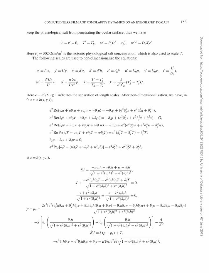
COMPUTED TEAR FILM AND OSMOLARITY DYNAMICS ON AN EYE-SHAPED DOMAIN
keep the physiological salt from penetrating the ocular surface; thus we have
u′ = v′ = 0, T ′ = T ′B, w′ = P′
c(c′ − c′
0), w′c′ = Dc∂′zc
′.
Here c′0 = 302 Osm/m3 is the isotonic physiological salt concentration, which is also used to scale c′.
The following scales are used to non-dimensionalize the equations:
x′ = L′x, y′ = L′y, z′ = d ′z, h′ = d ′h, c′ = c′0c̄, u′ = U0u, v′ = U0v, t′ = L′
U0t,
w′ = d ′U0
L′ w, p′ = μU0
L′ε2p, T = T ′ − T ′
s
T ′B − T ′
s
, J ′ = k
d ′Lm(T ′
B − T ′s)J .
Here ε = d ′/L′ 1 indicates the separation of length scales. After non-dimensionalization, we have, in0 < z < h(x, y, t),
ε2 Re(∂tu + u∂xu + v∂yu + w∂zu) = −∂xp + (ε2∂2x u + ε2∂2
y u + ∂2z u),
ε2 Re(∂tv + u∂xv + v∂yv + w∂zv) = −∂yp + (ε2∂2x v + ε2∂2
y v + ∂2z v) − G,
ε4 Re(∂tw + u∂xw + v∂yw + w∂zw) = −∂zp + ε2(ε2∂2x w + ε2∂2
y w + ∂2z w),
ε2 Re Pr(∂tT + u∂xT + v∂yT + w∂zT) = ε2(∂2x T + ∂2
y T) + ∂2z T ,
∂xu + ∂yv + ∂zw = 0,
ε2 Pec[∂t c̄ + (u∂xc̄ + v∂yc̄ + w∂zc̄)] = ε2∂2x c̄ + ε2∂2
y c̄ + ∂2z c̄,
at z = h(x, y, t),
EJ = −u∂xh − v∂yh + w − ∂th√1 + ε2(∂xh)2 + ε2(∂yh)2
,
J + −ε2∂xh∂xT − ε2∂yh∂yT + ∂zT√1 + ε2(∂xh)2 + ε2(∂yh)2
= 0,
v + ε2w∂yh√1 + ε2(∂yh)2
= u + ε2w∂xh√1 + ε2(∂xh)2
= 0,
p − pv − 2ε2[ε2(∂2x h∂xu + ∂2
y h∂yv + ∂xh∂yh(∂yu + ∂xv) − ∂xh∂xw − ∂yh∂yw) + ∂zw − ∂xh∂zu − ∂yh∂zv]√1 + ε2(∂xh)2 + ε2(∂yh)2
= −S
[∂x
(∂xh√
1 + ε2(∂xh)2 + ε2(∂yh)2
)+ ∂y
(∂yh√
1 + ε2(∂xh)2 + ε2(∂yh)2
)]− A
h3,
K̄J = δ (p − pv) + T ,
−ε2∂xh∂xc̄ − ε2∂yh∂yc̄ + ∂zc̄ = E Pecε2c̄J√
1 + ε2(∂xh)2 + ε2(∂yh)2,
153
Dow
nloaded from https://academ
ic.oup.com/im
amm
b/article-abstract/33/2/123/2875345 by University of D
elaware Library user on 07 June 2019
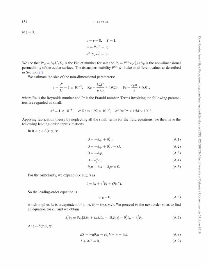
L. LI ET AL.
at z = 0,
u = v = 0, T = 1,
w = Pc(c̄ − 1),
ε2 Pecwc̄ = ∂zc̄.
We see that Pec = U0L′/Dc is the Pèclet number for salt and Pc = Ptissvwc′0/εU0 is the non-dimensional
permeability of the ocular surface. The tissue permeability Ptiss will take on different values as describedin Section 2.2.
We estimate the size of the non-dimensional parameters:
ε = d ′
L′ = 1 × 10⁻³, Re = U0L′
μ/ρ≈ 19.23, Pr = cpμ
k≈ 8.01,
where Re is the Reynolds number and Pr is the Prandtl number. Terms involving the following parame-ters are regarded as small:
ε2 = 1 × 10⁻⁶, ε2 Re ≈ 1.92 × 10⁻⁵, ε2 Re Pr ≈ 1.54 × 10⁻⁴.
Applying lubrication theory by neglecting all the small terms for the fluid equations, we then have thefollowing leading-order approximations.
In 0 < z < h(x, y, t):
0 = −∂xp + ∂2z u, (A.1)
0 = −∂yp + ∂2z v − G, (A.2)
0 = −∂zp, (A.3)
0 = ∂2z T , (A.4)
∂xu + ∂yv + ∂zw = 0. (A.5)
For the osmolarity, we expand c̄(x, y, z, t) as
c̄ = c̄0 + ε2c̄1 + O(ε4).
So the leading-order equation is∂zc̄0 = 0, (A.6)
which implies c̄0 is independent of z, i.e. c̄0 = c̄0(x, y, t). We proceed to the next order so as to findan equation for c̄0, and we obtain
∂2z c̄1 = Pec[∂t c̄0 + (u∂xc̄0 + v∂yc̄0)] − ∂2
x c̄0 − ∂2y c̄0. (A.7)
At z = h(x, y, t):
EJ = −u∂xh − v∂yh + w − ∂th, (A.8)
J + ∂zT = 0, (A.9)
154
Dow
nloaded from https://academ
ic.oup.com/im
amm
b/article-abstract/33/2/123/2875345 by University of D
elaware Library user on 07 June 2019
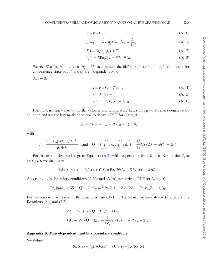
COMPUTED TEAR FILM AND OSMOLARITY DYNAMICS ON AN EYE-SHAPED DOMAIN
u = v = 0, (A.10)
p − pv = −S(∂2x h + ∂2
y h) − A
h3, (A.11)
K̄J = δ(p − pv) + T , (A.12)
∂zc̄1 = EPecc̄0J + ∇h · ∇ c̄0. (A.13)
We use ∇ = (∂x, ∂y) and Δ = (∂2x + ∂2
y ) to represent the differential operators applied on them forconvenience since both h and c̄0 are independent on z.
At z = 0:
u = v = 0, T = 1, (A.14)
w = Pc(c̄0 − 1), (A.15)
∂zc̄1 = PecPc(c̄0 − 1)c̄0. (A.16)
For the tear film, we solve for the velocity and temperature fields, integrate the mass conservationequation and use the kinematic condition to derive a PDE for h(x, y, t):
∂th + EJ + ∇ · Q − Pc(c̄0 − 1) = 0,
with
J = 1 − δ(SΔh + Ah−3)
K̄ + hand Q =
(∫ h
0u dz,
∫ h
0v dz
)= h3
12∇(SΔh + Ah−3 − Gy).
For the osmolarity, we integrate Equation (A.7) with respect to z from 0 to h. Noting that c̄0 =c̄0(x, y, t), we then have
∂zc̄1(x, y, h, t) − ∂zc̄1(x, y, 0, t) = Pec[h∂t c̄0 + ∇ c̄0 · Q] − hΔc̄0.
According to the boundary conditions (A.13) and (A.16), we derive a PDE for c̄0(x, y, t):
Pec[h∂t c̄0 + ∇ c̄0 · Q] − hΔc̄0 = E Pecc̄0J + ∇h · ∇ c̄0 − PecPc(c̄0 − 1)c̄0.
For convenience, we use c in the equations instead of c̄0. Therefore, we have derived the governingEquations (2.1) and (2.2):
∂th + EJ + ∇ · Q − Pc(c − 1) = 0,
h∂tc + ∇c · Q = EcJ + 1
Pec∇ · (h∇c) − Pc(c − 1)c.
Appendix B. Time-dependent fluid flux boundary condition
We define
Qlg(s, t) = flg(t)Q̂ls(s), Qp(s, t) = fp(t)Q̂p(s)
155
Dow
nloaded from https://academ
ic.oup.com/im
amm
b/article-abstract/33/2/123/2875345 by University of D
elaware Library user on 07 June 2019

L. LI ET AL.
in the time-dependent fluid flux BC (2.5). The formulations of flg(t), fp(t), Q̂lg(s) and Q̂p(s) are listedbelow:
flg(t) =
⎧⎪⎪⎪⎪⎪⎪⎪⎪⎪⎪⎨⎪⎪⎪⎪⎪⎪⎪⎪⎪⎪⎩
1
2
[cos
(π
2
t − tlg,on
Δtlg− π
2
)+ 1
]if |t − tlg,on| � Δtlg;
1 if tlg,on + Δtlg � t � tlg,off − Δtlg;
1
2
[cos
(π
2
t − tlg,off
Δtlg+ π
2
)+ 1
]if |t − tlg,off| � Δtlg;
0 otherwise.
(B.1)
fp(t) =
⎧⎪⎪⎪⎪⎪⎪⎪⎪⎪⎪⎨⎪⎪⎪⎪⎪⎪⎪⎪⎪⎪⎩
1
2
[cos
(π
2
t − tp,on
Δtp− π
2
)+ 1
]if |t − tp,on| � Δtp;
1 if tp,on + Δtp � t � tp,off − Δtp;
1
2
[cos
(π
2
t − tp,off
Δtp+ π
2
)+ 1
]if |t − tp,off| � Δtp;
0 otherwise.
(B.2)
Q̂lg(s) =
⎧⎪⎪⎪⎪⎪⎪⎪⎪⎪⎪⎪⎪⎪⎨⎪⎪⎪⎪⎪⎪⎪⎪⎪⎪⎪⎪⎪⎩
0 if s < slg,on − Δslg;
−1
2Q̂0lg
[cos
(π
2
s − slg,on
Δslg− π
2
)+ 1
]if |s − slg,on| � Δslg;
−Q̂0lg if slg,on + Δslg � s � slg,off − Δslg;
−1
2Q̂0lg
[cos
(π
2
s − slg,off
Δslg+ π
2
)+ 1
]if |s − slg,off| � Δslg;
0 otherwise.
(B.3)
Q̂p(s) =
⎧⎪⎪⎪⎪⎪⎪⎪⎪⎪⎪⎪⎪⎪⎪⎨⎪⎪⎪⎪⎪⎪⎪⎪⎪⎪⎪⎪⎪⎪⎩
0 if s < sp,lo − Δsp;
− Q̂0p
2(1 − pout)
[cos
(π
s − sp,lo
Δsp− π
)− 1
]if |s − sp,lo| � Δsp;
0 if sp,lo + Δsp � s � sp,up − Δsp;
− Q̂0p
2(pout)
[cos
(π
s − sp,up
Δsp− π
)− 1
]if |s − sp,up| � Δsp;
0 otherwise.
(B.4)
Parameters in the formulations are tabulated in Table B.1.
156
Dow
nloaded from https://academ
ic.oup.com/im
amm
b/article-abstract/33/2/123/2875345 by University of D
elaware Library user on 07 June 2019
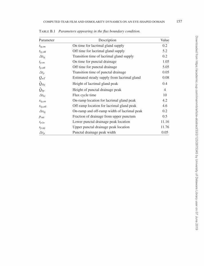
COMPUTED TEAR FILM AND OSMOLARITY DYNAMICS ON AN EYE-SHAPED DOMAIN
Table B.1 Parameters appearing in the flux boundary condition.
Parameter Description Value
tlg,on On time for lacrimal gland supply 0.2
tlg,off Off time for lacrimal gland supply 5.2
Δtlg Transition time of lacrimal gland supply 0.2
tp,on On time for punctal drainage 1.05
tp,off Off time for punctal drainage 5.05
Δtp Transition time of punctal drainage 0.05
QmT Estimated steady supply from lacrimal gland 0.08
Q̂0lg Height of lacrimal gland peak 0.4
Q̂0p Height of punctal drainage peak 4
Δtbc Flux cycle time 10
slg,on On-ramp location for lacrimal gland peak 4.2
slg,off Off-ramp location for lacrimal gland peak 4.6
Δslg On-ramp and off-ramp width of lacrimal peak 0.2
pout Fraction of drainage from upper punctum 0.5
sp,lo Lower punctal drainage peak location 11.16
sp,up Upper punctal drainage peak location 11.76
Δsp Punctal drainage peak width 0.05
157
Dow
nloaded from https://academ
ic.oup.com/im
amm
b/article-abstract/33/2/123/2875345 by University of D
elaware Library user on 07 June 2019


![Membrane-bound mucins and mucin terminal glycans ... · associated with higher morbidity and mortality[1-7]. Mucins, heavily glycosylated high-molecular-weight glycoproteins, are](https://static.fdocuments.net/doc/165x107/5fcbfea3277df0670a5fee63/membrane-bound-mucins-and-mucin-terminal-glycans-associated-with-higher-morbidity.jpg)
