Computationally Efficient Forecasting Procedures for Kuhn-Tucker Consumer Demand

Model Systems: Application to Residential Energy Consumption Analysis

Abdul Rawoof Pinjari (Corresponding Author) University of South Florida Department of Civil & Environmental Engineering 4202 E. Fowler Ave., Tampa, FL 33620 Tel: 813-974- 9671, Fax: 813-974-2957 E-mail: apinjari@usf.edu

Chandra Bhat The University of Texas at Austin Dept of Civil, Architectural & Environmental Engineering 1 University Station C1761, Austin, TX 78712-0278 Tel: 512-471-4535, Fax: 512-475-8744 E-mail: bhat@mail.utexas.edu

ABSTRACT

This paper proposes simple and computationally efficient forecasting algorithms for a Kuhn-Tucker (KT) consumer demand model system called the Multiple Discrete-Continuous Extreme Value (MDCEV) model. The algorithms build on simple, yet insightful, analytical explorations with the Kuhn-Tucker conditions of optimality that shed new light on the properties of the model. Although developed for the MDCEV model, the proposed algorithm can be easily modified to be used for other KT demand model systems in the literature with additively separable utility functions. The MDCEV model and the forecasting algorithms proposed in this paper are applied to a household-level energy consumption dataset to analyze residential energy consumption patterns in the United States. Further, simulation experiments are undertaken to assess the computational performance of the proposed (and existing) KT demand forecasting algorithms for a range of choice situations with small and large choice sets.

Keywords: Discrete-continuous models, Kuhn-Tucker consumer demand systems, MDCEV

model, forecasting procedure, residential energy consumption, climate change impacts, welfare

analysis

1

1. INTRODUCTION

In several consumer demand situations, consumer behavior may be associated with the choice of multiple alternatives simultaneously, along with a continuous choice component of “how much to consume” for the chosen alternatives. Such multiple discrete-continuous choice situations are being increasingly recognized and modeled in the recent literature in transportation, marketing, and economics.

A variety of modeling frameworks have been used to analyze multiple discrete-continuous choice situations. These can be broadly classified into: (1) statistically stitched multivariate single discrete-continuous models (see, for example, Srinivasan and Bhat, 2006), and (2) utility maximization-based Kuhn-Tucker (KT) demand systems (Hanemann, 1978; Wales and Woodland, 1983; Kim et al., 2002; Phaneuf et al., 2000; von Haefen and Phaneuf, 2005; Bhat, 2005 and 2008). Between the two approaches, the KT demand systems are more theoretically grounded in that they employ a unified utility maximization framework for simultaneously analyzing the multiple discrete and continuous choices. Further, these model systems accommodate fundamental features of consumer behavior such as satiation effects through diminishing marginal utility with increasing consumption.

The KT demand systems have been known for quite some time, dating back at least to the research works of Hanemann (1978) and Wales and Woodland (1983). However, it is only in the past decade that practical formulations of the KT demand system have appeared in the literature. Recent applications include, but are not limited to, individual activity participation and time-use studies (Bhat, 2005; Habib and Miller, 2009; Pinjari et al., 2009, Rajagopalan et al. 2009; Pinjari and Bhat 2010), household travel expenditure analyses (Rajagopalan and Srinivasan, 2008; Ferdous et al., 2010), household vehicle ownership and usage forecasting (Ahn et al., 2007; Fang, 2008; and Bhat et al., 2008), outdoor recreational demand studies (Phaneuf et al., 2000; von Haefen et al., 2004; and von Haefen and Phaneuf, 2005), and grocery purchase analyses (Kim et al., 2002). As indicated by Vasqez-Lavín and Hanemann (2009), this surge in interest may be attributed to the strong theoretical basis of KT demand systems combined with recent developments in simulation techniques.

Within the KT demand systems, the recently formulated multiple discrete-continuous extreme value (MDCEV) model structure by Bhat (2005, 2008) is particularly attractive due to its closed form, its intuitive and clear interpretation of the utility function parameters, and its generalization of the single discrete multinomial logit choice probability structure. In recent papers, the basic MDCEV framework has been expanded in several directions, including the incorporation of more general error structures to allow flexible inter-alternative substitution patterns (Pinjari and Bhat, 2010; Pinjari, 2011).

Despite the many developments and applications, a simple and very quick forecasting procedure has not been available for the MDCEV and other KT demand model systems. On the other hand, since the end-goal of most model development and estimation is forecasting, policy evaluation, and/or welfare analysis, development of a simple and easily applicable forecasting procedure is a critical issue in the application of KT demand model systems. Currently available forecasting methods are either enumerative or iterative in nature, are not very accurate, and require long computation times.

2

In this paper, we propose computationally efficient forecasting algorithms for the MDCEV model.1 The algorithms build on simple, yet insightful, analytic explorations with the KT conditions that shed new light on the properties of the MDCEV model. For specific utility functional forms used in many MDCEV model applications, the proposed approach is non-iterative in nature, and results in analytically expressible consumption quantities. Even with more general utility forms that fall within the class of additively separable utility functions, we are able to employ the properties of the MDCEV model presented in this paper to design efficient (albeit iterative) forecasting algorithms. In addition, we formulate variants to the proposed algorithms that remain computationally efficient even in situations with large choice sets. Further, the insights gained from the analysis of the KT conditions also enable us to develop efficient forecasting procedures for other non-MDCEV KT demand systems with additively separable utility functions.

As a demonstration of the effectiveness of the proposed algorithms, we present an application to analyze residential energy consumption patterns in the U.S., using household-level energy consumption data from the 2005 Residential Energy Consumption Survey (RECS) conducted by the Energy Information Administration (EIA). This application provides insights into the influence of household, house-related, and climatic factors on households’ consumption patterns of different types of energy, including electricity, natural gas, fuel oil, and liquefied petroleum gas (LPG). Prediction exercises with the proposed algorithms and currently used algorithms highlight the significant computational efficiency of the proposed algorithms. In addition, we present simulation experiments to assess the computational performance of the proposed algorithms vis-à-vis existing algorithms in situations with large choice sets.

The remainder of the paper is organized as follows. The next section presents the challenge associated with forecasting with the MDCEV model, and describes currently used forecasting procedures in the literature. Section 3 highlights some new properties of the MDCEV model. Building on these properties, Section 4 presents new forecasting algorithms tailored for different types of utility specifications under different choice situations, ranging from very small to very large choice sets. In addition, a discussion is provided on how similar forecasting algorithms can be developed for other KT demand system models. Section 5 presents an application of the MDCEV model to analyze residential energy consumption patterns in the U.S., using the 2005 RECS data. Section 6 presents several prediction experiments with the RECS data as well as other, simulated data to assess the computational performance of the proposed forecasting algorithms vis-à-vis existing approaches. In addition, this section includes hypothetical policy simulations to predict the impact of different climate change-related scenarios on residential energy consumption patterns. Section 7 summarizes and concludes the paper.

2 FORECASTING WITH KT DEMAND MODEL SYSTEMS The MDCEV and other KT demand modeling systems are based on a resource allocation formulation. Specifically, it is assumed that consumers operate with a finite amount of available resources (i.e., a budget), such as time or money. Their decision-making mechanism is assumed to be driven by an allocation of the limited amount of resources to consume various goods/alternatives to maximize the utility derived from consumption. Further, a stochastic utility

1 From now on, and throughout the paper, we use the term efficient interchangeably with the term computationally efficient (i.e., computationally fast). The reader should not confuse this with statistical/econometric efficiency.

3

framework is used to recognize the analyst’s lack of awareness of factors affecting consumer decisions. In addition, a non-linear utility function is employed to incorporate important features of consumer behavior, including: (1) the diminishing nature of marginal utility with increasing consumption (i.e., satiation effects), and (2) the possibility of consuming multiple goods as opposed to a single good. To summarize, the KT demand modeling frameworks are based on a stochastic (due to the stochastic utility framework), constrained (due to the budget constraint), non-linear (due to satiation effects) utility optimization formulation.

In most KT demand system models, the stochastic KT first order conditions of optimality form the basis for model estimation. Specifically, an assumption that stochasticity (or unobserved heterogeneity) is generalized extreme value (GEV) distributed leads to closed form consumption probability expressions (Bhat 2005 and 2008; Pinjari 2011; von Haefen et al., 2004), facilitating a straightforward maximum likelihood estimation of the model parameters. Once the model parameters are estimated, forecasting or policy analysis exercises involve solving the stochastic, constrained, non-linear utility maximization problem for the optimal consumption quantities of each decision-maker. Unfortunately, there is no straightforward analytic solution to this problem. The typical approach is to adopt a constrained non-linear optimization procedure at each of several simulated values drawn from the distribution of unobserved heterogeneity. This constrained non-linear optimization procedure itself is based on either an enumeration technique or an iterative technique. The enumerative technique (used by Phaneuf et al., 2000) involves enumeration of all possible sets of alternatives that the decision-maker can potentially choose to consume. Specifically, if there are K available choice alternatives, assuming not more than one essential Hicksian composite good (or outside good)2, one can enumerate 2K-1 possible choice set solutions to the consumer’s utility maximization problem. Clearly, such a brute-force method becomes computationally burdensome and impractical even with a modest number of available choice alternatives/goods. Thus, for medium to large numbers of choice alternatives, an iterative optimization technique has to be used. As with any iterative technique, optimization begins with an initial solution (for consumptions) that is then improved in subsequent steps (or iterations) by moving along specific directions using the gradients of the utility functions, until a desired level of accuracy is reached. Most studies in the literature use off-the-shelf optimization programs (such as the constrained maximum likelihood library of GAUSS) to undertake such iterative optimization. However, the authors’ experience with iterative methods of forecasting in prior research efforts indicates several problems, including long computation times and convergence issues.

More recently, von Haefen et al. (2004) proposed another iterative forecasting algorithm designed based on the insight that the optimal consumptions of all goods can be derived if the optimal consumption of the outside good is known. Specifically, conditional on the simulated values of unobserved heterogeneity, von Haefen et al. begin their iterations by setting the lower bound for the consumption of the outside good to zero and the upper bound to be equal to the budget. The average of the lower and upper bounds is used to obtain the initial estimate of the outside good consumption. Based on this, the amounts of consumption of all other inside goods are computed using the KT conditions. Next, a new estimate of consumption of the outside good is obtained by subtracting the budget on the consumption of the inside goods from the total budget available. If this new estimate of the outside good is larger (smaller) than the earlier

2 Several KT demand system models generally include an essential Hicksian good (or outside good, or numeraire good), which is always consumed by the decision-makers.

4

estimate, the earlier estimate becomes the new lower (upper) bound of consumption for the outside good, and the iterations continue until the difference between the lower and upper bounds is within an arbitrarily designated threshold. This numerical bisection iterative process relies on the strict concavity of the utility function. Further, to circumvent the need to perform predictions over the entire distribution of unobserved heterogeneity, von Haefen et al. condition on the observed choices.3 Based on “Monte Carlo experiments with low-dimensional choice sets”, they indicate that, relative to the unconditional approach (of simulating the entire distribution of unobserved heterogeneity), the conditional approach requires about 1/3rd the simulations (of conditional unobserved heterogeneity) and time to produce stable estimates of mean consumptions and welfare measures. Overall, this combination of the numerical bisection algorithm with the conditional approach is clever and clearly more efficient than using a generic optimization procedure with the unconditional approach. However, the numerical bisection algorithm is still iterative and can involve a substantial amount of time. At the same time, in many situations, the estimated model needs to be applied to data outside the estimation sample, in which case the conditional approach cannot be used. For instance, in the travel demand field, models are estimated with an express intent to apply them for predicting the activity-travel patterns in the external (to estimation sample) data representing the study area population. This implies that the iterative numerical bisection algorithm has to be applied using the unconditional approach, which could further increase computation time. The point is that there is a computational benefit to using a non-iterative optimization procedure rather than an iterative procedure, which can then be used with the conditional approach when possible or with the unconditional approach if needed. Further, and more importantly, the von Haefen et al algorithm is applicable only in the case with the presence of an outside good. To be more precise, their approach can be applied only if the analyst knows apriori at least one good chosen by the consumer. In situations with an outside good, it is already known that the outside good is one of the consumed alternatives. However, in situations with no outside good, their approach doesn’t provide any lead to the analyst on which alternative is consumed (or not consumed), a critical prerequisite for obtaining the consumption forecasts.

3 THE MDCEV MODEL: STRUCTURE AND PROPERTIES

This section draws from Bhat (2008) to briefly discuss the structure of the MDCEV model (Section 3.1) and derives some fundamental properties of the model (Section 3.2) that will form the basis for formulating the forecasting algorithm.

3.1 Model Structure

Consider the following additively separable utility function as in Bhat (2008):

1

1 1

21

1( ) 1 1 ; 0, 0 1, 0

kKk k

k k k k

k k k

tU t

α

α γψ ψ ψ α γ

α α γ=

= + + − > ≤ ≤ >

∑t (1)

3 To do so, they simulate the unobserved heterogeneity that corresponds to the observed choices in the data (that is, they simulate the elements of the error vector for each individual so as to exactly replicate the observed consumptions of the individual in the estimation sample). Using these simulated values of conditional (on observed choices) unobserved heterogeneity, they apply the numerical bisection algorithm to perform predictions for the policy case and subsequently compute the welfare change from the base case to policy case. See von Haefen (2003) for a discussion on the advantages of incorporating observed choices into policy analyses.

5

In the above expression, U(t) is the total utility accrued from consuming t (a Kx1 vector with

non-negative consumption quantities kt ; k = 1,2,…,K) amount of the K alternatives available to

the decision maker. The kψ terms (k = 1,2,…,K), labeled as baseline utility parameters, represent

the marginal utility of one unit of consumption of alternative k at the point of zero consumption

for that alternative. Through the kψ terms, the impact of observed and unobserved alternative

attributes, decision-maker attributes, and the choice environment attributes may be introduced as

exp( )k k kzψ β ε′= + , where kz contains the observed attributes and kε is a random disturbance

capturing the unobserved factors. The kα terms (k = 1,2,…,K), labeled as satiation parameters

(0 1)kα< ≤ , capture satiation effects by reducing the marginal utility accrued from each unit of

additional consumption of alternative k.4 The kγ terms (k = 2,3,…,K), labeled as translation

parameters, play a similar role of satiation as that of kα terms, and an additional role of

translating the indifference curves associated with the utility function to allow corner solutions (i.e., accommodate the possibility that decision-makers may not consume all alternatives). As it

can be observed, there is no kγ term for the first alternative for it is assumed to be an essential

Hicksian composite good (or outside good or essential good) that is always consumed (hence there is no need for a corner solution). Finally, the consumption-based utility function in (1) can

be expressed in terms of expenditures ( ke ) and prices ( kp ) as:5

1

11

21 1

1( ) 1 1 ,

kKk k

k

k k k k

eeU

p p

ααγ

ψ ψα α γ=

= + + −

∑e where k

k

k

ex

p= (2)

From the analyst’s perspective, decision-makers maximize the random utility given by Equation

(2) subject to a linear budget constraint and non-negativity constraints on ke :

1

(where is the total budget) and 0 ( 1,2,..., )K

k k

k

e E E e k k K=

= ≥ ∀ =∑ (3)

The optimal consumptions (or expenditure allocations) can be found by forming the Lagrangian and applying the Kuhn-Tucker (KT) conditions. The Lagrangian function for the problem is:

L

1

11

2 11 1

11 1

kK Kk k

k k

k kk k k

eee E

p p

ααγ

ψ ψ λα α γ= =

= + + − − −

∑ ∑ ,

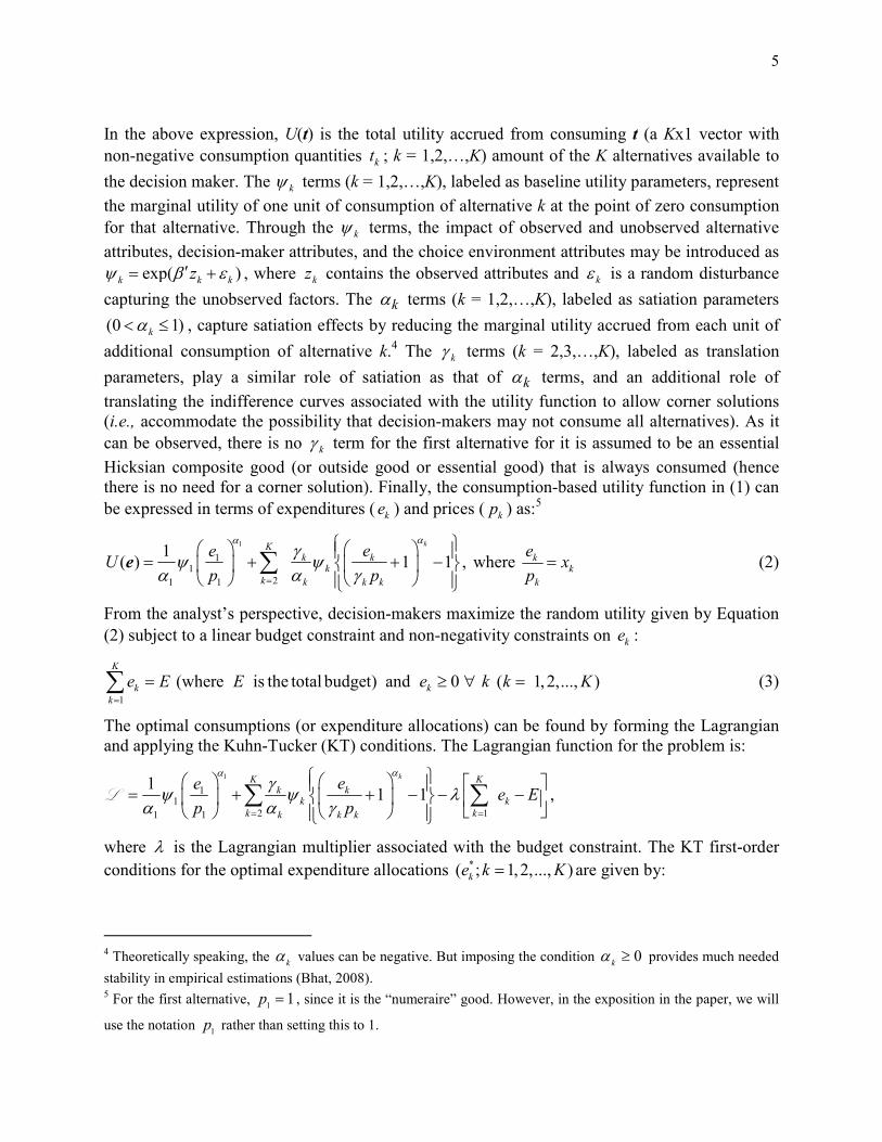
where λ is the Lagrangian multiplier associated with the budget constraint. The KT first-order conditions for the optimal expenditure allocations *( ; 1,2,..., )ke k K= are given by:

4 Theoretically speaking, the k

α values can be negative. But imposing the condition 0k

α ≥ provides much needed

stability in empirical estimations (Bhat, 2008). 5 For the first alternative,

11p = , since it is the “numeraire” good. However, in the exposition in the paper, we will

use the notation 1p rather than setting this to 1.

6

1 1*

1 1

1 1

0e

p p

αψ

λ−

− =

, since *

1 0e > ,

1*

1 0

k

k k

k k k

e

p p

αψ

λγ

−

+ − =

, if * 0,ke > (k = 2,…, K) (4)

1*

1 0

k

k k

k k k

e

p p

αψ

λγ

−

+ − <

, if * 0,ke = (k = 2,…, K)

As indicated earlier, these stochastic KT conditions form the basis for model estimation.

Specifically, an assumption that the kε terms (i.e., the stochastic components of the kψ terms)

are independent and identically distributed type-I extreme value (or Gumbel) distributed leads to closed form consumption probability expressions that can be used to form the likelihoods for maximum likelihood estimation (see Bhat, 2005). Next, using these same stochastic KT conditions, we derive a few properties of the MDCEV model that can be exploited to develop a highly efficient forecasting algorithm.

3.2 Model Properties

Property 1: The price-normalized baseline utility of a chosen good is always greater than that of

a good that is not chosen.

ji

i jp p

ψψ >

if ‘i’ is a chosen good and ‘j’ is not a chosen good. (5)

Proof: The KT conditions in (4) can be rewritten as:

1 1*

1 1

1 1

e

p p

αψ

λ−

=

,

1*

1

k

k k

k k k

e

p p

αψ

λγ

−

+ =

, if * 0,ke > (k = 2,…, K) (i.e., for all chosen goods) (6)

k

kp

ψλ< , if * 0,ke = (k = 2,…, K) (i.e., for all goods that are not chosen)

The above KT conditions can further be rewritten as:

7

1

1

1 1* *

*1 1

1 1

1*

*1 1

1 1

1 , if 0, ( 2,3,..., )

< , if 0, ( 2,3,..., )

k

k kk

k k k

kk

k

e ee k K

p p p p

ee k K

p p p

α α

α

ψ ψγ

ψ ψ

− −

−

= + > =

= =

(7)

Now, consider two alternatives ‘i’ and ‘j’, of which ‘i’ is chosen and ‘j’ is not chosen by a consumer. For that consumer, the above KT conditions for alternatives ‘i’ and ‘j’ can be written as:

1

1

1 1* *

1 1

1 1

1*

1 1

1 1

1 , and

<

i

i i

i i i

j

j

e e

p p p p

e

p p p

α α

α

ψ ψγ

ψ ψ

− −

−

= +

(8)

Further, since

1*

1

j

j

j j

e

p

α

γ

−

+

is always greater than 1, one can write the following inequality:

1 111 1** *

1 1 1 1

1 1 1 1

< 1

i

j i

j i i

ee e

p p p p p p

αα αψ ψ ψ

γ

−− − < +

(9)

As one can observe, the third term in the above inequality is nothing but i

ip

ψ

, and the second

term is λ . Thus, one can rewrite the inequality in (9) as:

< j i

j ip p

ψ ψλ

<

(10)

Now, by the transitive property of inequality of real numbers, the above inequality implies a

fundamental property of the MDCEV model that ji

i jp p

ψψ >

. In words, the price-normalized

baseline utility of a chosen good is always greater than that of a good that is not chosen.

Corollary 1.1: It naturally follows from the property above that when all the K

alternatives/goods available to a consumer are arranged in a descending order of their price-

normalized baseline utility values (with the outside good being the first in the order), and if it is

8

known that the number of chosen alternatives is M, then one can easily identify the chosen

alternatives as the first M alternatives in the arrangement.6

Corollary 1.2: Another important observation to be made from Equation (10) is that the Lagrange multiplier of the consumer’s utility maximization problem (i.e., the marginal utility at

optimal consumption) is always greater than the price-normalized utility of any not-chosen good,

but less than that of any chosen good. It naturally follows from this property that λ is greater than the highest price-normalized baseline utility among the not-chosen goods, but less than the

lowest price-normalized baseline utility among the chosen goods.

Property 2: The minimum consumption amount of the outside good is

1

1

11

1

(2,3,..., )

.

max k

k Kk

p

p

αψ

ψ

−

∀ =

Proof: Use the first and third KT conditions in (6), and consider market baskets that involve only

the consumption of the outside good (i.e., * 0, 1)ke k= ∀ > . At these market baskets, one can write

the following:

1 1*

1 1

1 1

; (2,3,..., ),k

k

ek K

p p p

αψ ψ

−

< ∀ =

or,

1 1*

1 1

(2,3,..., )1 1

max .k

k Kk

e

p p p

αψ ψ

−

∀ =

<

Hence,

1

1

11

*11

1

(2,3,..., )

.

max k

k Kk

pe

p

p

αψ

ψ

−

∀ =

>

(11)

In words, the right side of the above equation represents the “minimum” amount of consumption of the outside good. The interpretation is that, after the “minimum” amount of the outside good is consumed, all other goods (and the outside good) start competing for the remaining amount of the budget. Thus, if the budget amount is less than that corresponding to the minimum consumption of the outside good given in (11), no other good will be consumed. Note also that if there is no price variation across the consumption alternatives, the distribution of the minimum consumption of the outside good can be derived as a log-logistic variable (given that

exp( )k k kzψ β ε′= + ).

6 Note that the converse of this property may not always hold true. That is, given the price-normalized utilities of two alternatives, one cannot say with certainty if one or both of the alternatives are chosen.

9

Property 3: When all the satiation parameters ( )kα are equal, and if the corner solutions (or

discrete choices) are known (i.e., if the chosen and non-chosen alternatives are known), the

Lagrange multiplier of the utility maximization as well as the continuous optimal consumption

choices of the chosen goods can be expressed in an analytic form.

Proof 7: Using the first and second KT conditions in (6), and assuming without loss of generality

that the first M goods are chosen, one can express the optimal consumptions as:

1

1* 11 1

1 1

, ande p

p

α

λψ

− =

(12) 1

* 1

1 ; (2,3,..., )k

k kk

k k

e pk M

p

α

λ γψ

−

= − ∀ =

8

Using these expressions, the budget constraint in (3) can be written as:

1

11

111

1

21

1k

Mk

k k

k k

ppp p E

αα

λ λ γψ ψ

−−

=

+ − =

∑ 9 (13)

From the above equation, and assuming that all satiation ( )kα parameters as equal to α , the Lagrange multiplierλ can be expressed analytically as:

1

2

11

111

1

21

M

k k

k

Mk

k k

k k

E p

p pp p

α

αα

γλ

ψψγ

−

=

−−

=

+ = +

∑

∑

(14)

The above expression for λ can be substituted back into the expressions in (12) to obtain the following analytic expressions for optimal consumptions:

7 This is a known property of KT demand model systems. But we provide the proof here for completeness.

8 Although this expression involves a subtraction, it is not possible to obtain negative predictions. One can verify

this by applying the KT condition inequality: ( / )k kp kλ ψ> ∀ ∈{chosen alternatives} to see that the second expression always provides positive predictions. 9 The expression on the left side of this budget constraint equation is a monotonically decreasing function of λ . This property will be useful later.

10

1

11

*211

11

1 111

1

21

M

k k

k

Mk

k k

k k

E ppe

p

p pp p

α

αα

ψγ

ψψγ

−

=

−−

=

+

=

+

∑

∑

(15)

1

1

*2

11

111

1

21

1 ; (2,3,..., )

Mk

k k

kkkk

Mkk

k k

k k

E ppe

k Mp

p pp p

α

αα

ψγ

γψψ

γ

−

=

−−

=

+ = − ∀ =

+

∑

∑

. (16)

The reader will note here that the expressions in Equations (14), (15) and (16) contain terms corresponding to the consumed (i.e. chosen) goods only.

4 EFFICIENT FORECASTING ALGORITHMS FOR MDCEV AND OTHER KT

DEMAND MODELS

In this section, using the properties discussed in the preceding section, we propose efficient forecasting algorithms for MDCEV model and other KT demand systems. Section 4.1 presents a non-iterative forecasting algorithm for the MDCEV model with the following utility function:

11 1

21

1( ) exp( ) exp( ) 1 1 ,

Kk k

k k

k k k

eeU z z

p p

ααγ

β ε β εα α γ=

′ ′= + + + + −

∑e (17)

As indicated in Bhat (2008), this is a -profileγ utility function in that the kγ parameters are

different across the choice alternatives but the satiation ( kα ) parameters are constrained to be

equal (to α ) across all choice alternatives. Section 4.2 presents a similar (but iterative) algorithm for more general utility functions that allow for different kα parameters across choice

alternatives. Section 4.3 presents variants to the proposed algorithms for situations with large choice sets. Section 4.4 discusses how such efficient forecasting algorithms can be designed for other KT demand systems in the literature with additively separable utility functions.

4.1 Forecasting Algorithm for the MDCEV model with γ -profile Utility Functions: An Incremental Enumeration Method

The proposed algorithm comprises four basic steps as outlined below. Step 0: Assume that only the outside good is chosen and let the number of chosen goods M = 1.

Step 1: Given the input data ( kz , kp ), model parameters ( β , kγ ,α ), and the simulated error term

( kε ) draws, compute the price-normalized baseline utility values ( )k kpψ for all

alternatives. Arrange all the K alternatives available to the consumer in the descending order of their price-normalized baseline utility values (with the outside good in the first place). Go to step 2.

Step 2: Compute the value of λ using equation (14). Go to step 3.

11

Step 3: If λ > 1

1

M

Mp

ψ +

+

(i.e., the price-normalized baseline utility of alternative in position M+1),

compute the optimal consumptions of the first M alternatives in the above descending order using equations in (15) and (16). Set the consumptions of other alternatives as zero and stop.

Else, go to step 4. Step 4: M = M+1.

If (M = K), compute the optimal consumptions using equations in (15) and (16) and stop.

Else, go to step 2.

4.1.1 Application of the Algorithm

The algorithm outlined above can be applied a large number of times with different simulated

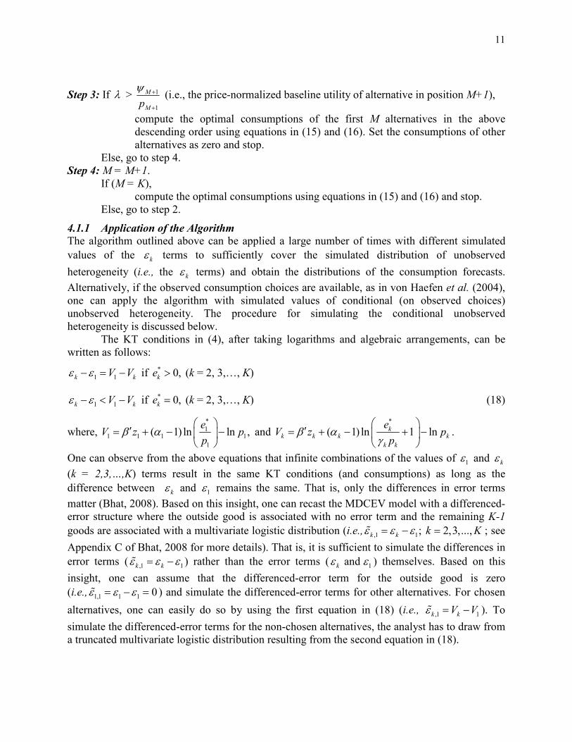
values of the kε terms to sufficiently cover the simulated distribution of unobserved heterogeneity (i.e., the kε terms) and obtain the distributions of the consumption forecasts. Alternatively, if the observed consumption choices are available, as in von Haefen et al. (2004), one can apply the algorithm with simulated values of conditional (on observed choices) unobserved heterogeneity. The procedure for simulating the conditional unobserved heterogeneity is discussed below. The KT conditions in (4), after taking logarithms and algebraic arrangements, can be written as follows:

1 1k kV Vε ε− = − if * 0,ke > (k = 2, 3,…, K)

1 1k kV Vε ε− < − if * 0,ke = (k = 2, 3,…, K) (18)

where, *

11 1 1 1

1

( 1) ln ln ,e

V z pp

β α

′= + − −

and *

( 1) ln 1 lnkk k k k

k k

eV z p

pβ α

γ

′= + − + −

.

One can observe from the above equations that infinite combinations of the values of 1ε and kε (k = 2,3,…,K) terms result in the same KT conditions (and consumptions) as long as the

difference between kε and 1ε remains the same. That is, only the differences in error terms matter (Bhat, 2008). Based on this insight, one can recast the MDCEV model with a differenced-error structure where the outside good is associated with no error term and the remaining K-1

goods are associated with a multivariate logistic distribution (i.e., ,1 1; 2,3,...,k k k Kε ε ε= − =ɶ ; see

Appendix C of Bhat, 2008 for more details). That is, it is sufficient to simulate the differences in

error terms ( ,1 1k kε ε ε= −ɶ ) rather than the error terms ( 1 and kε ε ) themselves. Based on this insight, one can assume that the differenced-error term for the outside good is zero

(i.e., 1,1 1 1 0ε ε ε= − =ɶ ) and simulate the differenced-error terms for other alternatives. For chosen

alternatives, one can easily do so by using the first equation in (18) (i.e., ,1 1k kV Vε = −ɶ ). To

simulate the differenced-error terms for the non-chosen alternatives, the analyst has to draw from a truncated multivariate logistic distribution resulting from the second equation in (18).

12

4.1.2 Intuitive Interpretation of the Algorithm

The proposed algorithm builds on the insight from corollary 1.1 that if the number of chosen alternatives is known, one can easily identify the chosen alternatives by arranging the price-normalized baseline utility values in a descending order. Subsequently, one can compute the optimal consumptions of the chosen alternatives using Equations (15) and (16). The only issue, however, is that the number of chosen alternatives is unknown apriori. To find this out, the algorithm begins with an assumption that only one alternative (i.e., the outside good) is chosen and verifies this assumption by examining the KT conditions (i.e., the condition in Step 3) for other (assumed to be) non-chosen goods. If the KT conditions (i.e., the condition in Step 3) are met, the algorithm stops. Else, at least the next alternative (in the order of the price-normalized baseline utilities) has to be among the chosen alternatives. Then, the KT conditions (i.e., the condition in step 3) are verified again by assuming that the next alternative is among the chosen alternatives. These basic steps are repeated until either the KT conditions (i.e., the condition in step 3) are met or the assumed number of chosen alternatives reaches the maximum number (K). As one may note from the above description, the KT conditions are essentially replaced

by a single condition (involving the Lagrange multiplierλ ) in Step 3 of the algorithm. This condition is equivalent to verifying if λ is greater than the highest price-normalized baseline utility among the not-chosen goods (see corollary 1.2). To understand this better, recall from the equations in (6) that verifying the KT conditions in this algorithm is equivalent to verifying the

condition k

kp

ψλ > for all goods that are assumed to have not been chosen. Obviously, verifying

the condition in Step 3 (i.e., if λ is greater than the highest price-normalized baseline utility of all goods assumed to have not been chosen) is a more efficient way of doing so.10 The proposed algorithm involves enumeration of the choice baskets in a computationally efficient fashion. In fact, the algorithm begins with identifying a single alternative (outside good) that may be chosen. If the KT conditions are not met for this choice basket, the algorithm identifies a two-alternative choice basket and so on, till the number of chosen alternatives is determined. Thus, the number of times the algorithm enumerates choice baskets is equal to the number of chosen alternatives in the optimal consumption portfolio, which is at most equal to (but many times less than) the total number of available alternatives (K). Thus we label this algorithm an “incremental enumeration algorithm” Another feature of the algorithm is that it is non-iterative in nature, which makes it highly efficient compared to other iterative approaches. 11 Further, coding the algorithm using vector and matrix notation in a matrix programming language significantly reduces the computational burden even with large number of choice alternatives and observations. Also, due to the

convenient -profileγ utility specification, the algorithm is accurate with no room for any

inaccuracy (unlike the existing iterative procedures discussed earlier), as it uses analytic expressions for the optimal consumption computations.

10 At the beginning of the algorithm, when only the outside good is assumed to be consumed, the condition in Step 3 of the algorithm is equivalent to the “minimum consumption” condition in Equation (11). 11

Strictly speaking, one may view our proposed approach as iterative in (the literal sense) that steps 2-4 in Section

4.1 are iterated until the number of chosen alternatives is determined. However, in the spirit of the term “iterative” used in general for numerically-based computationally intensive iterations, we call our approach non-iterative to emphasize that the overall algorithm is analytical (as opposed to being numerical) in nature. Further, we believe that the proposed approach classifies better as enumerative (as identified in the earlier paragraph) than iterative in nature.

13

In summary, the proposed algorithm is simple and efficient. The only limitation of this

algorithm is that it is designed to be used with the -profileγ utility specification that restricts the

kα parameters of all choice alternatives to be equal. Admittedly, the -profileγ utility

specification is not the most general form within the class of additively separable utility

functions. However, as indicated by Bhat (2008), both the kγ and kα parameters serve the role

of allowing differential satiation effects across the choice alternatives. Due to the overlapping

roles played by these parameters, attempts to estimate utility functions that allow both the kγ and

kα parameters to vary across alternatives may lead to severe empirical identification issues and

estimation breakdowns. Further, “for a given kψ value, it is possible to closely approximate a

sub-utility function based on a combination of kγ and kα values with a sub-utility function

solely based on kγ or kα values” (Bhat, 2008). For these reasons, and given the ease of

forecasting with the proposed algorithm, we suggest an estimation of the -profileγ utility

function. Nevertheless, the insights obtained from the properties discussed in the preceding section (and parts of this algorithm) can be used to design an efficient (albeit iterative) algorithm

for cases when kα parameters vary across alternatives, as discussed next.

4.2 Forecasting Algorithm for the MDCEV model with General Utility Functions:

Incremental Enumeration Combined with Bisection over the λ -Space Let λ and E be estimates of λ (the Lagrange multiplier) and E (the budget amount), respectively, and let λδ and Eδ be the tolerance values (for estimatingλ and E, respectively)

which can be as small as desired. Let ˆLλ and ˆUλ be the lower and upper bounds of λ . Based on

the budget constraint Equation (13), define E (the estimate of E) as a function of λ (estimate of λ ) as below:

1

11

111

1

21

ˆ ˆˆ 1k

Mk

k k

k k

ppE p p

αα

λ λ γψ ψ

−−

=

= + −

∑ . (19)

The proposed algorithm comprises six basic steps as outlined below.

Step 0: Assume that only the outside good is chosen and let the number of chosen goods M = 1.

Step 1: Given the input data ( kz , kp ), model parameters ( β , kγ ,α ) and the simulated error term

( kε ) draws, compute the price-normalized baseline utility values ( )exp( )k k kz pβ ε′ + for

all alternatives. Arrange all the K alternatives available to the consumer in a descending order of their price-normalized baseline utility values (with the outside good in the first place).

Step 2: Let λ = 1

1

M

Mp

ψ +

+

, the price-normalized baseline utility of the alternative in position M+1.

Substitute λ into Equation (19) to obtain an estimate E of E . Step 3: If E <E

Go to step 4.

Else, if E > E

14

1

1

and M ML U

M Mp p

ψ ψλ λ+

+

= = (because 1

1

M M

M Mp p

ψ ψλ+

+

< < )

Go to step 5 to estimate λ via numerical bisection. Step 4: M = M+1.

If M < K Go to step 2. Else, if M = K

0 and KL U

Kp

ψλ λ= = (because 0 K

Kp

ψλ< < )

Go to step 5 to estimate λ via numerical bisection. Step 5: Step 5.1: Let ˆ ( ) / 2L Uλ λ λ= + and use Equation (19) to obtain an estimate E of E .

Step 5.2: If ( )ˆL U Eor E Eλλ λ δ δ− ≤ − ≤

Go to step 6.

Else, if E E<

Update the upper bound of λ as ( ) / 2U L Uλ λ λ= + , and go to step 5.1

Else, if E E>

Update the lower bound of λ as ( ) / 2L L Uλ λ λ= + , and go to step 5.1

Step 6: Compute the optimal consumptions of the first M alternatives in the above descending order using equations in (12). Set the consumptions of other alternatives as zero and stop.

As can be observed, the above algorithm is similar to the algorithm in Section 4.1 in that the choice alternatives are arranged in a descending order by the price-normalized baseline utility values. Further, the algorithm begins with an assumption that only one alternative is chosen (i.e., M =1) and builds on the following insights:

1. The value of the Lagrange multiplier λ is greater than the highest price-normalized baseline utility among the not-chosen goods, but less than the lowest price-normalized baseline utility among the chosen goods (corollary 1.2).

2. The left side of the budget constraint Equation (13) is a monotonically decreasing function of

λ . Thus, in Equation (18), the value of E increases monotonically as the value of λ decreases (see footnote 7).

Based on these insights, as indicated in step 2, the algorithm starts with an estimate λ of λ as the price-normalized baseline utility of the alternative in the (M+1)th position in the above

descending order, and a corresponding estimate E of E . Then step 3 verifies if the estimated

amount of budget E is less than the actual amount of budget E available to the decision-maker.

If so, the number of chosen alternatives M is increased by 1 (see step 4) and the value of λ is updated to the price-normalized baseline utility of the next alternative in the arrangement (see

step 2). This process is repeated until either E exceeds E (step 3), or M = K (step 4). At this point, the chosen alternatives are known (as the first M alternatives in the descending order of price-normalized utility values). Further, an upper bound (lowest price-normalized baseline utility among the chosen alternatives) and a lower bound (highest price-normalized baseline

utility among the not-chosen alternatives, or zero) are also obtained forλ . Given these bounds forλ , and the property that E decreases monotonically with λ , step 5 follows a simple

15

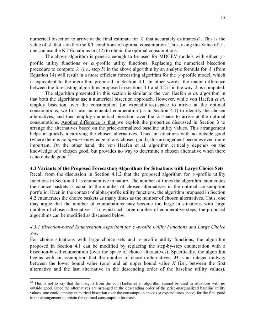
numerical bisection to arrive at the final estimate for λ that accurately estimatesE . This is the value of λ that satisfies the KT conditions of optimal consumption. Thus, using this value of λ , one can use the KT Equations in (12) to obtain the optimal consumptions.

The above algorithm is generic enough to be used for MDCEV models with either γ -profile utility functions or α -profile utility functions. Replacing the numerical bisection procedure to compute λ (i.e., step 5) in the above algorithm by an analytic formula for λ (from Equation 14) will result in a more efficient forecasting algorithm for the γ -profile model, which is equivalent to the algorithm proposed in Section 4.1. In other words, the major difference

between the forecasting algorithms proposed in sections 4.1 and 4.2 is in the way λ is computed. The algorithm presented in this section is similar to the von Haefen et al. algorithm in

that both the algorithms use a numerical bisection approach. However, while von Haefen et al. employ bisection over the consumption (or expenditures)-space to arrive at the optimal consumptions, we first use incremental enumeration (as in Section 4.1) to identify the chosen

alternatives, and then employ numerical bisection over the λ -space to arrive at the optimal consumptions. Another difference is that we exploit the properties discussed in Section 3 to arrange the alternatives based on the price-normalized baseline utility values. This arrangement helps in quickly identifying the chosen alternatives. Thus, in situations with no outside good (where there is no apriori knowledge of any chosen good), this arrangement becomes even more important. On the other hand, the von Haefen et al. algorithm critically depends on the knowledge of a chosen good, but provides no way to determine a chosen alternative when there is no outside good.12

4.3 Variants of the Proposed Forecasting Algorithms for Situations with Large Choice Sets

Recall from the discussion in Section 4.1.2 that the proposed algorithm for γ -profile utility functions in Section 4.1 is enumerative in nature. The number of times the algorithm enumerates the choice baskets is equal to the number of chosen alternatives in the optimal consumption portfolio. Even in the context of alpha-profile utility functions, the algorithm proposed in Section 4.2 enumerates the choice baskets as many times as the number of chosen alternatives. Thus, one may argue that the number of enumerations may become too large in situations with large number of chosen alternatives. To avoid such large number of enumerative steps, the proposed algorithms can be modified as discussed below.

4.3.1 Bisection-based Enumeration Algorithm for γ -profile Utility Functions and Large Choice Sets

For choice situations with large choice sets and γ -profile utility functions, the algorithm proposed in Section 4.1 can be modified by replacing the step-by-step enumeration with a bisection-based enumeration (over the space of choice alternatives). Specifically, the algorithm begins with an assumption that the number of chosen alternatives, M is an integer midway between the lower bound value (one) and an upper bound value K (i.e., between the first alternative and the last alternative in the descending order of the baseline utility values).

12 This is not to say that the insights from the von Haefen et al. algorithm cannot be used in situations with no outside good. Once the alternatives are arranged in the descending order of the price-marginalized baseline utility values, one could employ numerical bisection over the consumption space (or expenditures space) for the first good in the arrangement to obtain the optimal consumption forecasts.

16

Subsequently, based on the lambda value computed for the corresponding M, either the lower bound or the upper bound is updated to an integer midway between the previous lower and upper bounds. This process continues until a convergence is reached on the number of chosen alternatives (M) and then the optimal consumptions are computed. Thus, the proposed modifications allow the algorithm to quickly determine the chosen alternatives without the need to enumerate each (and every) chosen alternative. The detailed steps of the algorithm are provided below. Step 0: Let lower bound for M, ML = 1, let upper bound for M, MU = K. Step 1: Arrange all K alternatives available to the consumer in the descending order of their

price-normalized baseline utility values (with the outside good in the first place).

Step 2: Let M = ( ) / 2L UM M+ (i.e., an integer midway between ML and MU ).

Compute the value of λ using equation (14).

Step 3: If λ > M

Mp

ψ (i.e., the price-normalized baseline utility of alternative in position M)

Update upper bound, 1UM M= − .

Else, if λ < M

Mp

ψ (i.e., the price-normalized baseline utility of alternative in position M)

Update lower bound, LM M= .

Step 4: Compute M = ( ) / 2L UM M+ (i.e., an integer midway between ML and MU ).

Compute the value of λ using equation (14).

Step 5: If (ML < M ), go to step 3.

Else, if (ML = M ) and if λ > 1

1

M

Mp

ψ +

+

Set M = ML.

Else, if (ML = M ) and if λ < 1

1

M

Mp

ψ +

+

Set M = ML +1. Step 6: Compute the optimal consumptions using equations (15) and (16) for the first M goods

(in the arrangement of step 1). Set the consumptions of other goods as zero and stop.

4.3.2 Bisection (over the λ -space) Algorithm for α -Profile Utility Functions and Large Choice

Sets

In the case of α -profile utility functions, the algorithm proposed in Section 4.2 can be modified by avoiding the enumerative steps (i.e., steps 3 and 4 of the algorithm in section 4.2) and directly

employing a bisection-based iteration over the λ -space (as in step 5 of section 4.2). The modified algorithm is presented below. Step 0: Assume that only the outside good is chosen and let the number of chosen goods M = 1. Step 1: Arrange all the K alternatives available to the consumer in a descending order of their

price-normalized baseline utility values (with the outside good in the first place).

17

Step 2: Let 1

1

0 and L Up

ψλ λ= = , the price-normalized baseline utility of the alternative in the 1st

position.

Step 3: Step 3.1: Let ˆ ( ) / 2L Uλ λ λ= + and use Equation (19) to obtain an estimate E of E .

Step 3.2: If ( )ˆL U Eor E Eλλ λ δ δ− ≤ − ≤

Go to step 4.

Else, if E E<

Update the upper bound of λ as ( ) / 2U L Uλ λ λ= + , and go to step 3.1

Else, if E E>

Update the lower bound of λ as ( ) / 2L L Uλ λ λ= + , and go to step 3.1

Step 4: Compute the optimal consumptions of the first M alternatives in the above descending order using equations in (12). Set the consumptions of other alternatives as zero and stop.

The reader will note that this algorithm is much more similar to the von Haefen et al. algorithm than the algorithm in Section 4.2 which combines enumeration of choice alternatives

with numerical bisection over the λ -space. The only difference is that while this algorithm employs bisection over the λ -space, the von Haefen et al. algorithm employs bisection over the consumption space. Thus, one can expect both the algorithms to be computationally equivalent (i.e., provide similar computational performance).

4.4 Generalization of the Forecasting Algorithms for other KT Demand Model Systems

The algorithms developed in this section are tailored to the MDCEV model. However, similar properties as in Section 3 can be derived, and similar forecasting algorithms can be developed for other KT demand model systems in the literature with additively separable utility functions. Specifically, the basic algorithmic approach remains the same, except that some modifications may be needed depending on the form of the utility function employed in different KT demand systems, as discussed below.

• In step 1 of both the algorithms, all the K available alternatives have to be arranged in the descending order based on their marginal utility value at zero consumption. For the MDCEV model, marginal utility at zero consumption happens to be the price-normalized baseline utility. In fact, a general property of most KT demand systems used in the literature (with additively separable utility functions) is that the marginal utility at zero consumption of a chosen alternative is always greater than that of a non-chosen alternative. This property can be proved for different forms of additively separable utility functions used in the literature by following the proof of property 1 in Section 3.1.

• Similar to the above modification, in all other steps of both the algorithms, replace the price-normalized baseline utility with the corresponding marginal utility measure at zero consumption.

• Similarly, for the algorithms in Section 4.1 and 4.3.1 for γ -profile utility functions, the analytic formula for Lagrange multiplier (λ ) will depend on the form of the utility function. The formulae for optimal consumptions (conditional on the knowledge of the consumed

18

alternatives) will also depend on the form of the utility function. These formulae can be derived in a straight forward fashion following the discourse in Section 3.

In summary, the proposed algorithms are fairly generic in their approach, and can be easily modified to be used with different forms of additively separable utility functions.

5 EMPIRICAL ANALYSIS OF RESIDENTIAL ENERGY CONSUMPTION PATTERNS

In this and the next section, we estimate a model of residential energy consumption, and demonstrate the computational effectiveness and practical value of our proposed forecasting algorithms by applying it to study a variety of energy policy scenarios.

The interest in the subject of residential energy demand analysis dates back to the 1970s, reportedly beginning with the first oil crisis. This topic has gained renewed attention in recent years, due to at least three reasons. First, growing concerns regarding depleting fossil fuel resources, deteriorating environmental quality, and potentially adverse climate changes have highlighted the need for sustainable energy production and efficient energy consumption practices. Second, the residential sector is responsible for a significant share of total national-level energy consumption in many countries. For example, in the United States, the residential sector accounted for 22% of the total energy consumption during the year 2008 (EIA, 2009). Thus, analysis of residential energy consumption patterns is essential for energy planning, pricing, and policy decision-making. Third, price fluctuations, energy policies, and market conditions may result in notable welfare consequences and equity/distributional impacts. For example, Cashin and McGranahan (2006) report that low income households are likely to be impacted more than high income households due to rise in energy prices. Thus, it is important to understand energy consumption patterns in the context of price variations and policy impacts.

Section 5.1 provides an overview of the residential energy consumption studies in the past. Section 5.2 describes the RECS data used in this study, and Section 5.3 presents and discusses the MDCEV model estimation results.

5.1 Brief Overview of the Residential Energy Consumption Literature Residential energy demand analysis was initiated by the pioneering work of Houthakker (1951) on British urban electricity consumption. Since then, and especially after the oil price shocks in the 1970s, numerous studies have examined energy consumption in the residential sector, using aggregate-level econometric demand techniques (e.g., Clements and Madlener, 1999; Narayan and Smith, 2005) or disaggregate, household-level, econometric techniques. The focus in this paper is on disaggregate-household level econometric modeling techniques13. From a modeling perspective, several econometric studies use single-equation log-linear models that estimate the amount of a fuel used conditional upon a household choosing to use that fuel (e.g., Filippini and Pachauri, 2004). The approach is to regress the natural logarithm of energy consumption as a function of price, income, climate, and other variables influencing demand. Sometimes, log-log (or double-log) models, in which the explanatory variables (price, income, etc.) also take a logarithmic form along with the dependent variable, are also used (Dale et al., 2009). Log-linear and log-log models are easy to estimate and simple to interpret. For example, the coefficient of the log-price variable in a log-log model can be directly interpreted as the price elasticity of demand. However, these models have been criticized for the lack of a

13 For a recent review of econometric analyses of residential energy demand, the reader is referred to Bhattacharya and Timilisma (2009).

19

sound behavioral/ theoretical foundation (Madlener, 1996). Another stream of studies use the transcendental logarithmic (or translog) functional forms proposed by Christensen et al., (1973). The translog specification includes quadratic forms of the log-price and log-income variables in addition to first order terms in a log-log specification. This specification comes with additional flexibility relative to the log-linear or log-log models, but there is also the potential problem of obtaining unintuitive/unstable parameter (and elasticity) estimates (Madlener, 1996). Further, one cannot use single-equation regression models (whether log-linear, log-log, or translog) to simultaneously analyze households’ consumption of multiple types of fuel. Another limitation is that none of these approaches can be used to model the “discrete” choices households make on the type(s) of energy/fuel to use. On the other hand, a common feature of household energy consumption data (as will be discussed in a subsequent section) is that several households consume multiple types, but not necessarily all types, of energy available to them. This choice process can be viewed as a result of multiple discrete-continuous choices, where households make discrete choices of “whether to use” and continuous choices of “how much to use” for each type of energy available in the market.

Dubin and McFadden (1984) pioneered the joint analysis of the discrete choice of appliance holdings (choice of heating technology) and the continuous choice of energy consumption, by explicitly accounting for the self-selection effects due to unobserved factors affecting both the discrete and continuous choices. Mansur et al. (2008) use this approach for a simultaneous analysis of households’ energy/fuel type and usage choices, while Nesbakken (2001) uses the approach for a simultaneous analysis of the fuel type and usage choices for space heating.14 In such earlier studies, the discrete choice alternatives correspond to possible combinations of fuel types such as electricity only, electricity and natural gas, electricity and fuel oil, and electricity and other fuels. The continuous choice component includes the amount of consumption of each type of fuel, conditional upon the choice of fuel type combination (with self-selection terms included in the continuous choice model to account for the endogeneity of discrete choices). However, these two step estimation procedures are generally inefficient, and are also not based on a unified utility maximizing theory of multiple discreteness. Rather, they are based on exploding the fuel type combinations to generate a choice set suitable for modeling in a traditional single discrete choice framework. Even at moderate sizes of the elemental fuel type alternatives, this approach of exploding the elemental alternatives starts to generate a large number of combination alternatives for the single discrete choice (for example, 4 elemental fuel type alternatives will generate 15 combination choices of fuel types for the single discrete choice). The result is that sample sizes for estimation of such models needs to be relatively large to obtain enough households who choose each combination. On the other hand, multiple discrete-continuous KT systems handle such situations from a fundamentally unified microeconomic principle of the choice of multiple alternatives and offer an efficient framework for estimation.15 In this paper, we employ the MDCEV model in which a unified utility

14Some discrete-continuous energy demand studies also follow Hanemann’s (1984) approach in which the discrete and continuous choices are derived theoretically from the same utility maximization problem. The study by Vaage (2000), for example, belongs to this category. 15Some previous studies (e.g. Labanderia and Labeaga, 2006) have also analyzed the multi-fuel/energy usage patterns of household by employing a quadratic extension of the almost ideal demand system (AIDS) of Deaton and Muellbauer (1980) as proposed by Banks et al (1997). The AIDS system is theoretically sound, based on a unified utility maximization principle, and can be used to model the consumption of multiple types of energy/fuels in a simultaneous fashion. However, the AIDS system assumes that all types of energy are consumed by all households.

20

maximization approach for multiple discreteness is adopted to simultaneously model the “whether to consume” and “how much to consume” decisions for all types of energy.

5.2 Data

The data used in this study was obtained from the 2005 Residential Energy Consumption Survey (RECS) conducted by the Energy Information Administration (EIA) of the United States. The RECS collected a variety of information on the use of energy for a sample of 4382 households in housing units statistically selected to represent the 111.1 million housing units in the U.S. The information collected in this survey included: (1) The sources/types of energy used (electricity, natural gas, fuel oil, liquid petroleum gas (LPG), kerosene, and wood)16 and the quantity of annual consumptions and corresponding expenditures for each source/type of energy, (2) The end-uses of energy (cooking, washing/drying, heating, cooling, etc.), (3) The physical characteristics of the housing unit, (4) Information on household appliances such as space heating and cooling equipment, and (5) The demographic characteristics of the household. The information was collected from three different sources: (a) in-person interviews with householders of sampled housing units, (b) mail questionnaires or in-person/telephone interviews with rental agents of sampled rental units where some or all energy costs were included in the rent, and (c) mail questionnaires from energy suppliers who provided actual energy consumption and expenditure data for the sampled housing unit. In addition to the above-mentioned information, each household’s geographic location information was collected by the EIA, but not released to the public due to confidentiality reasons (only Census region/division information and rural/urban classifications were made available in the public use microdata). However, EIA utilized the location information to obtain weather information from the National Oceanic and Atmospheric Administration. Thus, climate variables, such as annual heating degree days and annual cooling degree days (which are described in the next section), are available in the RECS data. Further details about the survey as well as the public-use microdata used for this study are available at the following EIA website: http://www.eia.doe.gov/emeu/recs/.

Among the 4382 household records in the RECS data, several records did not contain information on the consumption of different types of energy (especially LPG consumption). Those records were supplemented by EIA with imputed consumption values and expenditures. Such imputed information, although useful for aggregate-level analysis purposes, can be inaccurate, and potentially influence the model estimates. Hence, only 2473 records with actual reported information on energy consumption and expenditures were used for model estimation. Of these 2473 households, all households consumed electricity, 59.2% (or 1465 households) consumed natural gas, 7.3% (180 households) consumed fuel oil, and 6.3% (155 households) consumed LPG.17,18

Such an assumption precludes the ability to analyze the discrete choices faced by households on the type(s) of energy to consume. The translog utility function-based model system proposed by Christensen et al. (1975) is another model that can be used to analyze multi-category energy consumption, but, like the AIDS model, assumes all types of energy are consumed. 16 Information on gasoline usage for travel purposes was not collected in this survey. 17Very few households indicated kerosene and wood consumption. Hence, the kerosene and wood alternatives were not included in the analysis. 18The implied energy consumption patterns of the 2473 households (without weighting) were not very different from

the implied consumption patterns of the 111.1 million US housing units (as obtained by expanding the original 4382 household records using weights). The only difference of relevance was in the percentage of households consuming LPG as an energy source. We chose to estimate the model with the unweighted sample of 2473 households because

21

Table 1 presents more details on the energy consumption patterns in the estimation sample (see the first set of rows in the table). As can be observed, 709 out of the 2473 households (i.e., 28.67%) consumed only electricity and no other type of fuel. All other households (i.e., 71.33% in the sample) consumed multiple types of energy (i.e., at least one other type of energy than electricity). Further, no household chose both the natural gas and LPG alternatives, indicating that these two sources of energy are perfect substitutes. In fact, all 1465 households consuming natural gas belong to the category of 1779 households that had a natural gas pipe connection to their housing unit, while all 155 LPG consuming households did not have a natural gas pipe connection to their housing unit.

The average annual household expenditure and average consumption in millions of British Thermal Units (or MBTU) in each type of energy are reported in the second set of rows in Table 1. To this data on annual energy expenditures, an additional “outside good” expenditure variable was appended (see last row in the second set of rows). The expenditure for the “outside good” for each household was computed by subtracting the household’s total annual energy expenditures (i.e., expenditures on all four types of energy – electricity, natural gas, fuel oil, and LPG) from the annual household income. Thus, for analysis purposes, households are assumed to operate with their income as a budget constraint (see Equation 3), and allocate income to consume different types of energy and to the “outside good”. The outside good includes other expenses as well as savings.

The unit prices for each type of energy are in the third set of rows.19 It can be observed that electricity is the most expensive fuel (for consumers), while natural gas is the least expensive fuel. The unit price for the outside good is set to unity. The next three sets of rows in the table provide descriptive information on the household, housing unit, and household residential location variables (in that order) used in the model. For continuous variables, the average value of that variable in the data is reported. For categorical/dummy variables, the number (and percentage) of households in the data is reported. For example, the average annual household income in the data is close to $50k. About 30% of the households belong to the low income category, while 23% belong to the high income category. Similar interpretations hold for the other household-related variables.

The climate variable group includes two variables: the annual heating degree days (HDD) and the annual cooling degree days (CDD). The HDD variable is a surrogate measure of how cold a location is over a year, relative to a base temperature of 65 degrees Fahrenheit. For each location, it is computed as the difference between the average daily temperature and 65 degrees Fahrenheit (if the average daily temperature is less than 65 degrees) summed over the 365 days in the year. Similarly, the annual cooling degree days (CDD) variable is computed as a measure

individual household imputations in the 4382-household sample may be quite different from reality, even if the aggregate consumption patterns are not very different between the 2473-housheold sample and the weighted 4382-housheold sample. 19Given the data on energy consumption and expenditures, one could potentially compute the unit price values for each type of energy consumed by each household (as expenditure divided by consumption). However, since energy prices tend to vary with consumption levels (due to block-pricing), the unit price values computed in such a fashion would be endogenous to consumption levels. Further, for any household, it is possible to compute the unit prices only for those types of energy that the household consumed, but not for non-chosen energy types. Thus, instead of computing unit price values separately for each household from the data, we used the aggregate-level unit price values given by the EIA. These values, obtained from the EIA website at the following link, vary by census divisions: http://www.eia.doe.gov/emeu/recs/recs2005/hc2005_tables/c&e/pdf/tableus7.pdf.

22

of how hot a location is over a year (relative to a base temperature of 65 degrees Fahrenheit). The use of these variables in the model allows us to study the influence of climate factors on energy consumption patterns.

5.3 Model Estimation Results

The choice alternatives in the MDCEV model include the four types of energy (electricity, natural gas, fuel oil, and LPG) and a numeraire “outside good”. We considered various estimable forms of the general utility function in Equation (2) proposed by Bhat (2008). The following form of the utility function provided the best fit to the current empirical data:

( ) ln ln ln 1 ln 1 ln 1fe n l

o o e n n f f l l

e n n f f l l

ee e eU e

p p p pψ ψ γ ψ γ ψ γ ψ

γ γ γ

= + + + + + + +

e (20)

In the above utility equation, on the right hand side, the first term ( lno otψ ) corresponds to the

utility contribution of the expenditure to the outside good, the second term corresponds to the utility contribution due to the consumption of electricity, the third, fourth and fifth terms correspond to the utility contributions due to the consumption of natural gas, fuel oil, and LPG, respectively. The subscripts, o, e, n, f, and l, used in the utility expression represent the choice alternatives of outside good, electricity, natural gas, fuel oil, and LPG, respectively.

The above utility form is obtained by constraining all the kα terms (for 1,2,3,4,5k = ) in

Equation (2) to be equal to zero (see Bhat, 2008). Further, there is no kγ term corresponding to

the outside good and electricity categories, because all households in the estimation sample allocated some non-zero amount of their income to these categories. The baseline utility terms

( kψ ) are specified as exp( )k k kzψ β ε′= + , where kz contains the observed factors (such as

household characteristics, housing unit characteristics, location attributes, and climate variables)

and kε captures the unobserved factors influencing energy consumption decisions. Further, for

identification purposes, the oψ parameter corresponding to the outside good is specified as

exp( )oε , without any observed variables kz (i.e., the outside good acts as the base alternative in

the model specification). Table 2 presents the model estimates. The baseline preference constants do not have any substantive interpretations, but capture generic tendencies to consume each type of energy as well as accommodate the range of the continuous variables in the model. However, the positive baseline preference constant for electricity (relative to the constants for other energy types) is indicative of the much higher percentage (100%) of households spending a non-zero amount of their budget on electricity relative to other energy types. The effects of other variables are discussed by variable group in the subsequent sections.

5.3.1 Household Characteristics

Among the household characteristics, annual income is specified in a logarithmic form as well as using dummy variables representing low and high income households (with medium income as the base for the dummy variable specification). The negative coefficient on the log(income) variable indicates that the proportion of household income (but not necessarily the absolute dollar amount) spent on energy consumption decreases with increasing income levels. This impact is further reinforced by the positive coefficient on the low income dummy variable, (though this dummy variable effect is only marginally significant). A direct policy implication of

23

these results is that energy price increases have larger welfare impacts on low income households than other households (see Cashin and and McGranahan, 2006). Also, according to the estimated coefficient on the high income dummy variable, high income households, in general, expend a higher share of their income (when compared to low income households) on electricity. This is perhaps because high income households tend to own and use a wider variety and a larger number of electric-operated appliances.

The household size (i.e., number of people in household) related coefficients indicate that larger household sizes are associated with higher energy consumption, in the context of electricity and natural gas. The log(householder age) variable refers to the natural logarithm of the age of the householder.20 The estimated effects of this variable imply that households at an older stage in their lifecycle are more pre-disposed to use non-electricity type of fuels (natural gas, fuel oil, and LPG) relative to electricity.

5.3.2. Housing Unit Characteristics

The coefficients on the log(age of housing unit) variable indicate that households living in older houses are more likely to use fuel oil and natural gas than those living in newer houses. This result corresponding to fuel oil is consistent with the declining popularity of fuel oil as a heating source, due to the extensive maintenance needs and environmental and health risks associated with fuel oil heaters and tanks. The result corresponding to natural gas is consistent with the trend that natural gas consumptions in the U.S. have declined over the years, perhaps due to two reasons (AGA 2003): (1) the increased efficiency of natural gas appliances such as space heaters and water heaters, and better insulation features and energy efficiency of newer houses, and (2) the reduction in the number of gas appliances in homes served with gas.

As expected, households living in larger houses (in terms of house area) expend more on energy relative to households living in smaller houses. They are also more likely (than those in smaller houses) to use fuels other than electricity, such as natural gas, fuel oil, and LPG. It is likely that owners of smaller houses (with lower energy needs) are less likely to choose non-electricity types of fuels due to higher capital costs of installing equipment for such fuels as natural gas and fuel oil. On the other hand, as energy needs increase, it is likely that households choose fuels with lower prices and hence higher returns to off-set the capital costs (see Mansur et al., 2008 for similar findings). Recall from Table 1 that the unit price of electricity is much higher than that of other fuels.

Households in multifamily units are associated with lower energy consumptions than those in single family dwelling units and mobile homes. This may be attributable to the lower heating and other energy requirements due to such features as shared walls in multifamily units.

The final variable among housing unit characteristics corresponds to the availability of a natural gas pipe connection to the house. As indicated earlier, a household’s choice between the natural gas and LPG alternatives depended on the availability of a natural gas pipe connection to its house. Further, no household chose both natural gas and LPG alternatives. Our model specification accommodates such perfect substitutability between the two alternatives by deterministically making the natural gas option available only to those houses with a natural gas pipe connection, and the LPG option available only to those houses without a natural gas pipe connection. Besides such availability constraints in the context of natural gas and LPG fuels, the 20According to the EIA, the householder is defined as the person who lives in the housing unit and in whose name the house is owned or rented. If the house owner (or the renter) does not live in the housing unit, the householder is defined as the person responsible for paying the household bills.

24

availability of a natural gas pipe connection also impacts the choice and consumption of other fuels. As expected, the presence of a natural gas pipeline decreases the energy expenditure on electricity and fuel oil.

5.3.3 Household Location Characteristics

Households in rural locations are less likely to choose natural gas, but are more likely to choose LPG. This result may be due to the lower connectivity of natural gas utilities to rural locations. Also, households in southern regions appear to be less likely to opt for natural gas, while those in the north-eastern region are highly reliant upon fuel oil, a well established trend (EIA, 2008).

5.3.4. Climate Variables

The coefficients corresponding to the log(HDD) and log(CDD) variables indicate that households in colder climates expend more income share on energy than those in other climates, except for those households in very hot climates. These latter households expend more income share on electricity than households in other climates. These results are quite intuitive. Households in cold climates have increased space heating needs, leading to an increase in energy share expenditure in general, and in non-electricity types of fuels in particular (space heaters generally use non-electricity sources of energy). On the other hand, households in very hot climates have space cooling needs, and air-conditioning units predominantly use electricity as the source of energy. In summary, the climate variable effects indicate that households in cold climates are more likely to use fuel oil, natural gas, and LPG, while those in hot climates tend to consume higher amounts of electricity.21

5.3.5. Satiation and Scale Parameters

The next set of parameters corresponds to the kγ terms. As discussed earlier, there is no such

term corresponding to the electricity alternative because all households consume a non-zero

amount of electricity (hence, no need for corner solutions). The kγ terms for other fuels are all

significantly different from zero, indicating the possibility of corner solutions (i.e., zero consumption) for some households.

Finally, since there is variation in the unit prices ( kp ) across the energy/fuel choice

alternatives, we could estimate the scale parameter associated with the Gumbel distribution of

the baseline utility functions ( kψ ) without assuming it to be unity (see Bhat, 2008). The scale

parameter can be interpreted as a measure of the magnitude of unobserved factors influencing the

baseline utility functions ( kψ ). In a naïve MDCEV model with only constants in the baseline

21A caveat is in order here regarding the annual HDD and CDD variables. These variables are good measures of space heating and cooling needs, respectively. However, they may not unambiguously represent the seasonal temperature variations at a location. This is because the degree-days measure does not distinguish between a large number of moderately high/low temperatures and a small number of extremely high/low temperatures. Further, since the variables are constructed using 65 degrees Fahrenheit as the base temperature, there is an inherent assumption that 65 degrees Fahrenheit is the optimum temperature (at which least amount of energy is consumed). Using detailed information on temperature variations across different seasons (e.g., winter temperatures and summer temperatures) in the model may overcome these limitations and provide better insights into climate effects on energy consumption. However, the RECS data available for public use does not contain such information. Even the geographic location information is available at a coarse geography such as census region and division variables, rural/urban variables, and states. At the least, county-level geographic location information is required to be able to merge detailed temperature data from other sources in to the RECS database. Mansur et al. (2008) include such detailed temperature information in their energy consumptions analysis.

25

utility functions, and satiation parameters (i.e., a model with no other covariates), the scale parameter was estimated to be 0.608 (not shown in tables). As more and more explanatory variables were specified in the baseline utility functions, the magnitude of the scale parameter estimate decreased. In the final model specification (as shown in Table 2), the scale parameter estimate is 0.331. The decrease in magnitude of the scale parameter estimate from 0.608 for the naïve model to 0.331 for the final specification indicates that the specified explanatory variables capture about 46% of the variation in the logarithm of households’ preferences toward different energy alternatives. This predictive value of the model is also corroborated by log-likelihood measures of fit. Specifically, the log-likelihood for the naïve MDCEV specification is -36823.5, while that for the final MDCEV specification with 26 additional parameters is -34549.5. The likelihood ratio statistic between the two specifications is 4548, which is substantially higher than the critical chi square value for 26 degrees of freedom at any level of significance. Overall, the MDCEV model estimates are consistent with expectations and shed light on the influence of different household, housing unit, location, and climate characteristics on residential energy consumption patterns. In the next section, we use these model estimates and the proposed forecasting procedure to examine various policy scenarios.

6 PREDICTION EXPERIMENTS AND SCENARIO ANALYSIS

In this section, we first present prediction experiments with the RECS data to assess the computational time performance of the proposed forecasting algorithms in the current empirical context (Section 6.1). For further assessment in choice situations with large choice sets, we present additional prediction experiments with simulated datasets in Section 6.2. Next, we conduct policy simulations to predict the impact of different climate change scenarios and other scenarios on residential energy consumption patterns in the U.S. (Section 6.3).

6.1 Computational Time Analysis of the Proposed Forecasting Algorithms (with the RECS

data)

To assess the computational performance of the proposed forecasting algorithms (presented in Sections 4.1 and 4.2), several prediction experiments were undertaken with different samples of the 4382-household data, varying from 1000 households to the full-RECS sample of 4382 households.22 To recognize stochasticity, in each experiment, predictions were carried out

repeatedly using several sets of draws of the kε terms, varying from 100 sets to 500 sets for each household. Specifically, scrambled Halton sequences (Bhat 2003) of standard uniform distributions were generated and converted into Gumbel distributions with the scale parameter as estimated in the model and the location parameter as zero.

For all prediction exercises, both the proposed forecasting procedures from Sections 4.1 and 4.2 were coded and executed in the Gauss matrix programming language. In addition, for comparison purposes, the gradient-based constrained optimization routines of the Constrained Maximum Likelihood (CML) module of Gauss were used to undertake the same prediction exercises.23 Further, the numerical bisection algorithm of von Haefen et al. (2004) was also

22Although the model estimation was pursued with the sample of 2473 household records containing exogenous

energy consumption/expenditure information, forecasting exercises were conducted with the full survey sample of 4382 households. This enables us to directly use the population weights to expand the RECS sample to the population of 111.1 million housing units in the U.S. 23

The CML module of Gauss uses a sequential programming method for constrained non-linear optimization, in

which the optimal values are approximated iteratively using the gradients of the Lagrangian function.

26

coded in Gauss and used to assess its performance vis-à-vis the algorithms proposed in this paper and the gradient-based CML routines of Gauss. All predictions were performed with a desktop computer of 2.66GHz processing speed and 3.25GB Random Access Memory (RAM). Table 3 shows the computation times of the forecasting algorithms proposed in Sections 4.1 and 4.2 of this paper, as well as those of the von Haefen et al. algorithm and the gradient-based CML module of Gauss. In this table, the computation times reported in the first block of rows correspond to prediction runs of the incremental enumeration algorithm proposed in this

paper for γ -profile utility functions (i.e., the algorithm proposed in Section 4.1) on datasets of different sample sizes and with different sets of error term draws. For example, to predict the energy expenditures/consumptions of 4382 households, hundred different times for each household (each time with a different set of error term draws), the proposed incremental enumeration algorithm took only 10.62 seconds (see last column). Another observation from the table is that the computation time increases almost linearly with the number of households (across the columns in each row) as well as with the number of sets of error term draws (across the rows in each column). Nevertheless, even for the entire dataset of 4382 households, and with 500 sets of error term draws for each household, the total computation time is less than a minute.

The next set of rows in the table shows the computation times for the second forecasting algorithm proposed in this paper (in Section 4.2), which is designed for general utility functions

that do not restrict the kα parameters to be equal across alternatives. These computation times

are at least 4 times longer than those of the algorithm designed specifically for γ -profile utility functions. The increase in computation time is because the general algorithm adopts an iterative

approach to determine the value of the Lagrange multiplierλ , while the algorithm designed for γ -profile utility functions obviates the need for iterations by using an analytic expression for λ .

The third set of rows in the table shows the computation times for the von Haefen et al. (2004) algorithm. These computation times are about 14 times (3 times) longer than those of the

algorithm proposed in this paper for γ -profile utility functions (more general utility functions). These run time differences highlight the efficiency of the algorithms proposed in this paper,

especially the algorithm designed for γ -profile utility functions. The final block of Table 3 shows the computational performance of the gradients-based,

iterative constrained optimization routine (available in the CML module of Gauss). As can be observed, to compute the expenditure patterns of 4382 households for just one set of error term draws for each household, it took 3 hours and 36 minutes. A linear extrapolation to 100 sets of error term draws implies a rather large computation time of about 15 days. These long run times clearly highlight the inefficiency of the gradient-based, iterative algorithm. To be sure, we could reduce the computation time of the gradient-based algorithm by easing its convergence criteria. But this resulted in suboptimal solutions for a large number of households. In fact, even at the convergence criteria that resulted in the reported computation times of 15 days, the predicted expenditures for some households were suboptimal. Specifically, non-negligible differences were found between the predicted expenditures of the gradients-based procedure and that of the proposed procedure for a small number of households. In such cases, the utility values corresponding to the predictions from the proposed algorithms were higher compared to that of the iterative procedure, indicating that the gradient-based algorithm resulted in suboptimal solutions. As the convergence criteria were tightened to improve the accuracy of the results (i.e., to obtain more optimal solutions), the computation time increased considerably. In all fairness to

27

the gradient-based iterative algorithm, perhaps such a level of accuracy is not necessary for practical purposes. However, as the convergence criteria were eased to reduce the computation time to a day (as opposed to 15 days), the quality of the results deteriorated too much to be of practical value. Thus, there seems to be a clear trade-off between accuracy and computation time that the analyst has to make, when using a gradient-based algorithm. Even after making the trade-off, the analyst is left with an undesirable amount of computation time (in the order of days) for just one prediction exercise (with 4382 households and 100 sets of error term draws).

The incremental enumeration algorithm we propose for the γ -profile utility functions, on the other hand, is analytic in nature and does not leave room for any approximations or inaccuracy, and is free from any trade-off between accuracy and computational efficiency.24 Finally, in certain (although a small number of) instances with tight convergence criteria, the gradient-based procedure ran into convergence problems, requiring forced termination and resulting in suboptimal solutions. On the other hand, both the algorithms proposed in this paper as well as the von Haefen et al. algorithm did not run into convergence issues.

To further demonstrate the computational efficiency of the proposed algorithms, we undertook predictions with different sets of bootstrapped parameter estimates (obtained based on the covariance matrix of the model estimates). For example, as discussed earlier, for the entire dataset of 4382 households, with 100 sets of error term draws, but only one set of parameter estimates, the computation time was 10.62 seconds for the incremental enumeration algorithm

we designed (in Section 4.1) for γ -profile utility functions. When predictions were carried out with the same dataset and the same number of error term draws, but with 50 sets of bootstrapped parameter estimates, the computation time was about 8 and half minutes (510 seconds). With 100 sets of bootstrapped parameter estimates, the computation time was about 17 minutes (1019 seconds), which is not an unreasonable amount of time. To do the same, the other algorithm proposed in this paper (for more general utility functions; Section 4.2) took about 38 minutes for 50 bootstrapping repetitions and 76 minutes for 100 bootstrapping repetitions. The von Haefen et al. algorithm took about 2 hours for 50 bootstrapping repetitions and 4 hours for 100 bootstrapping repetitions. On the other hand, the gradient-based, iterative algorithm would need an unreasonably large amount of time to do the same (it would need more than a year with 50 sets of bootstrapped estimates!).

It can be observed that the ratios of the above-reported run-times are similar to the ratios

discussed earlier in this section. That is, the proposed incremental enumeration algorithm for γ -profile utility functions is about 4 times faster than the proposed algorithm in Section 4.2

(incremental enumeration combined with bisection over λ -space), and about 14 times faster than the von Haefen et al. algorithm. Similarly, the proposed algorithm in Section 4.2 is at least 3 times faster than the von Haefen et al. algorithm. Such computational efficiencies become crucial in application contexts with a large number of agents and when bootstrapping is needed to compute standard errors of the predictions, as is usually the case with travel demand and other microsimulation models.

24

The other algorithm we propose (for general utility functions) as well as the von Haefen et al. algorithm are also

associated with similar trade-offs between accuracy and computational efficiency, because of the iterative nature of these algorithms. For example, the accuracy of the von Haefen et al. algorithm could be increased in the decimal places of the predicted expenditures by tightening the convergence criteria that increased the run times to one-and-half times the run times reported in Table 3.

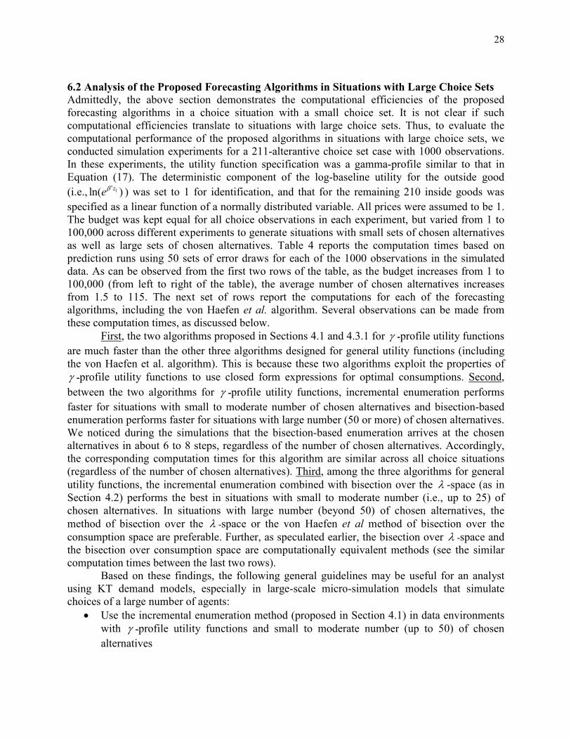
28

6.2 Analysis of the Proposed Forecasting Algorithms in Situations with Large Choice Sets

Admittedly, the above section demonstrates the computational efficiencies of the proposed forecasting algorithms in a choice situation with a small choice set. It is not clear if such computational efficiencies translate to situations with large choice sets. Thus, to evaluate the computational performance of the proposed algorithms in situations with large choice sets, we conducted simulation experiments for a 211-alterantive choice set case with 1000 observations. In these experiments, the utility function specification was a gamma-profile similar to that in Equation (17). The deterministic component of the log-baseline utility for the outside good

(i.e., 1ln( )zeβ ′) was set to 1 for identification, and that for the remaining 210 inside goods was

specified as a linear function of a normally distributed variable. All prices were assumed to be 1. The budget was kept equal for all choice observations in each experiment, but varied from 1 to 100,000 across different experiments to generate situations with small sets of chosen alternatives as well as large sets of chosen alternatives. Table 4 reports the computation times based on prediction runs using 50 sets of error draws for each of the 1000 observations in the simulated data. As can be observed from the first two rows of the table, as the budget increases from 1 to 100,000 (from left to right of the table), the average number of chosen alternatives increases from 1.5 to 115. The next set of rows report the computations for each of the forecasting algorithms, including the von Haefen et al. algorithm. Several observations can be made from these computation times, as discussed below.

First, the two algorithms proposed in Sections 4.1 and 4.3.1 for γ -profile utility functions are much faster than the other three algorithms designed for general utility functions (including the von Haefen et al. algorithm). This is because these two algorithms exploit the properties of

γ -profile utility functions to use closed form expressions for optimal consumptions. Second, between the two algorithms for γ -profile utility functions, incremental enumeration performs faster for situations with small to moderate number of chosen alternatives and bisection-based enumeration performs faster for situations with large number (50 or more) of chosen alternatives. We noticed during the simulations that the bisection-based enumeration arrives at the chosen alternatives in about 6 to 8 steps, regardless of the number of chosen alternatives. Accordingly, the corresponding computation times for this algorithm are similar across all choice situations (regardless of the number of chosen alternatives). Third, among the three algorithms for general

utility functions, the incremental enumeration combined with bisection over the λ -space (as in Section 4.2) performs the best in situations with small to moderate number (i.e., up to 25) of chosen alternatives. In situations with large number (beyond 50) of chosen alternatives, the

method of bisection over the λ -space or the von Haefen et al method of bisection over the consumption space are preferable. Further, as speculated earlier, the bisection over λ -space and the bisection over consumption space are computationally equivalent methods (see the similar computation times between the last two rows). Based on these findings, the following general guidelines may be useful for an analyst using KT demand models, especially in large-scale micro-simulation models that simulate choices of a large number of agents:

• Use the incremental enumeration method (proposed in Section 4.1) in data environments with γ -profile utility functions and small to moderate number (up to 50) of chosen alternatives

29

• Use the bisection-based enumeration method (proposed in Section 4.3.1) in data environments with γ -profile utility functions and large (more than 50) number of chosen alternatives

• Use incremental enumeration combined with bisection over the λ -space (as in Section 4.2) in data environments with α -profile utility functions and small to moderate number (up to 50) of chosen alternatives

• Use either the proposed bisection over λ -space (as in Section 4.3.2) or von Haefen et al.’s bisection over consumption-space in data environments with α -profile utility functions and large number (more than 50) of chosen alternatives

6.3 Scenario Analysis

This section presents the results of several policy simulations to assess the impact of four different scenarios on residential energy consumption/expenditure patterns in the U.S. Two of the four scenarios are related to climate change: (1) A 450 degree Fahrenheit increase in annual cooling degree days, and (2) A 450 degree Fahrenheit increase in annual heating degree days. These scenarios can be viewed as a result of a 5o Fahrenheit rise (for the first scenario) or a 5o Fahrenheit drop (for the second scenario) in average daily temperature from 65o for 3 months (90 days) in a year. The other two scenarios are related to the size of housing units in the U.S.: (1) A 10% increase in the floor area of all houses, and (2) a 10% decrease in the floor area of all houses. The predictions were carried out for 50 sets of bootstrapped parameter estimates. For each set of parameter estimates, 100 sets of error term draws were used for each household to simulate unobserved heterogeneity. The prediction results are presented in Tables 5, 6, and 7, each of which is discussed next.

Table 5 presents the predicted residential energy expenditures as well as the observed expenditures for the base case scenario (the standard errors of the predictions are in parenthesis, and are obtained from bootstrapping). The first two numeric columns (under the label of “sample predictions”) of the table show the average predicted energy expenditures and consumptions, averaged over all households, all sets of bootstrapped model parameters, and all sets of error term draws, for the sample data set. The third and fourth numeric columns (under the label of “sample observations”) show the observed average (over all households) energy expenditures and consumptions in the sample data. For example, the model predicts that, on average, a household spends $1100 per annum to consume 38 Million British Thermal Units (MBTU) of electricity, while the observed average household expenditure on electricity is $1116 per annum (for 39 MBTU). It can be observed that the aggregate predictions are reasonably close to the observed energy expenditures and consumptions25, except a notable discrepancy in the context of natural gas consumption (the model seems to be over-predicting natural gas consumption). The weights available in the data were used to expand the predicted (and observed) expenditures and consumptions to total annual energy expenditures and consumptions for all the 111.1 Million housing units in the U.S. Such population totals are shown in the second half of Table 5, under

25

Although the predictions appear close to the observed expenditures, we do not claim this as a validation of the

model. This is because at least half of the sample (over which predictions were performed) includes the estimation data. Showing that the model closely predicts aggregate-level statistics in the estimation sample is not a sufficient yardstick for model performance. Besides, what is more important is appropriate sensitivity of the model to relevant policies and changes in the explanatory variables.

30

“population predictions” and “population observations”. Similar predictions were obtained for all the above-mentioned four scenarios, as discussed next.

Table 6 shows the predictions for the two climate change scenarios. The first two numeric columns of the table contain the predicted changes in residential energy expenditure and consumption patterns due to a 450 degree Fahrenheit increase in annual cooling degree days (CDD). Both average predicted changes and standard errors (obtained from bootstrapping) are reported in the table, with the standard errors in parentheses. According to these predictions, due to a 450 degree Fahrenheit increase in annual CDD, the overall residential electricity energy expenditure in the U.S. would increase by $5.581 Billion. This is due to an increase in electricity consumption by 189.78 Trillion BTU, which is equivalent to 55.66 Billion Kilo Watt Hours (KWH) of additional electricity. It can also be observed from the results that most of the increase in expenditures due to additional electricity consumption is drawn from the “outside good” which includes other household expenditures and savings. These results indicate severe welfare impacts of climate warming. The third and fourth numeric columns in Table 6 present the predicted changes in residential energy expenditure and consumption patterns due to a 450 degree Fahrenheit increase in annual heating degree days (HDD). The model predictions indicate an overall increase in residential energy expenditures by $5.104 Billion, most of which is due to increased consumption of natural gas (by 191.48 Trillion BTU) and fuel oil (by 116.06 Trillion BTU). This is an expected result because space heating requirements increase at cooler temperatures, and natural gas and fuel oil are primarily used for space heating purposes. Table 7 presents the predicted energy expenditure and consumption changes for scenarios related to the size of houses in the U.S. Specifically, it is predicted that a 10% increase in the floor area of all houses in the U.S. leads to an increase in residential energy expenditures by $4.741 Billion. A large part of this increase is due to increased consumption of natural gas (by 110.93 Trillion BTU), electricity (by 84.39 Trillion BTU), and fuel oil (by 54.10 Trillion BTU). On the other hand, if the houses were 10% smaller in size, the residential energy expenditures would decrease by $5.117 Billion. These savings would result primarily from reduced consumption of natural gas and electricity, followed by fuel oil.

7 SUMMARY AND CONCLUSIONS

In this paper, we propose simple and computationally efficient forecasting algorithms for the MDCEV model. These algorithms build on simple, yet insightful, analytic explorations of the Kuhn-Tucker conditions of optimality that shed new light on the properties of the model. For

specific forms of the consumption utility function (i.e., a γ -profile utility function), the algorithm obviates the need to undertake any iterative constrained optimization procedures that have hitherto been used for forecasting with Kuhn-Tucker (KT) demand system models. The non-iterative nature of the algorithm contributes significantly to its efficiency and accuracy. Even with more general utility functions that fall within the class of additively separable utility functions, we use the properties of the MDCEV model to design efficient (albeit iterative) forecasting algorithms. We also propose variants of the proposed algorithms that perform faster in situations with large choice sets. Further, although developed in the context of the MDCEV model, the proposed algorithms can easily be modified for use with other utility maximization-based Kuhn-Tucker (KT) consumer demand model systems with additively separable utility functions.

31

To demonstrate the effectiveness of the forecasting algorithms, we present an analysis of residential energy consumption patterns in the U.S. using the MDCEV model and its forecasting algorithm proposed in this paper. Household-level energy consumption data from the 2005 Residential Energy Consumption Survey (RECS) conducted by the Energy Information Administration (EIA) was utilized for this analysis. The MDCEV model estimates provide insights into the influence of household, house-related, residential location, and climatic factors on households’ consumption patterns of different types of energy, including electricity, natural gas, fuel oil, and liquefied petroleum gas (LPG).

Prediction exercises with the proposed algorithms, a numerical bisection-based iterative algorithm proposed by von Haefen et al. (2004), and a general gradient-based iterative algorithm indicate the significant computational efficiency (as well as accuracy) of the proposed algorithms. In the current empirical context, to predict the energy consumption patterns of 4382 households, with 100 sets of error term draws for each household, the incremental enumeration

algorithm proposed for γ -profile utility functions took only 11 seconds. On the other hand, the von Haefen et al. procedure took 143 seconds, and the gradient-based, iterative forecasting routine would take around 15 days to do so. Even when the predictions were conducted over as

much as 50 sets of bootstrapped parameter estimates, the algorithm proposed for γ -profile utility functions took only about 8 and half minutes, while it took about 2 hours to accomplish this with the von Haefen et al. algorithm, and it would take about a year to do the same with the gradients-based iterative algorithm. Further prediction exercises on simulated data with large choice sets

suggest the following general guidelines. (1) For γ -profile utility functions, incremental enumeration performs well in choice situations with small to moderate number (up to 50) of chosen alternatives, while bisection-based enumeration performs well in choice situations with

large number (beyond 50) of chosen alternatives. (2) For α -profile utility functions, incremental enumeration combined with bisection over the λ -space performs well in situations with small to moderate number of chosen alternatives, while a simple bisection over the λ -space or over the consumption-space (as in von Haefen et al., 2004) perform well in situations with large number of chosen alternatives.

The computational efficiencies of the proposed algorithms facilitated policy simulations to predict the impact of climate change and other scenarios on residential energy consumption patterns. The results indicate that a 450 degree Fahrenheit increase in cooling degree days over a year can lead to a $5.581 Billion increase in residential expenditures on electricity. This is due to 55.66 Billion Kilo Watt Hours (KWH) of additional electricity consumption. Similarly, a 450 degree Fahrenheit increase in cooling degree days over a year can lead to a $5.104 Billion increase in residential energy expenditures, primarily due to increased consumption of natural gas and fuel oil. In the context of house sizes in the U.S., if the houses were 10% smaller (larger) in their floor area, the residential energy expenditures would decrease (increase) by $5.117 Billion ($4.741 Billon).

The effectiveness of the proposed algorithms for forecasting and policy analysis with MDCEV and other KT demand model systems should facilitate the increased use of these model systems in applied research and policy analysis. In fact, one of the proposed algorithms is now being used in a large-scale activity-based travel demand micro-simulation system for predicting the vehicle ownership/usage and activity-participation and time-use patterns of individuals in the Los Angeles area (with a population of about 20 million individuals). Another useful application of this algorithm is that it can be used to quickly generate large sets of synthetic data for

32

simulation experiments to understand the properties of MDCEV and other KT demand model systems. For example, now that a fast and easy-to-use forecasting procedure is available, further research can be conducted to characterize the distributions of forecasts obtained from KT demand systems. Besides, one can conduct predictive validation assessments of the MDCEV approach for different empirical contexts (see Jaggi and Axhausen, 2011 for a recent effort).

Future studies would benefit from explicitly accommodating the potential endogeneity of energy prices in energy consumption (due to block pricing). Another extension is to include gasoline consumption (for travel needs) in the analysis. Including temperature and other weather variables at a fine space and time resolution is another useful direction for extending the current empirical analysis. On the methodological front, there is an important need to develop similarly easy forecasting approaches for KT demand models that allow flexible, non-additive utility functions.

33

REFERENCES

Ahn, J., Jeong, G., and K. Yeonbae (2007) A forecast of household ownership and use of alternative fuel vehicles: A multiple discrete-continuous choice approach. Energy Economics, 30(5), 2091-2104.

AGA/American gas Association (2003) Patterns in residential natural gas consumption, 1997-2001.

Banks, J., Blundell, R. W. and Lewbel, A. (1997) Quadratic Engel curves, indirect tax reform and welfare measurement. Review of Economics and Statistics, 79, 527–39.

Bhat, C.R. (2003) Simulation Estimation of Mixed Discrete Choice Models Using Randomized and Scrambled Halton Sequences. Transportation Research Part B, 37(9), 837-855.

Bhat, C.R. (2005) A Multiple Discrete-Continuous Extreme Value Model: Formulation and Application to Discretionary Time-Use Decisions. Transportation Research-B, 39(8) 679-707.

Bhat, C.R. (2008) The Multiple Discrete-Continuous Extreme Value (MDCEV) Model: Role of Utility Function Parameters, Identification Considerations, and Model Extensions. Transportation Research-B, 42(3), 274-303.

Bhat, C.R., S. Sen, and N. Eluru (2008). The Impact of Demographics, Built Environment Attributes, Vehicle Characteristics, and Gasoline Prices on Household Vehicle Holdings and Use. Transportation Research-B, 43(1) 1-18.

Bhattacharyya, S.C., and G.R. Timilsina (2009) Energy Demand Models for Policy Formulation: A Comparative Study of Energy Demand Models. Working Paper No. 4866, Development Research Group of The World Bank, March 2009.

Cashin, D.B, and L. McGranahan (2006) Household energy expenditures, 1982–2005. Chicago Fed Letter, Federal Reserve Bank of Chicago, June 2006.

Christensen, L., Jorgenson, D., and L. Lawrence (1973) Transcendental Logarithmic Production Frontiers. The Review of Economics and Statistics, 55, 28-45.

Christensen, L., Jorgenson, D., and L. Lawrence (1975) Transcendental Logarithmic Utility Functions. The American Economic Review, 65, 367-83.

Clements, M. P. and R. Madlener (1999) Seasonality, cointegration and forecasting UK residential energy demand. Scottish Journal of Political Economy, 46(2), 185-206.

Dale, L., K.S. Fujita, F.V. Lavín, M. Moezzi, M. Hanemann, S. Guerrero, and L. Lutzenhiser (2009) Price Impact on the Demand for Water and Energy in California Residences. California Climate Change Center, August 2009.

Deaton, A. S. and Muellbauer, J. N. J. (1980), ‘An Almost Ideal Demand System’, American Economic Review, 70, 312–26.

Dubin, J.A., McFadden, D.L. (1984) An econometric analysis of residential electric appliance holdings and consumption. Econometrica, 52, 118-131.

EIA (2008) “Residential Heating Oil Prices: What Consumers Should Know” EIA Brochure #: DOE/EIA-X048, released December 2008, retrieved June 1, 2010 from the EIA Website.

EIA (2009) Annual Energy Review 2008. Report prepared by the Energy Information Administration, Office of Markets and End Use, U.S. Department of Energy, Washington DC. June 2009. www.eia.doe.gov/aer

Fang, H.A. (2008). A discrete–continuous model of households’ vehicle choice and usage, with

an application to the effects of residential density. Transportation Research Part B 42(9),

736-758.

34

Ferdous, N., Pinjari A.R., Bhat C.R., and R.M. Pendyala (2010). A comprehensive analysis of household transportation expenditures relative to other goods and services: an application to United States consumer expenditure data. Transportation, 37(3), 363-390.

Filippini, M. and S. Pachauri (2004) Elasticities of electricity demand in urban Indian households. Energy Policy, 32, 429-36.

Habib, K. M. N., Miller, E. J. (2009) Modeling Activity Generation: A Utility-based Model for Activity Agenda Formation. Transportmetrica 5(1), 3-23.

Hanemann, W.M. (1978). A methodological and empirical study of the recreation benefits from water quality improvement. Ph.D. dissertation, Department of Economics, Harvard University.

Hanemann, W.M. (1984) Discrete/continuous models of consumer demand. Econometrica 52, 541-561.

Houthakker, H.S. (1951) Some Calculations of Electricity Consumption in Great Britain. Journal of the Royal Statistical Society. Series A, 114 (3), 351-371.

Kim, J., G.M. Allenby, and P.E. Rossi (2002). Modeling consumer demand for variety. Marketing Science, 21, 229-250.

Labandeira, X. and Labeaga, J.M. (1999) Combining Input–Output Analysis and Micro-Simulation to Assess the Effects of Carbon Taxation on Spanish Households. Fiscal Studies, 20 (3), 305–320.

Liao, H.C. and T. F. Chang (2002) Space-heating and water-heating energy demands of the aged in the US. Energy Economics, 24, 267-84.

Madlener, R (1996). Econometric Analysis of Residential Energy Demand: A Survey. Journal of Energy Literature. 2(2), 3-32.

Mansur, E.T., R. Mendelsohn, and W. Morrison (2008) Climate change adaptation: A study of fuel choice and consumption in the US energy sector. Journal of Environmental Economics and Management, 55, 175–193.

Narayan, P. K. and R. Smyth (2005) The residential demand for electricity in Australia: an application of the bounds testing approach to cointegration, Energy Policy, 33, 467-74.

Nesbakken, R (2001) Energy Consumption for Space Heating: A Discrete-Continuous Approach. Scandinavian Journal of Economics. 103 (1), 165-184.

Phaneuf, D.J., Kling, C.L., and Herriges, J.A., 2000. Estimation and welfare calculations in a generalized corner solution model with an application to recreation demand. The Review of Economics and Statistics, 82(1), 83-92.

Pinjari, A.R., Bhat, C.R., and Hensher, D.A. (2009) Residential Self-Selection Effects in an Activity Time-use Behavior Model. Transportation Research Part B, 43(7), 729-748.

Pinjari, A.R. (2011) Generalized Extreme Value (GEV)-based Error Structures for Multiple Discrete-Continuous Choice Models. Technical Paper. Department of Civil and Environmental Engineering, University of South Florida.

Pinjari, A.R., and C.R. Bhat (2010) A Multiple Discrete-Continuous Nested Extreme Value Model: Formulation and Application to Non-Worker Activity Time-use and Timing Behavior on Weekdays. Transportation Research Part B, 44(4), 562-583.

Rajagopalan, B.S., and K.S., Srinivasan (2008) Integrating Household-Level Mode Choice and Modal Expenditure Decisions in a Developing Country: Multiple Discrete-Continuous Extreme Value Model. Transportation Research Record, No. 2076, 41-51.

35

Rajagopalan, B.S., Pinjari, A.R., and C.R. Bhat (2008) A Comprehensive Model of Worker’s Non-work Activity Time-use and Timing Behavior. Forthcoming, Transportation Research Record.

Srinivasan, S., and C.R. Bhat (2006). A Multiple Discrete-Continuous Model for Independent- and Joint- Discretionary-Activity Participation Decisions. Transportation, 33(5), 497-515.

Vaage, K (2000) Heating technology and energy use: a discrete/continuous choice approach to Norwegian household energy demand. Energy Economics, 22, 649–666.

Vasquez-Lavin, F., and M. Hanemann (2009) Functional Forms in Discrete/Continuous Choice Models with General Corner Solutions. Proceedings of the 1st International Choice Modeling Conference, Harrogate, March 2009.

von Haefen, R.H. (2003) Incorporating observed choice into the construction of welfare measures from random utility models. Journal of Environmental Economics & Management, 45(2), 145-165.

von Haefen, R.H., Phaneuf, D.J., and Parsons, G.R. (2004) Estimation and welfare analysis with large demand systems. Journal of Business and Economic Statistics, 22(2), 194-205.

von Haefen, R.H., and D.J. Phaneuf (2005) Kuhn-Tucker Demand System Approaches to Nonmarket Valuation, in R. Scarpa and A.A. Alberini (Eds.), Applications of Simulation Methods in Environmental and Resource Economics, Springer.

Wales, T.J., and Woodland, A.D. (1983) Estimation of Consumer Demand Systems with Binding Non-Negativity Constraints. Journal of Econometrics, 21(3), 263-85.

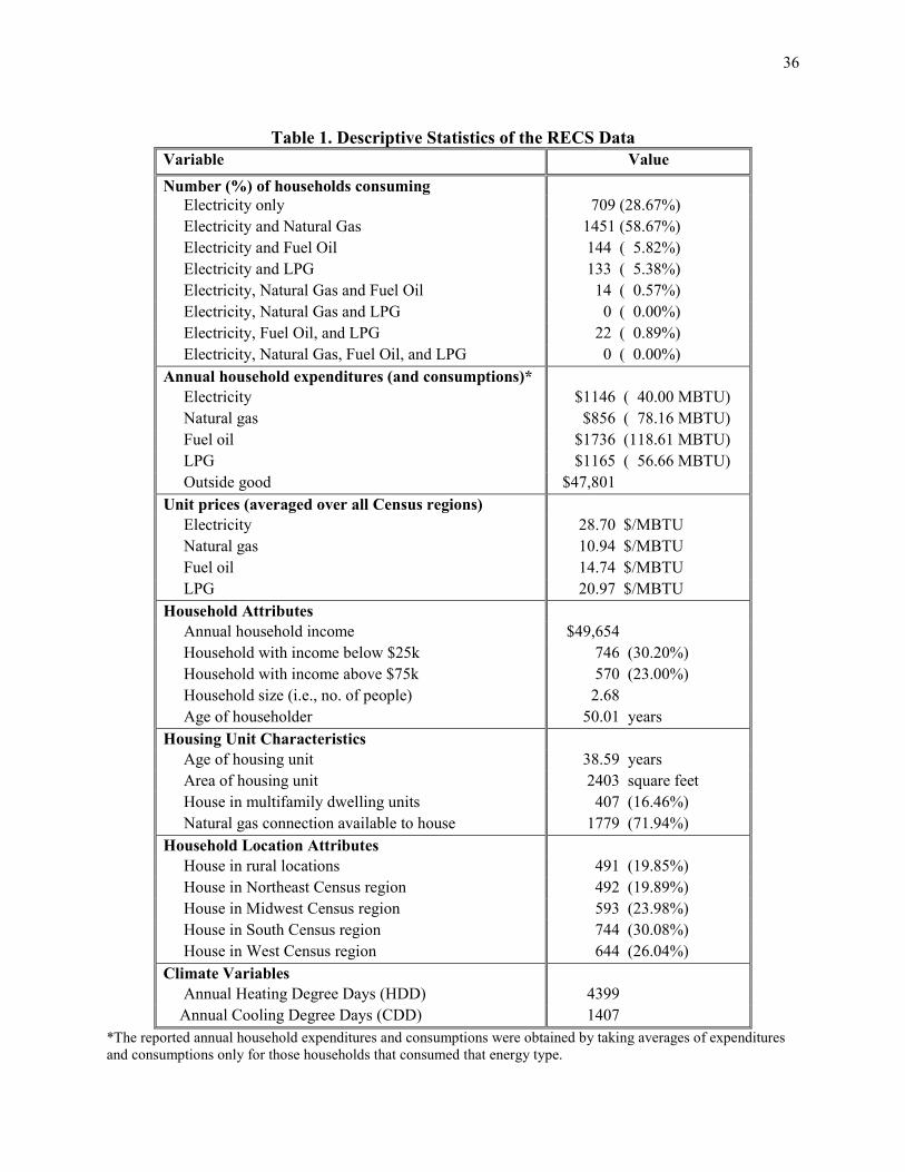
36

Table 1. Descriptive Statistics of the RECS Data

Variable Value

Number (%) of households consuming

Electricity only 709 (28.67%)

Electricity and Natural Gas 1451 (58.67%)

Electricity and Fuel Oil 144 ( 5.82%)

Electricity and LPG 133 ( 5.38%)

Electricity, Natural Gas and Fuel Oil 14 ( 0.57%)

Electricity, Natural Gas and LPG 0 ( 0.00%)

Electricity, Fuel Oil, and LPG 22 ( 0.89%)

Electricity, Natural Gas, Fuel Oil, and LPG 0 ( 0.00%)

Annual household expenditures (and consumptions)*

Electricity $1146 ( 40.00 MBTU)

Natural gas $856 ( 78.16 MBTU)

Fuel oil $1736 (118.61 MBTU)

LPG $1165 ( 56.66 MBTU)

Outside good $47,801

Unit prices (averaged over all Census regions)

Electricity 28.70 $/MBTU

Natural gas 10.94 $/MBTU

Fuel oil 14.74 $/MBTU

LPG 20.97 $/MBTU

Household Attributes

Annual household income $49,654

Household with income below $25k 746 (30.20%)

Household with income above $75k 570 (23.00%)

Household size (i.e., no. of people) 2.68

Age of householder 50.01 years

Housing Unit Characteristics

Age of housing unit 38.59 years

Area of housing unit 2403 square feet

House in multifamily dwelling units 407 (16.46%)

Natural gas connection available to house 1779 (71.94%)

Household Location Attributes

House in rural locations 491 (19.85%)

House in Northeast Census region 492 (19.89%)

House in Midwest Census region 593 (23.98%)

House in South Census region 744 (30.08%)

House in West Census region 644 (26.04%)

Climate Variables

Annual Heating Degree Days (HDD) 4399

Annual Cooling Degree Days (CDD) 1407

*The reported annual household expenditures and consumptions were obtained by taking averages of expenditures and consumptions only for those households that consumed that energy type.

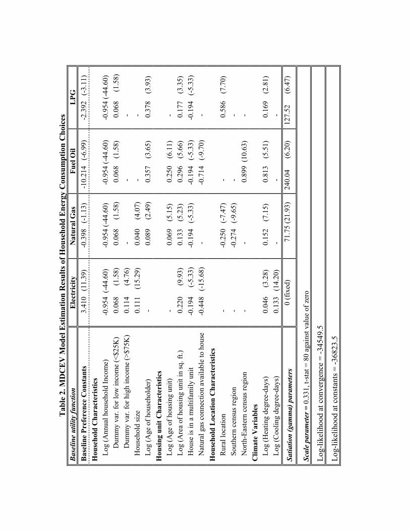
Table 2. MDCEV Model Estimation Results of Household Energy Consumption Choices

Baseline utility function

Electricity

Natural Gas

Fuel Oil

LPG

Baseline Preference Constants

3.410 (11.39)

-0.398 (-1.13)

-10.214 (-6.99)

-2.392 (-3.11)

Household Characteristics

Log (Annual household Income)

-0.954 (-44.60)

-0.954 (-44.60)

-0.954 (-44.60)

-0.954 (-44.60)

Dummy var. for low income (<$25K)

0.068 (1.58)

0.068 (1.58)

0.068 (1.58)

0.068 (1.58)

Dummy var. for high income (>$75K)

0.114 (4.76)

- -

-

Household size

0.111 (15.29)

0.040 (4.07)

- -

Log (Age of householder)

-

0.089 (2.49)

0.357 (3.65)

0.378 (3.93)

Housing unit Characteristics

Log (Age of housing unit)

- 0.069 (5.15)

0.250 (6.11)

-

Log (Area of housing unit in sq. ft.)

0.220 (9.93)

0.133 (5.23)

0.296 (5.66)

0.177 (3.35)

House is in a multifamily unit

-0.194 (-5.33)

-0.194 (-5.33)

-0.194 (-5.33)

-0.194 (-5.33)

Natural gas connection available to house

-0.448 (-15.68)

- -0.714 (-9.70)

-

Household Location Characteristics

Rural location

- -0.250 (-7.47)

- 0.586 (7.70)

Southern census region

- -0.274 (-9.65)

- -

North-Eastern census region

- -

0.899 (10.63)

-

Climate Variables

Log (Heating degree-days)

0.046 (3.28)

0.152 (7.15)

0.813 (5.51)

0.169 (2.81)

Log (Cooling degree-days)

0.133 (14.20)

- -

-

Satiation (gamma) parameters

0 (fixed)

71.75 (21.93)

240.04 (6.20)

127.52 (6.47)

Scale parameter = 0.331, t-stat = 80 against value of zero

Log-likelihood at convergence = -34549.5

Log-likelihood at constants = -36823.5

Table 3. Run Times of the Proposed and Existing Forecasting Algorithms

Proposed algorithm for γ-profile utility functions (Section 4.1)

Sample size

# Error draws

1000 households

2000 households

3000 households

4000 households

4382 households

100 sets

2.37 seconds

4.67 seconds

7.05 seconds

9.50 seconds

10.62 seconds

500 sets

11.49 seconds

23.01 seconds

34.71 seconds

45.92 seconds

50.77 seconds

Proposed algorithm for general utility functions (Section 4.2)

Sample size

# Error draws

1000 households

2000 households

3000 households

4000 households

4382 households

100 sets

10.36 seconds

20.86 seconds

31.06 seconds

41.63 seconds

45.71 seconds

500 sets

51.58 seconds

104.17 seconds

153.72 seconds

204.39 seconds

230.38 seconds

von Haefen et al. (2004) algorithm

Sample size

# Error draws

1000 households

2000 households

3000 households

4000 households

4382 households

100 sets

32.80 seconds

65.60 seconds

98.51 seconds

130.84 seconds

143.45 seconds

500 sets

163.56 seconds

326.70 seconds

491.42 seconds

651.66 seconds

717.69 seconds

Gradient-based constrained optimization routines of Gauss

Sample size

# Error draws

1000 households

2000 households

3000 households

4000 households

4382 households

1 set

3333 seconds

6237 seconds

9031 seconds

11876 seconds

12965 seconds

39

Table 4: Computational Performance of the Proposed Algorithms in Situations with Large Choice Sets

Budget 1

10

100

1000

10,000

100,000

Avg. no. of chosen alternatives 1.5 alts

10 alts

25 alts

49 alts

80 alts

115 alts

Computation Time in Seconds (for 1000 observations, with 50 different sets of error term draws)

Algorithms for γ-profile Utility Functions

Incremental enumeration (Section 4.1)

9.30 seconds

10.04 seconds

11.41 seconds

13.86 seconds

15.72 seconds

18.21 seconds

Bisection-based enumeration (Section 4.3.1)

12.10 seconds

12.03 seconds

12.12 seconds

12.30 seconds

12.56 seconds

12.90 seconds

Algorithms for General Utility Functions

(including α-profiles)

Incremental enumeration & bisection over λ-space (4.2)

12.84 seconds

16.50 seconds

25.46 seconds

44.50 seconds

75.72 seconds

111.70 seconds

Bisection over λ-space (4.3.2)

20.55 seconds

28.40 seconds

36.75 seconds

44.75 seconds

54.14 seconds

60.61 seconds

Bisection over consumption space (von Haefen et al., 2004)

22.70 seconds

31.66 seconds

38.11 seconds

45.22 seconds

54.39 seconds

60.86 seconds

Table 5. Predicted and Observed Energy Consumption Patterns in the Base Case

Sample Predictions

Sample Observations

Population Predictions

Population Observations

Average

annual

household

expenditure

($)

Average

annual

Household

consumption

(Million BTU)

Average

annual

household

expenditure

($)

Average annual

household

consumption

(Million BTU)

Total annual

expenditure

in all houses

in the U.S.

(Billion $)

Total Annual

consumption

in all houses

in the U.S.

(Trillion BTU)

Total Annual

Expenditure

in all houses

in the U.S.

(Billion $)

Total Annual

consumption

in all houses

in the U.S.

(Trillion BTU)

Outside good

45766 (37.2)

--

45805

--

5235.24 (4.0)

--

5239.99

--

Electricity

1100 (17.2)

38 (0.6)

1116

39

123.16 (2.0)

4314 ( 68.3)

124.66

4349

Natural Gas

548 (21.4)

50 (2.0)

487

44

59.66 (2.4)

5515 (217.8)

52.38

4793

Fuel Oil

157 (21.2)

11 (1.4)

149

10

13.62 (1.9)

925 (127.3)

12.75

865

LPG

84 (10.7)

4 (0.5)

98

5

9.11 (1.1)

436 ( 55.3)

11.00

524

40

Table 6. Predicted Energy Consumption/Expenditure Changes in Response to Climate Change Scenarios

450o Fahrenheit Increase in Annual Cooling Degree Days

450o Fahrenheit Increase in Annual Heating Degree Days

Predicted changes in energy

expenditures (Billion $)

Predicted changes in energy

consumption (Trillion BTU)

Predicted changes in energy

expenditures (Billion $)

Predicted changes in energy

consumption (Trillion BTU)

Average (Standard error)

Average (Standard error)

Average (Standard error)

Average (Standard error)

Outside good -5.281 (0.454)

--

-5.104 (0.591)

--

Electricity

5.581 (0.478)

189.78 (16.31)

0.900 (0.267)

32.23 ( 9.42)

Natural Gas

-0.169 (0.016)

-15.72 ( 1.44)

2.079 (0.213)

191.48 (19.63)

Fuel Oil

-0.074 (0.010)

-5.03 ( 0.70)

1.712 (0.371)

116.06 (25.16)

LPG

-0.057 (0.009)

-2.70 ( 0.41)

0.413 (0.134)

18.92 ( 6.25)

Table 7. Predicted Energy Consumption/Expenditure Changes in Scenarios Associated with House Area Sizes in the U.S.

House Area Increased by 10%

House Area Decreased by 10%

Predicted changes in energy

expenditures (Billion $)

Predicted changes in energy

consumption (Trillion BTU)

Predicted changes in energy

expenditures (Billion $)

Predicted changes in energy

consumption (Trillion BTU)

Average (Standard error)

Average (Standard error)

Average (Standard error)

Average (Standard error)

Outside good -4.741 (0.631)

--

5.117 (0.670)

--

Electricity

2.405 (0.284)

84.39 ( 9.97)

-2.609 (0.303)

-91.55 (10.63)

Natural Gas

1.204 (0.271)

110.93 (24.97)

-1.313 (0.292)

-120.97 (26.84)

Fuel Oil

0.797 (0.162)

54.10 (11.02)

-0.836 (0.165)

-56.77 (11.21)

LPG

0.335 (0.117)

15.89 ( 5.55)

-0.358 (0.121)

-17.00 ( 5.77)