Computational topology. - Penn Mathdlotko/IAS_dlotko.pdf · Computational topology. Paweł Dłotko...
121
Computational topology. Pawel Dlotko 13/03/2013 IAS.
Transcript of Computational topology. - Penn Mathdlotko/IAS_dlotko.pdf · Computational topology. Paweł Dłotko...

Computational topology.
Paweł Dłotko
13/03/2013 IAS.

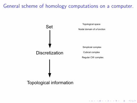
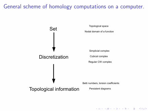
General scheme of homology computations on a computer.
Set

General scheme of homology computations on a computer.
SetTopological space

General scheme of homology computations on a computer.
SetTopological space
Nodal domain of a function

General scheme of homology computations on a computer.
SetTopological space
Nodal domain of a function
Discretization

General scheme of homology computations on a computer.
SetTopological space
Nodal domain of a function
Discretization
Simplicial complex

General scheme of homology computations on a computer.
SetTopological space
Nodal domain of a function
Discretization
Simplicial complex
Cubical complex

General scheme of homology computations on a computer.
SetTopological space
Nodal domain of a function
Discretization
Simplicial complex
Cubical complex
Regular CW complex
General scheme of homology computations on a computer.
SetTopological space
Nodal domain of a function
Discretization
Topological information
Simplicial complex
Cubical complex
Regular CW complex

General scheme of homology computations on a computer.
SetTopological space
Nodal domain of a function
Discretization
Topological information
Simplicial complex
Cubical complex
Regular CW complex
Betti numbers, torsion coefficients
General scheme of homology computations on a computer.
SetTopological space
Nodal domain of a function
Discretization
Topological information
Simplicial complex
Cubical complex
Regular CW complex
Betti numbers, torsion coefficients
Persistent diagrams

General scheme of homology computations on a computer.
SetTopological space
Nodal domain of a function
Discretization
Topological information
Simplicial complex
Cubical complex
Regular CW complex
Betti numbers, torsion coefficients
Persistent diagrams
(co)homolgy generators

General scheme of homology computations on a computer.
SetTopological space
Nodal domain of a function
Discretization
Topological information
Simplicial complex
Cubical complex
Regular CW complex
Betti numbers, torsion coefficients
Persistent diagrams
(co)homolgy generators

Representation of spaces.
1. (Abstract) simplicial complex.
2. Cubical complex.
3. Regular CW-complex.
4. Chain complex.
5. For reduction methods we need to iterate among neighboringcells fast.

Abstract simplicial complex.
class Simplex{//..vector<Simplex*> faces;vector<Simplex*> cofaces;double filtrationLevel;int id;//some extra information};
class AbstractSimplicialComplex{//..vector< vector<Simplex*> > elements;//graded vector of simplices;};

Representation in RAM vs Mathematics.
1
2
3
4
RAM Mathematics
1
2
3
412
13
23
24123

Regular vs not regular grids.
1. Simplicial complexes do not have regular structure.
2. The size of data structure to store simplex ∼ number of itsfaces times 32 bits.
3. Regular grids allows us to decrease drastically amount ofmemory needed to store the structure.
4. Possible to get neighbors of a given cell from the structure ofa grid.
5. Cubical grids with cubes having equal sizes forms regular grids.
6. 1 bit of information per cube suffices (for complex) or 1 realnumber (8 bytes = 64 bits) for complex with filtration.

The Bitmap (basic version).
3
3
bool* bitmap; //!! Be careful!char* bitmap; //This is the right way in C++.

Regular vs not regular grids.
1. One can build bitmap in any dimension, 2d is just to presentthe idea.
2. All the bitmaps caches very well.
3. Only top dimensional cubes are represented.
4. Elementary reductions or acyclic subspace method can beused.
5. After reduction, the chain complex of the remaining set iscreated.
6. There are bitmaps in which all the cells of complex arerepresented.

The Bitmap.

Rectangular / Regular CW-complex.
1. Obtained as topologically faithful representation of a nodaldomain of a function.
2. They are represented in the same way as simplicial complexes(vectors of pointers).
3. In case of nodal domains of random trig. polynomials this is abetter representation then a bitmap of uniform size cubes.

Sparse matrix representation (for chain complexes overZ2).
1. General chain complex is stored as a sparse matrix.
2. They are usually represented as a vector of lists.
3. For easy access to coboundary it can be stored by using thesame structure.
1 2 3 4 5 6
7
45
549
12 3
7
7
65
12

Other representations.
1. Rectangular CW-complexes (quad-trees, oct-trees).
2. Point clouds - Rips complexes via Rips graph.
3. Voronoi diagrams.
4. Some representation for 2-dimensional simplicial complexesused in computer graphics.

What is the best representation for your purposes?
1. Everything here is just my intuition.
2. No universal data structure – the best one depends on yourdata and problem to solve.
3. For regular cubical set, bitmap representation is natural.
4. If the cubes have different sizes, representation of rectangularset may be better.
5. For simplicial complex if access to (co)boundary is needed –try pointer representation.
6. Almost always pays off to use sparse matrix data structureunless your data are very small.
Reduction methods.
1. Reduction methods were developed as heuristic to enablehomology computations for big data.
2. Elementary reduction aka. free face collapsing.
3. Coreductions.
4. Acyclic subspace method.
5. Algebraic reductions (KMS).
6. I will give some intuitive demonstration why they work basedon Discrete Morse Theory.

Procedure 1 Elementary reduction.Input: vector of cell complex;
queue T;for every a in complex doif a has unique coboundary element then
T.enqueue( a );while T is not empty do
cell a = T.dequeue();if a has unique element b in coboundary then
remove a and b from complex;for every c face of b such that c!=a doif c has unique coboundary element then
T.enqueue(c);for every c face of a doif c has unique coboundary element then
T.enqueue(c);

Elementary Reductions.

Elementary reductions
Procedure 2 Elementary reduction.Input: vector of cell complex;
queue T;
for every a in complex doif a has unique coboundary element thenT.enqueue( a );
while T is not empty docell a = T.dequeue();if a has unique element b in coboundary then
remove a and b from complex;for every c face of b such that c!=a doif c has unique coboundary element then
T.enqueue(c);for every c face of a doif c has unique coboundary element then
T.enqueue(c);

Elementary Reductions.

Procedure 3 Elementary reduction.Input: vector of cell complex;
queue T;for every a in complex doif a has unique coboundary element then
T.enqueue( a );while T is not empty do
cell a = T.dequeue();
if a has unique element b in coboundary thenremove a and b from complex;for every c face of b such that c!=a doif c has unique coboundary element then
T.enqueue(c);for every c face of a doif c has unique coboundary element then
T.enqueue(c);

Elementary Reductions.
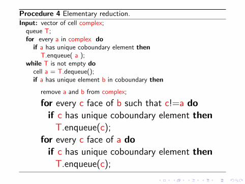
Procedure 4 Elementary reduction.Input: vector of cell complex;
queue T;for every a in complex doif a has unique coboundary element then
T.enqueue( a );while T is not empty do
cell a = T.dequeue();if a has unique element b in coboundary then
remove a and b from complex;
for every c face of b such that c!=a doif c has unique coboundary element then
T.enqueue(c);for every c face of a doif c has unique coboundary element then
T.enqueue(c);

Elementary Reductions.

Elementary Reductions.

Elementary Reductions.

Elementary Reductions.

Elementary Reductions.

Elementary Reductions.

Elementary Reductions.

Elementary Reductions.

Elementary Reductions.
1. Introduced by J. H. C. Whitehead.
2. Homotopy equivalence.
3. Morse paths do not start at any critical cell (they go fromboundary to interior).
4. Morse complex is identical to the initial complex minusreduced cells.

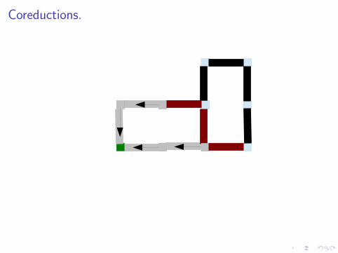
Coreductions.
Procedure 5 Coreduction.Input: vector of cell complex;
queue T;Remove a single vertex v from complex;for Every c in coboundary of v do
T.enqueue(c);while T is not empty do
c = T.dequeue();if c has unique element b in boundary then
remove c and b from the complex;for every element e in coboundary of b doif e has unique element in boundary then
T.enqueue(e);for every element e in cobounday of c doif e has unique element in boundary then
T.enqueue(e);

Coreductions.

Coreductions.
Procedure 6 Coreduction.Input: vector of cell complex;
queue T;Remove a single vertex v from complex;for Every c in coboundary of v do
T.enqueue(c);while T is not empty do
c = T.dequeue();if c has unique element b in boundary then
remove c and b from the complex;for every element e in coboundary of b doif e has unique element in boundary then
T.enqueue(e);for every element e in cobounday of c doif e has unique element in boundary then
T.enqueue(e);

Coreductions.

Coreductions.
Procedure 7 Coreduction.Input: vector of cell complex;
queue T;
Remove a single vertex v from complex;
for Every c in coboundary of v doT.enqueue(c);while T is not empty do
c = T.dequeue();if c has unique element b in boundary then
remove c and b from the complex;for every element e in coboundary of b doif e has unique element in boundary then
T.enqueue(e);for every element e in cobounday of c doif e has unique element in boundary then
T.enqueue(e);

Coreductions.

Coreductions.
Procedure 8 Coreduction.Input: vector of cell complex;
queue T;Remove a single vertex v from complex;for Every c in coboundary of v do
T.enqueue(c);
while T is not empty doc = T.dequeue();if c has unique element b in boundary thenremove c and b from the complex;for every element e in coboundary of b doif e has unique element in boundary then
T.enqueue(e);for every element e in cobounday of c doif e has unique element in boundary then
T.enqueue(e);

Coreductions.

Coreductions.
Procedure 9 Coreduction.Input: vector of cell complex;
queue T;Remove a single vertex v from complex;for Every c in coboundary of v do
T.enqueue(c);while T is not empty do
c = T.dequeue();if c has unique element b in boundary then
remove c and b from the complex;
for every element e in coboundary of b doif e has unique element in boundarythenT.enqueue(e);
for every element e in cobounday of c doif e has unique element in boundarythenT.enqueue(e);

Coreductions.

Coreductions.
Procedure 10 Coreduction.Input: vector of cell complex;
queue T;Remove a single vertex v from complex;for Every c in coboundary of v do
T.enqueue(c);
while T is not empty doc = T.dequeue();if c has unique element b in boundary thenremove c and b from the complex;for every element e in coboundary of b doif e has unique element in boundary then
T.enqueue(e);for every element e in cobounday of c doif e has unique element in boundary then
T.enqueue(e);

Coreductions.
Coreductions.

Coreductions.

Coreductions.

Coreductions.

Coreductions.

Coreductions.

Coreductions of torus.
1 1
11
7
6
5
432
5
6
7
2 3 4

Coreductions of torus.
1 1
11
7
6
5
432
5
6
7
2 3 4

Coreductions of torus.
1 1
11
7
6
5
432
5
6
7
2 3 4

Coreductions of torus.
1 1
11
7
6
5
432
5
6
7
2 3 4

Coreductions of torus.
1 1
11
7
6
5
432
5
6
7
2 3 4

Coreductions of torus.
1 1
11
7
6
5
432
5
6
7
2 3 4

Coreductions of torus.
1 1
11
7
6
5
432
5
6
7
2 3 4

Coreduction.
1. Introduced by Mrozek and Batko.
2. Easy to explain then in language of Discrete Morse Theory.
3. Unique critical (green) point in dimension 0.
4. Gradient field contract everything towards it.
5. Every critical edge has empty boundary.
6. Every gradient path starting at boundary of higher dimensioncritical cell do not end in any lower dimensional critical cell.
7. Multi-point coreduction (used in parallel programs).

Multi-point coreduction.

Multi-point coreduction.

Multi-point coreduction.

Multi-point coreduction.

Acyclic subspace.
1. Introduced by Mrozek, Pilarczyk and Zelazna.
2. A ⊂ K such that Hn(A) are trivial (acyclic subcomplex).
3. Hn(K ) ' Hn(K ,A) for n > 0 and H0(K ) ' H0(K ,A)⊕ Z(Mayer-Vietoris).
4. Hn(K ,A) ' Hn(K \ A) (Mrozek, Batko).
5. Greedy strategy to build as large A as possible.

Acyclic subcomplex.

Acyclic subcomplex.

Acyclic subcomplex.

Acyclic subcomplex.

Acyclic subcomplex.

Acyclic subcomplex.

Acyclic subcomplex.

Acyclic subcomplex.

Acyclic subspace.
1. This algorithm operates only on top dimensional cells.
2. Can be applied to the basic version of a bitmap.
3. Test needed to determine if an element can be added toacyclic subcomplex.
4. Full test - homology computations, tabulated configurations(2/3d cubes, 2/3/4d simplices).
5. Partial tests – higher dimensions.
6. Coreduction algorithm is also kind of acyclic subspacealgorithm.

Retrieving of generators.
1. In some applications Betti numbers and torsions coefficientare not sufficient.
2. Sometimes representatives of generators are needed.
3. Example of such a application – electromagnetic modeling (wewill consider case of Ampere’s law).
4. Local Ampere’s law: For every face f ,〈EM, ∂f 〉 = 〈Current, f 〉.

Ampere’s law.
Conductor

Ampere’s law.
Conductor

Retrieving generator.

Retrieving generator.

Retrieving generator.

Retrieving generator.

Retrieving generator.

Retrieving generator.

Retrieving generator.
Retrieving of generators.
1. Restoring generator takes O(n) time per generator.
2. The constant is considerable.
3. It pays off to use so called shaving as a first reduction.
4. Shaving is a reduction such that there is no need to restoregenerators...
5. i.e. embeddings of generators in reduced complex aregenerators in initial complex.
6. Elementary reductions is a shaving for homology.
7. Acyclic subspace and coreductions are shaving for cohomology.
8. For EM computations shaving gives about order of magnitudespeed up in computations.

Shaving for homology.

Shaving for cohomology.

KMS - algebraic reductions.
1. Algebraic reduction – bases on making a single Morse pairingat a time:
AB
c A
2. ∂A = ∂A− 〈∂B, c〉−1〈∂A, c〉∂B provided 〈∂B, c〉 is invertible.
3. Such a reduction is applied iteratively.

What to do when the reductions are done?
1. Reductions are heuristics.
2. They works very well in the applications we are considering(dynamical systems, engineering, material analysis).
3. They give a Betti numbers and generators in planar and2-manifold case (no SNF needed).
4. For some algebraic complexes they works much worst.
5. To obtain integer homology at the end SNF algorithm isneeded.
6. For field homology and persistence one can use also iteratedMorse approach.

Homology of nodal domains of continuous functions.
1. There are rigorous partial algorithms to compute homology ofnodal domains of a function.
2. A function u : R2 → R is given as a computer program(formula, numerical method) ...
3. such that it can be evaluated with interval arithmetic.
4. With this information topologically faithful representation ofnodal domains can be obtained.

Initial discretization of the domain.

Initial discretization of the domain.

Validation algorithm.
1. For every rectangle R...
2. make sure that in each corner x ∈ R the value of u(x) 6= 0. Ifit is, then failure.
3. If all the signs are the same, then compute [u(R), u(R)]. If itcontain zero, then subdivide. Otherwise OK.
4. If all but one signs are the same, then if either ux(R) or uy (R)contain zero, then subdivide. Else OK.
5. If two corners (upper/lower) are positive and other two(lower/upper) are negative then if:5.1 u on lower and upper edge does not contain zero and5.2 ux(R) does contain zero
then OK, else subdivide. The same in case of left/right.

Nodal domains of random trigonometric polynomial.

How to compute homology of non-regular cubical grid?
1. Subdivision to cubical complex.
2. Homology of Cech complex.
3. Computational homology theory for regular CW-complexes.
4. The key point is to obtain incidence coefficients – Massey’sequations.

Massey’s equations.

Massey’s equations.
-1
-1 +1
+1
+1
-1
-1 +1-1
+1
+1
-1

Massey’s equations.
-1
-1 +1
+1
+1
-1
-1 +1-1
+1
+1
-1
+1

Massey’s equations.
-1
-1 +1
+1
+1
-1
-1 +1-1
+1
+1
-1
+1
-1

Massey’s equations.
-1
-1 +1
+1
+1
-1
-1 +1-1
+1
+1
-1
+1
-1
+1

Massey’s equations.
-1
-1 +1
+1
+1
-1
-1 +1-1
+1
+1
-1
+1
-1
+1
+1

Massey’s equations.
-1
-1 +1
+1
+1
-1
-1 +1-1
+1
+1
-1
+1
-1
+1
+1-1

Massey’s equations.
-1
-1 +1
+1
+1
-1
-1 +1-1
+1
+1
-1
+1
-1
+1
+1
-1
-1

Massey’s equations.
-1
-1 +1
+1
+1
-1
-1 +1-1
+1
+1
-1
+1
-1
+1
+1
-1
-1

Once we have incidence coefficients.
1. Any presented reduction method can be used.
2. In case of random trigonometric polynomials the memory usedby the pointer structure is order(s) of magnitude lower thanby corresponding uniform cubical grid.
3. Also, computational times are ∼ two orders of magnitudebetter.
4. But this is what we see in practice for random trig.polynomials.
5. Intuition - if the ’shape’ of nodal domain is not verycomplicated, then the pointer representation is superior.
6. If it become ver complicated / chaotic / fractal, then regularcubical grid may be better.

Delfinado-Edelsbrunner incremental algorithm.
1. It is a first algorithm to compute homology different fromstandard SNF algorithm.
2. It works for sub-triangulations of S3.
3. Bases on Alexander duality – X - sub-triangulation of S3,Y = S3 \ X .
4. Hq(Y ) ' H2−q(X ). Since there are no torsions in R3 =⇒βq(Y ) = β2−q(X ).
5. 2−cycles in X are 1-1 to connected components in Y .

Delfinado-Edelsbrunner incremental algorithm.
1. σ1, σ2, . . . , σn triangulation of S3 such that every prefix is asimplicial complex.
2. Xi = {σ1, σ2, . . . , σi}.3. Suppose σi+1 of dimension d is added to Xi . Then eitherβd(Xi+1) = βd(Xi ) + 1 or βd−1(Xi+1) = βd−1(Xi )− 1.
4. If σi+1 is a vertex, then always β0(Xi+1) = β0(Xi ) + 1.
5. If σi+1 is edge or triangle, then we should determine if itcloses a cycle.
6. If it does, βdim(σi+1) increase, if not βdim(σi+1)−1 decrease.

Detecting 1-cycles.
1. Analyzing connected components of 1-skeleton.

Detecting 2-cycles.
1. Analyzing connected components of complex complement.

Delfinado-Edelsbrunner incremental algorithm.
Procedure 11 Incremental Algorithm (non-optimal version!).Input: σ1, . . . , σn filtration of S3;β0 = β1 = β2 = β3 = 0;for i = 1 to n doif σi is a vertex thenβ0 + +;if σi is an edge thenif σi close a cycle in Xi−1 thenβ1 + +;elseβ0 −−;if σi is a triangle thenif σi close a cycle in S3 \ Xi thenβ1 −−;elseβ2 + +;
if i = n thenβ3 = 1;

Bibliography.
1. Data structures:1.1 T. Kaczynski, K. Mischaikow, and M. Mrozek, ”Computational
Homology” (book).1.2 H. Edelsbrunner and J. Harer, ”Computational Topology”
(book).1.3 P.D., T. Kaczynski, M. Mrozek, Th. Wanner, ”Coreduction
Homology Algorithm for Regular CW-Complexes”.1.4 Chomp – Computational Homology Project (soft).1.5 CAPD – Coputer Assisted Proofs in Dynamic (soft).1.6 Soft for persistence (ancient mythology) – Dionysus (D.
Morozov), Perseus (V. Nanda),1.7 Soft for persistence (rest) – (J)Plex (Stanford), Homology
with a Twist (IST Austria).

Bibliography.
1. Reduction methods:1.1 T. Kaczynski, K. Mischaikow, and M. Mrozek, ”Computational
Homology” (book).1.2 R. Forman, ”A user’s guide to discrete Morse theory”.1.3 T. Kaczynski M. Mrozek and M. Slusarek, ”Homology
Computation by Reduction of Chain Complexes”.1.4 M. Mrozek, P. Pilarczyk, N. Zelazna, ”Homology Algorithm
Based on Acyclic Subspace”.1.5 M. Mrozek, B. Batko, Coreduction Homology Algorithm.1.6 P. Brendel, P. D., M. Mrozek, N. Zelazna, ”Homology
Computations via Acyclic Subspace”.

Bibliography.
1. Cohomology computations:1.1 P. D., R. Specogna ”Efficient cohomology computation for
electromagnetic modeling”.
2. Homology of nodal domain:2.1 S. Day, W. Kalies, Th. Wanner ,”Verified homology
computations for nodal domains”.2.2 P.D., T. Kaczynski, M. Mrozek, Th. Wanner, ”Coreduction
Homology Algorithm for Regular CW-Complexes”.2.3 G. Cochran, Th. Wanner, P.D., ”A randomized subdivision
algorithm for determining the topology of nodal sets”.2.4 W. S. Massey, ”A Basic Course in Algebraic Topology” (book).
3. Delfinado-Edelsbrunner (Incremental Algorithm):3.1 C. Delfinado, H. Edelsbrunner, ”An incremental algorithm for
Betti numbers of simplicial complexes”.3.2 H. Edelsbrunner and J. Harer, ”Computational Topology”
(book).

Thank you for your time!
Pawel DlotkoUniversity of Pennsylvania
[email protected] dlotko @ skype
pdlotko @ gmail