Statistical Methods for Analyzing Ordered Gene Expression Microarray Data

Computational Methods for Analyzing andModeling Gene Regulation Dynamics
Jason Ernst
August 2008 CMU-ML-08-110

Computational Methods for Analyzing andModeling Gene Regulation Dynamics
Jason Ernst
August 2008CMU-ML-08-110
School of Computer ScienceMachine Learning Department
Carnegie Mellon UniversityPittsburgh, PA
Thesis Committee:Ziv Bar-Joseph (Chair)
Zoubin GhahramaniEric P. Xing
Naftali Kaminski, University of PittsburghZoltan N. Oltvai, University of Pittsburgh
Submitted in partial fulfillment of the requirementsfor the Degree of Doctor of Philosophy
Copyright c©2008 Jason Ernst
This research was sponsored by the National Institute of Health under grant no.HHSN2666200500018C and a Siebel Scholarship.The views and conclusions contained in this document are those of the author and should not be interpreted as representing the officialpolicies, either expressed or implied, of any sponsoring institution, the U.S. government or any other entity.

Keywords: Dynamics, Gene Expression, Gene Regulation, Microarray, Regulatory Networks,
Time course, Time series, Transcription, Transcription Factor
Abstract
Gene regulation is a central biological process whose disruption can lead to many diseases. This
process is largely controlled by a dynamic network of transcription factors interacting with specific
genes to control their expression. Time series microarray gene expression experiments have be-
come a widely used technique to study the dynamics of this process. This thesis introduces new
computational methods designed to better utilize data from these experiments and to integrate this
data with static transcription factor-gene interaction data to analyze and model the dynamics of gene
regulation. The first method, STEM (Short Time-series Expression Miner), is a clustering algorithm
and software specifically designed for short time series expression experiments, which represent the
substantial majority of experiments in this domain. The second method, DREM (Dynamic Regu-
latory Events Miner), integrates transcription factor-gene interactions with time series expression
data to model regulatory networks while taking into account their dynamic nature. The method uses
an Input-Output Hidden Markov Model to identify bifurcation points in the time series expression
data. While the method can be readily applied to some species, the coverage of experimentally
determined transcription factor-gene interactions in most species is limited. To address this we
introduce two methods to improve the computational predictions of these interactions. The first
of these methods, SEREND (SEmi-supervised REgulatory Network Discoverer), motivated by the
species E. coli is a semi-supervised learning method that uses verified transcription factor-gene in-
teractions, DNA sequence binding motifs, and gene expression data to predict new interactions. We
also present a method motivated by human genomic data, that combines motif information with a
probabilistic prior on transcription factor binding at each location in the organism’s genome, which
it infers based on a diverse set of genomic properties. We applied these methods to yeast, E. coli,
and human cells. Our methods successfully predicted interactions and pathways, many of which
have been experimentally validated. Our results indicate that by explicitly addressing the temporal
nature of regulatory networks we can obtain accurate models of dynamic interaction networks in
the cell.
i


Acknowledgements
First, I would like to acknowledge my advisor and mentor, Ziv Bar-Joseph. Ziv started me in the
field of computational biology, and along the path of research that has led to this thesis. While going
down this path he has constantly been there to provide me advice, guidance, and support.
In addition to my advisor, I am privileged to have on my thesis committee: Zoubin Ghahramani,
Naftali Kaminski, Zoltan Oltvai, and Eric Xing. This committee has provided me access to tremen-
dous breadth and depth of expertise in machine learning and biology. This thesis has benefited from
their insightful comments, ideas, and suggestions. I was also fortunate to have spent part of the
Summer of 2004 in Naftali’s lab. During that time I had the opportunity to experience first-hand
the ‘wet’ side of biology, and the discussions I had then with members of his lab largely provided
me the impetus to develop STEM into software that would become broadly used by experimental
biologists.
Chapters 2, 3, and 4 of this thesis are based on papers co-authored by subsets of Gabor Balazsi,
Ziv Bar-Joseph, Qasim Beg, Chris Harbison, Krin Kay, Jerry Nau, Zoltan Oltvai, Itamar Simon,
and Oded Vainas. In particular I want to acknowledge that Oded working in Itamar’s lab conducted
the biological experiments to validate computational predictions in Chapter 3, and Qasim and Krin
working in Zoltan’s lab generated the time series microarray data used as part of the experimental
validation in Chapter 4.
I have many other people to acknowledge and thank. A general acknowledgement goes to
everyone with whom I have had discussions about the research in this thesis. Richard Steinman
for our collaboration, which while not presented in this thesis, I still consider to be an important
iii

iv Acknowledgements
experience during my graduate studies. Current and former members of the systems biology group:
Anthony Gitter, Akshay Goel, Henry Lin, Yong Lu, Dima Patek, Peter Pong, Yanjun Qi, Yanxin
Shi, and Guy Zinman for their comments, help, and discussions. The users of STEM and DREM
for the useful feedback and encouragement they have provided to me. All the students, faculty, and
staff of the Machine Learning Department for making it such a stimulating environment to be a
graduate student, with a special mention going to Diane Stidle for keeping the department running
so smoothly.
Finally, I would like to acknowledge my parents for their support.

Table of Contents
1 Introduction 11.1 Transcription Factor-Gene Regulation . . . . . . . . . . . . . . . . . . . . . . . . 2
1.2 Microarray Background . . . . . . . . . . . . . . . . . . . . . . . . . . . . . . . . 2
1.3 Time Series Microarray Experiments . . . . . . . . . . . . . . . . . . . . . . . . . 4
1.4 Inferring the Location of Transcription Factor Binding . . . . . . . . . . . . . . . 7
1.4.1 Motif Scanning . . . . . . . . . . . . . . . . . . . . . . . . . . . . . . . . 7
1.4.2 High-throughput Experimental Methods . . . . . . . . . . . . . . . . . . . 9
1.5 Static Methods for Analysis of Gene Regulation . . . . . . . . . . . . . . . . . . . 11
1.6 Overview of Thesis . . . . . . . . . . . . . . . . . . . . . . . . . . . . . . . . . . 12
2 Clustering Short Time Series Gene Expression Data 152.1 Introduction . . . . . . . . . . . . . . . . . . . . . . . . . . . . . . . . . . . . . . 15
2.1.1 Related work . . . . . . . . . . . . . . . . . . . . . . . . . . . . . . . . . 16
2.2 Identifying significant expression patterns . . . . . . . . . . . . . . . . . . . . . . 18
2.2.1 Selecting model profiles . . . . . . . . . . . . . . . . . . . . . . . . . . . 18
2.2.2 Identifying significant model profiles . . . . . . . . . . . . . . . . . . . . 23
2.2.3 Correlation Coefficient . . . . . . . . . . . . . . . . . . . . . . . . . . . . 25
2.2.4 Grouping Significant Profiles . . . . . . . . . . . . . . . . . . . . . . . . . 27
2.3 Results . . . . . . . . . . . . . . . . . . . . . . . . . . . . . . . . . . . . . . . . . 28
2.4 Software Implementation - Short Time Series Expression Miner . . . . . . . . . . 37
2.5 Discussion . . . . . . . . . . . . . . . . . . . . . . . . . . . . . . . . . . . . . . . 40
3 Reconstructing Dynamic Regulatory Maps 433.1 Introduction . . . . . . . . . . . . . . . . . . . . . . . . . . . . . . . . . . . . . . 43
3.2 Method - Dynamic Regulatory Events Miner (DREM) . . . . . . . . . . . . . . . 46
3.2.1 Probabilistic Model . . . . . . . . . . . . . . . . . . . . . . . . . . . . . . 48
3.2.2 Parameter Learning . . . . . . . . . . . . . . . . . . . . . . . . . . . . . . 51
v

vi TABLE OF CONTENTS
3.2.3 Model Selection . . . . . . . . . . . . . . . . . . . . . . . . . . . . . . . 52
3.2.4 Transcription Factor Scoring . . . . . . . . . . . . . . . . . . . . . . . . . 56
3.3 Results . . . . . . . . . . . . . . . . . . . . . . . . . . . . . . . . . . . . . . . . . 57
3.3.1 A temporal map for amino-acid starvation response . . . . . . . . . . . . . 57
3.3.2 Extending condition-specific dynamic maps using general binding data . . 60
3.3.3 Validating interactions and mechanistic predictions . . . . . . . . . . . . . 62
3.3.4 Temporal maps for the regulation of stress response in yeast . . . . . . . . 62
3.3.5 Determining the activation time of regulators . . . . . . . . . . . . . . . . 70
3.3.6 Verifying the advantage of integrating time series expression and ChIP-chipdata . . . . . . . . . . . . . . . . . . . . . . . . . . . . . . . . . . . . . . 76
3.3.7 Modeling Convergence of Paths from a Split . . . . . . . . . . . . . . . . 80
3.3.8 Interpolation . . . . . . . . . . . . . . . . . . . . . . . . . . . . . . . . . 81
3.4 Software Implementation . . . . . . . . . . . . . . . . . . . . . . . . . . . . . . . 82
3.5 Discussion . . . . . . . . . . . . . . . . . . . . . . . . . . . . . . . . . . . . . . . 83
4 A Semi-Supervised Method for Predicting Transcription Factor-Gene Interactions inEscherichia coli 874.1 Introduction . . . . . . . . . . . . . . . . . . . . . . . . . . . . . . . . . . . . . . 87
4.2 SEREND Method: Ranking Target Predictions for a Transcription Factor . . . . . 90
4.3 Results . . . . . . . . . . . . . . . . . . . . . . . . . . . . . . . . . . . . . . . . . 98
4.3.1 Evaluation of Predictions: Comparison with ChIP-chip Data . . . . . . . . 100
4.3.2 Biological Functional Analysis of Predicted Targets of Global Regulators . 105
4.3.3 Application to Aerobic-Anaerobic Shift . . . . . . . . . . . . . . . . . . . 106
4.4 Discussion . . . . . . . . . . . . . . . . . . . . . . . . . . . . . . . . . . . . . . . 113
5 Integrating Multiple Evidence Sources to Predict Transcription Factor Binding acrossthe Human Genome 1175.1 Introduction . . . . . . . . . . . . . . . . . . . . . . . . . . . . . . . . . . . . . . 117
5.2 An Informative Empirical Prior on Transcription Factor Binding . . . . . . . . . . 119
5.2.1 Method to Learn the Empirical Prior . . . . . . . . . . . . . . . . . . . . . 119
5.2.2 Results Using just the Prior . . . . . . . . . . . . . . . . . . . . . . . . . 126
5.3 Combining the Prior with Motif Information . . . . . . . . . . . . . . . . . . . . . 132
5.3.1 Method for Combining the Prior with Motif Evidence . . . . . . . . . . . 132
5.3.2 Results for Combining the Prior with Motif Information . . . . . . . . . . 134
5.4 Discussion . . . . . . . . . . . . . . . . . . . . . . . . . . . . . . . . . . . . . . . 138

TABLE OF CONTENTS vii
6 Conclusions and Future Work 1436.1 Conclusions . . . . . . . . . . . . . . . . . . . . . . . . . . . . . . . . . . . . . . 1436.2 Future Work . . . . . . . . . . . . . . . . . . . . . . . . . . . . . . . . . . . . . . 146


Chapter 1
Introduction
Transcriptional gene regulation is a central cellular process. During transcription, the DNA of a
gene is used as a template from which messenger RNA (mRNA) is produced. The mRNA is then
later translated into proteins, the workhorse molecules of the cell. The regulation of transcription
is a dynamic process where in response to stimuli specific type of proteins, called transcription
factors, dynamically activate or repress the transcription of genes. Problems with transcriptional
gene regulation are associated with many human diseases including some types of cancers. Gaining
a better understanding of the transcriptional gene regulation process is thus an important problem
that will likely need to be solved before treatments for a number of diseases can be found. Recent
high-throughput experimental data sources such as time series microarray gene expression data,
protein-DNA binding data, and full sequences for multiple related organisms are allowing for the
opportunity to study transcriptional gene regulation in ways never before possible. However the
process of going from these large scale experimental data sources to new biological insights raises
a new set of computational challenges that must be addressed. This thesis presents new compu-
tational methods designed to better use these data sources to analyze and model the dynamics of
transcriptional gene regulation.
1

2 Chapter 1. Introduction
1.1 Transcription Factor-Gene Regulation
Transcription factors control gene regulation via binding to specific portions of the DNA called
transcription factor binding sites (Figure 1.1). The transcription factor binding can lead to activation
or repression of transcription either by causing structural changes in the DNA or through interactions
with the proteins that directly transcribe the DNA into mRNA. The binding sites transcription factors
recognize are relatively short sequences of nucleotides (usually 5-15 nucleotides in length). There
are four possible nucleotides which we will represent by the alphabet ‘A’, ‘C’, ‘G’, and ‘T’. Different
transcription factors will have different sequence binding preferences, often described by a motif
(Figure 1.1). We will discuss in Section 1.4 computational and experimental strategies to detect
regions of DNA bound by a transcription factor.
Figure 1.1: Transcription factors bind to specific sequence patterns in the DNA. These DNA patterns can berepresented visually by motif logos which indicate the likelihood of an A, C, G, or T at each base position.Motif logos were generated using EnoLogos [193].
1.2 Microarray Background
Microarray experiments, first published in [158], allows for the average mRNA expression level of
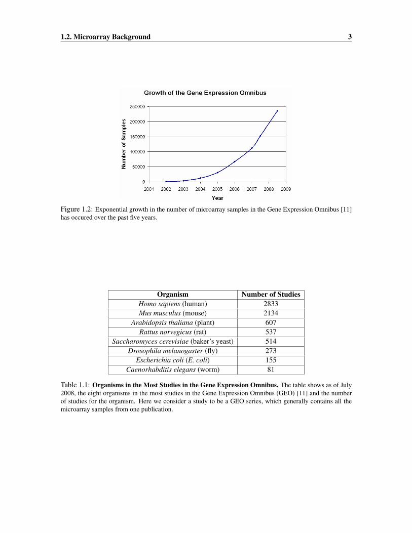
each gene in a sample to be quantified. As evidence of the growing importance microarray experi-
ments, the Gene Expression Omnibus (GEO) [11], one of the major public databases of microarray
experiments, has witnessed exponential growth in the number of microarray samples it contains
over the past five years. In Table 1.1 we also show for human and seven leading model organisms,
the total number of different studies containing microarray data for it in the GEO database [11].
1.2. Microarray Background 3
Figure 1.2: Exponential growth in the number of microarray samples in the Gene Expression Omnibus [11]has occured over the past five years.
Organism Number of StudiesHomo sapiens (human) 2833Mus musculus (mouse) 2134
Arabidopsis thaliana (plant) 607Rattus norvegicus (rat) 537
Saccharomyces cerevisiae (baker’s yeast) 514Drosophila melanogaster (fly) 273
Escherichia coli (E. coli) 155Caenorhabditis elegans (worm) 81
Table 1.1: Organisms in the Most Studies in the Gene Expression Omnibus. The table shows as of July2008, the eight organisms in the most studies in the Gene Expression Omnibus (GEO) [11] and the numberof studies for the organism. Here we consider a study to be a GEO series, which generally contains all themicroarray samples from one publication.
4 Chapter 1. Introduction
There exists two main types of microarrays, two channel cDNA (complementary DNA) ar-
rays and single channel oligonucleotide microarrays. In cDNA microarrays the probes contain
pre-synthesized sequences that are then placed on the array. These sequences can be hundreds of
base pairs long. Olignoucleotide microarrays contain sequences that are directly synthesized onto
the microarray. These sequences are shorter, for instance on the microarrays made by the com-
pany Affymetrix, olignucleotide sequences are only about 25 bases long [66]. Several different
oligonucelotide sequences are used to detect expression of each gene.
Figure 1.3 outlines the procedure for a two channel microarray experiment. RNA is first ex-
tracted from the two samples that will be directly compared on the microarray. The RNA is then
converted into cDNA by a process called reverse transcription. The cDNA from the different sam-
ples are then labeled with different colors, red and green. The microarray has thousands or tens
of thousands of spots with probes that will bind to specific cDNA sequences usually representing
genes. In a process called hybridization the cDNA is placed on the microarray and binds to specific
probes with complementary sequences. The hybridization process on the two channel arrays is a
competition between the two samples to determine which can bind a spot in greater quantity. The
microarray is then scanned and the color of the spots quantified. The color of a spot indicates for
which sample there is more corresponding cDNA present. For instance if more cDNA from the
sample labeled red binds the spot, then the spot will appear red when an image of the microar-
ray is scanned. We note two differences between experiments on single channel oliognucleotide
microarrays and the cDNA microarrays outlined in Figure 1.3, in a single channel oliognucleotide
microarray only one sample is hybridized to the microarray at a time and labeled cRNA is hybridized
to the microarray instead of cDNA.
1.3 Time Series Microarray Experiments
A key type of experimental data to understanding gene expression dynamics comes from time series
microarray experiments. Time series microarray experiments allow the measurement of the mRNA

1.3. Time Series Microarray Experiments 5
Figure 1.3: Outline of a cDNA Microarray experiment. The experiment begins with two different pop-ulations of cells (e.g. cells collected 1 hour before treatment and cells immediately before treatment). ThemRNA is isolated from both cells. The mRNA is then reverse transcribed into cDNA. The cDNA from onepopulation is labeled red, while for the other population it is labeled green. In a processed called hybridizationthe labeled cDNA is then placed on the microarray, and the cDNA bind to probes on the microarray with acomplementary sequence (A complements T and G complements C). The color of a spot indicates for whichof the two samples had greater quantity of the mRNA.
of every gene from a biological sample over multiple time points. These experiments are used
to study a range of dynamic biological processes such as the cell cycle [174], development [2],
environmental stress response [48], and immune response [58]. Based on our previous analysis of
the distribution of microarray experiment types in the Gene Expression Omnibus [11], we estimate
that approximately a third of all microarray studies involve time series experiments with three or
more time points [38]. An important property to note about time series microarray experiments
from our analysis is that most are short. We estimate that over 80% of time series experiments
contain no more than eight time points (Figure 1.4). An analysis of another database, the Stanford
Microarray Database [51] (SMD), found similar results (Figure 1.5) [40]. There are a number of
reasons why short time series datasets are so common. Time series experiments require multiple
arrays (and in some cases each point is repeated at least once) making them very expensive. While
microarray technology have greatly improved over the past decade, its cost is still high at around
$300-1000 per microarray sample, which is a limiting factor for many researchers. In some studies,
most notably clinical studies, the availability of biological material can limit the number of time

6 Chapter 1. Introduction
Figure 1.4: Distribution of microarray experiments by type. Summary of the 786 microarray datasets forhuman, mouse, rat, and yeast in the Gene Expression Omnibus in August 2005. As can be seen, 27.5% of thesets are time series experiments with 3-8 time points and roughly a third are time series data sets of 3 or moretime points. All of these sets were labeled as either time, development, or age in the database. An additional1% percent contains other types of sequential experiments including dose or temperature response, with 3-8different levels.
Figure 1.5: Distribution of lengths of times series in the Stanford Microarray Database in June 2004. Whiletime series are as long as 80 time points, the substantial majority have 8 or fewer time points.

1.4. Inferring the Location of Transcription Factor Binding 7
points collected. Thus, even if the price of microarray experiments were to go down short time
series expression experiments would remain prevalent.
1.4 Inferring the Location of Transcription Factor Binding
An important type of information towards understanding transcriptional regulation, is knowing
where in the genome a transcription factor binds. With knowledge of the location of transcrip-
tion factor binding one can then make inferences about the genes the transcription factor regulates,
as often the transcription factor will be regulating the nearby gene(s). In this section we first discuss
a computational approach to inferring the location of transcription factor binding, before moving on
to discuss some high-throughput experimental approaches.
1.4.1 Motif Scanning
position 1 2 3 4 5 6 7 8A 0 0 0 0 0 0 0 0C 0 0 0 4 2 10 0 9G 0 0 0 6 8 0 10 1T 10 10 10 0 0 0 0 0
Table 1.2: The Position Weight Matrix of the E2F transcription in the JASPAR database [183].
A computational approach to predicting where in a genome a transcription factor would bind is
based on motif-scanning. In this approach the sequence at each site is scored based on agreement
with the sequence binding preference of the transcription factor. A popular way to represent the
sequence binding preference is through a position weight matrix (PWM) (see Table 1.2) [50]. There
are about one thousand PWMs available between the JASPAR and TRANSFAC databases [109,
183]. The PWM matrix for a transcription factor is commonly formed by aligning the sequences
of a number of its confirmed binding sites, and then counting the frequency of each nucleotide
at each position. Additionally PWMs can be derived based on new high-throughput experimental
technology to determine the binding specificity of transcription factors [15, 121].

8 Chapter 1. Introduction
Under a PWM model, each position is considered independently, and the probability of seeing
a specific nucleotide at a specific position can be computed by taking the ratio of the count in the
matrix of that nucleotide at that position with the sum of the counts for all nucleotides at that posi-
tion. For instance the probability of observing a ‘C’ at position 4, based on the PWM in Table 1.2 is
0.4. To score a sequence, b1, ..., bW one takes the ratio of the probability of the sequence under the
PWM model, PWM, with the probability under a background model, BCKG. That is the score for
the sequence would be
∏Wi=1 p(bi|PWM, i)∏Wi=1 p(bi|BCKG)
(1.1)
If for instance the background model was a zero-order markov model where the probability of
an ‘A’ or a ‘T’ is 0.6 and the probability of a ‘C’ or a ‘G’ is 0.4 then the score given to the sequence
TTCGCGCC using the PWM in Table 1.2 would be
1.0 × 1.0 × 1.0 × 0.4 × 0.8 × 1.0 × 1.0 × 0.90.6 × 0.6 × 0.6 × 0.4 × 0.4 × 0.4 × 0.4 × 0.4
(1.2)
In practice a pseudo-count is also added to each entry in the matrix, which prevents a sequence
from having a score of 0 just because a specific nucleotide had not been observed previously at that
position. Usually when scanning a region of DNA, both strands are scanned, with the scanning of
the complementary strand done in the reverse direction.
Motif scanning is limited in that often there can be many sites which match well with the tran-
scription factor’s motif, but are not actually bound. One strategy to attempt to reduce the false
positives is by requiring the binding site be conserved [194] across multiple organisms, under the
assumption that a conserved site is more likely to have a function. In Chapter 5 we discuss a method
that integrates conservation along with several other evidence sources, to form a prior probability
that a location in the genome would represent a truly bound site.

1.4. Inferring the Location of Transcription Factor Binding 9
1.4.2 High-throughput Experimental Methods
Figure 1.6: Outline of the ChIP-chip, ChIP-Seq, and ChIP-PET methods for Locating TranscriptionFactor Binding. In the first step a chemical treatment is applied to crosslink the transcription factor to theDNA it is binding. Cells are then broken open and the DNA is sheared into smaller regions. An antibody forthe transcription factor of interest selects for only the DNA regions the transcription factor binds. The proteinand antibody are then removed from the DNA region. The three technologies then differ as to how theydetermine the location in the genome to which the DNA fragment corresponds. In the ChIP-chip method, theDNA fragments are hybridized to a microarray. In the ChIP-PET method, the ends of the DNA fragment aresequenced. In the ChIP-Seq method, lots of short reads from within the DNA sequence are obtained.
Figure 1.6 illustrates three experimental techniques, ChIP-chip, ChIP-Seq, and ChIP-PET, that
can be used on a genome-wide scale to determine the location of transcription factor binding (see
Figure 1.6). All three methods first rely on the technique of Chromatin Immunoprecipitation [144]
(ChIP), which isolates fragments of sequences in the genome that are bound by a transcription
factor. The methods differ in how they determine where in the genome the fragements of DNA
originated.
Chromating Immunoprecipitation works by chemically linking transcription factors to DNA,
such that fragments of DNA can be extracted from the cells with the transcription factors still linked
to the portions of DNA they were bound before extraction. An antibody specific to the transcription
factor of interest can then be used to isolate the specific DNA fragments that the transcription factor
bound. The antibody and transcription factor are then removed from the DNA.
The Chromatin Immunoprecipitation on chip (ChIP-chip) [144] method determines where in the

10 Chapter 1. Introduction
genome the DNA fragements originated by hybridizing the DNA sequences to a microarray. When
hybridized using a two-channel microarray the second channel contains DNA extracted from the
cell without using an antibody specific to the transcription factor. Only binding for sequences rep-
resented on the microarray can be detected. Some microarrays designed for ChIP-chip experiments
only provide coverage within promoters regions, that is regions of the genome near transcription
start sites of gene. Tiling microarrays are designed to cover an entire genome, though for larger
genomes such as Human, multiples microarray slides are needed to do so.
A more recent strategy that has been applied to determine where in the genome these DNA
fragements originated is to directly sequence them, and then map the sequence back to the genome.
In the Chromation Immunoprecipitation with paired-end ditag (PET) sequencing (ChIP-PET), 18
bases from each end of the DNA fragment are sequenced and then from this the location in the
genome that this fragment originated is determined [188]. An alternative sequencing method is the
ChIP-sequencing (ChIP-Seq) method [73, 146] where DNA fragments are sequenced using what are
referred to as next-generation sequencing platforms. These platforms provide lots of short sequence
reads (about 30 bases) on a DNA sample. To reduce false positives for both ChIP-PET and ChIP-
Seq, one requires the same region of the genome to be mapped multiple times before it is declared
a bound site.
There are several limitations to note about these technology. One limitation is the Chromation
Immunoprecipitation step can only be applied if there is antibody available that recognizes the tran-
scription factor. Another limitation in that since the binding of only one transcription factor can be
investigated at a time it is not realistic to determine the location of binding for a substantial number
of transcription factors across multiple conditions or multiple time points. Also these methods do
not determine the exact location of binding, but rather isolate binding to within a region from few
hundred bases up to around a thousand bases. A final limitation is that these methods have difficulty
detecting binding in repetitive regions of the genome where the sequences are non-unique.

1.5. Static Methods for Analysis of Gene Regulation 11
1.5 Static Methods for Analysis of Gene Regulation
While time series gene expression data provides dynamic information on the biological response,
most methods of analysis that are applied to the data, as we will discuss, ignore the dynamic nature
of the data. Due to the large number of genes that are profiled in an expression experiment, a
common method to analyze expression data is by using one of several clustering methods. Genes
which cluster together based on expression data are often co-regulated or involved in the same
biological process. Hierarchical clustering [37] along with other standard clustering methods such
as k-means [177] and self-organizing maps [176] are often used in practice. While these clustering
algorithms yielded many biological insights, they are not designed for time series data. Specifically,
all these methods assume that data at each time point is collected independently of each other,
ignoring the sequential nature of time series data.
In addition to clustering, there has been a lot of interest in using expression data to infer static
aspects of transcriptional gene regulation networks. One of the major early works in this area was
the application of learning Bayesian Networks from expression data to infer regulatory relationships
between genes [43]. Another notable work suggested using regression trees instead of Bayesian
networks [162]. The regression trees were used to map the expression of predicted regulators to
the expression levels of its regulated genes. Others have integrated gene expression data with motif
information [69, 135, 163] or ChIP-chip data [9]. These methods focused on finding gene modules,
that is sets of genes with similar expression that are regulated by the same set of transcription factors.
All of these methods, while applied to time series expression data, did not take advantage of the
sequential ordering of the time points and only provided a static view of gene regulation. Figure 1.7
illustrates two simplified versions of the types of views static methods give on gene regulation.
While such static views produced are useful, they provide limited insights into the dynamic nature
of transcriptional gene regulation. A major component of this thesis will be a method that does
provide a global dynamic view of transcriptional gene regulation (Chapter 3).

12 Chapter 1. Introduction
Figure 1.7: Two simplified example static views on gene regulation. (A) A directed graph between genes,where there is an edge if there exist a regulatory relationship. (B) A graph where there are two types ofnodes, regulators and sets of genes. An edge means the regulator regulates the sets of genes. This is a typeof view suggested in [9]. These two views do not give explicit indication of the dynamic nature of biologicalresponses.
1.6 Overview of Thesis
In Chapter 2 of this thesis we will discuss a clustering algorithm designed specifically for short time
series expression datasets. As will be discussed in that chapter a number of effective methods are
available for analyzing longer time series, but are less appropriate for the more common short time
series. A particular concern when analyzing short time series datasets with thousands (or tens of
thousands) of genes, is that many patterns can be expected to appear at random. Due to noise and
the small number of points for each gene, some of these patterns will be shared by many genes.
The clustering method that we will present is designed to distinguish between patterns that occur
because of random chance and clusters that represent a real response to the biological experiment.
We also describe in that chapter the software, the Short Time-series Expression Miner (STEM),
which implements this clustering method along with additional features.
In Chapter 3 we move from a method designed to identify significant temporal expression pat-
terns, to one that attempts to explain temporal expression patterns as the output of an underlying
dynamic regulatory network. Our method integrates time series expression data with static transcrip-

1.6. Overview of Thesis 13
tion factor-gene association data using an instance of Input-Output Hidden Markov Model [13] to
model these regulatory networks while taking into account their dynamic nature. Our method works
by identifying bifurcation points, places in the time series where the expression of a subset of genes
diverges from the rest of the genes. These points are annotated with the transcription factors regu-
lating these transitions resulting in a unified temporal map. The method has been implemented as
part of the software the Dynamic Regulatory Events Miner (DREM), and was then applied to study
several stress responses in yeast. Using DREM we were able to automatically infer many aspects of
the temporal responses, some of which were previously known while others were new predictions.
These new predictions range from low level predictions regarding the timing of specific interactions
to mechanistic predictions about the set of transcription factors controlling recovery from stress to
predictions related to phenotypic changes. The predictions having been experimentally validated
leading to new roles for transcription factors in controlling yeast response to stress.
For the results in yeast we relied on there being extensive ChIP-chip data available [60]. In
other important model organisms such as E. coli as well as in human such extensive experimental
coverage on the location of transcription factor binding is currently not available. We address this
problem for E. coli in Chapter 4 with a method that predicts genes regulated by a transcription
factor by using gene expression, sequence motif data, and curated experimentally validated targets.
The method takes a semi-supervsied learning approach by leveraging information about genes for
which it is not known whether or not the transcription factor regulates the gene. We then applied our
transcription factor-gene interaction predictions with DREM to a new time series gene expression
microarray data set for the aerobic-anaerobic shift in E. coli.
In Chapter 5 we address the issue of inferring computational predictions of transcription factor-
gene interactions in human. We only assume we have information about the sequence binding
preferences of a transcription factor, and do not assume we have known gene targets available for it.
Our method first learns a prior on transcription factor binding locations independent of any specific
motif information for a transcription factor. This prior maps a variety of features about a location
in a genome into a prior probability that a transcription factor will bind the location. We learn the

14 Chapter 1. Introduction
prior by using the locations of transcription factor binding for those transcription factors for which
full genome binding experimental have been conducted. We then show that by combining this prior
with motif information we can improve the prediction of transcription factor binding.
We conclude the thesis with conclusions on the work presented and possible future work. To
summarize the major contributions of this thesis, they are:
• A new clustering method specifically designed for the short time-series gene expression data
with a software implementation, STEM, that has been downloaded by more than 1000 re-
searchers (Chapter 2).
• A new method and software implementation, DREM, to model gene regulation dynamics
integrating time series gene expression data and transcription factor-gene association data.
Applications of DREM to study stress response in yeast leading to new experimentally con-
firmed predictions (Chapter 3).
• A new method to improve the prediction of transcription factor-gene associations in E. coli.
Also an application of these predictions with DREM to analyze a new time series expression
data set for the aerobic-anaerobic shift in E. coli (Chapter 4).
• An informative prior on transcription factor binding across the human genome learned by
integrating a variety of evidence sources, that when used in combination with binding mo-
tif information for a transcription factor improves improves predictions of bound promoter
regions (Chapter 5).

Chapter 2
Clustering Short Time Series GeneExpression Data∗
2.1 Introduction
As discussed in Chapter 1, time series microarray experiments are a popular method to study a
wide range of biological processes. A vast majority of these time series have the property of being
short (3-8 time points). Due to the large number of genes that are being profiled, most papers
presenting short time series data sets use one of several clustering methods to analyze their data.
Hierarchical clustering [37] along with other standard clustering methods (such as k-means [177]
and self-organizing maps [176]) are often used for this task. While these clustering algorithms
yielded many biological insights, they are not designed for time series data. Specifically, all these
methods assume that data at each time point is collected independently of each other, ignoring the
sequential nature of time series data. A number of clustering algorithms specifically designed for
time series expression data were later suggested. These algorithms include clustering based on the
dynamics of the expression patterns [141], clustering using the continuous representation of the
∗The content of this chapter is based on the papers [38, 40].
15

16 Chapter 2. Clustering Short Time Series Gene Expression Data
profile [8], and clustering using a Hidden Markov Model [159]. While these algorithms work well
for relatively long time series data sets (10 points or more) they are less appropriate for shorter
time series. As we discuss below (see also Results), these algorithms will overfit the data when
the number of time points is small. In addition, when analyzing short time series data sets with
thousands or more genes, many patterns can be expected to appear at random. Due to noise and the
small number of points for each gene, some of these patterns will be shared by many genes. Most
clustering algorithms cannot distinguish between patterns that occur because of random chance and
clusters that represent a real response to the biological experiment.
In this chapter we present an algorithm designed specifically for short time series data sets. Our
algorithm starts by selecting a set of potential expression profiles. These set of profiles cover the
entire space of possible expression profiles that can be generated by the genes in the experiment
and each represents a unique temporal expression pattern. Because we are dealing with a time
series experiment, and because it does not contain many points, a relatively small set of profiles
can be defined for such data. Next, each gene is assigned to its most closely matching profile. A
permutation test on the time points is then used to determine profiles with a significant number of
genes assigned. Significant profiles can either be analyzed independently or they can be grouped
into larger clusters (based on noise estimates from the data). The resulting profiles or clusters
of profiles are then analyzed using the Gene Ontology (GO) [3] annotations to determine their
biological function.
2.1.1 Related work
As mentioned above, there are many general clustering algorithms that have been applied to gene
expression data (see [139] for a review). However, these algorithms do not take into account the
sequential nature of time series expression data and thus are less appropriate for such data.
This observation has led a number of researchers to investigate methods of analysis specifically
designed for time series data. For instance Ramoni et al [141] suggests clustering genes based on
their dynamics. This method relies on regression and groups together genes whose dynamics can be

2.1. Introduction 17
expressed with roughly the same auto-regressive equation. While this method works well for long
time series, it is less appropriate for short ones. Even when using only two regression parameters
(the minimum required to distinguish between up and down trend) a five time points expression
experiment can only use the last three time points (the first two cannot be regressed). This may
lead to overfitting, and also results in poor cluster separation as we show in the Results section.
Bar-Joseph et al [8] presented a clustering algorithm that uses splines to cluster the continuous
representation of time series expression data. Again, this algorithm is less appropriate for short time
series. Even when only two spline segments are used, this algorithm assumes the estimation of five
parameters for each gene (and a few other class related parameters). This will clearly overfit if the
data set contain only a small number of points. Schliep et al [159] suggests clustering genes based
on a mixture of Hidden Markov Models (HMM). In an EM style algorithm genes are associated
with the HMM most likely to have generated their time courses, then the parameters of the HMMs
are estimated based on the genes associated with them. This algorithm assumes that the number of
time points are larger than the number of states (or nodes in each Markov chain). Thus, while this
algorithm works well for long time series data sets it is less appropriate for short ones.
Pre-defined profiles have been used in the past to fit expression profiles. For example, Zhao et
al [201] and Lu et al [99] have used sinusoids to identify cycling yeast genes. However, unlike our
method these profiles require the a-priori knowledge of the shape of the curve they wish to fit. In
most cases, such knowledge is not available. Moller-Levet et al [116] present a method in which a
comprehensive set of profiles is defined. Using these profiles genes are clustered by assigning them
to matching profiles. Unlike our method, their algorithm does not select a subset of the potential
profiles and so the number of profiles grows exponentially in the number of time points. Thus, their
algorithm is only appropriate for very short time series. In addition, their method cannot differentiate
between patterns arising from random noise and patterns representing biological response. Thus,
many of the resulting profiles do not represent true biological response. Peddada et al [131] suggests
a method to specify expression profiles based on inequality constraints. Genes are assigned to the
profile for which they best match as determined by a statistical procedure. Unlike our method, their

18 Chapter 2. Clustering Short Time Series Gene Expression Data
algorithm requires the user to specify the set of profiles in which she is interested. In addition, their
method requires several repeats. Such large number of repeats are usually not obtained in time series
experiments. Phang et al [134] also has a method that requires multiple full time series repeats to
assign genes to a set of pre-defined profiles. As with the method of Moller-Levet et al [116] the
number of profiles is exponential in the number of time points, and no method is suggested to select
a subset.
2.2 Identifying significant expression patterns
Our algorithm starts by selecting a set of potential profiles. Next, genes are assigned to the profile
that best represents them among the pre-selected profiles. We first discuss how to chose a represen-
tative set of profiles. Next, we discuss how we assign genes to profiles and how we determine the
significance of each of the profiles, and then finally how to group them.
2.2.1 Selecting model profiles
As discussed in the introduction we are interested in selecting a set of model expression profiles all
of which are distinct from one another, but representative of any expression profile we would likely
see. Here we assume that the raw expression values are converted into log ratios where the ratios are
with respect to the expression of the first time point. The first value of the series after transformation
will thus always be 0. To define a set of model profiles the user defines a parameter c that controls
the amount of change a gene can exhibit between successive time points. For example, if c = 2 then
between successive time points a gene can go up either one or two units, stay the same, or go down
one or two units. When using the correlation coefficient, as we do below, ‘one unit’ may be defined
differently for different genes. For n time points, this strategy results in (2c + 1)n−1 profiles. Note
that this method takes advantage of both the fact that we are dealing with a time series (resulting in
a limited set of values at the beginning compared to the end) and the fact that they are short (and so
n is small). For example, 5 time points and c = 1 would result in 34 = 81 model profiles. Since we

2.2. Identifying significant expression patterns 19
are dealing with thousands of genes, many genes will be assigned to each of the 81 profiles allowing
us to identify the significant profiles in this experiment.
While the above method generates a manageable number of profiles for short time series when
c = 1, the number of profiles grows as a high order polynomial in c. For example, for 6 time points
and c = 2 this method results in 55 = 3125 model profiles which are too much for any user to
view, and are also likely to be very sparsely populated. In such cases we are interested in selecting a
(manageable) subset of the profiles. Assume we are interested in m representative profiles. There are
a number of ways to select such a subset. Since the major purpose of the expression experiment is to
identify distinct patterns of gene expression (which are likely to correspond to different functional
categories), we would like to retain a distinct set of profiles. Computationally speaking, let P
represent the (2c + 1)n−1 set of possible profiles. We would like to select a set R ⊂ P with m profiles
(|R| = m) such that the minimum distance between any two profiles in R is maximized. Such a set
will guarantee that the profiles retained from P are as distinct as possible from each other. This
requirement can be formalized by selecting a subset R which maximizes the following function:
maxR⊂P,|R|=mminp1,p2∈Rd(p1, p2) (2.1)
where the distance, d, is a pseudometric. A pseudometric is a non-negative symmetric function
satisfying the triangle inequality (i.e. d(a, b) + d(b, c) ≥ d(a, c)). A pseudometric also satisfies the
property that d(x, x) = 0, but unlike for a metric it is not required that d(x, y) = 0 imply x = y.
For a set R we define
b(R) = minp1,p2∈Rd(p1, p2) (2.2)
That is, b(R) is the minimal distance between profiles in R, which is the quantity we wish to
maximize. Let R′ be the set of profiles that maximizes Equation 2.1. Thus, b(R′) is the optimal value
we can achieve. Unfortunately, as we prove below, finding such a set R′ that maximizes this function
is NP-Hard. Moreover, an approximation that guarantees a solution that is better than b(R′)/2 is

20 Chapter 2. Clustering Short Time Series Gene Expression Data
also NP-Hard. The proof of both claims rely on a reduction from the maximal independence set
problem. We note that we are proving the result for the general setting of a pseudometric on a set
of elements, depending on the additional assumptions about the relationship between elements and
the pseudometric in some cases the problem may not be NP-Hard.
Lemma 2.2.1. For a set of elements V, a set R ⊂ V, and a pseudometric d, let b(R) = minv1,v2∈Rd(v1, v2).
Set b′ = maxR⊂V,|R|=mb(R). Then finding a set R such that |R| = m and b(R) = b′ is NP-Hard. Fur-
thermore finding a set R such that |R| = m and b(R) > b′2 is also NP-Hard.
Proof. We first note that given an undirected graph (V, E) the problem of finding an independent set
of size m, that is a subset of m vertices such that there is no edge between any two vertices in the
subset, is NP-Hard [63]. We will define the pseudometric d′ in R to be:
d′(u, v) =
0 if(u = v)
1 if(u , v) ∧ ((u, v) ∈ E)
2 if(u , v) ∧ ((u, v) < E)
Note that all requirements of a pseudometric are trivially satisfied except the triangle inequality,
d(x, z) ≤ d(x, y)+d(y, z). To verify the triangle inequality also holds, note that for any two elements,
x and z, the possible values of d′(x, z) are 0, 1, and 2. If d′(x, z) = 0 then the triangle inequality
is trivially satisfied since d′ is non-negative. If d′(x, z) = 1 and the triange inequality was not
satisfied, we would have d′(x, y) = 0 and d′(y, z) = 0, which would imply x = z and d′(x, z) = 0
contradicting d′(x, z) = 1. If d′(x, z) = 2 and the triangle inequality was not satisfied, then we have
d′(x, y) + d′(y, z) ≤ 1, which means either d′(x, y) = 0 or d′(y, z) = 0. Without loss of generality
assume d′(x, y) = 0, then we have x = y and d′(y, z) = d′(x, z) = 2, which gives a contradiction.
Thus the triangle inequality is satisfied in all cases.
We observe that if R is a subset of V of size m such that b(R) = b′ and b(R) > 1, then the
subset of vertices of V which are also elements of R must form an independent set of size m.
Furthermore we observe that if b(R) ≤ 1, then there is no independent set in V of size m. We

2.2. Identifying significant expression patterns 21
have thus reduced independent set to being an instance of our problem hence finding an optimal
solution to our problem is NP-Hard. Furthermore if we could find a subset R of V of size m for
which it is guaranteed that b(R) > b′2 in polynomial time, then by the same reduction we could
solve independent set in polynomial time, and thus the problem of finding an approximation which
guarantees b(R) > b′2 in polynomial time is NP-Hard. �
Thus, unless P = NP, the best polynomial algorithm for this problem can only guarantee a set
R which achieves a value of b(R′)/2. We now present a greedy algorithm that is guaranteed to find
such a set. That is, our algorithm finds a set of profiles R, with b(R) ≥ b(R′)/2. Our algorithm
(presented in Figure 2.1) starts with one of the two types of extreme profiles (going down at each
time point). Let R be the set of profiles selected so far. The next profile added to R is the profile p
that maximizes the following equation:
maxp∈(P\R)minp1∈Rd(p, p1) (2.3)
that is, in each iteration we selects a profile that is the furthest from all profiles selected so far (R).
This selection is repeated until m profiles have been selected and the resulting set is returned. The
left image of Figure 2.4 illustrates the profiles selected when m = 50 and c = 2.
procedure SelectElementsMaxMinDist(d,P,m)let p1 be the profile that always goes down one unit between time pointsR = {p1}; (? The set of selected elements ?)L = P \ {p1};for i = 2 to m do
let p ∈ L be a profile that maximizes:minp1∈Rd(p, p1);
R = R ∪ {p}; L = L \ {p};end for;return R;
Figure 2.1: Greedy approximation algorithm to choose a set of m distinct profiles
The following theorem proves our claim about the lower bound on b(R) for this algorithm:

22 Chapter 2. Clustering Short Time Series Gene Expression Data
Theorem 2.2.1. Let d be a pseudometric. Let R′ ⊂ P be the set of profiles that maximizes Equa-
tion (2.1). Let R ⊂ P be the set of profiles returned by our algorithm, then b(R) ≥ b(R′)2 .
This theorem is proved by considering two cases regarding the relationship between the set of
profiles identified by the our algorithm (R) and the optimal set (R′). For both cases we show below
that there exists a profile p ∈ R that is at a distance at most b(R) from two different profiles from R′.
Thus, we can use the triangle inequality to show that b(R′) is at most twice b(R).
Proof. Set b′ = b(R′) (b′ is the optimal distance) and b = b(R) (b is the distance returned by our
algorithm). Let {r′1, r′2, ..., r
′m−1, r
′m} be the profiles in R′ and {r1, r2, ..., rm−1, rm} be the profiles in R.
Note that for any profile p ∈ P there exists a profile r j ∈ R such that d(p, r j) ≤ b. If p is one of the
profiles in R then let r j = p, which gives d(p, r j) = d(r j, r j) = 0 ≤ b. If p < R then there must be
a profile in R with a distance at most b from p otherwise the greedy algorithm would have selected
p from R instead of rm (we know that the minimum distance b was achieved by the last profile rm).
For each profile in R′ we can find its closest profile in R. Next, we consider two possible cases,
which are also the only possible cases:
Case 1 - Two different profiles, r′i , r′j ∈ R′, are closest to the same profile rh ∈ R:
We note that d(r′i , rh) ≤ b and d(r′j, rh) ≤ b as mentioned above. Using the triangle inequality we get
2b ≥ d(r′i , rh) + d(r′j, rh) ≥ d(r′i , r′j) ≥ b′ and thus our solution is at least half of an optimal solution.
Case 2 - No two profiles in R′ are closest to the same profile in R:
WLOG let r′m be the profile which is closest to rm (the last profile added by our algorithm). We next
observe that there must exists i , m such that d(r′m, ri) ≤ b. This is so because if such a profile ri
did not exist then the greedy algorithm would have selected r′m instead of rm. Let r′i be the profile
from R′ closest to ri, then d(r′i , ri) ≤ b since all profiles are within b of a profile selected by the
greedy algorithm. We thus have 2b ≥ d(r′m, ri) + d(r′i , ri) ≥ d(r′i , r′m) ≥ b′ which again shows that
our solution is at least half of an optimal solution. �
The above algorithm performs m iterations and each of these takes at most m(2c + 1)n−1 time for
a total running time of O(m2(2c + 1)n−1). Since m is small (m should be at most 100 in order to be

2.2. Identifying significant expression patterns 23
manageable), the total running time of this algorithm is small for short time series data sets (small
n).
It is interesting to briefly discuss a related problem known as the k-centers problem [63]. In our
notations, the k-centers problem tries to find a group R that minimizes the following equation:
minR⊂P,|R|=kmaxp1∈P\R,p2∈Rd(p1, p2) (2.4)
In other words, we are looking for a subset R of size k such that the maximum distance from points
not in R to points in R is minimized. The k-centers problem tries to select centers that are the best
representatives for the group while our goal is to find the most distinct profiles. While in general
an optimal solution to one of these problems is not necessarily an optimal solution to the other, the
algorithm we presented above is also known to be the best possible approximation algorithm for
k-centers (the proof is obviously different). Thus, this algorithm provides the best of both worlds: a
distinct subset that is also a good representation of the initial set of profiles P.
2.2.2 Identifying significant model profiles
Given a set M of model profiles, and a set of genes G, each gene g ∈ G is assigned to a model
expression profile mi ∈ M such that d(eg,mi) is the minimum over all m ∈ M. Here eg is the
temporal expression profile for gene g. If the above distance is minimized by h > 1 model profiles
(i.e. we have ties) then we assign g to all of these profiles, but weight the assignment in the counts
as 1/h. We count the number of genes assigned to each model profile and denote this number for
profile mi by t(mi).
Next, we would like to identify model profiles that are significantly enriched for genes in our
experiment. Our null hypothesis is that the data is memoryless. That is, the probability of observing
a value at any time point is independent of past and future values. Thus, according to the null
hypothesis, any profile we observe is a result of random fluctuation in the measured values for genes
assigned to that profile. Model profiles that represent true biological function deviate significantly

24 Chapter 2. Clustering Short Time Series Gene Expression Data
from the null hypothesis since many more genes than expected by random chance are assigned to
them.
Determining a parametric model for our null hypothesis is complicated by the many noise fac-
tors that affect gene expression measurements. Instead, we follow many previous methods for static
gene expression analysis [35, 180] and use a permutation based test. In our case, permutation is used
to quantify the expected number of genes that would have been assigned to each model profile if the
data was generated at random. Note that under the null hypothesis, the order of the observed values
is random (as each point is independent of any other point) and thus permutations are expected to
result in profiles that are similar to the null distribution.
Since there are n time points, each gene has n! possible permutations, and all of these can be
computed for small values of n. For each possible permutation we assign genes to their closest
model profile. Let s ji be the number of genes assigned to model profile i in permutation j ( j is one
of the n! possible permutations). We set S i =∑
j s ji . Then, Ei = S i/(n!) is the expected number
of genes for each profile model if the data was indeed generated according to the null hypothesis.
Note that different model profiles may have different number of expected genes and so in general
Ei , |G|/m (see Results).
Since each gene is assigned to one of the profiles, we can assume that the number of genes
in each profile is distributed as a binomial random variable with parameters |G| and Ei/|G|. Thus
the (uncorrected) p-value of seeing t(mi) genes assigned to profile pi is P(X ≥ t(mi)) where X ∼
Bin(|G|, Ei/|G|). If we were testing just one model expression profile for significance then we could
consider the number of genes assigned to pi to be statistically significant at the α significance level
if P(X ≥ t(mi)) < α. However since we are testing m model profiles for significance, we need
to correct for the multiple comparisons. We thus apply a Bonferroni correction and consider the
number of genes assigned to pi to be statistically significant if P(X ≥ t(mi)) < α/m. The running
time of the permutation test method is |G|n!m which for small m and n is at most quadratic in the
number of genes.

2.2. Identifying significant expression patterns 25
2.2.3 Correlation Coefficient
While the profile selection algorithm and approximation guarantee of Section 2.2.1 works with any
pseudometric, in this thesis we suggest the use of a pseudometric based on the correlation coefficient
ρ(x, y). The correlation coefficient has enjoyed great success in computational biology, especially
when used in a clustering algorithm [37]. An advantage of the correlation coefficient for our method
is that it can group together genes with similar expression profiles even if their units of change are
different. However the correlation coefficient takes negative values and thus is not a pseudometric.
Fortunately the following simple transformation of the correlation coefficient:
d(x, y) =√
1 − ρ(x, y) (2.5)
does satisfy the requirements of a pseudometric, as we will show.
As the largest value the correlation coefficient takes is 1, d will always take on non-negative real
values. The symmetry of d follows directly from the symmetry of the correlation coefficient. Since
ρ(x, x) = 1, we have d(x, x) = 0. We will now prove a lemma to establish that d satisfies the triangle
inequality requirement of a pseudometric.
Lemma 2.2.2. Let d(x, y) =√
1 − ρ(x, y) where ρ(x, y) is the correlation coefficient, then d satisfies
the triangle inequality.
Proof. By definition the correlation coefficient can be written as
ρ(x, y) =< ψ(x), ψ(y) > (2.6)
where < ·, · > is a dot product, and
ψ(z) =
(z1 − z√
n × σz, ...,
zn − z√
n × σz
)(2.7)
In the above expression z = (z1, ..., zn) and z and σz are the mean and standard deviation respectively

26 Chapter 2. Clustering Short Time Series Gene Expression Data
of {z1, ..., zn}. As ρ is a dot product it is also an inner product. In general for an inner product we
have a norm defined as
||a|| =√< a, a > (2.8)
Also, in general if there is a norm then there is a distance metric induced as ([106]):
d(a, b) = ||a − b|| (2.9)
By letting a = ψ(x) and b = ψ(y) in Equation 2.9 and then applying Equation 2.8 it thus follow that
√< ψ(x) − ψ(y), ψ(x) − ψ(y) > (2.10)
is a distance metric and hence satisfies the triangle inequality. The above expression can also be
written as
√< ψ(x), ψ(x) > −2 < ψ(x), ψ(y) > + < ψ(y), ψ(y) > (2.11)
As the correlation of a vector with itself is 1, the above expression reduces to
√2 − 2 < ψ(x), ψ(y) > (2.12)
=√
2√
1− < ψ(x), ψ(y) > (2.13)
As d(x, y) =√
1 − ρ(x, y) =√
1− < ψ(x), ψ(y) > is within a scalar multiple of the above expression,
which satisfies the triangle inequality, it follows that d must as well. �
We note that when using the correlation coefficient, the constant 0 profile is excluded from
the set of model profiles, since the correlation coefficient is undefined when the standard deviation
is 0. Often non-differentially expressed genes are filtered prior to clustering anyway. Also for

2.2. Identifying significant expression patterns 27
some model profiles, x and y, where x , y we have d(x, y) = 0 (e.g. x = (0, 1, 2, 3, 4) and y =
(0, 2, 4, 6, 8)). We thus require the number of profiles m to be small enough such than m profiles can
be selected such that minimum distance between any two selected profiles, b(R) (see Equation 2.2),
is strictly greater than 0.
2.2.4 Grouping Significant Profiles
The assignment of genes to model profiles is deterministic. However, due to noise, it is impossible
to rule out close profiles (even if not the closest) as being the true profile for individual genes. If we
have a measurement of the noise (for example from repeat experiments) it is possible to determine a
distance threshold δ below which two model profiles are considered similar (the difference between
genes assigned to these two may be attributed to noise). Such model profiles represent similar
enough expression patterns and thus should be grouped together.
In order to determine which model profiles should be grouped together we transform this prob-
lem into a graph theoretic problem. We define the graph (V, E) where V is the set of significant
model profiles, and E is the set of edges. Two profiles v1, v2 ∈ V are connected with an edge if
and only if d(v1, v2) ≤ δ. Cliques in this graph correspond to sets of significant profiles which are
all similar to one another. There are many ways to partition a graph into a set of cliques. Here we
are interested in identifying large cliques of profiles which are all very similar to each other. This
leads naturally to a greedy algorithm to partition the graph into cliques and thus to group significant
profiles.
The greedy algorithm we use to group profiles grows a cluster Ci around each profile pi in V .
Initially, Ci = {pi}. Next, we look for a profile p j such that p j is the closest profile to pi that is not
already included in Ci. If d(p j, pk) ≤ δ for all profiles pk ∈ Ci we add p j to Ci. We continue to
consider p j in order of increasing distance to pi, until no p j satisfying the criteria can be added, and
then we stop and declare Ci as the cluster for pi. After growing a cluster around each profile in V ,
we select the cluster with the largest number of genes (by counting the number of genes in each of
the profiles that are included in this cluster), remove all profiles in that cluster from V and repeat

28 Chapter 2. Clustering Short Time Series Gene Expression Data
Figure 2.2: Simulated data example. (Top Left) Expected vs. assigned number of genes for our first exper-iment. Points above the diagonal line correspond to profiles determined by our algorithm to be significantlyenriched. The horizontal line corresponds to the same significance level if we assume that the number of ex-pected genes for all profiles is the same. As can be seen our algorithm correctly determined that no profile issignificantly enriched for genes, even though a number of profiles are above the horizontal line. (Top Right)Similar plot for our second experiment. Our algorithm correctly identified all three planted profiles, eventhough each was planted with only 1% of the genes. (Bottom) The three significant profiles found out of theset of fifty considered. The fifty profiles considered are the same as appear in Figure 2.4.
the above process. The algorithm terminates when all profiles in V have been assigned to clusters.
The running time of this algorithm is O(|V |4), where |V | is the number of significant profiles, which
is generally small.
2.3 Results
We present results for both simulated and biological data. We first present results on two simulated
data sets illustrating empirically that our method performs consistently with theoretical expectations.
We then on a batch set of simulated data, illustrate differences between our method and the k-
means clustering algorithm. Finally, we present results for using our algorithm to study the immune
response system in humans. For this data we have also compared our results with the k-means
clustering algorithm and the CAGED clustering method [141], which is designed for clustering
time series expression data.
Simulated Data Set Example

2.3. Results 29
We generated a data set simulating 5,000 genes with five time points. The raw expression value
at each time point for a gene was randomly drawn from a Uniform[10,100] distribution (other dis-
tributions yielded similar results). Each value was drawn independently of all other values, and the
distribution was identical for all time points. Next we transformed this data to a log ratio represen-
tation. We applied our algorithm using 50 model profiles with a maximum unit change between
time points of two. As expected, our algorithm determined that none of the profiles had a significant
number of genes. Figure 2.2 (top left) plots the number of genes assigned to each profile against
the number of genes expected. The region above the diagonal line corresponds to gene assignments
levels that would be statistically significant at an α = 0.05 Bonferroni corrected level or equivalently
at an α = 0.001 uncorrected level. Note that if we assume that the number of expected genes for
each profile is the same (5000/50 = 100 in our case), then anything above the horizontal line would
be considered statistically significant. The distribution of profiles on the graph illustrates that differ-
ent temporal expression profiles are more likely than others to occur by random chance, something
which standard clustering algorithms do not take into account.
In our second experiment we selected three profiles, as appear in Figure 2.2 (bottom), and as-
signed 50 genes (1%) to each of these profiles with some noise (the other 4850 genes were generated
as described above). For genes planted to a profile, (p0, p1, p2, p3, p4), their raw expression values
were generated by generating (v0, v1, v2, v3, v4) where
vt =
U0 if(t = 0)
vt−1 × (2pt−pt−1) + Yt if(t > 0)
U0 is a random variable for a Uni f orm[10, 100] distribution and Yt is a random variable for a
Uni f orm[−0.05×2pt−pt−1 , 0.05×2pt−pt−1] distribution. The log ratio with v0 was then taken for each
value. Figure 2.2 (top right) shows the results obtained for this data. The only three profiles which lie
above the diagonal line are those for which the genes were planted. Thus, all three selected profiles
were correctly recovered by our algorithm, and no other profile was determined to be significant.
Note that the significant profiles had roughly half the number of genes assigned than a number of

30 Chapter 2. Clustering Short Time Series Gene Expression Data
Figure 2.3: Batch simulated data results. (Left) The black line in the graph shows for each number ofmodel profiles from 2-100 the average number of declared significant profiles across the 100 simulated datasets. The red lines represents points either two standard deviations above or below the average. The numberof simulated real clusters was 5. (Right) In this figure we compare three methods for forming clusters ofgenes: genes assigned to the same significant profiles, genes assigned to the same profile (significant ornot), and genes belonging to the same k-means cluster. For each method we are comparing the total numberof clusters the method produces against the average best agreement of each real simulated cluster with acluster produced by the method (formally the hS (R) value defined in the text). The image shows that whenthe number of clusters from a method is in the range of the actual number of true clusters (5), the clustersformed based on the significant profiles have the best agreement with the real simulated clusters. When k isgreater than about 25, the k-means clustering method can form some clusters with better overlap with the realsimulated cluster than the significant profiles method can for any number of significant profiles. However insuch cases the k-means clustering method is also forming many additional clusters of genes which representnoise.
non-significant profiles. Such smaller, but more statistically significant cluster of genes could be
overlooked by a traditional clustering algorithm.
Results on a Batch Set of Simulated Data
Our next set of experiments were conducted on a batch set of 100 simulated data sets. In these
experiments we also compare with the k-means clustering algorithm. In each of the simulated data
sets there were 5000 genes measured at 5 time points. Each simulated data set had 4500 noise
genes. To generate the simulated log-ratio expression value of these noise genes in log-space we
first generated for t = 0, 1, 2, 3, 4:
vt = 2 × Yt (2.14)
where the Yt are random variables sampled from a standard normal distribution. We then used the

2.3. Results 31
following as the simulated log-ratio values:
(0, v1 − v0, v2 − v0, v3 − v0, v4 − v0) (2.15)
The remaining 500 genes were planted with noise into one of five simulated real clusters with
100 genes planted into each. To generate the log-ratio expression values of a set of 100 genes
belonging to one of these simulated real cluster we first generated a vector (p0, p1, p2, p3, p4) based
on the following equation:
pt =
Zt if(t = 0)
pt−1 + Zt if(t > 0)(2.16)
where the Zt are random variables drawn from a standard normal distribution. For each of the 100
genes belonging to this cluster we generated for t = 0, 1, 2, 3, 4:
vt = pt + 0.25 × Yt (2.17)
where the Yt are random variables sampled from a standard normal distribution. Finally we applied
the same transformation as in Equation 2.15 for each gene.
After generating these 100 data sets, we ran both our clustering method and the k-means clus-
tering algorithm on these data sets. We ran our clustering method for every value of the number of
model profiles between 2 and 100. We set the parameter for the maximum unit change between time
points (c) to 2. We set the significance level to a Bonferonni corrected significance level of 0.05.
For the k-means algorithm we used the Matlab 7.5 implementation using the ‘correlation’ distance
function. We ran k-means for every value of k from 2 to 100.
Figure 2.3 (left) shows for each number of model profiles using our method, the average number
of these profiles identified as significant across the 100 simulated data sets, along with a 2-standard
deviation interval around this. We observe for about 50 or more initial model profiles the number of
significant model profiles identified falls tightly in the 4-5 range. This is reasonably consistent with

32 Chapter 2. Clustering Short Time Series Gene Expression Data
there being five simulated real clusters in the data.
We next evaluated how well the genes planted into the simulated real clusters overlapped with
the set of genes assigned to the significant model profiles. Let S denote the set of sets of genes
assigned to the same significant profile. Let R denote the set of sets of genes planted into the same
cluster. For each set r ∈ R we computed its best Jaccard index with any set s ∈ S . The Jaccard
index which measures overlap between two sets is the ratio of the size of the intersection between
two sets divided by its union. Formally we define
jS (r) = maxs∈S|r ∩ s||r ∪ s|
(2.18)
We then computed the median value of jS (r) across the five simulated real clusters, that is we define
hS (R) to be
hS (R) = median{ jS (r)|r ∈ R} (2.19)
We repeated the same procedure where instead of using for S the set of sets of genes assigned
to the same significant model profile, we used the set of sets of genes assigned to the same model
profile (significant or not). We also repeated the procedure where S was the set of set of genes
assigned to the same k-means cluster. In Figure 2.3 (right) we compare the average value of hS (R)
against the size of S , for the three different ways we defined S . In this figure we observe that for
values of |S | in the range 2-8, defining S based on the set of significant profiles leads to the highest
average hS (R). There was no case in which more than 8 profiles were considered significant. As
the k-means clustering algorithm forms clusters in a data dependent manner when k is sufficiently
large, it is able to achieve higher hS (R) values. However in such cases the k-means algorithm is also
forming many clusters that just represent random noise.
Biological Results
We tested our algorithm on immune response data from Guillemin et al [58]. In the paper the
authors used human cDNA microarrays to study the gene expression program of gastric AGS cells

2.3. Results 33
Figure 2.4: Biological data results. (Top) The main overview of the results as displayed in the Short Time-series Expression Miner (STEM) software (Section 2.4). The image shows 50 distinct temporal model profileswith a maximum unit change of two between time points is shown. The shaded profiles are statisticallysignificant. Profiles of the same shade are grouped together. The algorithm was able to narrow the 50 initialprofiles, to only 10 which were statistically significant. (Bottom) A plot of the number of genes assigned toeach profiles versus the expected number of genes. The ten points above the diagonal line are those which areconsidered statistically significant. One of these profiles, profile 14, lies well below the horizontal line andwould not be considered statistically significant if the number of genes assigned to each profile was assumedto be the same.
infected with various strains of Helicobacter pylori. Helicobacter pylori is one of the most abundant
human pathogenic bacteria. In this chapter we will analyze data from the response of the wildtype
G27 strain. We use data obtained from two replicates on the same biological sample in which time
series data was collected at five time points, 0 hours, 0.5h, 3h, 6h, and 12h.
We first selected 2243 genes for further analysis from the 24,192 array probes. Genes were
selected based on the agreement between the two repeats and their change at any of the experiment
time points (see supporting website of [40] for details). We used a set of 50 model profiles (using
more profiles yielded similar results, however, we believe that 50 is a manageable number and so
we focus on this set here). For the results discussed below we generated the model profiles using
a value of 2 for the maximum unit change parameter (c). Additional experiments with c = 1 and
c = 3 returned very similar results (see supporting website of [40] for details). Of the 50 model
profiles, 10 profiles in seven clusters were identified as significant. Figure 2.4 presents an image
and plot of the clusters and profiles. Shaded profiles are significant and profiles with the same
color belong to the same cluster. We used a correlation of 0.7 (δ = 0.3) in our grouping method.
Of the seven cluster of profiles one contained three profiles, one contained two profiles, and five

34 Chapter 2. Clustering Short Time Series Gene Expression Data
were single profiles. Four of the 10 significant model profiles were significantly enriched for Gene
Ontology (GO) categories (as determined by the hypergeometric distribution), two of these profiles
were assigned to the cluster containing three profiles while the other two remained separate. We
note that the array contained many un-annotated genes, which could explain why not all profiles
were significantly enriched for GO categories. Below we describe some of the significant profiles,
and discuss their relevance to GO categories for which the profiles were enriched.
Profile 9 (0,−1,−2,−3,−4) (see Figure 2.5) contained 131 genes that were down regulated
during the entire experiment duration. This profile was significantly enriched for cell cycle genes
(p-value < 10−10). Many of the cycling genes in this profile are known transcription factors, which
could contribute to repression of cell cycle genes, and, ultimately, the cell cycle [58, 110, 169].
Profile 14 (0,−1, 0, 2, 2), contained 49 genes. This profile is interesting since the raw number of
genes assigned to the profile is not large and thus it could be missed by a clustering algorithm which
ignores the sequential nature of the time series data. Genes assigned to this profile went slightly
down at the beginning but later were expressed at high levels. GO analysis indicates that many of
these genes were relevant to cell structure and annotated as belonging to the categories cytoskeleton
(p-value < 10−4), extracellular matrix (10−3), and membrane (10−5). Structural elongation of cells is
a known phenotypical response to pathogens, and thus the enrichment of such genes in up-regulated
expression profile is consistent with this biological response [58, 68]. Profile 41 contained 86 genes
that were going up during the entire experiment (0, 1, 2, 3, 4). The most enriched GO category for
this profile was response to stimulus (p-value < 10−4) which contains defense and immune response
genes. Since the experiment involved pathogen infection, such a reaction from immune response
genes is to be expected, and many of the un-annotated genes in this profile might be also related to
immune response.
We note that while the biological analysis in [58] was largely anecdotal (focusing on a few key
genes) many of these genes correspond to the above GO categories or to GO categories associated
with the other significant profiles. Thus our work contributes a rigorous statistical justification for
many of the observations made in that paper.

2.3. Results 35
Figure 2.5: CAGED and profile based clusters A cluster from CAGED (top left) containing all Profile14 (top right) genes and a substantial majority of Profile 41 (bottom left) genes, among many other genes.As can be seen, the fact that so many genes are grouped together masks the presence of significant profilesidentified by our algorithm resulting in low correlation with the relevant GO categories. Profile 9 is on thebottom right.
We compared our method with both, a general clustering algorithm (k-means) and an algo-
rithm, designed specifically for time series data (CAGED) [141]. We did not compare directly with
hierarchical clustering since hierarchical clustering does not give a fixed number of clusters (cut-
ting hierarchical clustering at a particular level in the tree resulted in few large clusters and many
singletons). For k-means we used the Matlab 6.5 implementation of k-means with the correlation
coefficient as the distance function (similar results were obtained when using Euclidean distance).
Since k-means does not assign significance to the clusters it detects we used two version of k-means
for this comparison. In the first version we clustered the entire set of 2,243 genes with 10 clusters.
In the second method we generated 50 clusters and selected the 10 clusters with the most genes for
further analysis. We used the third level of the GO hierarchy to compare our results with k-means.
For each clustering result we computed the GO enrichment for the selected clusters, and compared
them to the enrichment detected using our profiles algorithm. Sixteen third level GO categories had
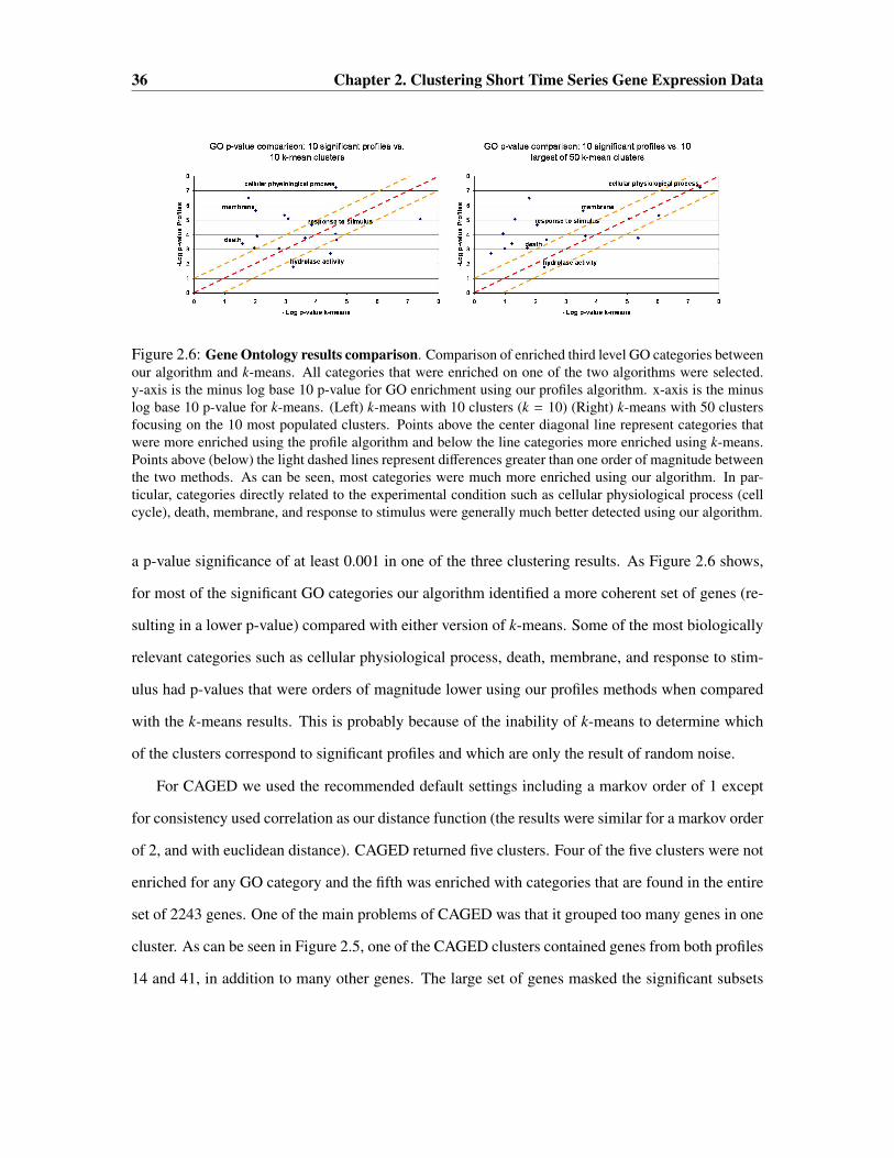
36 Chapter 2. Clustering Short Time Series Gene Expression Data
Figure 2.6: Gene Ontology results comparison. Comparison of enriched third level GO categories betweenour algorithm and k-means. All categories that were enriched on one of the two algorithms were selected.y-axis is the minus log base 10 p-value for GO enrichment using our profiles algorithm. x-axis is the minuslog base 10 p-value for k-means. (Left) k-means with 10 clusters (k = 10) (Right) k-means with 50 clustersfocusing on the 10 most populated clusters. Points above the center diagonal line represent categories thatwere more enriched using the profile algorithm and below the line categories more enriched using k-means.Points above (below) the light dashed lines represent differences greater than one order of magnitude betweenthe two methods. As can be seen, most categories were much more enriched using our algorithm. In par-ticular, categories directly related to the experimental condition such as cellular physiological process (cellcycle), death, membrane, and response to stimulus were generally much better detected using our algorithm.
a p-value significance of at least 0.001 in one of the three clustering results. As Figure 2.6 shows,
for most of the significant GO categories our algorithm identified a more coherent set of genes (re-
sulting in a lower p-value) compared with either version of k-means. Some of the most biologically
relevant categories such as cellular physiological process, death, membrane, and response to stim-
ulus had p-values that were orders of magnitude lower using our profiles methods when compared
with the k-means results. This is probably because of the inability of k-means to determine which
of the clusters correspond to significant profiles and which are only the result of random noise.
For CAGED we used the recommended default settings including a markov order of 1 except
for consistency used correlation as our distance function (the results were similar for a markov order
of 2, and with euclidean distance). CAGED returned five clusters. Four of the five clusters were not
enriched for any GO category and the fifth was enriched with categories that are found in the entire
set of 2243 genes. One of the main problems of CAGED was that it grouped too many genes in one
cluster. As can be seen in Figure 2.5, one of the CAGED clusters contained genes from both profiles
14 and 41, in addition to many other genes. The large set of genes masked the significant subsets

2.4. Software Implementation - Short Time Series Expression Miner 37
that were contained in this profile, resulting in no significant GO category for this cluster. While
CAGED is a very useful algorithm for long time series data sets, for short ones it seems like it does
not have enough data to further separate the clusters. In contrast, our algorithm looks at all possible
profiles (or a representative subset of them) allowing it to detect significant expression profiles even
if only a small number of genes are associated with them.
2.4 Software Implementation - Short Time Series Expression Miner
The algorithm in the previous section has been implemented as part of the Short Time-series Ex-
pression Miner (STEM), the first software application designed specifically for the analysis of
short time series gene expression data sets. The STEM software has additional features that we
will briefly discuss, for more details consult [38] and the manual on the STEM website (http:
//www.sb.cs.cmu.edu/stem). STEM is integrated with the Gene Ontology (GO) [3] which al-
lows for enrichment analyses for sets of genes having the same temporal expression pattern (Fig-
ure 2.7). Integrating in GO enrichment analysis into the software allows for an efficient and statisti-
cally rigorous biological interpretation of significant temporal expression patterns.
The integration of STEM with GO is bidirectional. STEM can easily determine and visualize
the behavior of genes belonging to a given GO category, identifying which temporal expression
profiles were enriched for genes in that category (Figure 2.8). In addition while the GO annotations
are provided directly to the user, a user can also supply their own gene sets to STEM and use them
as well.
Another feature of STEM is that it supports the ability to compare temporal responses of genes
across experimental conditions. In particular STEM can automatically identify pairs of profiles with
a significant overlap of the genes assigned to each profile (Figure 2.9).
Since its June 2005 release, STEM has been downloaded by more than 1000 researchers. Results
obtained by others analyzing new time-series microarray data sets using STEM have appeared in a
variety of biological journals [71, 96, 100, 107, 145, 160, 198].

38 Chapter 2. Clustering Short Time Series Gene Expression Data
Figure 2.7: Gene Ontology enrichment analysis table. The image shows an example of a GO enrichmentanalysis table. The first two columns of the table are the GO category ID and name. The third columncontains the total number of genes of each GO category on the microarray. The fourth column contains foreach GO category, the total number of genes on the microarray that were also assigned to the profile. The fifthcolumn contains the number of genes of that GO category that were expected to be assigned to the profile,in this case computed based on the profiles actual size. The sixth column contains how many more geneswere assigned than expected. The seventh and eight columns contain the p-value and corrected p-values forthe enrichment. Clicking on a row of the table brings up the list of genes of that GO category that were alsoassigned to the profile.
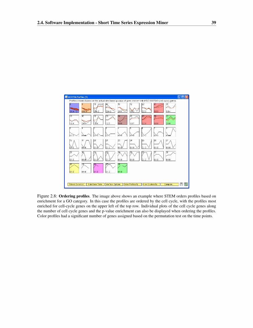
2.4. Software Implementation - Short Time Series Expression Miner 39
Figure 2.8: Ordering profiles. The image above shows an example where STEM orders profiles based onenrichment for a GO category. In this case the profiles are ordered by the cell cycle, with the profiles mostenriched for cell-cycle genes on the upper left of the top row. Individual plots of the cell cycle genes alongthe number of cell cycle genes and the p-value enrichment can also be displayed when ordering the profiles.Color profiles had a significant number of genes assigned based on the permutation test on the time points.
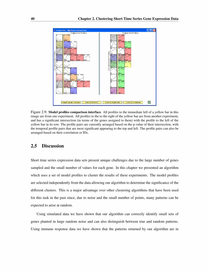
40 Chapter 2. Clustering Short Time Series Gene Expression Data
Figure 2.9: Model profiles comparison interface. All profiles to the immediate left of a yellow bar in thisimage are from one experiment. All profiles to the to the right of the yellow bar are from another experiment,and has a significant intersection (in terms of the genes assigned to them) with the profile to the left of theyellow bar in its row. The profile pairs are currently arranged based on the p-value of their intersection, withthe temporal profile pairs that are most significant appearing to the top and left. The profile pairs can also bearranged based on their correlation or IDs.
2.5 Discussion
Short time series expression data sets present unique challenges due to the large number of genes
sampled and the small number of values for each gene. In this chapter we presented an algorithm
which uses a set of model profiles to cluster the results of these experiments. The model profiles
are selected independently from the data allowing our algorithm to determine the significance of the
different clusters. This is a major advantage over other clustering algorithms that have been used
for this task in the past since, due to noise and the small number of points, many patterns can be
expected to arise at random.
Using simulated data we have shown that our algorithm can correctly identify small sets of
genes planted in large random noise and can also distinguish between true and random patterns.
Using immune response data we have shown that the patterns returned by our algorithm are in

2.5. Discussion 41
good agreement with the functional annotations of the associated sets of genes. Comparison to
k-means and CAGED indicated that by focusing on the set of significant profiles our algorithm
outperforms these algorithm resulting in a much more coherent set of genes. We have implemented
our clustering method along with additional features as part of the publicly available software, the
Short Time-series Expression Miner (STEM).
In this chapter our goals been largely descriptive, to identify clusters of genes having a statis-
tically significant temporal expression pattern. This leads naturally to the question as to whether
we can explain some of these observed significant temporal patterns in terms of the output of an
underlying dynamic regulatory network. In the next chapter we present a method to do so.


Chapter 3
Reconstructing Dynamic RegulatoryMaps∗
3.1 Introduction
In the previous chapter we observed that the expression level of genes in cells exhibit significant tem-
poral patterns in response to stimuli. A key challenge is to understand the dynamic programs that a
cell utilizes to respond to stimuli, which leads to these observed temporal patterns. These programs
activate regulatory networks controlled by transcription factors [60] and can involve the activation or
repression of a large number of genes [119]. Direct information about the gene targets of transcrip-
tion factors have been obtained through methods such as genome-wide Chromatin Immunoprecipi-
tation on chip (ChIP-chip) experiments and comparative genomics motif studies [59, 60, 192, 194].
Time series microarray expression experiments are a complementary source of data, providing dy-
namic information about the expression of thousands of genes that are activated or repressed in
response to stimuli such as environmental stress [48].
The method presented in the last chapter along with other methods that only use time series
data [8, 26, 34, 65, 80, 141, 159], although useful, only provide a partial view of the transcriptional
regulation process as they do not explicitly integrate information about transcription factor-gene
∗The content of this chapter is based on the paper [41].
43

44 Chapter 3. Reconstructing Dynamic Regulatory Maps
interactions. Most methods that integrate gene expression data with transcription factor-gene asso-
ciation data do so without explicitly taking into account the dynamic nature of biological systems.
A number of these methods combined a large number of expression data sets and motif data to
infer transcription modules [69, 135, 163]. Transcriptional modules are subsets of transcription fac-
tors and genes, such that genes in the same module tend to be similarly expressed and regulated
by the same transcription factors across a number of experimental conditions. Bar-Joseph et al [9]
integrated ChIP-chip data with expression data with a similar objective. Das et al [32] presented
a method that combined human expression data and motif information to identify active motifs,
combinations of motifs, and target genes under certain conditions. Although these prior methods
provided important insights and often used time series expression data sets, they did not take advan-
tage of the sequential ordering of time points in an expression experiment, essentially treating time
series and static expression data in the same way.
A few later methods proposed to integrate time series expression data with transcription factor-
gene association data while taking into account the ordering of experiments in time series data
sets. For instance, time series expression data were used to determine which genes were active
during certain time periods and then combined with ChIP-chip data using a trace-back algorithm to
identify active transcription factors during these time periods [103]. This method in effect identified
an ordered series of static regulatory graphs, but its direct connection with the dynamics of observed
gene expression patterns is less clear. Other methods have relied more heavily on individual gene
expression profile dynamics. For instance, Kundaje et al [86] forms independent clusters of genes
by using a joint probabilistic model for the dynamics of time series expression profiles of genes and
the motifs in their promoter regions. Others have integrated time series expression data with ChIP-
chip data to model the expression of individual genes [95] and interactions among transcription
factors [28] applying their techniques to model the cell cycle. Another method [18] used kinetic
equations based on the time series expression data to associate transcription factors with subsets of
genes across a subset of experimental conditions.
Our objective is different from that of these prior works. We present a computational method that

3.1. Introduction 45
integrates the time series expression data and transcription factor-gene association data to infer an
annotated global temporal regulatory map. This map describes the main transcriptional regulatory
events leading to the observed time series expression patterns and the factors controlling these events
during a cell’s response to stimuli. Our method focuses on bifurcation events. Bifurcation events
occur when sets of genes that have roughly the same expression level up until some time point
diverge (see Figure 3.1). Modeling expression patterns as results of a series of bifurcation events
is consistent with a multilayer hierarchical model of gene regulation previously suggested for some
organisms [7]. Our method attempts to both detect these bifurcation events and explain them in
terms of regulation by transcription factors. By focusing on detecting and explaining bifurcation
events, we can determine the time when transcription factors are exerting their influence. The
method also assigns genes to paths in the map based on their expression profiles and the transcription
factors that control them. The model we use to learn these maps is based on an instance of an Input-
Output Hidden Markov Model (IOHMM) [13], where the transcription factor-gene association data
is the input and the observed expression data are the output.
In this chapter we applied our method to study several stress responses in yeast. Our method
was able to automatically infer many aspects of the temporal responses, some of which were pre-
viously known whereas others were new predictions. These new predictions range from low-level
predictions regarding the timing of specific interactions to mechanistic predictions about the set of
transcription factors controlling recovery from stress to predictions related to phenotypic changes.
We have experimentally validated all types of these predictions leading to new roles for transcription
factors in controlling yeast response to stress. We also used our temporal maps to compare different
stress experiments and to identify a number of common control mechanisms. By using the time of
activation that our method assigned to transcription factors, we were able to identify cascades of
activators. Analysis of these cascades provides insights into the utilization of networks motifs and
condition-specific regulation in response to stress.

46 Chapter 3. Reconstructing Dynamic Regulatory Maps
3.2 Method - Dynamic Regulatory Events Miner (DREM)
Our method, termed the Dynamic Regulatory Events Miner (DREM), combines time series gene
expression data and static transcription factor-gene association data using an algorithm we extended
for learning Input-Output Hidden Markov Models (IOHMMs) [13]. IOHMMs are an extension
of Hidden Markov Models (HMMs). HMMs have been used in the past to model sequential data
including DNA and protein sequence data [36] and to cluster gene expression data [159]. In HMMs
as well as IOHMMs, hidden states are used to group genes by associating a cluster with each path
through the hidden states over time. In our application, each hidden state is associated with one
time point and represents a Gaussian distribution of the expression values for genes associated with
it (Figure 3.1). IOHMMs extend HMMs in that they allow for an additional input set that does
not necessarily change over time to control the transition probabilities of genes from state to state
(Figure 3.1). In our application, we use static transcription factor-gene association data (e.g. ChIP-
chip experiments or motif data) as this additional input information. Thus, our model encodes a
mapping from the transcription factor-gene association data to the observed temporal expression
values.
The set of hidden states and transitions between them leads to a structure for the global dynamic
map. We constrain the set of valid transitions between hidden states to enforce a tree structure
among the hidden states. This allows us to model bifurcation events, places in the time series where
subsets of genes that had similar expression values at prior time points diverge from each other.
The identification of these events using an IOHMM is biased to those splits for which different
sets of transcription factors regulate the divergent sets of genes. The algorithm searches over many
possible structures for the map, training the parameters associated with the structures, and then
scoring these structures to select the best one. Each gene is then assigned to a specific path in
the map based on its time series expression data and transcription factor-gene association data.
Following this assignment, we compute association scores for transcription factors and splits using
a hypergeometric distribution enrichment calculation. In Section 3.3.7 we discuss how to relax the
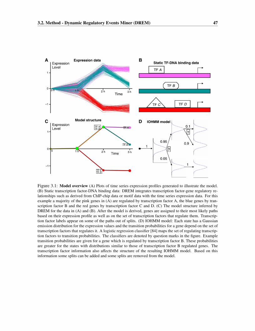
3.2. Method - Dynamic Regulatory Events Miner (DREM) 47
Figure 3.1: Model overview (A) Plots of time series expression profiles generated to illustrate the model.(B) Static transcription factor-DNA binding data: DREM integrates transcription factor-gene regulatory re-lationships such as derived from ChIP-chip data or motif data with the time series expression data. For thisexample a majority of the pink genes in (A) are regulated by transcription factor A, the blue genes by tran-scription factor B and the red genes by transcription factor C and D. (C) The model structure inferred byDREM for the data in (A) and (B). After the model is derived, genes are assigned to their most likely pathsbased on their expression profile as well as on the set of transcription factors that regulate them. Transcrip-tion factor labels appear on some of the paths out of splits. (D) IOHMM model: Each state has a Gaussianemission distribution for the expression values and the transition probabilities for a gene depend on the set oftranscription factors that regulates it. A logistic regression classifier [84] maps the set of regulating transcrip-tion factors to transition probabilities. The classifiers are denoted by question marks in the figure. Exampletransition probabilities are given for a gene which is regulated by transcription factor B. These probabilitiesare greater for the states with distributions similar to those of transcription factor B regulated genes. Thetranscription factor information also affects the structure of the resulting IOHMM model. Based on thisinformation some splits can be added and some splits are removed from the model.

48 Chapter 3. Reconstructing Dynamic Regulatory Maps
tree constraint to allow paths to converge during recovery periods. For the results in most of this
chapter, we only used the sampled time points; however, as we show in Section 3.3.8 one can also
use our model with interpolated values for time points that were not sampled. Finally, we note
that for the results in this chapter, we limited the analysis to binary splits although the method also
generalizes to higher order splits, for which we show an example in Chapter 4.
3.2.1 Probabilistic Model
The model DREM uses to integrate time series expression data with transcription factor-gene asso-
ciation data is based on a specific constrained instance of an Input-Output Hidden Markov Model
(IOHMM) [13] which we will denote as M (also see Figure 3.1).
Formally M is a tuple (H, E,Ψ,Θ, n, γ) where:
• n is a parameter for the number of discrete time points that M will be modeling.
• H is a set of hidden states. Each hidden state, h, is associated with a Gaussian output dis-
tribution, fh. Each hidden state h ∈ H is associated with one time point, denoted h.t, where
t ∈ {0, 1, ..., n − 1}.
• Θ is the set of parameters for the output distributions. For each hidden state h ∈ H there is
an element (µh, σh) ∈ Θ corresponding to the mean and standard deviation of the Gaussian
distribution fh.
• E contains the set of directed edges connecting hidden states of H, corresponding to valid
transitions among hidden states. If and only if (ha, hb) ∈ E then there is an edge from hidden
state ha to hidden state hb. Assuming paths are not allowed to be merged, the set of edges,
E, connecting the hidden states, H, are constrained to enforce a tree structure. Each hidden
state is constrained to have at most γ children. Formally we assume there is exactly one state
h ∈ H with h.t = 0 which forms the root of a tree. For any state a ∈ H with a.t < n − 1 there
must be at least one hidden state b ∈ H with (a, b) ∈ E satisfying a.t + 1 = b.t and no more

3.2. Method - Dynamic Regulatory Events Miner (DREM) 49
than γ such b. For any hidden state b ∈ H with b.t > 0 there must be exactly one state a such
that (a, b) ∈ E, additionally the relation a.t + 1 = b.t. If paths are allowed to be merged as a
post-processing step, then this last requirement is relaxed so that there may be more than one
such state a.
• Ψ contains the parameters controlling transition probabilities between hidden states. If a state
h ∈ H has two or more children, that is there are a, b ∈ H such that (h, a) ∈ E and (h, b) ∈ E
and a , b, then there is an element ψh ∈ Ψ. ψh is a vector of parameters for a logistic
regression classifier.
A logistic regression classifier [84] associated with state h is used to map a static transcription
factor-gene association input vector for a gene g, Ig, to transition probabilities among its children
states. For this chapter the jth element of Ig is 1 if transcription factor j is associated with regulating
gene g and 0 otherwise. In Chapter 4 we present an application where the jth element of Ig is 1 if
transcription factor j is associated with activating gene g, -1 if it is associated with repressing it, and
0 otherwise. We note that the model and algorithms below are the same for different representations
of the the transcription factor-gene association data, with the exception of the transcription factor
scoring as we will discuss in Section 3.2.4. We consider here binary logistic regression classifiers
corresponding to the case γ = 2, which is the setting of γ used for all results in this Chapter (see
Chapter 4 for results with γ = 3). If a gene g at time point (i − 1) is in a state h that has child states
h1 and h2, then the probability it is in state h1 at time point i can be written as
11 + e−ψh.b−
∑x(ψh.x)(Ig.x)
(3.1)
where the sum is over each element, Ig.x, of Ig and ψh.x is the corresponding element of ψ. ψh.b is
the intercept parameter of the logistic regression classifier.
As an example suppose our static input vector is based on four transcription factors Gcn4, Cbf1,

50 Chapter 3. Reconstructing Dynamic Regulatory Maps
Fhl1, and Sfp1. Suppose the static transcription factor-gene association input vector for gene g is
(Ig.Gcn4, Ig.Cbf1, Ig.Fhl1, Ig.Sfp1) = (1, 1, 0, 0). (3.2)
Further suppose that
ψh = (ψh.Gcn4, ψh.Cbf1, ψh.Fhl1, ψh.Sfp1, ψh.b) = (0.925, 0.607,−1.806,−2.018, 0.676) (3.3)
then for a gene g in state h the probability of transitioning to state h1 is
11 + e−ψh.b−
∑x(Ig.x)(ψh.x)
=1
1 + e−0.676−0.925×1−0.607×1+1.806×0+2.018×0 = 0.901 (3.4)
In contrast if Ig = (0, 0, 1, 1) then the probability of the gene transitioning to state h1 is 0.041. If γ is
greater than 2, then the logistic regression classifier naturally generalizes to the multi-class case [84]
(see also Chapter 4 for a discussion of multi-class logistic regression).
We note that requiring each hidden state to be associated with exactly one time point and the
constraints on transitions among the hidden states is specific to our application and not a general
property of an IOHMM. Also in a general IOHMM the output distribution can be dependant on the
input vector, and the input vector can be different at each time point, both of which are not the case
in this application.
Likelihood Function
Let og = (og(1), ..., og(n− 1)) be the log ratio expression values for gene g at time points 1 to (n− 1)
relative to a time point 0 control. Define Ht as the hidden state variable at time t. Denote the
transition probability for a gene g to transition to state hb at time point t given that it is in hidden
state ha at time point t as P(Ht = hb|Ht−1 = ha, Ig). This probability is defined as 0 if hb is not a
child of ha and 1 if hb is the only child of ha. If ha has two or more children then the transitions
are probabilistic and depend on the static input vector Ig. The mapping from static input vector

3.2. Method - Dynamic Regulatory Events Miner (DREM) 51
Ig to transition probabilities for a hidden state ha are determined by a trained logistic regression
classifier [84]. The log-likelihood function, l, for a set of genes G for the model M is
l(G|M) =∑g∈G
log∑q∈Q
n−1∏t=1
fq(t)(og(t))n−1∏t=1
P(Ht = q(t)|Ht−1 = q(t − 1), Ig) (3.5)
Q is the set of all paths of hidden states of length n starting from the root with non-zero probability.
For a path q ∈ Q, q(i) is the hidden state of the path at time point i. The first product is the product of
the output densities for the expression values and a given sequence of hidden states. If an expression
value is missing then its corresponding output density term is omitted from the product. The second
product is the product of transition probabilities for a given sequence of hidden states. The inner
sum is over all paths with non-zero probability. The outer sum is over all genes in G.
3.2.2 Parameter Learning
For a given H and E finding the setting of the parameters that globally optimizes Equation 3.5 above
is a non-convex optimization problem and in general cannot be guaranteed to be found. However
a local maximum can be found using a modification of the Baum-Welch training algorithm for a
regular Hidden Markov Model [36]. For our model above during each maximization step of the
Baum-Welch algorithm each logistic regression classifier is re-trained. The re-training algorithm
was based on the method of [84], which uses an L1 penalty on the coefficients of the classifier. The
use of the L1 penalty, the sum of the absolute value of each coefficient, promotes sparsity in terms of
the set of features used by the classifier. This is consistent with the expectation that a limited set of
transcription factors will be controlling each bifurcation. When training a classifier, for every gene
in the training set the classifier is given a weighted example of the gene in each child state. The
weight of the example is the probability of that gene going through that child based on the current
values of all the parameters in the model. For a state h with two children, h1 and h2, the parameters

52 Chapter 3. Reconstructing Dynamic Regulatory Maps
ψh are set to maximize:
∑g∈G
((wg,h1)(ln(P(Yg,h1 |ψh))) + (wg,h2)(ln(1 − P(Yg,h1 |ψh)))
)− λ
p∑j=1
|ψh. j| (3.6)
In the above expression λ is the regularization parameter that was set to 1. P(Yg,h1 |ψh) is determined
by Equation 3.1. In the penalty term on the right of the expression we index the elements of ψh
other than the intercept coefficient as ψh. j for j = 1, ..., p. wg,h1 and wg,h2 are the probabilities for
the time step (h.t + 1) that a gene with expression values og and input vector Ig would be in hidden
states h1 and h2 respectively. Formally we have for h, h1, and h2:
wg,h1 = P(Hh.t+1 = h1|og, Ig); wg,h2 = P(Hh.t+1 = h2|og, Ig) (3.7)
These probabilities are effectively computed when running the Baum-Welch algorithm [36].
3.2.3 Model Selection
Models that have more parameters available to them will be able to obtain higher likelihood values
in Equation 3.5, but also are more prone to overfitting the training data. We thus do not simply want
to select a model with the highest likelihood, but instead will consider two approaches to model
selection. One approach, which we will call the Train-Test approach, uses a portion of the data to
train the model, and the rest of the data as a test set. The likelihood of the model on the test set of
genes is used in selecting a model. In the second approach, Likelihood-Penalization, all the data is
used for training, but a penalty is placed on the number of states in the model. We discuss below in
more detail these two approaches to model selection. The results in this chapter were obtained using
the Train-Test approach, while in Chapter 4 we present results using the Likelihood-Penalization
approach.

3.2. Method - Dynamic Regulatory Events Miner (DREM) 53
Train-Test
To select a structure for the model, as determined by (H, E), a search starts from a single chain of
hidden states. The algorithm then performs a search over various structures. The algorithm splits
the set of genes into two sets, Gtrain and Gtest. Gtrain contains 75% of the genes and these genes
are used for training the parameters of structures under consideration. The remaining 25% of genes,
Gtest, are used for scoring the structures. The parameter training tries to find settings of Ψ and Θ that
maximize l(Gtrain|M) subject to the regularization on the elements of Ψ discussed above. The test set
score for a model, M, is l(Gtest|M). The search considers adding and deleting paths to the structure
while l(Gtest|M) increases. The search algorithm is summarized in the pseudocode in Figure 3.2.
After no more paths can be added or deleted from the model while improving the test set score, the
algorithm removes weakly supported paths that might be overfitting Gtest. To do this the algorithm
randomly re-splits the set of genes used for training and testing, generating a new test set test′. The
algorithm then deletes any path if the score for the retrained model with the path deleted, Mnew,
compared to old model, Mold, satisfies
(l(Gtest′ |Mnew) + κ|l(Gtest′ |Mnew)|) − l(Gtest′ |Mold) ≥ ζ (3.8)
where κ ≥ 0 and generally small and ζ ≤ 0. Here we set κ to 0.0015 and ζ = 0, increasing κ
or decreasing ζ would have the effect of removing more of the least supported splits. If multiple
paths satisfy the above property, then the path resulting in the largest score is selected first. Once a
path has been selected, Mnew becomes Mold and more paths can be deleted if they satisfy the above
property. A similar procedure is used to delay splits for which the split could have been placed one
time point later with no significant decrease on the score.
Optionally the algorithm can also merge paths which share a common split. An example of two
paths being merged is shown in Section 3.3.7. The criteria to accept a model with two paths merged
is the same as above except possibly with different choices of the parameters. To demonstrate a
merging in the Section 3.3.7 we set for the merging criteria κ to 0.0025 while ζ was still 0. If the

54 Chapter 3. Reconstructing Dynamic Regulatory Maps
algorithm decides to merge two paths, then the merged path can then be merged with another path
for which it now shares a split. For instance in the example of Figure 3.1 if the pink and blue paths
were merged at some later time point, then the merged pink and blue path could be merged with the
red path. We do not model scenarios where the red path merges with only one of the pink and blue
paths. Also we do not model scenarios where paths merge and then split again.
The algorithm then combines the train and test sets and retrains the model on the combined set
without changing the structure. Genes are then assigned to their most likely path using the Viterbi
algorithm [36]. Paths which have less than five genes assigned are removed. The splits and paths
are then scored for association with transcription factors (next subsection). It is important to note
that the map built will depend on the random training and test splits. Ideally then the algorithm
should be run several times with different random seeds generating different train and test splits of
the data.
Likelihood-Penalization
An alternative framework for model selection that directly uses all the data for model selection and
training the parameters, is to have a penalization term for model complexity. Our penalization term
was based on the number of states. The model which maximized the following expression was
selected:
l(G|M) − η|H| (3.9)
In the above η is a parameter which controls the trade-off between the likelihood score and the
number of states in the model. We choose here to base the regularization on the number of states
instead of the number of parameters, since it is possible to have a large number of logistic regression
parameters that have minimal effect on the likelihood.
The algorithm for learning the model is the same as for the Train-Test framework except splitting
the data into training and test sets is no longer necessary (steps 1 and 4) as well as the last deletion

3.2. Method - Dynamic Regulatory Events Miner (DREM) 55
Pseudocode for Train-Test Model Learning1. Partition gene set into a train set and test set.2. Initialize (H, E) to be a single chain of states, train chain, and compute test score.3. while test score improves do
a. (H′, E′)← (H, E)b. For each hidden state, h, that can have another child do
i. Temporarily add a single chain of hidden states from h to (H′, E′)ii. Train the temporary model from step 3.b.iiii. If the test set score for the model in 3.b.ii is the best found so far, then
let (H, E) be the model structure from step 3.b.iend forc. (H′, E′)← (H, E)d. For each hidden state, h, in H′, which has a sibling in H′ do
i. Temporarily remove h and all descendants from (H′, E′)ii. Train the temporary model from step 3.d.iiii. If the test set score is at least as good as the best so far, then
let (H, E) be the model structure from step 3.d.iend fore. If (H, E) was updated during 3.d.iii, then go to step 3c
end while4. Randomly resplit train and test data.5. Delete weakly supported paths.6. Delay appropriate splits.7. (Optional) Merge appropriate paths.8. Train parameters of model using all genes.9. Assign genes to paths using the Viterbi algorithm.10. Remove any path with fewer than 5 genes.
Figure 3.2: Above is the pseudocode that DREM uses to learn a model, using the Train-Test approach tomodel selection.

56 Chapter 3. Reconstructing Dynamic Regulatory Maps
step (step 5). Also instead of the test set score we use Equation 3.9 to score models.
One advantage of the Likelihood-Penalization model selection approach is that all genes are
used for selecting the model and training the parameter. Another advantage is an explicit preference
is placed for simpler models in terms of the number of states. In contrast for the Train-Test approach
in some cases it is possible that a simpler and a more complex model could have almost equivalent
likelihoods on both a training and test set of genes. On average though one should expect better
generalization using the Train-Test framework in terms of the likelihood on held-out genes as this is
more closely tied to the criteria the Train-Test uses to select models.
3.2.4 Transcription Factor Scoring
We first consider the case of binary transcription factor-gene association data, where a transcription
factor is either associated or not with regulating a gene. Consider a transcription factor f , a split S ,
and path A out of a split. Let nS be the total number of genes assigned to the path into the split. Let
nA be the total number of genes on path A out of the split. Let cS be the total number of genes into
the split associated with being regulated by transcription factor f , and let cA be the number of these
genes on path A. The score for transcription factor f for split S on path A is
min(cS ,nA)∑i=cA
(cSi
)(nS−cSnA−i
)(nSnA
) (3.10)
The lower the score the stronger the association of a transcription factor with a path out of a split.
This score is computed using the hypergeometric distribution and corresponds to the p-value a
Fisher’s exact test would compute for variable association for being regulated by f and on path A.
However the score does not represent a true p-value since the transcription factor information was
used to learn the model and assign genes to paths.
Overall enrichment for a transcription factor f along path A can be computed similarly, which
takes into account enrichment based on filtering and prior splits. Let R be the total number of genes
before filtering and cR be the total number of genes associated with being regulated by transcription

3.3. Results 57
Adr1 Arg80 Arg81 Aro80 Bas1 Cad1Cbf1 Cha4 Dal81 Dal82 Fhl1 Gat1Gcn4 Gcr2 Gln3 Hap4 Hap5 Leu3Met28 Met31 Met32 Met4 Mot3 Pho2Put3 Rap1 Rcs1 Rph1 Rtg1 Rtg3Sfp1 Sip4 Stp1 Uga3
Table 3.1: Transcription Factors with ChIP-chip data in Amino-Acid (AA) Starvation. Table of tran-scription factors with ChIP-chip data in AA starvation conditions from [60].
factor f . The overall score for transcription factor f on path A is
min(cR,nA)∑i=cA
(cRi
)(R−cRnA−i
)(RnA
) (3.11)
If we also have activator or repressor information in the input, then we compute two separate
scores, an activator and repressor score, for each transcription factor and path out of a split. The
activator score is the association of the transcription factor with its activated targets along the path,
while the repressor score is the association of the transcription factor with its repressed targets
along the path. These scores are computed as above except the counts for cA, cS , and cR are further
restricted to include only genes for which the transcription factor is an activator for the activator
score, or a repressor for the repressor score.
3.3 Results
3.3.1 A temporal map for amino-acid starvation response
To test the ability of the Dynamic Regulatory Events Miner (DREM) to learn dynamic maps from
time series and ChIP-chip data, we initially focused on the amino-acid (AA) starvation response
pathway in the yeast Saccharomyces cerevisiae. As AAs are the basic structural components of
proteins, yeast response to this stress by increasing AA synthesis and decreasing AA utilization is
critical for its survival. For this condition, we have detailed time series expression data [48] as well
as ChIP-chip experiments for 34 transcription factors [60] (Table 3.1). The time series expression

58 Chapter 3. Reconstructing Dynamic Regulatory Maps
Figure 3.3: Dynamic regulatory map and static network for yeast response to AA starvation. (A) Dy-namic map of yeast response to AA starvation using static input from condition-specific binding experimentsand time series expression data. Transcription factors with split score below 0.001 appear next to the splitthey regulate, in ranked order of scores. Nodes in the graph represent hidden states. The area of a nodeis proportional to the standard deviation of the expression of the genes assigned to that node. Green nodesrepresent split nodes. Many of the transcription factors were correctly assigned to the time points they areknown to regulate. For example, Gcn4, which is a known master regulator of AA starvation response, iscorrectly assigned to the first split. Many of the transcription factors assigned to the second split regulatespecific AA biosynthesis pathways. (B) Dynamic map of yeast response to AA starvation using input fromboth condition- and non-condition-specific ChIP-chip experiments. Several additional transcription factorsnot profiled with a condition-specific ChIP-chip experiment under the AA condition were determined to beparticipating in the response and recovery processes. These included Abf1, Swi4, Mbp1, and Ino4. In addi-tion to identifying these transcription factors as potential participants in the response, DREM also identifiestheir time of influence. (C) Static regulatory graph for AA starvation. Nodes correspond to genes or tran-scription factors. An edge implies that the transcription factor binds the gene with a p-value <0.005 in an AAstarvation ChIP-chip experiment. Blue edges represent interactions between transcription factors. Whereassome properties of the networks can be derived from the static representation, many of the dynamic aspectsof the system are lost when not using the time series data.

3.3. Results 59
data was sampled relative to an unstressed control at five time points, 0.5h, 1h, 2h, 4h, and 6h.
Genes were filtered if they had more than one missing data point or did not exhibit an absolute log
base two fold change of at least one for at least one time point, leaving 2029 of the 6152 genes
remaining. A transcription factor was associated with regulating a gene if the transcription factor
bound the promoter region of the gene with a p-value of <0.005. Figure 3.3A presents a temporal
map derived by DREM using these two data sets. This map contained 11 unique paths controlled
by a total of 15 transcription factors (using a transcription factor split association cutoff score of
0.001; see Section 3.2.4). In some cases, the same transcription factor appears multiple times on the
same path indicating multiple bifurcations with which the transcription factor is significantly asso-
ciated. As has been noted before, following AA starvation there is a massive transcription response
involving both activation and repression. Our algorithm assigned to the first bifurcation two sets
of transcription factors, Gcn4 and Cbf1 are associated with the genes that turn on upon starvation,
whereas Fhl1, Sfp1, and Rap1 are associated with the repressed genes (Figure 3.3A). These obser-
vations fit and expand current knowledge about this process. Gcn4 is indeed the master regulator
of the AA starvation response [62, 119], whereas Cbf1 has been previously associated with methio-
nine biosynthesis [6]. Our findings of Cbf1 association to the first bifurcation point suggest that it
has a broader role in the cellular response to AA starvation. Indeed, genes regulated by Cbf1 and
assigned to the higher path out of the first split were enriched not only for Gene Ontology (GO) [3]
categories like sulfur AA metabolism (p-value <10−9), which was previously noted [178], but also
for glutamate metabolism (p-value <4 × 10⁻⁶) and the more general AA metabolism category, with
a lower p-value (<7× 10⁻¹⁶). Gcn4 and Cbf1 are known to cooperate in the activation of the Met16
gene [123] and our finding of Gcn4 and Cbf1 as the two major activators in the AA response may
suggest that such cooperativity is much more common. Indeed, we observe a significant overlap
in genes bound by both Gcn4 and Cbf1 (p-value <4 × 10⁻⁸). Many of the transcription factors
assigned to the second time point (secondary transcription factors) are known regulators of specific
AA biosynthesis pathways, including Met4 as well as Arg81, Met32, and Dal82. Using GO, we
determined that the set of genes assigned to the highest path after the first time point was enriched

60 Chapter 3. Reconstructing Dynamic Regulatory Maps
Arg81 Cbf1 Dal82 Fhl1 Gcn4Gln3 Hap5 Met31 Met32 Met4Met4 Rap1 Rtg3 Sfp1 Stp1
Table 3.2: Table of transcription factors with AA starvation ChIP-chip data from [60] appearing on the mapin Figure 3.3B.
Abf1 Ino4 Mbp1Swi4 Yap7
Table 3.3: Table of transcription factors without AA starvation ChIP-chip data from [60] appearing on themap in Figure 3.3B. The increased binding activity of Ino4 in the response to AA starvation was confirmedwith new ChIP-chip data.
for AA metabolism (p-value <9× 10−39) and subcategories such as glutamate biosynthesis (p-value
<10−13), sulfur AA metabolism (p-value <6 × 10⁻¹⁰), methionine metabolism (p-value <2 × 10⁻⁹),
and arginine metabolism (p-value <4× 10⁻⁹). Two other transcription factors assigned to this point,
Rtg3 and Gln3, are activated upon starvation in a TOR pathway-related manner [31].
The set of genes assigned to the repressed path out of the first split is highly enriched in cate-
gories such as ribosome biogenesis and assembly (p-value <10−91) and ribosome (p-value <10−83)
consistent with what has been observed before for AA starvation response [48]. A majority of the
ribosomal genes were determined to be bound by the ribosomal transcription factors Rap1, Fhl1, or
Sfp1. It has been previously noted that Rap1 and Fhl1 remain bound to the promoter regions of ribo-
somal genes under environmental stress [151, 185]. An additional transcription factor, Ifh1, which
has recently been implicated in having an important role in controlling the expression of ribosomal
genes under stress [151, 185] was not part of the set of transcription factors for which a ChIP-chip
experiment was performed in AA starvation conditions.
3.3.2 Extending condition-specific dynamic maps using general binding data
Although the map derived by DREM provided explanations for several bifurcation points, others
could not be explained using the limited set of transcription factors with ChIP-chip data under the
AA starvation condition. We have hypothesized that some of these points could be explained by

3.3. Results 61
transcription factors, which were previously not known to be involved in this process and so were
not originally profiled with ChIP-chip experiments in AA starvation conditions. To test this, we
have employed DREM again, this time augmenting the static input data with an additional 75 tran-
scription factors profiled with ChIP-chip experiments in other conditions in yeast, primarily yeast
complete growing media (YPD) [60]. To reduce false positives in using ChIP-chip data when asso-
ciating a transcription factor with regulating a gene, we followed a version of the regulatory code
of [60] that required in addition to a ChIP-chip binding p-value of <0.005 in at least one condi-
tion, an evolutionarily conserved motif in at least two other yeast species among the yeast species
considered. The map derived from this additional data (Figure 3.3B) contained new transcription
factors that explained a number of temporal events (Tables 3.2 and 3.3). Some of these transcription
factors were added to previously annotated time points. For instance, Yap7 was assigned to the
set of secondary transcription factors on the top split. Abf1 was assigned to the first split and was
determined to control genes that were downregulated early on. This agrees with previous studies
that implicated Abf1 in being involved in regulating the ribosome [33, 136]. Two G1 cell-cycle
activators, Swi4 and Mbp1, now appear on a split starting at the 2h point on the recovery path. This
path was enriched for genes previously shown to be cell cycle regulated [174] (p-value <9 × 10⁻⁶),
where enrichment was based on all genes going into the split. Another factor, Ino4, which has been
implicated in phospholipid biosynthesis [82] and more recently has been suggested to be a global
regulator of gene expression [156, 192], was determined to be activating genes starting around the
2h time point. Several of the genes in the path that DREM determined to be controlled by Ino4
were known lipid metabolism genes (GO p-value <6× 10⁻⁵). The induction of Ino4-regulated lipid
biosynthesis genes may be connected to the immediate need of membrane used for the autophagocy-
tosis process. This process is utilized by yeast in order to regulate the equilibrium between proteins
and the diminishing set of AAs due to the starvation condition [133].

62 Chapter 3. Reconstructing Dynamic Regulatory Maps
3.3.3 Validating interactions and mechanistic predictions
The temporal map derived by DREM suggests that Ino4 is activating genes as part of a recovery
mechanism several hours after AA starvation. However, Ino4 had previously only been profiled
with a ChIP-chip experiment in YPD media [60]. To validate the prediction of Ino4’s role in AA
starvation conditions, we first carried out ChIP-PCR experiments in which we checked the in vivo
association of the Ino4 protein to several of its targets. We selected four of the genes bound by Ino4
in the ChIP-chip experiment in YPD media with a p-value <0.005 that were assigned to the path
most significantly controlled by Ino4 (brown path in Figure 3.3B and genes in Figure 3.4A). We
compared the occupancy of Ino4 in the promoter of these genes in synthetic complete+D-glucose
(SCD) media and 4h after AA starvation (method details for the biological experiments can be found
in [41]). As Figure 3.4B shows, for three of the four genes, the occupancy rate of Ino4 at 4h after
AA starvation is at least twice its rate in SCD media, suggesting that Ino4 indeed plays a role in
regulating these genes during AA starvation, as predicted by DREM. To further characterize Ino4’s
increased activity in regulating genes in AA starvation, we carried out a genome-wide binding
experiment for Ino4 in SCD conditions and at 4h into AA starvation. As Figure 3.4C shows, Ino4
binds to many more genes in AA starvation conditions as compared to its binding in SCD (125
more genes at a p-value <0.001 in at least one repeat and 66 more genes at a p-value <0.005; see
also Table 3.5). Of the 207 genes bound by Ino4 at a p-value <0.005, 34 were among the 422
genes assigned to the path that DREM identified as most associated with Ino4 (p-value <2 × 10⁻⁶).
Furthermore, as the plots show Figure 3.4D almost all of the genes assigned to this path that are
bound by Ino4 in either AA starvation, SCD media, or both, are more significantly bound in AA
starvation conditions.
3.3.4 Temporal maps for the regulation of stress response in yeast
We next combined condition- and non-condition-specific binding data and used DREM to construct
temporal regulatory maps for a number of other stress conditions for which time series expression
data was available in [48]. These conditions include heat shock (Figure 3.5A), DTT (Figure 3.15),
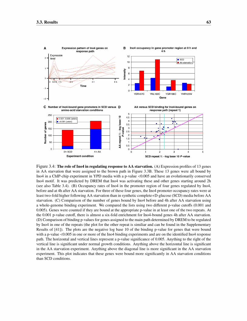
3.3. Results 63
Figure 3.4: The role of Ino4 in regulating response to AA starvation. (A) Expression profiles of 13 genesin AA starvation that were assigned to the brown path in Figure 3.3B. These 13 genes were all bound byIno4 in a ChIP-chip experiment in YPD media with a p-value <0.005 and have an evolutionarily conservedIno4 motif. It was predicted by DREM that Ino4 was activating these and other genes starting around 2h(see also Table 3.4). (B) Occupancy rates of Ino4 in the promoter region of four genes regulated by Ino4,before and at 4h after AA starvation. For three of these four genes, the Ino4 promoter occupancy rates were atleast two-fold higher following AA starvation than in synthetic complete+D-glucose (SCD) media before AAstarvation. (C) Comparison of the number of genes bound by Ino4 before and 4h after AA starvation usinga whole-genome binding experiment. We compared the lists using two different p-value cutoffs (0.001 and0.005). Genes were counted if they are bound at the appropriate p-value in at least one of the two repeats. Atthe 0.001 p-value cutoff, there is almost a six-fold enrichment for Ino4-bound genes 4h after AA starvation.(D) Comparison of binding p-values for genes assigned to the main path determined by DREM to be regulatedby Ino4 in one of the repeats (the plot for the other repeat is similiar and can be found in the SupplementaryResults of [41]). The plots are the negative log base 10 of the binding p-value for genes that were boundwith a p-value <0.005 in one or more of the Ino4 binding experiments and are on the identified Ino4 responsepath. The horizontal and vertical lines represent a p-value significance of 0.005. Anything to the right of thevertical line is significant under normal growth conditions. Anything above the horizontal line is significantin the AA starvation experiment. Anything above the diagonal line is more significant in the AA starvationexperiment. This plot indicates that these genes were bound more significantly in AA starvation conditionsthan SCD conditions.

64 Chapter 3. Reconstructing Dynamic Regulatory Maps
YDR497C YER026C YER092W YGR196C YHR123WYIL119C YJL048C YJL141C YJL167WYNL169C YNL180C YOR316C YOR317W
Table 3.4: Ino4 Regulated Genes Based on the Input that are also on the Response Path. 13 Ino4predicted regulated genes that appear on the main Ino4 response path. These genes are all bound in YPDmedia by Ino4 at a p-value <0.005 and have a conserved motif for Ino4.
Ino4 Intergenic region Genes Intergenic region Genesbinding experiment p-val <0.001 p-val <0.001 p-val <0.005 p-val <0.005
SCD repeat 1 16 21 88 114AA repeat 1 68 89 122 153
Increase in AA repeat 1 325% 324% 39% 34%SCD repeat 2 5 6 78 94AA repeat 2 46 59 109 147
Increase in AA repeat 2 820% 883% 40% 56%
Table 3.5: Experimental results for Ino4 binding in amino-acid starvation. Summary of binding in Ino4genome-wide ChIP-chip binding experiments. The table gives the number of intergenic regions bound andthe number of associated genes at both the 0.001 and 0.005 p-value significance levels for two repeats. Onlyintergenic regions with assigned genes are included in the intergenic region counts. The table also givesthe percentage increase in AA conditions compared to that in SCD media, which is the condition beforestarvation. These percentages indicate the increased activity of Ino4 at 4h into AA starvation.
and hydrogen peroxide (Figure 3.6) (see also Supporting Results of [41] for a discussion of DREM
with cold shock). All of these had time series expression data available [48]. The number of
transcription factors for which we used condition-specific binding data in the input varied from 28
for hydrogen peroxide one for heat shock, and none for DTT. All condition-specific binding data
were obtained from [60] (using a p-value of <0.005) except the heat-shock binding data, which
were obtained from the list of Hsf1 targets determined from [59]. As in the AA starvation example
above, we extended the input to include non-condition-specific binding data post-processed using
motif data from [60]. Again, DREM was able to reconstruct a number of known cascades and
suggest new regulatory roles.
For example, for heat shock, Hsf1 was identified as a ‘master’ regulator controlling the initial
activation response, which is consistent with previous studies [19]. Msn2- and Msn4-regulated
genes were also over-represented on the highest expressed paths of the heat-shock model. The set
of genes assigned to the path that was still increasing at 10 min was over-enriched for GO categories

3.3. Results 65
Figure 3.5: Cell-cycle recovery from stress. (A) Dynamic regulatory map derived for heat shock. As partof the recovery process, several genes regulated by Swi4, Swi6, Mbp1, and Fkh2 increase their expressionlevel, reaching a level higher than their original (nontreated) values. Many of these genes are G1 genes (p-value <4 × 10⁻²⁰ based on a set of 300 G1 genes from [174]). (B) Expression profiles of genes assignedto the bifurcation event at the 40 min time point. Blue profiles represent genes assigned to the upper pathof this bifurcation node. This path was controlled by the above cell-cycle transcription factors. Note thatthe expression of many of these genes rises above their initial expression value starting at the 60 min timepoint. (C) Budding index before and after heat shock. Cells are initially arrested and as predicted by DREMthe percentage of G1 cells peaks starting at the 60 min time point. Following that peak, cells resume theircell-cycle activity in a more synchronized manner.

66 Chapter 3. Reconstructing Dynamic Regulatory Maps
such as carbohydrate metabolism (p-value <10−14), response to stress (p-value <3 × 10⁻⁹), and
protein folding (p-value <6 × 10⁻⁷). All 15 of the protein folding genes assigned to this path were
also bound by Hsf1.
Figure 3.6: Dynamic Map of Hydrogen Peroxide Response. Temporal map derived by DREM for theHydrogen Peroxide stress experiment of [48]. Transcription factor labels for a path out of a split appear iftheir split score is less than 0.001 (see Section 3.2.4) and are ranked order by most significant score. The topof a box of transcription factor labels is aligned with the top of the circle representing the next state on thepath out of the split. The area of a circle is proportional to the standard deviation of the Gaussian distributionof the associated state.
For peroxide, Yap1 and Skn7 were two of the transcription factors correctly assigned to activated
paths in the first bifurcation point, consistent with a previous report [88]. Other transcription factors
associated with regulating initially activated genes include Yap7, Rpn4, Msn2, Msn4, Gcn4, Aft2,
and Put3. The genes on the initially activated path were enriched for GO categories such as aldehyde
metabolism (p-value <2 × 10⁻⁹) and response to oxidative stress (p-value <6 × 10⁻⁹). Along the
repressed paths are cell-cycle transcription factors Mcm1, Sum1, Swi5, and Swi6 and ribosomal
transcription factors Fhl1 and Rap1, all of which were detected without hydrogen peroxide binding
data (Supporting Results of [41]).
Using these temporal stress response maps, we looked for common mechanisms employed by
yeast in response to stress.

3.3. Results 67
Repressed pathways
While the identity of many of the activators varied depending on the stress condition, we observed
two pathways that were generally repressed under the stress conditions we looked at. The first
pathway showed a similar pattern of repression and recovery in all of the reconstructed temporal
regulatory maps that we present here. This pathway included the ribosomal genes and their pri-
mary transcription factors (Rap1, Sfp1, and Fhl1). These genes are repressed steeply and quickly.
However, these genes also recovered quickly approaching their pre-treatment levels.
Another common repressed pathway that was observed in AA starvation and heat shock was a
pathway controlled by Swi4, Swi6, and Mbp1. This pathway primarily contained cell-cycle genes.
For example, in the heat-shock pathway, there was a particularly strong enrichment for G1 cell-
cycle genes [174] (p-value <4 × 10⁻²⁰). In comparison to the ribosomal genes, cell-cycle genes
were repressed at a slower rate and to a less significant level (Supporting Results of [41]). However,
when they recover, they were expressed at a higher level than their initial (time point 0) value (Fig-
ure 3.5B). A possible explanation to the slow repression of the cell-cycle genes, which is followed
by a strong activation, is that what we are actually seeing is the well-documented stress-related cell-
cycle arrest. In an unsynchronized culture, the downregulation of G1 genes should be gradual as it
takes time until all cells leave the G1 phase. On the other hand, in the recovery stage, the culture
is relatively synchronized and therefore the G1 genes reach higher levels than in unsynchronized
culture. To test the prediction that this pathway in heat shock indeed represents differences in the
cell-cycle phase distribution, we counted the budding index of cells following heat shock. As Fig-
ure 3.5C shows, 20-40 min after heat shock, cells enter S-phase arrest (increase in the fraction of
cells with small buds). Later, at around 50 min, the cell cycle resumes. However, the stress causes
partial synchronization of the cells (note the higher percentage of cells in G1 60 min after heat shock
compared to unsynchronized cells). These results agree well with the predictions made by DREM.
The increase in the expression values of the Swi4-Swi6 controlled path at the 60 min time point is
the result of the increase of synchronization. Following this, cells become partially synchronized,
at least for the next 120 min.
68 Chapter 3. Reconstructing Dynamic Regulatory Maps
Master regulators and condition-specific regulation in response to stress
Although the identity of the activators varied, a few activators were identified to have a much more
significant control of the initial change in expression levels in response to AA starvation (Gcn4,
Cbf1, Rap1, Fhl1, and Sfp1) and heat shock (Hsf1, Msn2/4, and Skn7). This can be seen most
clearly in the AA map where the majority of the activators in these conditions were activating genes
in later time points. This type of response can result from cells that constitutively express a small
number of master regulators so that they can react quickly to stress whereas the later transcription
factors are only expressed as part of the response process. This is consistent with previous stud-
ies. For example, Msn2 and Msn4 are regulated at the level of nuclear exclusion [52], Cbf1 also
already exists in the cell before starvation and its transcript level is not affected by methionine star-
vation [113], and Gcn4 and Hsf1 are found in association to a subset of their target gene promoters
even before stress [59, 60]. These differences are also apparent in the initial expression levels of
the regulators. As Figure 3.7C shows, during the first two time points, where their impact on the
genes they regulate is the highest, master regulators do not drastically change their own expres-
sion when compared with pretreatment levels. In contrast, the expression levels of most secondary
transcription factors increase, indicating that many are transcriptionally regulated.
To further study this point, we looked at the condition-specific regulation activities of transcrip-
tion factors in AA starvation and heat shock by dividing the transcription factors into two groups:
the first contained transcription factors that were determined to control the initial response and the
second contained secondary transcription factors assigned to a second split point. We compared
the binding targets of these transcription factors under YPD media and in the condition that they
regulate. As part of the response to stress, several yeast transcription factors begin to regulate genes
that were not regulated by them in YPD media [9, 103]. As can be seen in Figure 3.7A, regulators
controlling the first bifurcation point (master regulators) showed a much larger overlap in the set of
genes bound in stress and YPD media compared to the transcription factors regulating genes at later
time points (secondary regulators). Whereas six of the eight transcription factors assigned to a first
point had more than 20% overlap between condition-specific and YPD media binding data, and four

3.3. Results 69
Figure 3.7: Distribution of binding overlap between YPD media and stress condition for differentsets of transcription factors. We group transcription factors into two sets. The first subset contains thetranscription factors assigned to first split points in AA starvation or heat that were profiled with a ChIP-chipexperiment in the condition (8, primary transcription factors Cbf1, Gcn4, Fhl1, Rap1, and Sfp1 from AAstarvation in [60] and for heat Msn2 and Skn7 from [60] and Hsf1 from [59]) and the secondary transcriptionfactors assigned to second split point profiled with a ChIP-chip experiment in the condition (8, secondarytranscription factors Arg81, Dal82, Gln3, Hap5, Met32, Met4, Rtg3, and Stp1 from AA starvation in [60]).(A) Percent overlap for each of these two sets when binding (under both stress and YPD media conditions) isdetermined using a 0.005 p-value cutoff. Note the difference between the distribution of overlap for primaryand other transcription factors. Whereas the majority of transcription factors display a big difference in the setbound genes under stress and YPD media, many primary transcription factors bind to a large percentage ofstress-regulated genes in YPD media as well. This difference is even bigger in (B) where we plot the overlapfor the top 100 genes (ordered by their binding p-values) in each condition. Whereas most transcriptionfactors (and most secondary transcription factors) drastically alter the subset of genes they regulate understress, half of the primary factors bind to more than 50% of the same genes in both conditions. Althoughthe binding strength may be different under stress, these results indicate that many of the primary pathwaysare maintained, in low levels, under YPD media as well. (C) Average expression levels for primary andsecondary factors for the first two time points in the AA starvation and heat-shock experiments. Whereas theaverage expression levels for the secondary factors are much higher when compared to their untreated levels,the levels for the primary factors do not change significantly between the two conditions.

70 Chapter 3. Reconstructing Dynamic Regulatory Maps
had more than 50% overlap, six of the eight transcription factors first appearing at a second split had
less than a 20% overlap and none had more than 50% overlap (see also Supporting Results of [41]).
These results hold even if we ignore the actual p-values and focus on the list of 100 top bound genes
in each condition (Figure 3.7B). Again, these differences indicate that, at least for some types of
stress, cells maintain the ability to quickly activate the initial response pathways.
In addition to differences in the condition-specific activity between master and secondary reg-
ulators, we have also observed differences in the utilization of different network motifs. As Fig-
ures 3.8 and 3.9 show for the AA condition, genes bound by master regulators that are activators in
a feed forward loop (FFL) displayed consistently higher expression levels when compared to genes
regulated by the same transcription factors in a multiple input (MI) or single input (SI) motifs. In
contrast, for many secondary transcription factors, we have not observed a large difference between
the expression levels of FFL-controlled genes and genes controlled by the other two network motifs.
The ability of master regulators to utilize FFLs by consistently expressing some of the genes at a
higher level during a response may help cells fine-tune their response to various stresses. Indeed,
whereas 45% of the genes bound by Gcn4 in an FFL are known AA biosynthesis genes (based on
GO), only 21 and 13% of the genes bound in an MI or an SI, respectively, are assigned to this cate-
gory. Thus, although many genes are activated initially, only a few of them will remain expressed at
a high level in a later point as their expression requires the additional binding of a secondary factor.
In this way, an FFL serves as a filtering motif, removing signals that were erroneously activated and
maintaining those that are required for the actual response pathway [104].
3.3.5 Determining the activation time of regulators
As the results above indicate, most transcription factors that are activated during stress either change
or expand the set of genes they regulate. To identify these new sets, ChIP-chip experiments are often
used to determine the roles of several transcription factors in various response pathways [9, 60, 192].
However, even when transcription factors are known, or suspected, to be involved in such pathway,
the actual time in which they are activated may vary. Master regulators are activated early on,

3.3. Results 71
Figure 3.8: Network Motif Expression Comparison in Amino Acid Starvation Response. (a) NetworkMotif diagrams for Multiple Input (MI), Feed Forward Loop (FFL), and Single Input (SI). (b) Comparisonof mean expression patterns of genes regulated in a FFL, MI and not an FFL, or SI for Cbf1, Gcn4, Arg80,and Dal81. Arg and Met complex transcription factors were considered to regulate genes even if not boundthemselves if another transcription factor in its complex bound the gene. Only transcription factor pairs withsignificant intersection of target genes (number of genes ≥ 5 and intersection p-value <0.005) were includedas active FFLs.
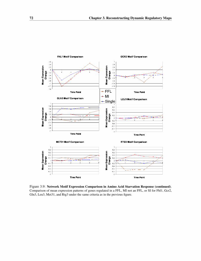
72 Chapter 3. Reconstructing Dynamic Regulatory Maps
Figure 3.9: Network Motif Expression Comparison in Amino Acid Starvation Response (continued).Comparison of mean expression patterns of genes regulated in a FFL, MI not an FFL, or SI for Fhl1, Gcr2,Gln3, Leu3, Met31, and Rtg3 under the same criteria as in the previous figure.

3.3. Results 73
Figure 3.10: Dynamic Map of MMS Response. Temporal map derived by DREM for the MMS experimentof [47]. (a) Portion of map above the x-axis. (b) Portion of map below the x-axis. Those transcription factorlabels without ‘MMS’ are based on ChIP-chip experiments in YPD media, and those with the ‘MMS’ labelare based on ChIP-chip experiments in the MMS condition. Transcription factor labels appear if their splitassociation score for the path is less than 0.001 (see Section 3.2.4) and are ranked order by most significantscore. The top of a box of transcription factor labels is aligned with the top of the circle representing the nextstate on the path out of the split. We see in (a) that Gcn4 is the top ranked transcription factor on the highestactivated path between 5 and 15 min, but then among initially activated genes it is most associated with arepressed path after 15 min.
Gcn4 Binding Intergenic Region Genes Intergenic Region GenesExperiment p-val <0.001 p-val <0.001 p-val <0.005 p-val <0.005
YPD Repeat 1 21 26 34 44MMS 15 min Repeat 1 106 155 151 221
YPD Repeat 2 23 26 38 45MMS 15 min Repeat 2 112 159 165 235MMS 60 min Repeat 2 107 154 150 212
Table 3.6: Gcn4 Binding in MMS Experimental Results. Summary of binding in Gcn4 genomewide binding experiments. Table gives number of intergenic regions bound and number of associ-ated genes at both the 0.001 and 0.005 significance levels for two repeats. Only intergenic regionswith assigned genes are included in the intergenic region counts.

74 Chapter 3. Reconstructing Dynamic Regulatory Maps
Figure 3.11: Comparison of binding p-values for Gcn4 in the MMS condition at 15 and 60 min. Pointsabove the diagonal correspond to genes that were bound more significantly at 15 min than at 60 min. As canbe seen from the plot, a substantial majority of genes were bound more significantly at 15 min than at 60min. Points to the right of the vertical had a p-value <0.005 in MMS at 60 min, whereas points above thehorizontal line had a p-value <0.005 in MMS at 15 min.
whereas secondary regulators are activated later. The ability of DREM to determine a time point
for carrying out such experiment can help in accurately recovering the role a factor plays in a
response pathway. To study this, we have looked at the activation of Gcn4 as part of the response
to methyl-methanesulfonate (MMS) stress in yeast. In a previous study, it was determined, using
an experiment 60 min after the induction of stress, that Gcn4 did not expand the set of genes it
regulates when compared to the set it regulates in YPD media [192]. We used DREM to reconstruct
a dynamic map for this system (Figure 3.10). As input we used time series gene expression data
for methyl-methanesulfonate (MMS) obtained from [47], which was sampled at 0, 5, 15, 30, 45,
60, 90, and 120 minutes into the response. Genes were filtered if they had more than one missing
data point, or their expression change did not exceed an absolute value of 0.6 at any time point
leaving 2227 genes. The ChIP-chip data was obtained from [192] and consisted of 30 transcription
factors from 60 min into the MMS condition, and an additional 105 transcription factors profiled
in YPD media. The YPD media ChIP-chip data was based on data originally published in [89].
The static transcription factor-gene association input vector for a gene had 135 elements. For 105

3.3. Results 75
of the elements, corresponding to the 105 YPD media ChIP-chip experiments, a ‘1’ was encoded
if the gene was bound by the transcription factor in the ChIP-chip experiment at a p-value <0.005
otherwise a ‘0’ was encoded. No motif constraints were used here. For the remaining 30 elements,
corresponding to the 30 MMS ChIP-chip experiments, a ‘1’ was encoded if the gene was bound
by the transcription factor in the ChIP-chip binding data at a p-value <0.005, otherwise a ‘0’ was
encoded. Some of the transcription factors appeared twice in the input, once based on their YPD
media ChIP-chip data and the other time based on their MMS ChIP-chip data.
The DREM map inferred for this condition made two predictions about Gcn4: (1) that Gcn4
was expanding the set of genes it regulates at the 15 min time point when compared to YPD media
and (2) that Gcn4 binding would likely be less intense at 60 min as the expression of the main Gcn4-
controlled paths decreased at that time point. To test whether the temporal predictions of DREM
were correct, we carried out genome-wide binding experiments at three time points: 0 (YPD media),
15, and 60 min. As predicted by DREM, we found a large expansion in the set of genes regulated
by Gcn4 at the 15 min time point. Whereas 45 genes were bound by Gcn4 in YPD media (using a
0.005 p-value cutoff), 235 genes were bound at the 15 min time point and a smaller number (212
genes) at the 60 min time point (Table 3.6). In addition, for the vast majority of Gcn4-bound genes,
the binding p-value was more significant at the 15 min time point when compared to the 60 min
point, indicating that Gcn4 is indeed more active earlier in the response as predicted by DREM
(Figure 3.11D). We note that our results, indicating that Gcn4 is expanding the set it regulates even
at the 60 min time point, differ from previously reported results [192]. There could be several
reasons for this discrepancy, the most likely source is the noise associated with any high-throughput
experiment. However, the fact that our 60 min results agree well with the 15 min results, with
the expression data, and with the findings of a previous study [119] indicates that Gcn4 is indeed
activating genes as part of the MMS-response pathway.

76 Chapter 3. Reconstructing Dynamic Regulatory Maps
3.3.6 Verifying the advantage of integrating time series expression and ChIP-chip
data
To verify the advantage gained from integrating time series expression data and ChIP-chip data, we
tested whether either data alone could have reproduced results similar to those obtained when com-
bining them. First, we generated a randomized version of the AA ChIP-chip data by randomizing
the genes each transcription factor was bound to while holding the number of genes bound by each
transcription factor fixed. We then applied DREM to this randomized ChIP-chip data and the origi-
nal AA gene expression data. This procedure resulted in maps that had no, or very few, transcription
factor labels (Figure 3.12). Specifically, we found that activators that were determined to be ‘mas-
ter’ regulators using the real binding data were not assigned to the first split using the randomized
values and most of the AA biosynthesis regulators were not assigned to any of the splits. Second,
we applied an HMM model to the time series data without using ChIP-chip while still enforcing
the same tree structure requirements on the hidden states. To compare the HMM model with the
IOHMM model of Figure 3.3B, we did use the ChIP-chip data as a post-processing step to score the
transcription factors at each split. We found that most of the relevant transcription factors were sub-
stantially more significant with an IOHMM than with an HMM (Figure 3.13). To further validate
that the grouping of genes were more biologically meaningful when using the IOHMM compared
to an HMM, we performed GO enrichment comparisons and found more GO categories to be en-
riched in an IOHMM model (Figure 3.14). Combined, these results demonstrate the importance of
the ChIP-chip data for determining an accurate regulation model. To demonstrate the importance of
the time series data for inferring regulatory models, as opposed to ChIP-chip data alone, we present
a regulation graph in Figure 3.3C. This graph uses only the ChIP-chip AA-binding data. Although
one can rank transcription factors based on the number of genes they regulate, it is clear from the
figure that it would be very hard to infer the dynamics of the response process from the ChIP-chip
data alone.

3.3. Results 77
Figure 3.12: Dynamic Maps for Amino Acid Starvation Response with Randomized ChIP-chip Input.Three maps learned by DREM for AA starvation time series and randomized AA ChIP-chip binding data.In the randomization procedure the number of genes passing filter that a transcription factor was associatedwith in the real input was held fixed, but the set of genes it bound to was otherwise selected randomly. Therandomization was applied independently for each transcription factor. The entire randomization procedurewas repeated three times to generate three different randomized input data sets. The above image shows themaps inferred by DREM using these randomized input data sets with transcription factors appearing if theirsplit score was lower than 0.001 as in Figure 3.3A. In two cases there were no transcription factor labelsappearing on the map, while in the third case there was three unique transcription factors (Gcn4, Rap1, andCha4) appearing (one transcription factor appeared at two splits). In contrast in the map of Figure 3.3A thereare 15 unique transcription factors appearing on the map. In addition, the temporal assignments differedsignificantly between the true and randomized data. While the true ChIP-chip data agreed well with theexpression data in terms of the roles known transcription factors play in regulating this response, there wasno such agreement for the randomized data. This demonstrates the compatibility of the ChIP-chip data andthe time series data.

78 Chapter 3. Reconstructing Dynamic Regulatory Maps
Figure 3.13: Comparison of transcription factor scores in an IOHMM vs. HMM. (Top) Map learnedwith an HMM that only uses the AA time series expression as input, and post-processing labeling the splitsbased on the same set of 109 transcription factor used for Figure 3.3B. Compared to Figure 3.3B there arefewer relevant transcription transcription factor assigned, especially for later time points. (Bottom Left) Therank order of the log-ratio of the minimum split score for a transcription factor anywhere in the model usingan IOHMM compared to an HMM. The scores are derived for each transcription factor based on the medianof 21 runs using different initial random seeds for the train-test data split. The scores above 0 imply a strongerassociation for a split path in an IOHMM and those below 0 represent a stronger association in an HMM.(Bottom Right) Similarly the rank order of the log-ratio of the minimum overall score for a transcriptionfactor anywhere in the model using an IOHMM compared to a regular HMM. The graph shows for almost alltranscription factors its minimum split and overall score is either better or about the same in an IOHMM ascompared to an HMM. This is especially true for most of the top 15 factors which DREM determined to beassociated with this response.

3.3. Results 79
Figure 3.14: Comparison of GO enrichment in an IOHMM vs. HMM. A comparison of level 3 GeneOntology (GO) categories significantly enriched in paths of an IOHMM or a HMM using the same data asin Figure 3.13. The comparison is restricted to GO categories with a minimum p-value <0.001 in eithermodel. The p-value for each category was computed based on the median of 21 runs with different initialrandom seeds for the train-test data split. For computing overall enrichments for a path the base set of genesare all genes on the microarray, while in split enrichments the base set of genes are all genes going into theimmediate previous split. The figure shows that more relevant GO categories had lower p-values with anIOHMM compared to an HMM.

80 Chapter 3. Reconstructing Dynamic Regulatory Maps
3.3.7 Modeling Convergence of Paths from a Split
Figure 3.15: Example of a Convergence of a Split. (Top) The DTT dynamic map with a convergence ofthe last split along the most repressed paths. The time points in this map are displayed spaced uniformly asopposed to the actual sampling rate. (Bottom) The time series of genes that go through the convergence state.The profiles are plotted based on the actual sampling rate.
Here we demonstrate that DREM can optionally model the convergence of paths from a prior
split. In Figure 3.15 (top) we show a dynamic map for the DTT condition allowing the merging
of paths from prior splits. In this figure the states are spaced uniformly on the x-axis and are not
displayed proportional to the actual sampling rate. The yellow circle in this image, the lowest
state at the 480 min time point, represents a state into which two paths were modeled to converge.
In this case the repressed path at 60 min splits into two paths and then these paths converge again
around 480 min. The genes on the most repressed path, the brown path, is enriched for GO cytosolic

3.3. Results 81
ribosome genes (p-value <10−152). While genes on the dark gray path are enriched for GO ribosome
biogenesis genes (p-value <10−57). In Figure 3.15 (bottom) the genes on these two paths are plotted
with the x-axis scale proportional to the actual sampling rate.
3.3.8 Interpolation
Figure 3.16: Example of Interpolating a Time Series. Above is a dynamic map for the AA starvationcondition in which the values at the 15 min time point were linearly interpolated as half the values at the 30min time point. Transcription factor labels that appear on the map all have a split association score of lessthan 0.001.
Here we demonstrate that DREM can also be applied to data with interpolated values. In Fig-
ure 3.16 we present a map of the data from the Amino Acid starvation example where we added a 15
min time point based on interpolation. The interpolation was a linear interpolation where the value
at 15 min was half the value at 30 min. The same transcription factor-gene regulation predictions
that was input for learning the map in Figure 3.3B was used here. The map in Figure 3.16 shows
that path controlled by the cell cycle transcription factors, Swi4, Swi6, and Mbp1 is initially less
repressed than a path controlled by the ribosomal transcription factors Fhl1, Rap1, and Sfp1. This
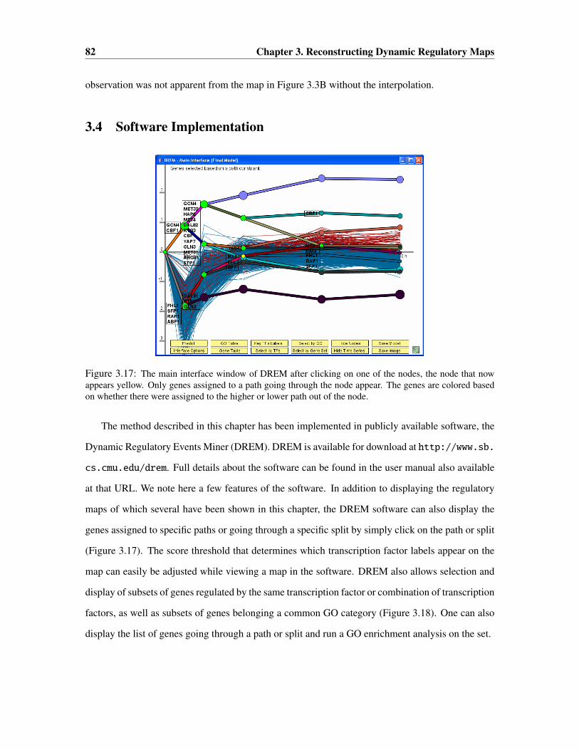
82 Chapter 3. Reconstructing Dynamic Regulatory Maps
observation was not apparent from the map in Figure 3.3B without the interpolation.
3.4 Software Implementation
Figure 3.17: The main interface window of DREM after clicking on one of the nodes, the node that nowappears yellow. Only genes assigned to a path going through the node appear. The genes are colored basedon whether there were assigned to the higher or lower path out of the node.
The method described in this chapter has been implemented in publicly available software, the
Dynamic Regulatory Events Miner (DREM). DREM is available for download at http://www.sb.
cs.cmu.edu/drem. Full details about the software can be found in the user manual also available
at that URL. We note here a few features of the software. In addition to displaying the regulatory
maps of which several have been shown in this chapter, the DREM software can also display the
genes assigned to specific paths or going through a specific split by simply click on the path or split
(Figure 3.17). The score threshold that determines which transcription factor labels appear on the
map can easily be adjusted while viewing a map in the software. DREM also allows selection and
display of subsets of genes regulated by the same transcription factor or combination of transcription
factors, as well as subsets of genes belonging a common GO category (Figure 3.18). One can also
display the list of genes going through a path or split and run a GO enrichment analysis on the set.

3.5. Discussion 83
Figure 3.18: Screenshot of windows in DREM to (left) select a subset of genes belonging to a GOcategory or (right) regulated according to the input by a specific transcription factor or combinationof them.
3.5 Discussion
The availability of gene expression data along with transcription factor-gene association data, such
as ChIP-chip and motif data, has led to a number of efforts aimed at reconstructing regulatory
networks. To date, these efforts primarily focused on determining a static graph representation of
the underlying network. These efforts have led to many insights regarding the overall organization
of networks [10], network motifs [115], and the set of interactions in various biological systems [9,
69, 135, 163, 192].
The computational method we presented in this chapter, DREM, takes a different approach pro-
viding a global dynamic view of the gene regulation. This approach has a number of advantages
when compared to methods that derive static graphs. First, biological systems are dynamic. Tran-
scription factors may bind different genes at different time points. Thus, the ability of DREM to
derive dynamic maps that associate transcription factors with the genes they regulate and their ac-
tivation time points may lead to better insights regarding the system being studied. These insights
may include the identification of master regulators that control the initial response and secondary
regulators that are responsible for more specific pathways. It may also help explain several aspects

84 Chapter 3. Reconstructing Dynamic Regulatory Maps
of the observed response including the condition-specific activity of factors and the activation of
certain network motifs. As timing is available in these maps, some of the paths and the factors regu-
lating them may be linked to predictions regarding the timing of specific phenotypes. Second, many
transcription factors are post-transcriptionally regulated. For these transcription factors, it is hard
to determine an activation time when using only their expression data. When studying biological
systems using ChIP methods, researchers rely on previous knowledge and other data sources to de-
termine which factors to profile under the condition of interest [9, 60, 59, 192]. DREM’s ability to
use general motif data or ChIP based data from other experimental conditions for deriving temporal
regulatory maps presents a useful complementary approach for selecting which transcription factors
to study with a ChIP based experiment. As we have shown for Ino4, these predictions may lead to
new regulatory roles for some of the factors. Importantly, for these factors, DREM also indicates a
time point at which these ChIP-chip experiment should be carried out. Determining the right point
leads to a more accurate set of regulators as we have shown with Gcn4 in MMS. Finally, we note
that although we presented DREM in the context of analyzing several stress-response data sets, it
can be applied equally well to study a single condition of interest.
The accuracy of the models generated by DREM and their predictive power is another indicator
to the importance of data integration. As was noted in the past [72], each data source provides only
a partial view of the activity in the cell. By integrating diverse data sets, we can improve over the
results obtained by each datum on its own. For example, in the context of clustering expression
data, a key question is the number of clusters to use. Another problem relates to noise and the small
number of time points measured. DREM addresses these problems by integrating transcription
factor-gene association data with the time series data. This leads to more natural derivations of
clusters based on bifurcation points and improves the resulting clusters as we showed using GO
(Figure 3.14).
Like any other computational method, DREM is highly dependent on the input data. DREM
relies on the availability of high-quality time series expression data. Here, the sampling rate may
play an important role in the ability of DREM to derive accurate regulatory maps. For example, al-

3.5. Discussion 85
though we observed initial activation by a few master regulators in a number of different conditions,
the initial response to peroxide was determined to be controlled by nine transcription factors. This
may be the result of the sampling rate. If this rate is too low, regulatory effects may be aggregated in
some of the time points, preventing DREM from associating transcription factors with their correct
activation time. Determining the appropriate sampling rate is an important problem [170]. In some
cases, DREM can be used to identify a problem with the sampling rate that has been used and to
suggest places in which more samples are needed. However, even in cases in which an experiment
is well sampled, transcription factor labels can aggregate at earlier time points, as assignments of
genes to paths is based on all time points.
The models derived by DREM are currently limited to tree structures with the option to also
model convergence of paths from a common split. Although this is motivated by previous biological
observations [7], in some cases it may be more natural to allow other types of path merges and
re-splits. DREM also does not explicitly model regulation through other mechanisms, such as
chromosome remodeling and mRNA degradation. Transition probabilities in DREM are computed
using logistic regression, which does not capture all types of combinatorial interactions. Another
limitation of DREM is that the output dynamic map model is sometimes chosen from a number
of possible dynamic maps with similar scores. However, when this happens, these different maps
usually share most of the important splits.
In this chapter DREM was applied exclusively to learn networks in yeast where there is exten-
sive ChIP-chip data available to form the transcription factor-gene association input. In the next
two chapters we discuss computational approaches that can be used for some organisms to predict
transcription factor-gene association data when genome wide ChIP based data is not available for
the transcription factors. Computational methods to predict transcription factor-gene interactions as
well as the growing availability of direct data from high-throughput ChIP based experiments will
make it possible to use DREM with time series expression data from many different species such as
E. coli, human, mouse, and flies, among others. The ability to derive dynamic networks from such
data may lead to new insights, predictions, and ultimately better understanding of many biological

86 Chapter 3. Reconstructing Dynamic Regulatory Maps
systems.

Chapter 4
A Semi-Supervised Method forPredicting Transcription Factor-GeneInteractions in Escherichia coli∗
4.1 Introduction
In the previous chapter we demonstrated the use of DREM in modeling gene regulation dynamics
in the model organism S. cerevisiae. In this chapter we consider another important model organism,
the bacterium E. coli. A challenge in applying a method that requires transcription factor-gene
interactions as input, such as DREM, to E. coli is that, unlike in S. cerevisiae, there is only a handful
of data sets for which experimentally determined genome wide transcription factor binding location
is available [53, 54, 55, 56, 125, 186]. In this chapter we address this challenge by developing a
computational method to predict transcription factor-gene interactions in E. coli.
Decades of research on E. coli have led to the accumulation of a large knowledge base about
transcriptional regulation. Researchers have electronically encoded in databases (such as EcoCyc
and RegulonDB) thousands of activation and repression relationships among transcription factors
∗The content of this chapter is based on the paper [39].
87

88Chapter 4. A Semi-Supervised Method for Predicting Transcription Factor-Gene
Interactions in Escherichia coli
and genes [79, 152, 153]. However, while E. coli has one of the most comprehensive datasets of
experimentally verified transcriptional regulatory interactions of any organism, it is still far from
complete. For instance, the experimentally verified and curated transcription factor-gene interac-
tions provides regulatory relationships for only approximately 1000 genes, which is well below
the more than 4000 genes predicted to be present in E. coli. This relatively low coverage of the
experimentally verified and curated interaction network presents a challenge when attempting to
reconstruct the active regulatory network for a condition of interest based on microarray gene ex-
pression data. When analyzing microarray experiments, researchers often need information about
the set of genes predicted or known to be regulated by various transcription factors. This information
can then be used to determine the influence of the transcription factors in the condition of interest
by indirectly observing the activity of the regulated genes, even for cases in which the transcription
factor is post-transcriptionally regulated [41, 45, 75].
A traditional computational approach to identify additional gene targets of a transcription factor,
which has been applied to E. coli, is to characterize the DNA sequence binding preferences of a
transcription factor based on an alignment of known binding sites of the transcription factor, and
then use this alignment to scan the promoter region of genes for sites matching the preferences [147]
(see also Chapter 1). In some cases researchers have used conservation as an additional filter [57,
76, 182] or extended the alignment based approach using a biophysical based model [148]. While
it has been shown that for some transcription factors in E. coli the presence of a motif can be highly
predictive of true binding [186], for other transcription factors the motif pattern is more degenerate
leading to reduced accuracy. An additional limitation in E. coli, where genes are organized into
transcriptional units and many transcription factors function as both activators and repressors [152],
is that motif scanning only determines the binding site location, which is not sufficient to determine
if a specific binding site is being used to activate or repress a specific gene [4].
Another approach researchers have taken to predicting transcription factor-gene interactions
utilizes just mRNA expression data by evaluating whether the expression level of the transcription
factor and the target gene are consistent with a regulatory relationship. Faith et al. [42] surveyed and
4.1. Introduction 89
evaluated a number of these methods using a compendium of E. coli gene expression data. They
also introduced a new method for this task: The context likelihood of relatedness (CLR) which
extends Relevance Networks [22]. CLR was found to be the top performing method by Faith et al.
at recovering known interactions. Other methods considered by Faith et al. include ARACNe [105],
Bayesian Networks [43] and linear regression networks. The Relevance Network approach directly
ranks transcription factor-gene interactions based on a statistical measure such as the correlation
coefficient or mutual information of the expression profile pairs. CLR extends Relevance Networks
by considering the distribution of values obtained by the statistical measure for all pairs involving
the same transcription factor or regulated gene. The authors found in their evaluation that for CLR
and Relevance Networks the best results were obtained using mutual information and the square of
the correlation coefficient, respectively. As these methods predict network interactions exclusively
from expression data this provides the advantage of being broadly applicable to organisms for which
prior knowledge on gene regulation is limited. However in the case of E. coli, these methods are
unable to take advantage of known interactions or DNA sequence binding information to improve
the accuracy of the predicted interactions. In particular these methods can only identify interactions
for factors that are transcriptionally regulated, which may lead to missing many interactions for
post-transcriptionally regulated factors.
In this chapter we introduce a new method, SEREND (SEmi-supervised REgulatory Network
Discoverer), to predict transcription factor-gene regulatory interactions in E. coli (Figure 4.1).
SEREND is an iterative semi-supervised computational prediction method that takes advantage of
known regulatory interactions in E. coli and extends them by leveraging transcription factor se-
quence binding affinities and a compendium of expression data. Similar to other methods [41, 45,
75], SEREND does not assume that a transcription factor is necessarily transcriptionally regulated.
Instead SEREND uses expression data in the context of known or predicted transcription factor-
gene interactions. However, these previous methods assume a fixed set of transcription factor-gene
interactions, while the purpose of SEREND is to predict additional transcription factor-gene inter-
actions. These predictions can later be used as input to these other methods, as we demonstrate for

90Chapter 4. A Semi-Supervised Method for Predicting Transcription Factor-Gene
Interactions in Escherichia coli
one method on a new expression dataset. Other methods performed iterative analysis as SEREND
does here [16, 69]. However, unlike SEREND, which focuses on classification, the goal of these
prior methods was clustering or gene set module identification leading to different treatment for the
features used and different meanings for the resulting sets. Another method [175] used curated in-
teractions and expression data along with Gene Ontology (GO) and phylogenic similarity to predict
additional gene targets, but did not use an iterative or semi-supervised approach or motif informa-
tion as we do here. We chose for our method not to use GO annotations in generating predictions
giving us the advantage of being able to use GO for an unbiased assessment of the functional role
of predicted targets.
4.2 SEREND Method: Ranking Target Predictions for a Transcrip-
tion Factor
Figure 4.1 outlines our strategy to generate ranked predictions of additional targets of a transcription
factor, including the direction of the interaction (activator or as a repressor). We first extracted from
EcoCyc 11.5 all genomic targets of transcription factors among the 4205 genes that we considered
that have been validated by direct experimental evidence. Only those interactions with the evidence
annotations of ‘Site Mutations’, ‘Binding of Cellular Extracts’, or ‘Binding of Purified Proteins’
were accepted as direct evidence. We also extracted the directions of these interactions. This gave
us 1760 interactions corresponding to 123 transcription factors and 974 genes. See Table S1 of [39]
for the distribution of the number of confirmed targets across transcription factors.
We also obtained the expression value of all the genes across a diverse set of 445 experimental
conditions based on a previously assembled compendium including genetic knockout experiments,
overexpression experiments, and environmental stress conditions [42]. We used the Robust Multi-
chip Average (RMA) normalization, which was reported to represent the optimal way of normaliz-
ing this microarray data from divergent sources among the several major methods considered [42].
We then transformed the data such that each expression value for a gene was the log base two ratio

4.2. SEREND Method: Ranking Target Predictions for a Transcription Factor 91
Figure 4.1: Method overview. SEREND takes as input a compendium of expression data [42], a curated setof E. coli transcription factor-gene interactions with direct evidence [79], and scores for transcription factor-gene motif association based on the PWMs present in RegulonDB [152]. SEREND uses a logistic regressionensemble-based classification method where all non-confirmed targets were initially treated as unregulated bythe transcription factor. SEREND then relaxed this assumption using a self-training method. We evaluated theranked predictions of SEREND using published ChIP-chip data, and by combining SEREND’s predictionswith a new set of time series gene expression data on aerobic-anaerobic shift response in E. coli.

92Chapter 4. A Semi-Supervised Method for Predicting Transcription Factor-Gene
Interactions in Escherichia coli
of its expression value with its average expression value over all the experiments. We excluded from
the compendium 140 previously purported genes from this dataset that were no longer considered
to be among the 4205 true genes in EcoCyc version 11.5.
Finally for 71 of the 123 transcription factors we obtained a Positional Weight Matrix (PWM)
from RegulonDB. We used these matrices to determine a score for the maximum agreement of the
transcription factor with a potential binding site at the promoter region of each gene. For the motif
scanning we used the E. coli K12 genome version U00096.2 sequence. The score of a site is the log-
ratio of the probability of observing the sequence under a PWM model compared to a background
model, which is similar to the approach of [147]. We used a zero order background model, so under
both the PWM and background model, the probability of a site is the product of the probability at
each position. Under the background model we set the probability of observing a specific nucleotide
to its overall proportion in non-coding regions. Under the PWM model, we set the probability of
observing a specific nucleotide at a specific position to the ratio of the count for the nucleotide
at that position over the total counts at the position in the PWM (see Chapter 1). We added a
pseduo-count to each entry in the matrix equal to the non-coding region background probability
of the corresponding nucleotide. For each gene we obtained its RegulonDB transcriptional unit
assignment, which is based on either experimental evidence or computational inference. Six genes
were not annotated as belonging to any transcriptional unit, and for these we assumed each was the
only gene in their respective transcriptional units. We then determined the first gene transcribed in
the gene’s transcriptional unit, and the location of the start of the coding sequence of the gene from
RegulonDB. We then scanned 50 base pairs downstream of the start of the coding sequence and
300 base pairs upstream, on both strands, recording the highest scoring motif hit. If the gene was
annotated to belong to multiple transcription units with different first genes we took the value of the
highest scoring site in any of the regions. If the highest score site for a gene was below 0 we set
the gene’s motif score to 0. In the Supporting Results of [39] there is a plot of the distribution of
the number of maximum scoring sites at each position relative to the start of the coding sequence
of the first gene. From this plot we observed a leveling off of the number of maximum scoring sites

4.2. SEREND Method: Ranking Target Predictions for a Transcription Factor 93
by 50 base pairs downstream and 300 base pairs upstream. For the 52 transcription factors without
a PWM, the motif score was set to a constant 0, but otherwise the method remains the same.
We next used this data to obtain a ranked prediction of new interactions for each transcription
factor. Our method, SEREND, would first train two logistic regression classifiers for each tran-
scription factor. The first classifier is a three-way classifier that uses the expression compendium to
predict whether a gene is activated by, is repressed by, or is not a target of the transcription factor.
A challenge in training such a classifier is that there is no available list of genes which are con-
firmed not to be targets of the transcription factor (negative information). SEREND initially sets
the label for all genes without confirmed evidence in EcoCyc to not being regulated by the tran-
scription factor, though later the method will revisit these assignments. The second classifier uses
motif information, specifically the score of the best binding site of the transcription factor for each
gene. The motif classifier labels are binary, denoting whether a gene is a target of the transcription
factor or not. Initially these labels also correspond to whether or not there is direct evidence in Eco-
Cyc supporting the interaction. The output of these two classifiers are then combined using a third
“meta” logistic regression classifier. The reason we had SEREND keep the two sets of features sep-
arate initially is because of the large number of expression features, as opposed to the single motif
feature. A classifier that directly uses both motif and expression data would likely be vastly empha-
sizing the expression data, whereas by combining the two classifiers SEREND can learn accurate
weights independent of the available features. This approach is similar to ensemble methods such
as stacking [191] and mixture of experts [70].
As we noted above, to generate a negative set SEREND used all genes without a direct evidence
annotation in EcoCyc. While a vast majority of the genes in this set are indeed not regulated by
the transcription factor, some are real targets that have not been discovered to date. We thus had
SEREND modify the labels for some of these genes using a type of semi-supervised classification
method called self-training [203]. Semi-supervised methods of classification use unlabeled data in
conjunction with labeled data to improve classification (Figure 4.2). The self-training method of
SEREND would change the label of genes from not being regulated by a transcription factor to

94Chapter 4. A Semi-Supervised Method for Predicting Transcription Factor-Gene
Interactions in Escherichia coli
being regulated by the transcription factor if the probability with which the meta-classifier classifies
the gene for being regulated by the transcription factor was sufficiently higher than expected. The
method then combined these new target predictions with the targets from the previous iteration and
used them in a new iteration to re-train a classifier and repeated the process until convergence (no
labels changed during an iteration).
Figure 4.2: Motivating the self-training method. We abstractly represent the space of expression featurevalues in two dimensions (though in reality they form a high-dimensional space). The symbol (‘+’) repre-sents an activated target of the transcription factor and the symbol (‘?’) represents genes for which we haveno information for this transcription factor. In this example, the ?’s on the left side of the rectangles areactually true targets of the transcription factor, while those on the right are not. Without self-training weassume all unknown genes are unregulated by the transcription factor (denoted by ‘0’) when forming ourfinal classification boundaries. On the right, the self-training procedure would change the labels of some ofthe unknown genes to being activated targets of the transcription factor before the final classification, whichleads to a better classification boundary.

4.2. SEREND Method: Ranking Target Predictions for a Transcription Factor 95
We will now describe in more formal terms the SEREND method. We will first define SEREND’s
use of logistic regression in general terms and then discuss the specifics of the three classifiers.
When discussing terms specific to a classifier we use a superscript E for the expression classifier, S
for the sequence motif classifier, and C for the meta-classifier.
Logistic regression. Let N be the number of genes (for this application N = 4205), and p be the
number of features to the classifier. Let xi = (xi1, ..., xip) where xi j denotes the value of feature j for
gene i, where i ranges from 1 to N. Let M be the number of classes, and let wim denote the weight
with which gene i is of class m, where m ranges from 1 to M. Usually wim is a binary variable
taking the value 0 or 1, but there is one exception for our application described below. Let Yim be
an indicator variable that gene i is of class m. We define
P(Yim = 1|xi) =eβm0+
∑pj=1 βm j xi j
1 +∑M
c=2 eβc0+∑p
j=1 βc j xi j(4.1)
and we set βm j = 0 for all j when m = 1. The variables βc j are determined by maximizing the
following function:
N∑i=1
M∑m=1
(wim)ln (P(Yim|xi))
− λ M∑
m=2
p∑j=1
β2m j (4.2)
where λ is the regularization parameter, that we selected based on a limited cross-validation analysis.
The Weka logistic regression implementation [190] was used to maximize the function above.
Expression classifier. For the expression classifier SEREND used 445 features (p = 445), and the
features for a gene were its value in each of the expression experiments from a compendium [42]
after the preprocessing described above. For each transcription factor SEREND considered, the
number of classes, M, was three, corresponding to a gene being activated by the transcription factor
(m = 1), repressed by the transcription factor (m = 2), or not regulated by the transcription factor
(m = 3). Let wEim denote the weight with which gene i was of class m. SEREND initially assumed

96Chapter 4. A Semi-Supervised Method for Predicting Transcription Factor-Gene
Interactions in Escherichia coli
all genes without direct evidence in EcoCyc [79] were not regulated by the transcription factor, that
is wEi3 = 1, wE
i1 = 0, and wEi2 = 0. If the gene was only curated with direct evidence to be activated by
the transcription factor, then wEi1 = 1, wE
i2 = 0, and wEi3 = 0. Likewise if the gene was only curated
with direct evidence in EcoCyc to be repressed by the transcription factor, then wEi2 = 1, wE
i1 = 0,
and wEi3 = 0. If the gene was curated with direct evidence to be a target of the transcription factor,
but not only activated or only repressed by the transcription factor, SEREND set wEi1 = n1/(n1 + n2),
wEi2 = n2/(n1 + n2), and wE
i3 = 0 where n1 and n2 are the number of genes uniquely annotated to
be activated and repressed by the transcription factor respectively (if both n1 and n2 were zero, then
wEi1 and wE
i2 were both initialized to 0.5). λE was set to 10.
Sequence motif classifier. For the motif classifier there was a single feature (p = 1), and this feature
represented the maximum agreement of the transcription factor’s PWM with a potential binding site
in the gene’s promoter region based on our motif scanning. The number of classes, M, was two with
m = 1 corresponding to the class that the gene was regulated by the transcription factor and m = 2
if the gene was not regulated by the transcription factor. SEREND set wSi1 = 1 and wS
i2 = 0 if gene
i was curated with direct evidence in EcoCyc to be regulated by the transcription factor, without
respect to whether the transcription factor functions as an activator or repressor of the gene. If the
gene was not in EcoCyc with direct evidence then SEREND set wSi1 = 0 and wS
i2 = 1. λS was set to
1.
Meta-classifier. The meta-classifier had two features, (p = 2), for a gene i. The first feature was the
sum of the activated and repressed probabilities with which the expression classifier would classify
a gene, that is P(YEi1 = 1|xE
i ) + P(YEi2 = 1|xE
i ). The second feature was the probability the motif
classifier gave to the gene for being regulated by the transcription factor, that is P(YSi1 = 1|xS
i ).
SEREND set wCi1 = 1 and wC
i2 = 0 if gene i was annotated with direct evidence in EcoCyc to be
regulated by the transcription factor, otherwise SEREND set wCi1 = 0 and wC
i2 = 1. Genes that were
not in EcoCyc with direct evidence were ranked by the value P(YCi1 = 1|xC
i ). λC was set to 1.
Self-training procedure. The self-training procedure would change the labels of genes that were
previously annotated not to be regulated by the transcription factor to being regulated by the tran-

4.2. SEREND Method: Ranking Target Predictions for a Transcription Factor 97
scription factor if the meta-classifier described above found sufficient evidence that the gene was
regulated by the transcription factor (see Figure 4.2). The criterion for re-labeling such a gene was
that
P(YCi1 = 1|xC
i ) > k
∑N
j=1 wCj1
N
(4.3)
where k is a parameter >1. To provide justification for this criterion we note that a property of a
logistic regression classifier is that the sum of the probabilities for a class equals the count of the
observed instances for the class [61] that is we have
N∑i=1
P(YCi1 = 1|xC
i ) =
N∑j=1
wCj1 (4.4)
The∑N
j=1 wCj1
N term in the criterion for re-labeling a gene would thus be equal to P(YCi1 = 1|xC
i ) if
the probability of being regulated by the transcription factor was uniform across all genes. If the
criterion for re-labeling a gene was satisfied, then the classifier gave greater probability than uniform
that the gene was regulated by the transcription factor, even though the classifier was trained with
the input that the gene was not regulated by the transcription factor. As k increases, the greater
the probability as compared to uniform would be needed to re-label the gene. For all of the self-
training results in this chapter we set k to 2, except for the analysis of the effect of the setting of this
parameter (Figure 4.3). In that analysis k = 2, was among the best settings of the parameter values
considered. In general once the proportion of labeled regulated genes exceeds 1k , it is no longer
possible for an unlabeled gene to satisfy Equation 4.3. Thus when k is set to 2, we have the property
that if majority of genes are labeled as regulated, then the self-training algorithm will not change
any more unlabeled genes to having the label of being regulated.
If the criterion was met to re-label a gene as being a target of a transcription factor then SEREND
set wCi1 = 1, wC
i2 = 0, wSi1 = 1, wS
i2 = 0, and wEi3 = 0. Also for all genes for which wE
i3 = 0, at the
start of the iteration or after the relabeling, SEREND set wEi1 = 1 and wE
i2 = 0 if P(YEi1 = 1|xE
i ) ≥

98Chapter 4. A Semi-Supervised Method for Predicting Transcription Factor-Gene
Interactions in Escherichia coli
P(YEi2 = 1|xE
i ) otherwise SEREND set wEi2 = 1 and wE
i1 = 0. Note that this step specifies a prediction
of the more likely direction of interaction for dual instances, and can change the direction for a
curated target if inconsistent with other curated targets of the same direction (this occurred for
only a relatively small percentage of genes, see Table S1 of [39]). The method terminates when
no change was made to any wim for any of the classifiers. At no point in this procedure was a
gene label changed from being regulated by the transcription factor to not being regulated by the
transcription factor. Again the genes that are not in EcoCyc with direct evidence were ranked by the
value P(YCi1 = 1|xC
i ).
Combining Predictions Across Transcription Factors. The above method gives a ranking of
most likely targets of a transcription factor. For some applications it is useful to have a fixed set of
predictions. For such applications in this chapter, we chose to double the size of the curated network
by simply taking for each transcription factor the same number predictions as there were confirmed
targets of the transcription factor in the input.
4.3 Results
In Table 4.1, we present SEREND’s top prediction for the 25 transcription factors with the most
curated targets in our input set. We note that six of these predictions are already curated in EcoCyc
based on indirect experimental evidence (this information was not used when training). We also
provide in Table 4.1 brief comments on many of these interactions based on a literature search. In
a number of cases we found additional evidence to support the predictions, including in some cases
direct evidence that is not presently curated into EcoCyc.
In evaluating SEREND, we establish in Section 4.3.1 that SEREND can successfully recover
many direct gene targets implicated in Chromatin Immunoprecipitation on chip (ChIP-chip) exper-
iments and compare its ability to do so with other methods. In Section 4.3.2 we then discuss the
biological function of newly predicted targets of some of the major global regulators using a GO
analysis. To further test the predictive capability of SEREND and to assess the functional relevance
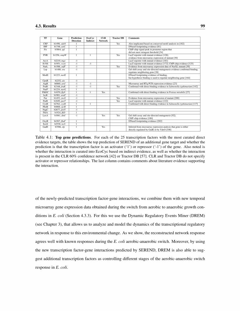
4.3. Results 99
TF Gene Prediction EcoCyc CLR Tractor DB CommentsDirection Indirect Network
CRP b1498, ydeN 1 Yes Also implicated based on conserved motif analysis in [182]IHF b1748, astC 1 DNaseI footprinting evidence [81]Fis b3864, spf 1 ChIP-chip signal peak in promoter region that
did not meet stringent threshold [54]FNR b1256, ompW 1 1 Yes LacZ reporter with mutant evidence [128];
evidence from microarray expression of mutant [30]ArcA b2210, mqo -1 LacZ reporter with mutant evidence [181]H-NS b1951, rcsA -1 -1 LacZ reporter with mutant evidence [172]; ChIP-chip evidence [125]NarL b1588, ynfF -1 Yes Evidence from microarray expression data of NarXL mutant [30]Lrp b1480, sra -1 Gel shift assay and site-directed mutagenesis evidence confirmed binding,
regulates neighboring gene [20]ModE b1223, narK 1 DNaseI footprinting evidence of binding,
but hypothesis binding is used to regulate neighboring gene [164]CpxR b2252, ais -1ArgR b0860, artJ -1 -1 Microarray and RTq-PCR expression evidence [23]FruR b2168, fruK -1 -1 Yes Confirmed with direct binding evidence in Salmonella typhimurium [142]NarP b1224, narG 1
FlhDC b1070, flgN 1 1 Yes Confirmed with direct binding evidence in Proteus mirabilis [27]IscR b1901, araF -1Fur b1452, yncE -1 Yes Evidence from microarray expression of mutant [200]
PurR b1849, purT -1 Yes LacZ reporter with mutant evidence [122]CysB b2762, cysH 1 1 Confirmed with direct binding evidence in Salmonella typhimurium [117]PhoB b4068, yjcH 1NagC b2677, proV -1FhlA b1924, fliD 1LexA b1061, dinI -1 Yes Yes Gel shift assay and site-directed mutagenesis [92];
ChIP-chip evidence [186]OxyR b4367, fhuF 1 DNaseI footprinting evidence [202]SoxS b2530, iscS 1GadE b3506, slp 1 Yes Inferred from microarray expression analysis that gene is either
directly regulated by GadE or by YdeO [108]
Table 4.1: Top gene predictions. For each of the 25 transcription factors with the most curated directevidence targets, the table shows the top prediction of SEREND of an additional gene target and whether theprediction is that the transcription factor is an activator (‘1’) or repressor (‘-1’) of the gene. Also noted iswhether the interaction is curated into EcoCyc based on indirect evidence, as well as whether the interactionis present in the CLR 60% confidence network [42] or Tractor DB [57]. CLR and Tractor DB do not specifyactivator or repressor relationships. The last column contains comments about literature evidence supportingthe interaction.
of the newly-predicted transcription factor-gene interactions, we combine them with new temporal
microarray gene expression data obtained during the switch from aerobic to anaerobic growth con-
ditions in E. coli (Section 4.3.3). For this we use the Dynamic Regulatory Events Miner (DREM)
(see Chapter 3), that allows us to analyze and model the dynamics of the transcriptional regulatory
network in response to this environmental change. As we show, the reconstructed network response
agrees well with known responses during the E. coli aerobic-anaerobic switch. Moreover, by using
the new transcription factor-gene interactions predicted by SEREND, DREM is also able to sug-
gest additional transcription factors as controlling different stages of the aerobic-anaerobic switch
response in E. coli.

100Chapter 4. A Semi-Supervised Method for Predicting Transcription Factor-Gene
Interactions in Escherichia coli
4.3.1 Evaluation of Predictions: Comparison with ChIP-chip Data
We first evaluate here the ability of SEREND under different settings of the self-training parameter,
k, to predict gene targets implicated in ChIP-chip experiments for five global regulators: CRP [55],
Fis [54], FNR [53], IHF [54], and H-NS [125]. We then for one of these parameter settings com-
pared with several other methods. For each of the ChIP-chip experiments we extracted the interac-
tions that are not currently present in the EcoCyc database with direct evidence for the 4205 genes
that we considered. As the authors of these papers only reported the genes immediately adjacent to
or overlapping the signal peak, we extended their lists to include any gene sharing the same tran-
scriptional unit based on the RegulonDB defined transcriptional units. The total number of gene
targets in these sets for CRP was 148, for Fis was 347, for IHF was 199, for FNR was 131, and
for H-NS was 1191. For H-NS, there is another list of ChIP-chip based targets [54] separate from
those of [125]. We note that these sets of genes will not necessarily include all genes regulated
by the transcription factor. In some cases these transcription factors have been reported to bind at
many places in the genome with a weaker and more ambiguous signal level than for the lists we
are using [54, 55]. In other cases targets of a transcription factor may not be recovered because
of condition specific binding or technical limitations of the ChIP-chip protocol [53]. Despite these
limitations, we still consider these lists to be a valuable resource for comparing methods aimed at
identifying additional direct targets of a transcription factor.
Analysis of the Effect of the Value of the Self-Training Parameter
As mentioned above the self-training parameter determines the threshold for changing a previously
unlabeled gene to being regulated. As k increases the self-training method requires greater confi-
dence from the classifier that the gene is actually regulated by the transcription factor before chang-
ing its label. When k is sufficiently high, no gene will be relabeled as a target of the transcription
factor making the SEREND method similar to a version that does not use self-training. The results
will not necessarily be identical for such k since the results without self-training did not modify ac-
tivator versus repressor labels, while the version with self-training is able to change labels between

4.3. Results 101
Figure 4.3: The effect of the value of the self-training parameter, k, on predicting ChIP-chip implicatedgene targets. The graphs show an evaluation of SEREND for setting k to 1.5, 2, 4, and 10 in terms ofpredicting targets of the global regulators CRP [55], Fis [54], FNR [53], H-NS [125], and IHF [54] implicatedby ChIP-chip experiments, but not curated into the EcoCyc database with direct evidence. We also showresults here for a version of SEREND without the self-training step. The x-axis represents the number ofpredictions made by the method (excluding targets already in EcoCyc with direct evidence), and the y-axisrepresents the cumulative number of matches recovered. Note the x-axis scale for CRP and the y-axis scalefor Fis and H-NS are different than the others.

102Chapter 4. A Semi-Supervised Method for Predicting Transcription Factor-Gene
Interactions in Escherichia coli
activator and repressor even if not changing any unlabeled genes to being regulated.
In Figure 4.3 we evaluate the SEREND predictions when k is 1.5, 2, 4, and 10. We also com-
pare in this figure to a version of SEREND that does not use self-training. In Figure 4.3, we plot
separately for each transcription factor on the x-axis the number of gene predictions a method made
up to either 500, or in the case of CRP 700, excluding predictions that already have direct evidence
in EcoCyc. On the y-axis, we show the number of matches to the set of genes in our ChIP-chip
defined gene set, for each number of predictions. For k = 1.5 and k = 2, we observe a substantial
improvement from the self-training procedure in the FIS, IHF, and H-NS cases, though there is a
performance drop in the FIS case as compared to k = 2. For k = 4, we again see substantial im-
provement in the FIS and H-NS cases from self-training, while in the IHF case the improvement
gained from the self-training is only marginal. For k = 10, we no longer observe an improvement
from self-training in the case of FIS and IHF, and only a small improvement for H-NS indicating
the self-training method in these cases is becoming too restrictive as to which genes it will relabel.
In the FNR case, we did observe a small improvement from the self-training when k = 4 and k = 10
that we did not observe for k = 1.5 or k = 2. In our evaluation, we did not observe an overall
benefit from self-training in the CRP case for any parameter value of k that we considered. All the
subsequent results will be based on the parameter choice k = 2.
Comparison with other Methods
In addition to comparing the predictions of SEREND (with k = 2) to those that would be gen-
erated by it if it did not use the self-training procedure, we also compare here these results to
motif-based predictions and the previously reported predictions of the CLR method with mutual in-
formation [42]. In the case of the dimer IHF, CLR gives two different scores corresponding to each
of the subunits, we mapped this to one score by taking the more significant of the two scores. As
a baseline, we also compare the expected number of matches with a method that simply randomly
orders the genes. In each graph, we plot a point representing the number of genes curated in EcoCyc
to be a target of the transcription factor based only on indirect evidence (e.g. gene expression data

4.3. Results 103
Figure 4.4: Comparison of methods to predict gene targets implicated in ChIP-chip experiments. Werepeat the evaluation in Figure 4.3, this time comparing SEREND (with k = 2), the version of SERENDwithout self-training, the CLR method [42], just using our motif values (Motif), and random predictions. Wealso compare at a single prediction level with the genes curated into EcoCyc from the literature as targetsof the transcription factor based on indirect evidence. For CRP and FNR we compare with the Tractor DBpredictions [57] and predictions based on RegTransBase [76], and for H-NS with the results of a differentChIP-chip experiment [54]. The x-axis represents the number of predictions made by the method (excludingtargets already in EcoCyc with direct evidence), and the y-axis represents the cumulative number of matchesrecovered. Note the x-axis scale for CRP and the y-axis scale for Fis and H-NS are different than the others.

104Chapter 4. A Semi-Supervised Method for Predicting Transcription Factor-Gene
Interactions in Escherichia coli
or presence of a binding site motif). For the FNR and CRP graphs we also compare to the Tractor
DB method [57] and a prediction ordering we derived based on RegTransBase, both methods use
motif and conservation information. We generated ranked predictions for a transcription factor in
RegTransBase [76] based on the set of predicted genes returned in the TransTableView for E. coli
K12 using the default setting for sensitivity on the site score, and specifying to measure conserva-
tion based on all genomes for the species E. coli. We ranked all genes returned by RegTransBase,
meaning the gene had one or more binding sites within 400 base pairs upstream or 50 base pairs
down stream of the start of the gene satisfying the sensitivity threshold, based on the maximum
conservation score for a site returned for the gene. We then extended the ranked list to include all
genes in the same transcriptional unit as listed in RegulonDB. When extended for transcriptional
unit a gene received the same site and conservation score, as the highest ranking gene from its tran-
scriptional unit from the original ranked list. Tractor DB did not make any predictions for H-NS,
IHF, and only one for Fis, and RegTransBase did not directly support these transcription factors.
As the charts in Figure 4.4 show, and as we noted above, for Fis, IHF, and H-NS there is a
sizeable improvement for SEREND derived from its use of the self-training procedure. For FNR the
results of SEREND as compared to a version without the self-training procedure are about the same,
and for CRP the version without self-training achieves more matches over the first several hundred
predictions. For all transcription factors predictions from SEREND are better than expected from
randomly ordering genes. We found the motif scores to be significantly predictive of in-vivo binding
for all but one of the transcription factors we looked at. Unlike the other transcription factors, for
Fis higher motif scores were not associated with higher likelihood of binding. Combining the motif
scores with expression data using SEREND led to a clear overall improvement in all cases except for
CRP, where the relative performances varies depending on the number of predictions. Predictions
based on RegTransBase [76] and the Tractor DB [57] method for identifying motif targets, both of
which used conservation information about motifs, did not show overall improvement in recovering
genes in the validation sets for FNR and CRP than just using our motif scores for genes, which does
not consider motif conservation. Interestingly we note our predictions for H-NS are competitive

4.3. Results 105
with the set of targets reported by a second ChIP-chip experiment of [54], indicating that for this
transcription factor the quality of our predictions are within the tolerance expected from differences
in laboratory experimental protocols and other experimental noise. We chose here to use the list
of [125] as the validation set, as it is larger and includes the majority of targets with curated direct
evidence, while at the cutoff at which the list of [54] was derived it includes only one curated direct
evidence target. The plots also indicate that in all cases except for CRP, SEREND either outperforms
or is essentially equivalent to the literature curated interactions without direct evidence, and has the
added benefit of allowing more flexibility in the number of predictions selected.
4.3.2 Biological Functional Analysis of Predicted Targets of Global Regulators
We used a GO enrichment analysis to characterize the biological functions of newly predicted tar-
gets of global regulators and then compared that with an analysis on the set of curated and verified
targets. We performed the analysis based on the European Bioinformatics Institute (EBI) E. coli K12
UniProt GO annotations [24] for each of the seven transcription factors with the most targets in Eco-
Cyc (ArcA, CRP, FIS, FNR, H-NS, IHF, and NarL). In Table 4.2 we list for each transcription factor
the top ranked GO category among its predicted targets along with the enrichment p-value, as well
as the p-value for this category among the curated targets. The reported p-values are uncorrected
p-values computed using the hypergeometric distribution; corrected p-values for multiple hypothe-
sis testing can be found in the Supplementary Results of [39]. We observe that for ArcA, CRP, and
FNR the top ranked GO category based on the predicted targets is significant in the analysis on the
curated targets, which was not the case for FIS, H-NS, IHF, and NarL. For FIS, the most significant
GO category among the new predictions was the structural constituent of ribosome. FIS does have a
known role in regulating ribosomal RNA genes [149], and among our newly predicted targets of FIS
are a significant number of ribosomal proteins. For H-NS, its involvement in transposition has been
previously demonstrated [167]. For IHF, the most significant category was the lipopolysaccharide
biosynthetic and metabolic processes. The role of IHF in capsular polysaccharide biosynthesis has
been previously discussed [189]. For NarL, the parent category of nickel ion binding in the GO

106Chapter 4. A Semi-Supervised Method for Predicting Transcription Factor-Gene
Interactions in Escherichia coli
TF Top GO Category for Predicted Targets p-Value, Predicted Targets p-Value, Curated TargetsArcA Cellular respiration 2 × 10⁻¹⁰ 2 × 10⁻¹⁵
CRP Carbohydrate transport 3 × 10⁻¹⁴ 6 × 10⁻²⁵
Fis Structural constituent of ribosome 2 × 10⁻³³ 0.84FNR 4 iron, 4 sulfur cluster binding 4 × 10⁻³ 3 × 10⁻¹⁴
H-NS Transposition, DNA-mediated 2 × 10⁻⁴ 0.11IHF Lipopolysaccharide biosynthetic/metabolic process 4 × 10⁻¹¹ 1NarL Nickel ion binding 3 × 10⁻⁷ 1
Table 4.2: Top GO categories for predicted gene sets. The table shows the most significant GO categoriesfor new predicted gene targets for the transcription factors (TFs), with the most curated targets in EcoCyc.The table compares the enrichment p-value of this category for the newly predicted targets and the curatedtargets.
hierarchy, transition metal ion binding, was highly significant among curated genes (p-val <10−10).
These results support the assignments made by SEREND and indicate that the newly predicted tar-
gets for most transcription factors can be used to correctly extend our understanding of the function
of these transcription factors.
4.3.3 Application to Aerobic-Anaerobic Shift
The above analysis with ChIP-chip data focused on establishing that SEREND’s predictions are
significantly over-represented within the set of direct binding targets of the transcription factor. We
also evaluated whether the gene expression level of SEREND’s target predictions are consistent
with that of known targets of these transcription factors. Additionally, we tested if the activator and
repressor predictions are accurate for transcription factors that function in both roles. We performed
this evaluation on new temporal microarray gene expression data (Gene Expression Omnibus acces-
sion GSE8323) for the shift from aerobic to anaerobic growth during steady state culture conditions
of E. coli. For details on the experimental procedures used to generate the data see [39]. In this
bacterium, in response to the lack of oxygen in the growth medium, two transcription factors, FNR
(fumarate-nitrate reductase regulator) and ArcA transcription factors (aerobic respiratory control),
are known to be the master regulators of this response. FNR is a key regulator of respiration and
it controls the transcription of many genes whose functions facilitate adaptation to growth under
O2-limiting conditions [74, 128, 129, 154, 155]. Under microaerobic conditions, ArcA induces ex-
pression of several gene products of the central carbon metabolism, which are sensitive to lower
4.3. Results 107
levels of oxygen, and it represses many genes of aerobic respiration [1, 29, 165]. NarL and NarP
are two other transcription factors known to be involved in the aerobic-anaerobic shift response,
and both of them regulate expression of several operons in response to nitrates and nitrites during
anaerobic respiration and fermentation [30, 126, 143]. However, while the roles of the transcription
factors listed above have been well characterized in aerobic-anaerobic response, the identity and
roles of some other transcription factors are less clear.
Comparison of Predicted and Curated Transcription Factor-Gene Interactions Using New
Expression Data
To compare the set of interactions in the curated databases with the new targets predicted by
SEREND, we first focused on expression values measured at the last sampled time point, 55 min
after the shift from aerobic to anaerobic growth. Since these expression values were not used to
generate our predictions they provide an unbiased test set for our predictions. We compared the
average expression of the two sets of targets (curated and new predictions) for each transcription
factor activity mode (i.e., a factor and its influence as an activator or a repressor). In Figure 4.5, we
plot the average expression of the two sets for the top 20 transcription factor activity modes in terms
of the number of new predictions. We also plot a 95% confidence interval based on 10,000 random-
izations for selecting sets of the same size as the new predictions (curated predictions confidence
intervals were similar). Figure 4.5 illustrates a good agreement between the average expression of
the curated targets and the newly predicted targets for this new expression dataset. We observe that
the predicted and curated predictions completely agree on which are the top 8 most significantly
upregulated gene sets and which are the top 5 most significantly downregulated gene sets. From
Figure 4.5 we also observe that on average CRP, FNR, and IHF predicted activated targets had an
induced expression level, while the predicted repressed targets had a repressed expression level.

108Chapter 4. A Semi-Supervised Method for Predicting Transcription Factor-Gene
Interactions in Escherichia coli
Figure 4.5: Transcription factor target set agreement between predicted and curated targets. The aver-age expression values for transcription factor regulatory modes (transcription factor and activator or repressorrelationship) among curated and new predicted targets at the 55-min time point of the new aerobic-anaerobicshift gene expression data are shown. Only the top 20 transcription factor regulatory modes in terms of thenumber of new predictions are included. We excluded genes with dual annotations from the curated averages.We included genes in the predicted set averages for which we had a new prediction with regards to the modeof interaction (either because they were dual-annotated or SEREND predicted the opposite mode; this gener-ally was for a small number of genes; see Table S1 of [39]). For each transcription factor regulatory mode,the graph also displays the 95% confidence interval based on 10,000 random draws of new predicted targetsof the same size set. The graph shows that the average expression for a number of predicted transcriptionfactor target gene sets was significantly induced or repressed. The graph also shows a good agreement formost transcription factor target gene sets between the curated and predicted sets, indicating the accuracy ofthe predictions.
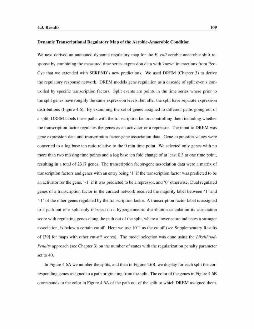
4.3. Results 109
Dynamic Transcriptional Regulatory Map of the Aerobic-Anaerobic Condition
We next derived an annotated dynamic regulatory map for the E. coli aerobic-anaerobic shift re-
sponse by combining the measured time series expression data with known interactions from Eco-
Cyc that we extended with SEREND’s new predictions. We used DREM (Chapter 3) to derive
the regulatory response network. DREM models gene regulation as a cascade of split events con-
trolled by specific transcription factors. Split events are points in the time series where prior to
the split genes have roughly the same expression levels, but after the split have separate expression
distributions (Figure 4.6). By examining the set of genes assigned to different paths going out of
a split, DREM labels these paths with the transcription factors controlling them including whether
the transcription factor regulates the genes as an activator or a repressor. The input to DREM was
gene expression data and transcription factor-gene association data. Gene expression values were
converted to a log base ten ratio relative to the 0 min time point. We selected only genes with no
more than two missing time points and a log base ten fold change of at least 0.3 at one time point,
resulting in a total of 2317 genes. The transcription factor-gene association data were a matrix of
transcription factors and genes with an entry being ‘1’ if the transcription factor was predicted to be
an activator for the gene, ‘-1’ if it was predicted to be a repressor, and ‘0’ otherwise. Dual regulated
genes of a transcription factor in the curated network received the majority label between ‘1’ and
‘-1’ of the other genes regulated by the transcription factor. A transcription factor label is assigned
to a path out of a split only if based on a hypergeometric distribution calculation its association
score with regulating genes along the path out of the split, where a lower score indicates a stronger
association, is below a certain cutoff. Here we use 10−4 as the cutoff (see Supplementary Results
of [39] for maps with other cut-off scores). The model selection was done using the Likelihood-
Penalty approach (see Chapter 3) on the number of states with the regularization penalty parameter
set to 40.
In Figure 4.6A we number the splits, and then in Figure 4.6B, we display for each split the cor-
responding genes assigned to a path originating from the split. The color of the genes in Figure 4.6B
corresponds to the color in Figure 4.6A of the path out of the split to which DREM assigned them.

110Chapter 4. A Semi-Supervised Method for Predicting Transcription Factor-Gene
Interactions in Escherichia coli
Figure 4.6: Inferred dynamic regulatory maps of E. coli response to the aerobic-anaerobic shift. (A)Dynamic regulatory map inferred by DREM by combining the new aerobic-anaerobic shift microarray geneexpression data and our prediction-extended transcription factor-gene interaction dataset. The numberedgreen nodes represent the split points. DREM assigned genes to their most likely path through the splits.Paths out of the splits are annotated with transcription factor regulatory modes that are associated with genesassigned to the path at a score <10−4, and the annotations are ranked ordered using the score. A ‘1’ after thetranscription factor symbol denotes activation mode and a ‘-1’ denotes repression mode. The area of a nodeis proportional to the standard deviation of the expression of the genes traversing through that node. (B) Thegenes traversing through the nine splits are shown in (A). The number in the upper left of the plot correspondsto the number of the split. Genes are colored based on their path out of the split. (C) The DREM map inferredwhen using for the transcription factor-gene input only curated interactions with direct evidence.
4.3. Results 111
The map indicates that by 2 min those genes that were eventually upregulated (gray-colored genes),
already had a different distribution than those which were downregulated (orange-colored genes).
Among GO categories, the upregulated genes were most enriched for carbohydrate transport (p-val
<10−8), while the downregulated genes were most enriched for biosynthetic process genes (p-val
<10−30) including translation genes (p-val <10−24). The map also indicates that between 5 min
and 25 min there was a large change in expression distribution among the genes most activated and
repressed in this condition. The last split event in the map occurs 25 min after the response, and
the paths remain mostly unchanged thereafter, indicating that by 35 min at the transcriptional level
E. coli has adapted to the anaerobic conditions. This also suggests that the transitional events that
have occurred between 0-35 min after switching to an anaerobic state are events associated with
the microaerobic response. The cascade of splits occurring before 25 min of the shift suggests that
E. coli cells are slowly adapting to the anaerobic conditions during the initial phases of the shift.
DREM has also identified several known and new transcription factors as regulators of this shift as
we discuss below.
Comparison to Using Only the Curated Network
The map of Figure 4.6A was based on known targets from EcoCyc and extended with our new
predictions. To determine if the added predictions improved our ability to reconstruct this regulatory
network, we compared this to the map recovered by DREM when using only the curated interactions
from EcoCyc with direct evidence. Figure 4.6C presents the regulatory map identified when using
only the curated interaction data as input. While some of the paths share the same annotations in
both maps, in the vast majority of cases the score is more significant when using the predicted set.
Figure 4.7A presents a scatter plot of the most significant scores of the transcription factors (for
those with scores lower than 0.001). Reassuringly, we observe a substantial increase in significance
for important transcription factors for this response, such as ArcA, FNR, and NarP. As a control,
we considered adding random predictions and found that these did not improve scores but rather
decreased them (see Supplementary Results of [39]).

112Chapter 4. A Semi-Supervised Method for Predicting Transcription Factor-Gene
Interactions in Escherichia coli
Figure 4.7: Impact of using prediction-extended transcription factor-gene input to DREM. (A) x-axis(y-axis) is the maximum of the negative of the log base 10 score of the transcription factor and regulatorymode at any split using the curated transcription factor-gene input (prediction-extended transcription factor-gene input). Any point above the diagonal line received a more significant score using our predictions. Arandomization analysis shows this is not because we used a larger set of interactions input (see SupportingResults of [39]). The negative log base 10 score for Fis (38.2 using our predictions and 5.7 using the curatedEcoCyc list) is not plotted to keep the dimension of the scale reasonable. (B) (Left panel) The expressionof non-filtered genes annotated with direct evidence in EcoCyc as being activated by Fis. Color-coding ofgenes correspond to path assignments between 5 and 10 min in the maps of Figure 4.6. (Center panel) Thegenes in the predictions extended network that are annotated as being activated by Fis. (Right panel) All GO-annotated ribosome genes in the dataset meeting the filtering criteria. There is a significant overlap betweenthese genes and Fis-activated genes in the predicted network.
4.4. Discussion 113
An interesting observation is the large increase in significance of the score of Fis activated genes
when including the predicted interactions. Furthermore, Fis is seen associated with repressed paths
for two splits in Figure 4.6A, but only the first split in Figure 4.6C. In the left panel of Figure 4.7B,
we show the expression of those Fis activated genes that are in the curated input. In the center panel
of Figure 4.7B, we show the expression pattern of those Fis activated targets that are in our predic-
tion extended network. On the right panel in Figure 4.7B, we plot the expression of GO annotated
ribosome genes. When using only the curated data, the mechanism by which these ribosomal genes
are regulated as part of this response is unexplained, as only three of these genes have a regulator
with curated direct evidence. In contrast, when using the new predictions many of these ribosomal
genes are determined to be activated by Fis (31 of the 56 genes, p-val<10−28). Of these 31 genes,
21 are on the list of genes bound by Fis in [54] or are in the same transcriptional unit as a gene from
this list. The potential importance of the effect of Fis in altering the expression of ribosome genes
in response to the aerobic-anaerobic shift is something that would have been missed by the method
had we not extended the curated network with additional predictions.
4.4 Discussion
A large amount of experimental data has accumulated regarding transcription factor-gene regulatory
information for E. coli. However, this information is not complete. Many of the genes in E. coli
do not have any validated regulators and it is likely that many interactions are unknown even for
those genes with one or more validated regulators. To make optimal use of the curated information,
methods should leverage this information as much as possible when making additional predictions
of transcription factor-gene regulatory interactions. Such predictions would then be useful when
combined with other high throughput data measuring responses of all E. coli genes in a condition
of interest.
Here we presented a new semi-supervised learning-based method, SEREND, which uses curated
data, sequence motif information, and a compendium of expression data to predict new transcrip-

114Chapter 4. A Semi-Supervised Method for Predicting Transcription Factor-Gene
Interactions in Escherichia coli
tion factor-gene interactions. Using ChIP-chip data, we have shown that semi-supervised learning
can improve predictions regarding transcription factor-gene interactions. Using new temporal gene
expression data for the aerobic-anaerobic switch response in E. coli, we have shown that these
predictions can improve the utility of experimentally-verified interactions when reconstructing dy-
namic response networks. While the resulting networks utilized some of the new predictions these
are primarily for transcription factors involved in this response. If the transcription factor binds the
DNA without effect on transcription in this condition these interactions would not be identified in
the resulting map.
The resulting regulatory map for the aerobic-anaerobic response summarizes current knowledge
and provides new insights into the role of various transcription factors in the response. The map
labels the activators FNR, CRP, NarP, ModE, FhlA, and H-NS, and the repressors NarL and H-NS
as associated with the upregulated genes, those assigned to the induced path in the first split. This
means that the method predicts these transcription factors to be major regulators of the response,
and likely the first transcription factors to upregulate expression of various genes when oxygen is
removed from the growth medium. As mentioned above FNR, NarL and NarP are well known to be
important regulators in this response. FhlA (formate hydrogen-lyase) is a well known transcriptional
activator of hyc and hyp operons in E. coli, and the FNR-mediated regulation of hyp expression in E.
coli has also been described [114], which might indicate that FhlA acts synergistically with FNR in
regulating some genes during the anaerobic response. Published evidence has suggested that ModE
is a secondary transcription activator of the hyc and the nar operons (encoding genes in response
to nitrates and nitrites) [164] and the dmsABC operon under conditions of anaerobiosis [112]. The
initial repressed pathway includes targets that are associated with activation by Fis, PhoB, and PhoP
(indicating decreased activity of these transcription factors) and repression by FNR and ArcA. Fis
is known to play a major role in reconfiguration of E. coli cellular processes by up-and down-
regulating expression of various genes during changes in growth conditions, and its expression also
varies dramatically during cell growth by autoregulation [127, 120]. Additional transcription factors
that are associated with activated genes at later split events include DcuR, TdcA, TdcR, and IHF.

4.4. Discussion 115
CRP has been described to govern the anaerobic transcriptional activation of the Tdc regulators
(TdcA and TdcR) [157], which supports our findings that these are secondary responders.
While we have used ChIP-chip data in evaluating predictions for some transcription factors,
overall the number of transcription factors for which ChIP-chip data are currently available in E.
coli is limited [53, 54, 55, 56, 125, 186]. In addition, unlike SEREND, ChIP-chip experiments
do not differentiate between activator and repressor relationship. Furthermore SEREND may dis-
cover genes regulated by transcription factors that ChIP-chip experiments would not recover due
to condition-specific binding activity or other experimental noise. Finally there could be cases in
which a transcription factor binding is detected in a ChIP-chip experiment, but a gene regulated by
the transcription factor is not associated with being a target of transcription factor due to the imper-
fect process of mapping a transcription factor binding location to a set of regulated genes. While
motif input is also sensitive to this mapping, the expression input is not, thus in some of these cases
SEREND could still predict the interaction.
One avenue for future work is to extend our semi-supervised methodology to also include data
from ChIP-chip experiments in generating predictions. In S. cerevisiae, a global atlas of transcrip-
tion factor-gene interactions is available based on ChIP-chip data [60], which researchers improved
by combining the ChIP-chip data with other evidence sources, such as sequence motif and gene
co-expression information [17, 60, 64]. Another extension is to apply our methodology for in-
ferring transcription factor-gene interactions in additional model organisms for those transcription
factors with sufficient known target genes. As computational methods for integrating interaction
and expression data become increasingly available, we expect that global atlases of transcription
factor-gene interactions will become increasingly important resources for experimental biologists
to integrate with specific expression experiments.


Chapter 5
Integrating Multiple Evidence Sourcesto Predict Transcription Factor Bindingacross the Human Genome
5.1 Introduction
In this chapter we will present a method to improve the computational inference of locations of
transcription factor binding in the human genome. This then leads to improvements in transcription
factor-gene association predictions, which can be used as input to methods that model gene regula-
tion dynamics such as DREM discussed in Chapter 3. Unlike as we did for E. coli in the previous
chapter we will not assume that we have available a set of high quality experimentally confirmed
gene targets of a transcription factor of interest, which is not available for most transcription factors
in human. We will however assume we have information about the sequence binding preferences
of the transcription factor, that is the motif it recognizes. Between the JASPAR and TRANSFAC
databases [109, 183] there are around 500 positional weight matrices for human curated from the
literature (see Chapter 1). Additionally new high-throughput experimental techniques developed to
determine sequence preferences of transcription factors such as the Protein Binding Microarray Ar-
ray [15] and a bacterial one-hybrid system [121] are leading to the availability of sequence binding
117

118Chapter 5. Integrating Multiple Evidence Sources to Predict Transcription Factor Binding
across the Human Genome
specificities for hundreds of additional transcription factors.
The vast size of the human genome makes detecting regulatory sites a greater challenge than
in organisms with more compact genomes such as E. coli, as there can be many sites which by
chance match well the motif that the transcription factor recognizes, but are not actually bound.
Researchers have attempted to address this issue by filtering sites that did not meet certain restrictive
requirements. For instance in searching for motif hits for a transcription factor, the work of Xie et
al. [194] only considered those sites within 2000 base pairs of a transcription start site and for which
the site was conserved in mouse, rat, and dog. In contrast Sinha et al., [171] did not require evidence
of conservation, but used a more restrictive requirement on the location of motif matches by only
considering regions within 500 base pairs upstream of the transcription start site or 200 base pairs
downstream [171]. Both of these methods would give equal weight to any position within the region
of consideration, but then no weight to a site a single base out of the region. The UCSC Genome
Browser [78] provides predictions of binding sites across the entire genome requiring evidence of
conservation in mouse and rat as does Xie et al. [194], but not requiring conservation evidence in
dog. A method that did not rely on using strict binary rules with regards to general evidence features
about a site, but instead used all information about them to form a probabilistic prior on transcription
factor binding could potentially lead to more accurate identification of truly bound sites.
A prior on transcription factor binding at a specific base in the human genome would convey
a probability estimate that a transcription factor would bind the location, only knowing general
properties of the location (e.g. distance to nearest transcription site and conservation) that are not
specific to any one transcription factor. Previously as there was limited or no full genome data
available on transcription factor binding in human, constructing a prior that effectively integrated
evidence sources would have been extremely challenging. However with the public availability now
of over a dozen data sets with experimental data on the location transcription factor binding across
the human genome [25, 73, 93, 94, 102, 140, 146, 188, 197, 199] we have the opportunity to use a
machine learning approach to construct an empirical prior on transcription factor binding across the
human genome. In addition to these genome-wide data sets on the location of transcription factor

5.2. An Informative Empirical Prior on Transcription Factor Binding 119
binding, high-resolution genome-wide data sets of key genomic properties that can be informative
of transcription factor binding such as DNaseI hypersensitivity [21] and histone modifications [12]
have also become available. With these growing and diverse set of evidence sources, there is an
opportunity for methods to integrate these data sources to improve the prediction of transcription
factor binding.
In Section 5.2 of this chapter we will discuss how we constructed a prior on transcription factor
binding, and then evaluate its effectiveness. In Section 5.3 we discuss and demonstrate how we can
combine the prior with motif information for a transcription factor to improve predictions of regions
bound by a specific transcription factor. Finally in Section 5.4 we will conclude this chapter with a
discussion.
5.2 An Informative Empirical Prior on Transcription Factor Binding
5.2.1 Method to Learn the Empirical Prior
Here we describe how our method learns a function that maps a set of features about a location in
the human genome to an empirical prior probability that a transcription factor binds that location. In
addition to the feature data on any genomic location, the method also uses as training data C data sets
with each data set reporting regions of the genome, of on average about 1000 base pairs in length,
within which a transcription factor is determined to bind based on a full genome experiment. We
note that there are several non-standard aspects of our problem as compared to a standard supervised
machine learning setting. We will discuss these issues, describe our method, and then discuss the
extent to which the method at least partially addresses some of these issues.
In a standard supervised classification setting one assumes that the training and testing data
come from the same underlying distributions. Here we are in a transfer learning setting where we
are primarily interested in applying our prior to predict binding locations for a transcription factor
for which we did not have any training data available. In such cases we cannot expect the testing
data of the bound sites of the new transcription factor to come from the same underlying distribution

120Chapter 5. Integrating Multiple Evidence Sources to Predict Transcription Factor Binding
across the Human Genome
as our available training data, though it will likely be related. A second difference is our labeled
training data is only a small portion of the positively bound sites. This is the case since each training
data set is specific to one transcription factor in one tissue type and condition, while we would like
to learn a prior on transcription factor binding for any transcription factor across any tissue type
or condition. Thus the proportion of the genome bound by a transcription factor in the C training
datasets, will be lower than the proportion of transcription factor binding across the genome that we
would want the prior to infer. Finally, there will be noise and biases in the labeled training data for
several reasons. One reason for this is that the high-throughput experimental data generally does
not tell us exactly where the transcription factor binds, but rather detects that there is binding within
a region of about 1000 bases, with the resolution depending on the technology. A second reason is
the lack of uniformity in what is considered a positively bound region across data sets, both because
of the sensitivity of different technology and variations in using the same technology. A final reason
is that experimental technology is limited in detecting binding within sequences that are not unique
in the human genome.
Our method first learns independently for each of the C data sets a probabilistic classifier (see
below for a discussion of training data sets). To obtain our empirical prior probability of a transcrip-
tion factor binding at a specific base location, the method takes a simple average of the probability
each of the C classifiers gives. For each classifier we used as positive training examples a base
location in the center of each genome region reported to be bound by the transcription factor. As a
negative set we randomly sampled 49 base locations for every one positive location. The randomly
selected locations were restricted to come from the non-gapped regions of the human genome. In
each case we did a stratified random sampling so that for every one real location on a chromosome
we would have 49 randomly selected locations from the same chromosome. Formally the prior
probability the method gave to a single base location in the human genome, b, being bound by a
transcription factor is
P(b| fb) =1C×
C∑c=1
Pc(b| fb)

5.2. An Informative Empirical Prior on Transcription Factor Binding 121
where fb is a vector of feature values specific to genome location b (see below for a discussion of the
set of features used). Pc(b| fb) is the probability a logistic regression classifier gives that a location
with a set of features fb is bound by a transcription factor. Using a logistic regression classifier
gives the advantage of having a well-defined probabilistic output. We used the logistic regression
implementation LR-TRIRLS [83] which could effectively scale to some of our larger training sets
containing over a million data points. We used the default settings of the software which sets the
ridge parameter to 10 (see Chapter 4 for a discussion of logistic regression classification with ridge
loss). If a base is in a gap portion of the genome sequence we automatically set its prior to 0.
Under the method for a base to receive relatively high prior probability it will need to receive a
high probability across a number of data sets, since the prior is determined by an average of equally
weighted data sets. If several independently trained classifiers all give a site a high probability, we
have more reason to believe the site would also be bound by a new transcription factor. The issue of
generalization to a new transcription factor can also be partially addressed by not choosing features
which would be too specific to one transcription factor (e.g. presence of the motif for the factor).
To address the issue of the low proportion of sites in the data sets being bound by the transcrip-
tion factor we set the training data to contain 49 negative examples for every one positive example.
We are thus setting a prior expectation that about 2% of the genome could be bound by a transcrip-
tion factor. As rough justification why a 2% estimate is approximately reasonable we note that at
least 3.5% of the human genome is believed to be under purifying selection and thus functional, but
is not protein coding [168]. The 3.5% figure likely includes a substantial portion of regions of the
genome which are functional for reasons other than being transcription factor binding sites. How-
ever, there are also demonstrated functional transcription factor binding sites which do not show
evidence of conservation [111].
By having all training data sets have the same proportion of positive and negative sites the
method will also be robust against a situation in which a transcription factor from one data sets
has a disproportionate number of called targets. By using the base in the center of the region we
are selecting a base for which it is reasonable to expect the transcription factor will most likely

122Chapter 5. Integrating Multiple Evidence Sources to Predict Transcription Factor Binding
across the Human Genome
bind. This expectation is reasonable as many of the regions have peaks in the experimental data
in the center, which in some cases have been shown to have strong enrichment for having a motif
for the transcription factor near it [73]. Additionally selecting the base in the center minimizes the
maximum distance to the actually bound bases in the region. Since many of the features we use
are heavily correlated among neighboring bases, not having exactly the bound base should have
limited effect on the prior probabilities. In terms of the issue of the bias because of the experimental
technology not being able to detect binding for some non-unique sequences, our method will still
make predictions over all bases however as some of the features we use will be correlated with the
uniqueness of the sequence these positions may get lower weight.
Training Data Sets
Regulator Cell Type # sites in hg18 Technology Sourcec-Myc Human B cell 4296 ChIP-PET [199]ERα MCF7 breast cancer 5782 ChIP-Chip [102] (re-analysis of [25])ERα MCF7 breast cancer 1231 ChIP-PET [94]
FoxA1 MCF7 breast cancer 12904 ChIP-Chip [102]KAP1 Ntera2 testicular carcinoma 6887 ChIP-Chip [124]RELA LPS-stimulated THP-1 5856 Chip-PET [93]NRSF Jurkat T 1932 ChIP-Seq [73]
p53 HCT 116 Colon Cancer 542 Chip-PET [188]p63 ME180 cervical carcinoma Act D(+) 3677 ChIP-Chip [197]p63 ME180 cervical carcinoma Act D(-) 5794 ChIP-Chip [197]
USF1 Liver cell 2518 ChIP-Chip [140]USF2 Liver cell 1350 ChIP-Chip [140]STAT1 HeLa S3 IFN-γ stimulated 41582 ChIP-Seq [146]STAT1 HeLa S3 IFN-γ unstimulated 11004 ChIP-Seq [146]
Table 5.1: Table of Full Genome Location Data Sets. The table of full genome-wide binding data sets weused. We excluded sites that did not map successfully to hg18, as well as the three mitochondria sites in [94],and 43 sites on chr* random (meaning the site is known to be on certain chromosome, but the location withinthe chromosome is not known) in [124].
We collected the genome coordinates of regions containing binding sites for transcription factors
for 14 publicly available full human genome-wide ChIP-chip, ChIP-seq, or ChIP-PET data sets
(Table 5.1). One of the data sets is for KAP1 which is a co-repressor [124] that itself does not
bind DNA, but instead binds to transcription factors that bind the DNA. However the location of
KAP1 binding is still informative of the location of transcription factor binding. Table 5.1 reports
the number of target sites identified in each data set based on what the authors of the paper reported.
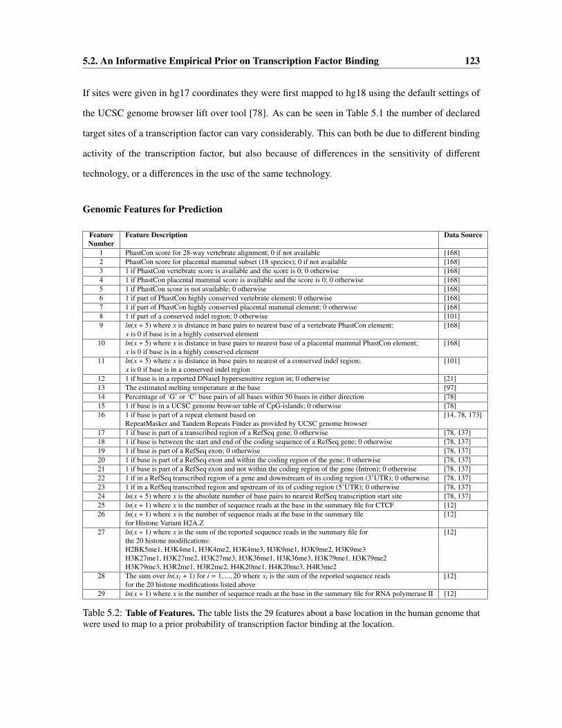
5.2. An Informative Empirical Prior on Transcription Factor Binding 123
If sites were given in hg17 coordinates they were first mapped to hg18 using the default settings of
the UCSC genome browser lift over tool [78]. As can be seen in Table 5.1 the number of declared
target sites of a transcription factor can vary considerably. This can both be due to different binding
activity of the transcription factor, but also because of differences in the sensitivity of different
technology, or a differences in the use of the same technology.
Genomic Features for Prediction
Feature Feature Description Data SourceNumber
1 PhastCon score for 28-way vertebrate alignment; 0 if not available [168]2 PhastCon score for placental mammal subset (18 species); 0 if not available [168]3 1 if PhastCon vertebrate score is available and the score is 0; 0 otherwise [168]4 1 if PhastCon placental mammal score is available and the score is 0; 0 otherwise [168]5 1 if PhastCon score is not available; 0 otherwise [168]6 1 if part of PhastCon highly conserved vertebrate element; 0 otherwise [168]7 1 if part of PhastCon highly conserved placental mammal element; 0 otherwise [168]8 1 if part of a conserved indel region; 0 otherwise [101]9 ln(x + 5) where x is distance in base pairs to nearest base of a vertebrate PhastCon element; [168]
x is 0 if base is in a highly conserved element10 ln(x + 5) where x is distance in base pairs to nearest base of a placental mammal PhastCon element; [168]
x is 0 if base is in a highly conserved element11 ln(x + 5) where x is distance in base pairs to nearest of a conserved indel region; [101]
x is 0 if base is in a conserved indel region12 1 if base is in a reported DNaseI hypersensitive region in; 0 otherwise [21]13 The estimated melting temperature at the base [97]14 Percentage of ‘G’ or ‘C’ base pairs of all bases within 50 bases in either direction [78]15 1 if base is in a UCSC genome browser table of CpG-islands; 0 otherwise [78]16 1 if base is part of a repeat element based on [14, 78, 173]
RepeatMasker and Tandem Repeats Finder as provided by UCSC genome browser17 1 if base is part of a transcribed region of a RefSeq gene; 0 otherwise [78, 137]18 1 if base is between the start and end of the coding sequence of a RefSeq gene; 0 otherwise [78, 137]19 1 if base is part of a RefSeq exon; 0 otherwise [78, 137]20 1 if base is part of a RefSeq exon and within the coding region of the gene; 0 otherwise [78, 137]21 1 if base is part of a RefSeq exon and not within the coding region of the gene (Intron); 0 otherwise [78, 137]22 1 if in a RefSeq transcribed region of a gene and downstream of its coding region (3’UTR); 0 otherwise [78, 137]23 1 if in a RefSeq transcribed region and upstream of its of coding region (5’UTR); 0 otherwise [78, 137]24 ln(x + 5) where x is the absolute number of base pairs to nearest RefSeq transcription start site [78, 137]25 ln(x + 1) where x is the number of sequence reads at the base in the summary file for CTCF [12]26 ln(x + 1) where x is the number of sequence reads at the base in the summary file [12]
for Histone Variant H2A.Z27 ln(x + 1) where x is the sum of the reported sequence reads in the summary file for [12]
the 20 histone modifications:H2BK5me1, H3K4me1, H3K4me2, H3K4me3, H3K9me1, H3K9me2, H3K9me3H3K27me1, H3K27me2, H3K27me3, H3K36me1, H3K36me3, H3K79me1, H3K79me2H3K79me3, H3R2me1, H3R2me2, H4K20me1, H4K20me3, H4R3me2
28 The sum over ln(xi + 1) for i = 1, ..., 20 where xi is the sum of the reported sequence reads [12]for the 20 histone modifications listed above
29 ln(x + 1) where x is the number of sequence reads at the base in the summary file for RNA polymerase II [12]
Table 5.2: Table of Features. The table lists the 29 features about a base location in the human genome thatwere used to map to a prior probability of transcription factor binding at the location.

124Chapter 5. Integrating Multiple Evidence Sources to Predict Transcription Factor Binding
across the Human Genome
In Table 5.2 we list the 29 features we used to learn a prior on transcription factor binding.
Before using the feature values with the logistic regression classifier the feature values were stan-
dardized. Standardization of feature values was done by subtracting the mean of the feature and
then dividing by its standard deviation.
The first 11 features all are related to conservation, and computed based on data obtained from
the UCSC Genome Browser site [78]. Features 1 and 2 are the PhastCon conservation [168] score
based on alignment of 28 vertebrate species and an 18 species placental mammal subset respectively.
The PhastCon method is based on a two-state Phloygenetic-HMM [168] and the score represents
the posterior probability that the hidden state is the conserved state at that base. For about 2% of
bases no PhastCon score was available, and in these cases we set the probability to 0. We note
that about 40% of bases have a PhastCon score of 0 in the provided files, with the next largest value
0.001. Since there might be a significant difference between PhastCon values of 0, and those slightly
greater than 0 we added three features related to PhastCon scores of 0. Features 3 and 4 are binary
features indicating if PhastCon score was available and 0, for the vertebrate and placental mammal
alignments respectively. Feature 5 was a binary feature indicating if the PhastCon score was not
available and thus set to 0, which was always the same for both vertebrate and the placental mam-
mal subset. The UCSC Genome Browser download site [78] also provides continuous stretches of
bases that are highly conserved based on the PhastCon score. Features 6 and 7 are binary features
indicating if the base fell within one of these PhastCon highly conserved element for the vertebrate
and the placental mammal subsets respectively. Feature 8 indicates if a base is in a region identified
as conserved based on a lack of indels, that is insertions or deletions of bases in sequences align-
ments with mouse and dog [101]. This measure does not take into account nucleotide substitutions
which drives the PhastCon scores. Features 9, 10 and 11 are the natural log of the number of bases to
the nearest base that is within a PhastCon highly conserved vertebrate element, PhastCon conserved
placental mammal, or indel conserved region after adding a pseudo-count of 5.
Feature 12 is a binary feature indicating if the base was in an experimentally determined DNaseI
hypersensitive regions in CD4+T cells [21]. DNaseI hypersensitive regions correlate with nucleo-
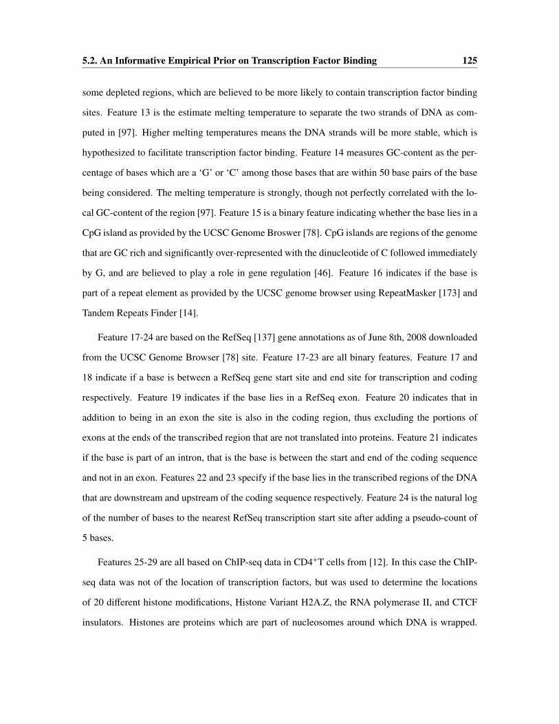
5.2. An Informative Empirical Prior on Transcription Factor Binding 125
some depleted regions, which are believed to be more likely to contain transcription factor binding
sites. Feature 13 is the estimate melting temperature to separate the two strands of DNA as com-
puted in [97]. Higher melting temperatures means the DNA strands will be more stable, which is
hypothesized to facilitate transcription factor binding. Feature 14 measures GC-content as the per-
centage of bases which are a ‘G’ or ‘C’ among those bases that are within 50 base pairs of the base
being considered. The melting temperature is strongly, though not perfectly correlated with the lo-
cal GC-content of the region [97]. Feature 15 is a binary feature indicating whether the base lies in a
CpG island as provided by the UCSC Genome Broswer [78]. CpG islands are regions of the genome
that are GC rich and significantly over-represented with the dinucleotide of C followed immediately
by G, and are believed to play a role in gene regulation [46]. Feature 16 indicates if the base is
part of a repeat element as provided by the UCSC genome browser using RepeatMasker [173] and
Tandem Repeats Finder [14].
Feature 17-24 are based on the RefSeq [137] gene annotations as of June 8th, 2008 downloaded
from the UCSC Genome Browser [78] site. Feature 17-23 are all binary features. Feature 17 and
18 indicate if a base is between a RefSeq gene start site and end site for transcription and coding
respectively. Feature 19 indicates if the base lies in a RefSeq exon. Feature 20 indicates that in
addition to being in an exon the site is also in the coding region, thus excluding the portions of
exons at the ends of the transcribed region that are not translated into proteins. Feature 21 indicates
if the base is part of an intron, that is the base is between the start and end of the coding sequence
and not in an exon. Features 22 and 23 specify if the base lies in the transcribed regions of the DNA
that are downstream and upstream of the coding sequence respectively. Feature 24 is the natural log
of the number of bases to the nearest RefSeq transcription start site after adding a pseudo-count of
5 bases.
Features 25-29 are all based on ChIP-seq data in CD4+T cells from [12]. In this case the ChIP-
seq data was not of the location of transcription factors, but was used to determine the locations
of 20 different histone modifications, Histone Variant H2A.Z, the RNA polymerase II, and CTCF
insulators. Histones are proteins which are part of nucleosomes around which DNA is wrapped.

126Chapter 5. Integrating Multiple Evidence Sources to Predict Transcription Factor Binding
across the Human Genome
Histones can be modified by the addition of certain chemical molecules. The different histone
modifications differ as to which histone of the nucleosome is targeted, which amino acid of the
histone is modified, and what molecule is added. H2A.Z is not a histone modification, but rather a
specific variant of one of the histone proteins that is part of a nucleosome. The RNA polymerase II
is a complex involved in transcribing DNA to RNA. A CTCF protein is involved in insulation, that
is it partitions the genome into domains of expression [195]. We used the summary data files from
the supporting website of [12] which provided the number of tags within a 200 base pair window for
all features except for the RNA polymerase and the CTCF insulator protein for which the number of
bases was 400. For the RNA polymerase, CTCF insulator, and H2A.Z we have a feature that is the
natural log of the number of tags plus one. The histone modification features, 27 and 28, are based
on 20 different histone modifications. Feature 27 is the natural log of the sum of the number of
tags for histone modifications across all 20 histone modification types. Feature 28 is the sum of the
natural log of histone modifications. We note for the same total number of histone tags, Feature 28
will be larger if the tags are distributed uniformly across all the different histone modification, while
for Feature 27 only the total number of tags matters and not how they are distributed. We chose
to combine the 20 histone modification values into these two features, instead of keeping each as
separate features, to avoid overfitting situations in which a specific histone modification is highly
predictive of binding for one transcription factor, but for which this modification does not generalize
to other transcription factors.
5.2.2 Results Using just the Prior
Illustrative Example
We first provide an illustrative example of the prior probabilities visualized in the UCSC Genome
Browser [78] as a custom track. We show here in (Figure 5.1 top) an example of the prior probability
of binding across a 250,000 base region along chromosome 20 of the human genome. Below the
plot of transcription factor binding probability prior are shown the location of RefSeq genes. In
this figure, five of the six tallest peaks are concentrated around RefSeq transcription start sites,

5.2. An Informative Empirical Prior on Transcription Factor Binding 127
Figure 5.1: Example of the empirical prior or transcription factor binding viewed using a custom track ofthe UCSC Genome Browser [78]. (Top) A 250,000 base pair region of chromosome 20 shows the learnedprior for transcription factor binding. Below the plot of the prior is shown the location of RefSeq genes.Most of the peaks in this image correspond to a RefSeq transcription start. (Middle) A zoomed in view ofthe peak circle in green in the top figure and labeled with the number 1, that is near the transcription start siteof C20orf24. We see from this image that the exons of C20orf24 have lower probability than its immediatesurrounding bases. (Bottom) A zoomed in view of the peak circle in red and labeled with a number 2 in thetop figure. This peak is not near a RefSeq transcription start, but there is other evidence supporting it such asbeing in a DNaseI Hypersensitive Region and containing a PhastCon conserved element.

128Chapter 5. Integrating Multiple Evidence Sources to Predict Transcription Factor Binding
across the Human Genome
for the genes TGIF2, SLA2, NDRG3, DSN1, and C20orf24. There is a smaller peak around the
transcription start site for the only other RefSeq gene transcription start site in the region, MYL9. In
Figure 5.1 (middle) we show a zoomed in view of a 6000 base pair region around the gene C20orf24,
circled in green in Figure 5.1 (top). For C20orf24 we note that the prior probability drops at the two
exons of the gene as compared to the immediate surrounding bases. We note that in Figure 5.1 (top)
there is peak, circled in red, that does not correspond to the transcription start site of a RefSeq gene
(a zoomed in view of this peak can be seen in Figure 5.1 (bottom)). However there is other evidence
supporting this location as containing a potential transcription factor binding site including it was
determined to be a DNaseI hypersensitive region in the experiments of [21] and contains a highly
conserved PhastCon element [168] using both the vertebrate and placental mammal alignments.
Cross-Validation Analysis
We are interested here in the question as to how well the prior could differentiate between a base
in a center of a region reported to be bound by a transcription factor and a randomly selected site,
without using any information about the binding motif of the transcription factor. For this evaluation
we tested on each of the 14 data sets listed in Table 5.1. The random bases were generated as
described above with 49 random sites for every real site. When testing on a data set we held it
out from training, along with any data set for the same transcription factor or data sets that was
published in the same paper as the data set being tested. We note that this evaluation task is both
more challenging and realistic than a cross-validation procedure that would hold out random subset
of locations from the full data keeping some positive examples from all data sets.
In Figure 5.2 we show the Receiver Operator Characteristic (ROC) curves in blue for each of
the 14 test cases. An ROC curve shows the false positive rate along the x-axis and the true positive
rate along the y-axis, as the threshold varies for declaring a prediction to be a real site. A perfect
ROC curve would be a horizontal line at one. The ROC curve expected from random guessing is
the diagonal y = x line shown in red.
A common metric to summarize an ROC curve is the area under the curve (AUC) value. A

5.2. An Informative Empirical Prior on Transcription Factor Binding 129
perfect AUC value is 1, while an AUC value of 0.5 is expected from random guessing. At the
bottom of Table 5.3 we show the AUC value for these data sets using our method. We also show
the AUC values that could be obtained just using any one feature. When there is a tie among sites
with the same feature value we randomly ordered the sites. We see that for 12 of the 14 data sets,
the AUC value for our method was greatest, and for the c-Myc data set it was tied with the feature
of the distance to the nearest transcription start site. This demonstrates the benefit of integrating
the various features we considered. In the last column of the table we summarize all these AUC
values by taking the average across all 14 data sets. Our method had the highest average AUC value
of 0.77, with the next highest average AUC values for the two features containing information on
histone modifications (0.72 and 0.71). The difference in AUC values between our method and the
top histone modification was statistically significant (p-value <10−4 based on a paired t-test). We
note that the AUC value is only a summary over all false positive rates, and does not imply for
instance that histone modifcations would be better than all other features at all false positive rates.
Also we note that these AUC values here do not measure the contribution of a feature when used in
conjunction with the other features.
The p53 data set was an outlier in that no feature could achieve an AUC value above 0.60, and
the cross-validation score was only 0.55. The p53 data set had the smallest number of detected
bound regions detected of any of the 14 experiments, so it is possible that there still are many p53
binding sites that would receive a high prior score, which were either not detected as bound or not
bound in the condition considered. A previous analysis of the bound p53 binding sites detected in
this experiment found an enrichment for p53 sites in Endogenous Retrovirus (ERV) retroelements,
and suggested using these elements as a mechanism by which p53 was able to propagate its binding
sites [187]. As ERVs are specific to the primate lineage and selected against being near genes [187],
this could also explain why the features we consider are less predictive of p53 binding sites.
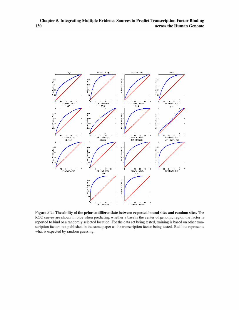
130Chapter 5. Integrating Multiple Evidence Sources to Predict Transcription Factor Binding
across the Human Genome
Figure 5.2: The ability of the prior to differentiate between reported bound sites and random sites. TheROC curves are shown in blue when predicting whether a base is the center of genomic region the factor isreported to bind or a randomly selected location. For the data set being tested, training is based on other tran-scription factors not published in the same paper as the transcription factor being tested. Red line representswhat is expected by random guessing.
5.2. An Informative Empirical Prior on Transcription Factor Binding 131
Feature c-Myc ERαc ERαp FoxA1 KAP1 RELA NRSF p53 p63+ p63− STAT1s STAT1u USF1 USF2 Average1. PhastCon Vertebrate 0.54 0.60 0.56 0.62 0.54 0.53 0.57 0.56i 0.58 0.57 0.56 0.56 0.55 0.53 0.552. PhastCon Placental 0.55 0.61 0.57 0.63 0.52 0.53 0.58 0.56i 0.58 0.58 0.57 0.57 0.55 0.53 0.563. Conservation Vertebrate Zero 0.53i 0.55i 0.54i 0.57i 0.53i 0.52i 0.54i 0.58 0.55i 0.55i 0.55i 0.56i 0.55i 0.52i 0.53i
4. Conservation Placental Zero 0.53i 0.56i 0.55i 0.58i 0.52i 0.52i 0.55i 0.58 0.56i 0.55i 0.55i 0.56i 0.54i 0.52i 0.54i
5. Missing Conservation Value 0.50i 0.50 0.50i 0.51i 0.51i 0.51i 0.51i 0.52 0.50i 0.50i 0.50i 0.52 0.52i 0.51i 0.50i
6. In PhastCon Vertebrate Elem. 0.53 0.56 0.52 0.56 0.53 0.51 0.53 0.51 0.53 0.53 0.53 0.54 0.51 0.53 0.537. In PhastCon Placental Elem. 0.53 0.57 0.53 0.56 0.51 0.51 0.54 0.52 0.54 0.53 0.54 0.55 0.51 0.53 0.548. In an Indel Conserved Elem. 0.53 0.58 0.53 0.58 0.53 0.51 0.55 0.52 0.54 0.55 0.54 0.55 0.52 0.54 0.549. Dist. to PhastCon Vertebrate Elem. 0.62i 0.69i 0.60i 0.71i 0.63i 0.57i 0.71i 0.51i 0.65i 0.66i 0.68i 0.69i 0.69i 0.74i 0.65i
10. Dist. to PhastCon Placental Elem. 0.63i 0.70i 0.61i 0.72i 0.56i 0.58i 0.71i 0.50i 0.66i 0.66i 0.68i 0.70i 0.69i 0.74i 0.65i
11. Dist. to Indel Conserved Elem. 0.60i 0.68i 0.60i 0.70i 0.59i 0.56i 0.67i 0.51 0.65i 0.65i 0.63i 0.63i 0.64i 0.68i 0.63i
12. In DNaseI Hypersensitive Region 0.61 0.54 0.51 0.53 0.54 0.54 0.55 0.54 0.55 0.55 0.64 0.71 0.71 0.77 0.5913. Melting Temperature 0.70 0.70 0.60 0.55 0.70 0.62 0.74 0.60 0.56 0.62 0.67 0.73 0.75 0.76 0.6614. GC Ratio 0.69 0.68 0.58 0.54 0.67 0.61 0.74 0.58 0.55 0.60 0.66 0.72 0.72 0.72 0.6515. In CpG Island 0.58 0.52 0.50i 0.50 0.51 0.52 0.55 0.53 0.50 0.51 0.56 0.60 0.56 0.57 0.5416. In Repeat 0.59i 0.71i 0.60i 0.71i 0.64i 0.55i 0.67i 0.54 0.71i 0.71i 0.64i 0.64i 0.69i 0.71i 0.65i
17. In Transcribed Region 0.57 0.54 0.51i 0.54 0.50 0.52 0.52 0.51 0.54 0.54 0.51 0.50i 0.52 0.50 0.5318. In Coding Region 0.53 0.52 0.51i 0.53 0.51i 0.50 0.51i 0.51 0.52 0.53 0.51i 0.54i 0.53i 0.55i 0.50i
19. In Exon 0.52 0.51 0.50i 0.50 0.51 0.50 0.52 0.52 0.51 0.51 0.51 0.52 0.50 0.52 0.5120. In Exon and Coding Region 0.51 0.52 0.50i 0.50 0.51 0.50i 0.51 0.52 0.51 0.51 0.50 0.50 0.50i 0.50 0.5121. In Intron 0.52 0.52 0.50i 0.53 0.53i 0.50i 0.51i 0.51 0.53 0.53 0.51i 0.54i 0.53i 0.55i 0.50i
22. In 3’ UTR 0.50 0.51 0.50i 0.50 0.50i 0.50i 0.51 0.52 0.50 0.51 0.50 0.50i 0.51i 0.50i 0.5023. In 5’ UTR 0.54 0.53 0.50i 0.51 0.51 0.51 0.53 0.52 0.53 0.52 0.53 0.53 0.54 0.56 0.5324. Distance to Nearest TSS 0.74i 0.59i 0.53i 0.56i 0.62i 0.59i 0.61i 0.55i 0.61i 0.62i 0.67i 0.69i 0.83i 0.81i 0.64i
25. Log of Number of CTCF Tags 0.61 0.57 0.53 0.55 0.52 0.55 0.57 0.54 0.54 0.54 0.68 0.77 0.65 0.70 0.5926. Log of Number of H2A.Z Tags 0.62 0.58 0.54 0.58 0.55 0.56 0.52 0.57 0.57 0.58 0.67 0.73 0.73 0.79 0.6127. Log of Sum of Histone Tags 0.73 0.75 0.64 0.68 0.67 0.65 0.77 0.59 0.64 0.67 0.75 0.82 0.83 0.82 0.7228. Sum of Log of Histone Tags 0.72 0.75 0.64 0.68 0.66 0.64 0.77 0.58 0.64 0.67 0.74 0.80 0.81 0.81 0.7129. Log of RNA Polymerase Tags 0.66 0.57 0.54 0.56 0.53 0.57 0.57 0.53 0.57 0.57 0.67 0.76 0.73 0.78 0.62
Cross-Validation 0.74 0.84 0.68 0.78 0.73 0.66 0.82 0.55 0.74 0.77 0.81 0.87 0.90 0.90 0.77
Table 5.3: Comparison of the Prior with Individual Features. The table shows the AUC values that canbe obtained when using each feature individually, and at the bottom when integrating the data sources. Bothranking sites by the feature in increasing and decreasing order was considered with the larger value shown. Ifthere is a superscript i after the AUC value, then a larger AUC value was obtained when the sites were rankedin increasing order of the feature. Ties in values were broken randomly. The highest value in each column isin bold, while the second highest is in italics. For 13 of the 14 data sets the AUC value of the cross-validationscore is in bold. The last column is the average AUC value for the feature over all data sets, where all sitesmust be consistently ranked by the feature in either increasing or decreasing order, whichever gave a higherAUC value.

132Chapter 5. Integrating Multiple Evidence Sources to Predict Transcription Factor Binding
across the Human Genome
5.3 Combining the Prior with Motif Information
In the previous section we discussed a method to obtain an empirical prior probability that a tran-
scription factor would bind each base in the genome based on general features not specific to the
transcription factor. In this section we discuss how this prior can be combined with motif informa-
tion for a specific transcription factor to predict which regions of the genome are more likely to be
bound by the transcription factor.
5.3.1 Method for Combining the Prior with Motif Evidence
We assume here we have a set of regions for which we like to know which ones the transcription
factor would most likely bind. A region contains L continuous base locations, ba, ..., ba+L−1. We
assume L is either the same or at least reasonably similar for different regions. Associated with each
location is the prior which we will denote p(bi) that base bi is bound by a transcription factor, that
is p(bi) = P(bi| fbi) as defined in the last section. For base bi we also have a motif score for the site
on the positive strand that begins at position bi, which we will denote m+(bi) and a motif score for
the site on the negative strand which ends at base bi denoted m−(bi).
For the results in this section we represented the motif with a positional weight matrix (PWM)
and the score was computed using a zero order background model (see Chapter 1 and [50]). The
nucleotide probabilities were set to their genome-wide proportion. A pseudo-count of twice its
genome-wide proportion was added to each entry in the PWM. In our results the scores for m+(bi)
and m−(bi) were defined as
m+(bi) =
∏W−1j=0 θpwm j+1(g+(bi+ j))∏W−1
j=0 θbackground(g+(bi+ j))(5.1)
m−(bi) =
∏W−1j=0 θpwm j+1(g−(bi+W− j−1))∏W−1
j=0 θbackground(g−(bi+W− j−1))(5.2)
where g+(x) and g−(x) represent the nucleotides on the positive and negative strands at location x
respectively. θbackground(y) is the background probability of nucleotide y. θpwm j(y) is the probability

5.3. Combining the Prior with Motif Information 133
the PWM model gives at position j of observing nucleotide y where the PWM is indexed starting at
position 1.
The motif score we associate with base bi is
m(bi) = max(m+(bi),m−(bi)) (5.3)
For a motif of length W we defined a combined prior and motif score at each location bi as
s(bi) = m(bi) ×1W
W∑j=1
p(b j+i) (5.4)
Here we are averaging the prior score over each base position of the potential binding site. Now
to score the entire region of length L we will consider two methods to combine the motif and prior
score. One method takes the maximum value of s(bi) in the region while the other takes its average
value. These two formula are written below.
maxMOT IF×PRIOR = max(s(b1), ..., s(bL)) (5.5)
avgMOT IF×PRIOR =1L
L∑i=1
(s(bi)) (5.6)
In the results section for comparison purposes we will consider three simpler strategies defined
below. maxMOT IF is the maximum motif score at any site in the region. avgMOT IF is the average
motif score in the region, which has been suggested previously [44]. avgPRIOR is the average prior
score in the region. Formally these are written
maxMOT IF = max(m(b1), ...,m(bL)) (5.7)
avgMOT IF =1L
L∑i=1
m(bi) (5.8)
avgPRIOR =1L
L∑i=1
p(bi) (5.9)

134Chapter 5. Integrating Multiple Evidence Sources to Predict Transcription Factor Binding
across the Human Genome
5.3.2 Results for Combining the Prior with Motif Information
In this sub-section we will present results on combining the prior with a motif. We will first present
results using cross-validation with the data sets we have been training. We will then presents results
on an independent set of promoter ChIP-chip data which we had not been using at all for training.
Cross-Validation Analysis
Regulator Motif ID Motif Accessionp53 V$P53 01 M00034NRSF V$NRSF Q4 M01028USF1 V$USF Q6 01 M00796USF2 V$USF Q6 01 M00796p63 V$P53 DECAMER Q2 M00761c-Myc V$MYC Q2 M00799STAT1 V$STAT 01 M00223FoxA1 V$HNF3ALPHA Q6 M00724ERα V$ER Q6 M00191RELA V$NFKAPPAB 01 M00054
Table 5.4: Table of Motifs. This table provides the identifying information for the motifs from the TRANS-FAC database that we used in the analysis.
We are interested here in the following question: given the prior and a motif for a transcrip-
tion factor of interest to what extent could a method predict which genes would have a reported
center of bound region of this transcription factor within 10,000 bases of its transcription start
site. We made ranked predictions for all 21,257 RefSeq transcription start sites. Such a set of
regions are of interest, since predicted binding sites for the transcription factor in these regions
could then be used to associate the transcription factor with regulating the gene corresponding to
the start site. For evaluation we used 13 of the 14 data sets used in the Section 5.2.2, using the
same cross-validation procedure on data sets described there. We excluded the KAP1 data set since
it a co-repressor and does not have a motif itself. Table 5.4 lists the motifs from the TRANS-
FAC databases we used to compute the PWM score. In Figure 5.3 we present the ROC curves
comparing the maxMOT IF , avgMOT IF , avgPRIOR, maxMOT IF×PRIOR, and avgMOT IF×PRIOR methods
described above. These charts are summarized with AUC values in Table 5.5. In the last row of
this table we average the AUC over all data sets considered. We see that on average the AUC with

5.3. Combining the Prior with Motif Information 135
Figure 5.3: ROC Curves for Identifying Promoter Regions Bound by a Transcription Factor. Here wecompare on 13 data sets 6 methods to prediction whether a transcription start site will have the transcriptionfactor reported to bind within 10,000 bases.

136Chapter 5. Integrating Multiple Evidence Sources to Predict Transcription Factor Binding
across the Human Genome
either the maxMOT IF×PRIOR or avgMOT IF×PRIOR method is greater than the maxMOT IF , avgMOT IF ,
and avgPRIOR methods. The difference between the avgMOT IF×PRIOR and avgMOT IF methods had a
p-value <0.001, while the difference between the avgMOT IF×PRIOR and avgPRIOR methods had a p-
value of 0.03, both of which are based on paired t-tests. We did not observe a significant difference
between using the maxMOT IF×PRIOR and avgMOT IF×PRIOR in our results.
In Figure 5.3 we also compare with ranking each region based on the highest scoring site on
the UCSC TFBS conserved track [78] for the transcription factor (pink line in Figure 5.3). As men-
tioned above, for a site to be on the UCSC TFBS conserved track the site must pass a threshold for
conservation in mouse and rat, but there is no restriction in terms of its distance to the transcription
start site. The score for the transcription factor was used as provided by the UCSC genome browser
so in some cases it used slightly different motifs for the transcription factor than we used. No predic-
tions for FoxA1 and p63 were available from the UCSC TFBS conserved track. Also some regions
did not have any site reported, either because it did not meet their minimum score threshold or was
not conserved, which is why its ROC curve does not reach a true positive rate of 1. This is also why
we did not include this method in the comparison in Table 5.5. In no case did we observe the curves
based on the UCSC track dominate either the maxMOT IF×PRIOR, or averageMOT IF×PRIOR curves. In
cases such as c-Myc, NRSF, and p53 the predictions based on the UCSC TFBS conserved track
were inferior in our evaluation.
Evaluation on E2F Promoter ChIP-chip Data
We next evaluated the ability of the prior to improve prediction of targets of the E2F family of
transcription factors identified based on extensive ChIP-chip experiments [196]. The ChIP-chip ex-
periments were conducted on promoter arrays with approximately 1500 bases for a promoter [196].
As E2F was not a transcription factor for which genome-wide coverage of its binding was available,
we did not use it in learning the prior. We note that some of the promoters in this data set are not
represented with an annotated RefSeq transcription site, unlike for the regions used for the previ-
ous results. In total the data set of [196] contained 30 ChIP-chip experiments for the transcription

5.3. Combining the Prior with Motif Information 137
Figure 5.4: Results at Predicting Targets of the E2F Family of Transcription Factors. The chart showsa comparison of five methods for the task of predicting gene targets of the E2F family of transcription factorsbased on 30 different ChIP-chip experiments. For each method, an AUC value was computed for each of the30 experiments. The 30 AUC values for a method were then ordered in descending order. The x-axis showsthe position in this ordering, and the y-axis shows the AUC value corresponding to the position. The plotshows that the methods that use jointly the prior and motif have a higher AUC value at each rank positionthan methods that only use the prior or only the motif information, thus performing better in our evaluation.The results also show that the method just based on the prior had higher AUC values than the methods basedjust on the motif information.

138Chapter 5. Integrating Multiple Evidence Sources to Predict Transcription Factor Binding
across the Human Genome
Data Set Max Average Average Max (Prior× Average (Prior×PWM Score PWM Score Prior PWM Score) PWM Score)
c-Myc 0.54 0.60 0.69 0.66 0.68ERαc 0.59 0.63 0.62 0.64 0.67ERαp 0.64 0.64 0.56 0.64 0.65FoxA1 0.52 0.52 0.59 0.61 0.64RELA 0.57 0.59 0.64 0.62 0.63NRSF 0.83 0.83 0.54 0.83 0.83
p53 0.82 0.82 0.56 0.80 0.80p63+ 0.53 0.50 0.58 0.57 0.57p63− 0.53 0.54 0.59 0.58 0.58
STAT1s 0.53 0.51 0.74 0.66 0.71STAT1u 0.51 0.48 0.70 0.62 0.66USF1 0.69 0.67 0.68 0.81 0.78USF2 0.67 0.63 0.69 0.78 0.75
Average 0.61 0.61 0.63 0.68 0.69
Table 5.5: Table of AUC Values for Predicting if a RefSeq Transcription Start Site will have a Tran-scription Factor binding within 10,000 bases. The highest value in each row is shown in bold, while thesecond highest is shown in italics. In the bottom row we show the average AUC values for all 13 test cases.On average using both the prior and motif information outperformed either alone.
factors E2F1, E2F4, and E2F6 in 5 cell types: MCF10A, HelaS3, GM06990, Ntera2, and MCF7,
with two replicates for each of the fifteen combinations of transcription factor and cell type. For
each of the 30 ChIP-chip experiments we declared the bound targets of the transcription factor to be
those with an enrichment score >1 as defined and suggested in [196]. For each of the five methods
we considered we applied all the methods to only the portion of the genome that the probes on the
microarray cover, after converting the annotated hg17 coordinates to hg18 coordinates. We used the
E2F motif in the JASPAR database that has the ID MA0024. We computed the AUC values for each
method in each experiment for the task of predicted the declared targets in the experiment. We then
for each method sorted in ranked order the AUC values across the 30 experiments, and plotted these
results in Figure 5.4. Here we see using the average value of the prior at each base in the region
out performs either the maximum or average motif score. When combining the prior with the motif
score we see an even greater improvement.
5.4 Discussion
In this chapter we presented a method that leveraged recent genome-wide data sets to learn a prior
on transcription factor binding across the human genome. We showed that a method that integrates

5.4. Discussion 139
a variety of data sources could better predict if a location in the genome would be reported as bound
by a transcription factor than any one feature that we considered. Of the features we considered
the most informative single feature we used was based on experimentally determined locations
of histone modifications [12]. We then combined the prior with motif information for specific
transcription factors to predict whether regions within 10,000 base pairs of a transcription start site
would contain a reported binding site for the transcription factor. We also evaluated on additional
set of 30 E2F ChIP-chip experiments. We showed that by combining the motif score with the prior
score we could outperform using either alone. We compared both using the average and maximum
score given to each site based on the prior and PWM in the region, but could not conclude that either
using the average or maximum was better. We also compared to a method that filtered sites that did
not show evidence of conservation in mouse and rat, which gave worse results in our analysis,
indicating that this conservation requirement can cause true sites to be missed that could otherwise
be identified.
An interesting result was how effective the prior alone without any motif information could be
at predicting which promoter regions would be bound by the transcription factors we looked at.
One possible explanation for this is that values for some of the features that we used to form the
prior are predictive that the nearby gene is likely to be transcriptionally active (e.g. hypersensitivity
and histone modification features), and that transcriptionally active genes are more likely to have
transcription factors binding in its promoter region. As genes can encode proteins with very dif-
ferent functions, some of which are core functions, while others are more specialized, it should be
expected that genes will have a range of transcriptional activity levels. The prior might potentially
be identifying genes that are more likely to be transcriptionally active and need more transcription
factors to bind the promoter region to maintain the higher activity level.
The lowest AUC values we reported in Table 5.5 were for the two p63 data sets. As the motif dis-
covered using de-novo motif discovery using targets identified in the p63 genome-wide ChIP-chip
data [197] only weakly corresponds to the TRANSFAC motif these results are not too surprising.
Other papers have also reported improvements over the canonical motif for various transcription
140Chapter 5. Integrating Multiple Evidence Sources to Predict Transcription Factor Binding
across the Human Genome
factors using de-novo motif discovery on the bound targets [73, 188, 196]. It will be interesting
to see if the performance improves when using new experimentally determined motifs [15, 121] as
opposed to the curated TRANSFAC and JASPAR motifs.
Both the DNaseI hypersensitivity data [21] and the histone modifications [12] data sets were
based on CD4+T cells. We applied these features in predicting transcription factor binding across a
variety of different cell types. Even though the features were not collected in the same cell type the
transcription factor binding was measured, we showed that these features can still be informative.
As DNaseI hypersensitivity and histone modification data are collected in more cell types it will
be interesting to see to what extent predictions can be improved even further with this additional
data. It will also be interesting to see to what extent predictions can be improved even further by
bringing in addition data sets, such a recent genome-wide data set on nucleosome positioning [161].
As more experimental data sets on transcription factors binding locations become available, not
only could this be used as additional training data, but it could also be used as informative features
as well. Since it is reasonable to expect that transcription factors will be more likely bind where
other transcription factors are nearby. The interaction between transcription factors could also be
modeled by considering multiple motifs at a time, instead of considering each motif independently
as we are now, which has been shown to improve inference of targets of transcription factors [171].
The focus of our evaluation in this chapter was on the rankings produced by the various meth-
ods considering each transcription factor separately. It will also be interesting to explore if we can
predict how many sites a transcription factor binds. For instance one approach would be to look for
sites which have significantly higher scores than would be expected to be observed when randomiz-
ing columns of the PWM. However to effectively evaluate these types of approaches we will likely
need more data for transcription factors collected under more consistent procedures.
To apply the method to generate transcription factor-gene interactions for DREM, one must first
associate with each gene a region of the genome such that if the transcription factor binds there it
will be predicted to regulate the gene. These regions could be regions of the genome that are within
10,000 base pairs of a transcription start site, for which we presented results here, though other ways

5.4. Discussion 141
of defining the regions could be used as well. We note that while the choice of regions will effect
the transcription factor-gene interaction predictions, we expect that because of the prior, our method
will be more robust to this choice than a method that gives equal consideration to every base in a
region. Once regions of the genome are defined to be associated with genes, the method will provide
a ranking for each gene in terms of being a target of the transcription factor where we associate a
PWM with each transcription factor. We would then need to decide on a cutoff for each PWM.
One approach would be to simply take the top K ranking targets for each PWM. Another approach
would be to have different thresholds for different PWMs based for instance on comparing scores
obtained using the real PWM to those obtained when using randomized versions of the PWM. As
future work it would be useful to also consider the confidence in our predictions of transcription
factor-gene interactions as part of the input into DREM.
This chapter presented a method to improve the inference of transcription factor binding across
the human genome and for associating transcription factors with genes based on genomic properties.
As more data becomes available the predictions the method makes should be expected to improve
further. Such predictions when combined with time series gene expression data using methods
such as DREM have the potential to lead to important insights into transcription factors controlling
specific dynamic regulatory responses in human cells.


Chapter 6
Conclusions and Future Work
The main objective of this thesis has been to develop computational methods to allow better anal-
ysis and modeling of transcriptional gene regulation dynamics. We approached this problem from
three related directions. Our first direction was to develop a method that could identify statistically
significant temporal expression patterns in most time series gene expression data sets. We then fo-
cused on a method that explicitly modeled gene regulation dynamics by integrating time series gene
expression data and static transcription factor-gene association data. As genome-wide transcription
factor-gene association data is often not available experimentally, we then focused on developing
computational methods that could better predict transcription factor-gene associations, one of the
methods was motivated by E. coli and the other by human genomic data.
In Section 6.1 of this chapter we summarize the contributions presented in this thesis and some
conclusions reached. We end this chapter with a discussion of possible future extensions of the
work presented here (Section 6.2).
6.1 Conclusions
The first computational method we presented in this thesis was able to identify statistically signifi-
cant temporal expression profiles in short time series microarray expression data (Chapter 2). As we
143

144 Chapter 6. Conclusions and Future Work
discussed short time series expression experiments represent the majority of time series expression
experiments and a significant portion of all microarray experiments. However many prior methods
applied to analyze time series expression data either did not take advantage of the temporal ordering
of time points or were designed for longer time series. Our method by defining a set of distinct
profiles independent of the data, assigning genes to these profiles, and then using a permutation
test on the time points could detect if there was a statistical enrichment of genes assigned to a pro-
file. We showed on both simulated data and on a biological data set pertaining to human immune
response that the method effectively identified significant temporal expression patterns. We imple-
mented the method as part of the software the Short Time-series Expression Miner (STEM) which
has been downloaded by over 1000 researchers, and results obtained by others using the software
have appeared in a variety of biological journals.
While the STEM clustering method we presented in Chapter 2 is useful for analyzing short time
series expression data and directly applicable to a species even if transcription factor-gene inter-
action data is not available, there was two characteristics of the method that motivated us to also
propose the Dynamic Regulatory Events Miner (DREM) method for analyzing and modeling gene
regulation dynamics. The first characteristic is that the STEM method considered each temporal
expression pattern independently, while in reality these profiles can be related to each other tempo-
rally. For instance one would expect there often to be sets of genes that have the same expression
distribution until some point in time, and then diverge into two different temporal patterns. STEM
would not be able to model that genes of two different temporal profiles shared a common expres-
sion profile up until some time point. The second reason is that the STEM clustering method only
uses information from time series expression data, thus not taking advantage of important com-
plementary information on gene regulation available from transcription factor-gene interaction data
when available. The DREM method we proposed in Chapter 3 addressed these issues by mod-
eling the observed temporal expression patterns as a series of bifurcation of events controlled by
transcription factors. We based our model on a specific instance of an Input-Output Hidden Markov
Model (IOHMM), where the static transcription factor-gene interaction data is viewed as controlling
6.1. Conclusions 145
transitions between states, and each state has a time series expression level associated with it. We
applied the method to study stress response in yeast, using as input ChIP-chip data and time series
expression data. The method led to new experimentally validated predictions about yeast response
to stress.
The DREM method assumes the availability of transcription factor-gene interaction data. While
this data on a genome-wide scale is readily available in yeast, for most other organisms such data
is limited. We addressed this issue for E. coli in Chapter 4 by presenting a method that could
computationally predict transcription factor-gene interactions by leveraging validated targets of the
transcription factor, gene expression data, and a DNA binding motif information to predict addi-
tional gene targets. We discussed that for most genes it is not known whether they are regulated or
not by the transcription factor, but by taking a semi-supervised learning approach with these data
sources we could improve predictions over other methods previously suggested for the task. We
also show that the method could accurately discriminate between genes likely to be activated or re-
pressed targets of the transcription factor. We demonstrated the application of our predictions with
DREM on a new time series expression data set for the aerobic-anaerobic shift in E. coli.
In Chapter 5, we presented a method that for a human transcription factor could predict which
regions of the genome it was most likely to bind. The method only assumed the the availability of
a binding motif for the transcription factor. The method integrated a variety of genomic features
using a logistic regression classifier to form a probabilistic prior on transcription factor binding at
each base in the genome. To train the classifier we used recent genome-wide binding data sets for
a number of transcription factors. We demonstrated that the prior could better predict transcription
factor binding than any one feature on which the prior was based. We then demonstrated that
by combining the prior with motif information we could better predict which gene promoters a
specific transcription factor would bind, than when using the prior or motif information alone. These
predictions could then form the basis of the transcription factor-gene input used by DREM.
The methods we have presented here have enabled the improved analysis and modeling gene
regulation dynamics. We demonstrated with DREM that even when we did not have dynamic exper-

146 Chapter 6. Conclusions and Future Work
imental information on transcription factor-gene interactions, that by integrating experimental data
from one time point or static computational predictions with time series expression data, we could
still improve the modeling of a dynamical systems. The integration of temporal data with com-
plementary static sources is a more general computational problem that will likely be relevant in a
number of biological contexes. As biological systems are dynamic entities that constantly change
over time, computational models of these systems that do not account for time will only provide a
limited view on these systems. By explicitly considering time as we have done in this thesis one can
obtain a more accurate view of activity in biological systems.
6.2 Future Work
A number of future research directions extending the work presented in this thesis are possible. In
this section we will discuss some of them.
Modeling Additional Mechanisms of Gene Regulation
In the future it will be interesting to extend the dynamic models of gene regulation we presented here
to include mechanisms besides transcriptional regulation. While transcriptional gene regulation is
a major aspect of gene regulation, it is not the only aspect. For instance it will be interesting to
include in the models post-transcriptional regulation of the mRNA transcripts, which can determine
if a transcript will be translated into protein or will be degraded. MicroRNAs and proteins binding to
the transcript, particularly downstream of the protein coding region (3’ UTR), can enable this type
of regulation [132, 194]. Specific mRNA targets of these regulators can be inferred using either
computational methods [91, 194] or experimental methods such as RNA-chip [77]. One direct
approach to use these inferred interactions with DREM is to apply them as input in the same way
the transcription factor-gene interaction data is currently being used.
It will also be interesting to bring in data on post-translational regulation of transcription factors
for instance through phosphorylation, which might cause a transcription factor already existing in
6.2. Future Work 147
the cell in protein form to begin to regulate its target genes. Data from global surveys of phos-
phorylation [138] are beginning to make modeling this type of regulation feasible. Additionally
high-throughput data on protein-protein interactions [49, 85] could potentially make it possible to
model some signaling cascade scenarios, for instance a stimulus triggers a chain of interacting pro-
teins ending with a phosphorylation event that causes a transcription factor to become active. These
predictions of active transcription factors could then be linked with DREM providing evidence sup-
porting certain sets of transcription factors being active. If at the network level we have evidence
that an active transcription factor is more likely to be transcriptionally regulated as opposed to post-
transcriptionally regulated, then we would expect to observe an increase in its mRNA expression
level. DREM does not currently directly use the expression level of a transcription factor instead
using indirect evidence through the expression level of its target genes. Recent work is beginning
to suggest benefits from models that jointly consider the mRNA expression levels of a transcription
factor with the expression level of its predicted targets [166].
Modeling the Effects of Combinatorial Interactions on Gene Regulation
Combinatorial interactions among transcription factors can influence gene expression, and are par-
ticularly important in higher organisms [90]. DREM uses a logistic regression classifier to map the
set of transcription factor associated with regulating a gene to transition probabilities among states
in the model. As a logistic regression classifier can only learn linearly separable functions of its
inputs, the representation power of the logistic regression classifier is not sufficient to model all
combinatorial interactions of transcription factors as we are currently encoded the input. In order to
capture additional combinatorial interactions one could include additional features with the logistic
regression classifier. One such strategy would be to add additional features for pairs of transcription
factors. For instance if IA and IB are binary features indicating that transcription factors A and B
regulate the gene respectively, then if the feature min(IA, IB) is also provided to the classifier the
classifier would have sufficient representation power to model OR, AND, and XOR regulation logic
for the pair [18]. One issue with this approach is that the number of pairs of transcription factors

148 Chapter 6. Conclusions and Future Work
grows quadratically with the number of input transcription factors and thus it will not be realistic
to consider all pairs. One way to deal with this issue would be to only add a feature for a pair if
there is a significant intersection in the genes regulated by the two transcription factors. Another
strategy instead of explicitly adding additional features, would be to use a logistic regression classi-
fier based on kernels, which would enable the classifier to consider higher order interaction features
implicitly [84].
Incorporating de Novo Motif Discovery into DREM
Currently DREM is limited to using transcription factors which are provided in the input. De novo
motif discovery allows the discovery of latent features for transcription factors not included in the
input. De novo motif discovery works by attempting to discover a common binding motif in an input
set of sequences that are related, for instance these sequences could all be promoter regions of genes
assigned to the same path in DREM. The problem of de novo motif discovery has received extensive
attention in the literature based on a variety of approaches including Gibbs Sampling [87, 98, 150],
Expectation-Maximization [5], and dictionary approaches [130]. A review of a number of methods
and a comparative evaluation can be found in [179]. The results of [179] indicate that motif dis-
covery problem is a challenging problem particularly in higher organisms. One potential avenue for
improving motif discovery is to use priors such as the one we derived in Chapter 5 to guide the motif
discovery to place greater emphasis on sites with a higher prior. Such a strategy where the prior was
based on only nucleosome positioning in yeast was shown to improve motif discovery [118].
Improving Further the Prediction of Transcription Factor-Gene Interactions
While the methods we have presented in Chapters 4 and 5 can be used to improve the prediction
of transcription factor-gene interactions there remains substantial room for improvement. To some
extent we expect improvement to be enabled by new data sources that will provide more experi-
mentally confirmed binding sites, more accurate transcription factor binding motifs, and additional
features to form even more informative priors. Computationally we could potentially improve our
prediction of targets of transcription factors by extending the methods we presented to jointly con-

6.2. Future Work 149
sidering multiple transcription factors at a time. The methods we presented were designed to pre-
dict targets of a transcription factor making no assumption about the availability of high-throughput
ChIP based data for the transcription factor. In the future as more factors have high-throughput
ChIP based data available in at least one condition, it will be interesting to extend the methods we
presented to also leverage this data when predicting targets of the transcription factor in other con-
ditions.
Applying the Methods to Additional Organisms
In order to apply DREM to an organism of interest it is necessary to have transcription factor-gene
interaction input for the organism. In this thesis we have presented computational methods to pre-
dict transcription factor-gene interactions in E. coli and human. However we expect there will be
interest in applying DREM to other model organisms such as mouse, rat, fly, and the plant Ara-
bidopsis thaliana. Depending on the available data for the organisms the methods we presented
might be directly applicable, or may need to be extended. For the method we used for E. coli
(Chapter 4) having confirmed targets of the transcription factor was necessary. For the method we
applied to human data (Chapter 5) having a binding motif for the transcription factor, as well as
informative features and sufficient training data to learn a prior on transcription factor binding was
necessary. Ideally the availability of these predicted transcription factor-gene interactions would
lead researchers to combine them with time series expression data of interest in DREM leading
to new biological hypothesis being formed, that could be followed up with additional biological
experiments. For instance DREM can lead to predictions that specific transcription factors are reg-
ulating specific sets of genes in specific conditions at specific time points. As demonstrated in
Chapter 3, these type of predictions can be followed up with Chromatin Immunoprecipitation based
experiments. Microarray experiments of cells subjected to genetic deletion [67] or RNAi interfer-
ence [184] of the transcription factor can be used to validate its predicted functional importance
when a predicted set of genes it regulates shows a difference in expression level as compared to in
wild type cells.


Bibliography
[1] S. Alexeeva, K.J. Hellingwerf, and M.J. Teixeira de Mattos. Requirement of ArcA for redox
regulation in Escherichia coli under microaerobic but not anaerobic or aerobic conditions. J
Bacteriol, 185:204–209, 2003.
[2] M.N. Arbeitman, E.E. Furlong, F.J. Imam, E. Johnson, B.H. Null, B.S. Baker, M.A. Krasnow,
M.P. Scott, R.W. Davis, and K.P. White. Gene expression during the life cycle of Drosophila
melanogaster. Science, 298:2270–2275, 2002.
[3] M. Ashburner, C.A. Ball, J.A. Blake, D Botstein, H. Butler, J.M. Cherry, A.P. Davis,
K. Dolinski, S.S. Dwight, J.T. Eppig, M.A. Harris, D.P. Hill, L. Issel-Tarver, A. Kasarskis,
S. Lewis, J.C. Matese, J.E. Richardson, M. Ringwald, G.M. Rubin, and G. Sherlock. Gene
Ontology: tool for the unification of biology. Nat Genet, 25:25–29, 2000.
[4] M.M. Babu and S.A. Teichmann. Functional determinants of transcription factors in Es-
cherichia coli: protein families and binding sites. Trends Genet, 19:75–79, 2003.
[5] T.L. Bailey and C. Elkan. Fitting a mixture model by expectation maximization to discover
motifs in biopolymers. In Proceedings of the Second International Conference on Intelligent
Systems for Molecular Biology, pages 873–880, 1994.
[6] R.E. Baker and D.C. Masison. Isolation of the gene encoding the Saccharomyces cerevisiae
centromere-binding protein CP1. Mol Cell Biol, 10:2458–2467, 1990.
151

152 BIBLIOGRAPHY
[7] G. Balazsi, A. Barabasi, and Z.N. Oltvai. Topological units of environmental signal process-
ing in the transcriptional regulatory network of Escherichia coli. Proc Natl Acad Sci USA,
102:7841–7846, 2005.
[8] Z. Bar-Joseph, G. Gerber, D. Gifford, T. Jaakkola, and I. Simon. Continuous representations
of time series gene expression data. J Comput Biol, 10:341–356, 2003.
[9] Z. Bar-Joseph, G.K. Gerber, T.I. Lee, N.J. Rinaldi, J.Y. Yoo, F. Robert, D.B. Gordon,
E. Fraenkel, T.S. Jaakkola, R.A. Young, and D.K. Gifford. Computational discovery of gene
modules and regulatory networks. Nat Biotech, 21:1337–1342, 2003.
[10] A. Barabasi and Z.N. Oltvai. Network biology: understanding the cell’s functional organiza-
tion. Nat Rev Genet, 5:101–113, 2004.
[11] T. Barrett, T. O. Suzek, D. B. Troup, S. E. Wilhite, W. C. Ngau, P Ledoux, D Rudnev,
A. E. Lash, W Fujibuchi, and R Edgar. NCBI GEO: mining millions of expression profiles-
database and tools. Nucleic Acids Res, 33:D562–D566, 2005.
[12] A. Barski, S. Cuddapah, K. Cui, T.Y. Roh, D.E. Schones, Z. Wang, G. Wei, I. Chepelev,
and K. Zhao. High-resolution profiling of histone methylations in the human genome. Cell,
129:823–837, 2007.
[13] Y. Bengio and P. Frasconi. An Input Output HMM Architecture. In G. Tesauro, D. Touretzky,
and T. Leen, editors, Advances in Neural Information Processing, volume 7, pages 427–434.
The MIT Press, 1995.
[14] G. Benson. Tandem repeats finder: a program to analyze DNA sequences. Nucl Acid Res,
27:573–580, 1999.
[15] M.F. Berger, G. Badis, A.R. Gehrke, S. Talukder, A.A. Philippakis, Pea-Castillo L., T.M.
Alleyne, S. Mnaimneh, O.B. Botvinnik, E.T. Chan, F. Khalid, W. Zhang, D. Newburger,
S.A. Jaeger, Q.D. Morris, M.L. Bulyk, and T.R. Hughes. Variation in Homeodomain DNA

BIBLIOGRAPHY 153
Binding Revealed by High-Resolution Analysis of Sequence Preferences. Cell, 133:1266–
1276, 2008.
[16] S. Bergmann, J. Ihmels, and N. Barkai. Iterative signature algorithm for the analysis of
large-scale gene expression data. Phys Rev E, 67:031902, 2003.
[17] A. Beyer, C. Workman, J. Hollunder, D. Radke, U. Moller, T. Wilhem, and T. Ideker. In-
tegrated assessment and prediction of transcription factor binding. PLoS Comp Biol, 2:e70,
2006.
[18] R. Bonneau, D.J. Reiss, P. Shannon, M. Facciotti, L. Hood, N.S. Baliga, and V. Thorsson.
The Inferelator: an algorithm for learning parsimonious regulatory networks from systems
biology data sets de novo. Genome Biol, 7:R36, 2006.
[19] J.J. Bonner, S. Heyward, and D.L. Fackenthal. Temperature-dependent regulation of a het-
erologous transcriptional activation domain fused to yeast heat shock transcription factor.
Mol Cell Biol, 12:1021–10230, 1992.
[20] J. Bouvier, S. Gordia, G. Kampmann, R. Lange, R. Hengge-Aronis, and C. Gutierrez. In-
terplay between global regulators of Escherichia coli: effect of RpoS, Lrp and H-NS on
transcription of the gene osmC. Mol Microbiol, 28:971–980, 1998.
[21] A.P. Boyle, S. Davis, H.P. Shulha, P. Meltzer, E. Marguiles, Z. Weng, T.S. Furey, and G.E.
Crawford. High-Resolution Mapping and Characterization of Open Chromatin across the
Genome. Cell, 132:311–322, 2008.
[22] A.J. Butte, P. Tamayo, D. Slonim, T.R. Golub, and I.S. Kohane. Discovering functional
relationships between RNA expression and chemotherapeutic susceptibility using relevance
networks. Proc Natl Acad Sci U S A, 97:12182–12186, 2002.

154 BIBLIOGRAPHY
[23] M. Caladara, D. Charlier, and R. Cunin. The arginine regulon of Escherichia coli: whole-
system transcriptome analysis discovers new genes and provides an integrated view of argi-
nine regulation. J Microbiol, 152:3343–3354, 2006.
[24] E. Camon, M. Magrane, D. Barrell, V. Lee, E. Dimmer, J. Maslen, D. Binns, N. Harte,
R. Lopez, and R. Apweiler. The Gene Ontology Annotation (GOA) Database: sharing knowl-
edge in Uniprot with Gene Ontology. Nucl Acid Res, 32:D262–D266, 2004.
[25] J.S. Carroll, C.A. Meyer, J. Song, W. Li, T.R. Geistlinger, J. Eeckhoute, A.S. Brodsky, E.K.
Keeton, K.C. Fertuck, G.F. Hall, Q. Wang, S. Bekiranov, V. Sementchenko, E.A. Fox, P.A.
Silver, T.R. Gingeras, X.S. Liu, and M. Brown. Genome-wide analysis of estrogen receptor
binding sites. Nat Genet, 38:1289–1297, 2006.
[26] T. Chen, H.L. He, and G.M. Church. Modeling gene expression with differential equations.
Pac Symp Biocomput, 4:29–40, 1999.
[27] L. Claret and C. Hughes. Interaction of the atypical prokaryotic transcription activator
FlhD2C2 with early promoters of the flagellar gene hierarchy. J Mol Biol, 321:185–199,
2002.
[28] S. Cokus, S. Rose, D. Haynor, N. Gronbech, and M. Pellegrini. Modelling the network of
cell cycle transcription factors in the yeast Saccharomyces cerevisiae. BMC Bioinformatics,
7:381, 2006.
[29] I. Compan and D. Touati. Anaerobic activation of arcA transcription in Escherichia coli:
roles of Fnr and ArcA. Mol Microbiol, 11:955–964, 1994.
[30] C. Constantinidou, J.L. Hobman, L. Griffiths, M.D. Patel, C.W. Penn, J.A. Cole, and Overton
T.W. A reassessment of the FNR regulon and transcriptomic analysis of the effects of nitrate,
nitrite, NarXL, and NarQP as Escherichia coli K12 adapts from aerobic to anaerobic growth.
J Biol Chem, 281:4802–4815, 2006.

BIBLIOGRAPHY 155
[31] J.L. Crespo, T. Powers, B. Fowler, and M.N. Hall. The TOR-controlled transcription activa-
tors GLN3, RTG1, and RTG3 are regulated in response to intracellular levels of glutamine.
Proc Natl Acad Sci U S A, 99:6784–6789, 2002.
[32] D. Das, Z. Nahle, and M.Q. Zhang. Adaptively inferring human transcriptional subnetworks.
Mol Syst Biol, 2:29, 2006.
[33] F. Della Seta, S.A. Ciafre, C. Marck, B. Santoro, C. Presutti, A. Sentenac, and I. Bozzoni.
The ABF1 factor is the transcriptional activator of the L2 ribosomal protein genes in Saccha-
romyces cerevisiae. Mol Cell Biol, 10:2437–2441, 1990.
[34] P. D’haeseleer, X. Wen, S. Fuhrman, and R. Somogyi. Linear modeling of mRNA expression
levels during CNS development and injury. Pac Symp Biocomput, 4:41–52, 1999.
[35] S. Dudoit, Y.H. Yee Hwa Yang, M.J. Callow, and T.P. Speed. Statistical methods for identi-
fying differentially expressed genes in replicated cDNA microarray experiments. Statistica
sinica, 12:111–139, 2002.
[36] R. Durbin, S. Eddy, A. Krogh, and G. Mitchison. Biological Sequence Analysis. Cambridge
University Press, Cambridge, 1998.
[37] M.B. Eisen, P.T. Spellman, P.O. Brown, and D. Botstein. Cluster analysis and display of
genome-wide expression patterns. Proc Natl Acad Sci USA, 95:14863–14868, 1998.
[38] J. Ernst and Z. Bar-Joseph. STEM: a tool for the analysis short time series gene expression
data. BMC Bioinformatics, 7:191, 2006.
[39] J. Ernst, Q.K. Beg, K.A. Kay, G. Balazsi, Z.N. Oltvai, and Bar-Joseph. A Semi-Supervised
Method for Predicting Transcription Factor-Gene Interactions in Eschericihia coli. PLoS
Computational Biology, 4:e1000044, 2008.
[40] J. Ernst, G. Nau, and Z. Bar-Joseph. Clustering Short Time Series Gene Expression Data.
Bioinformatics, 21 Suppl. 1:i159–i168, 2005.

156 BIBLIOGRAPHY
[41] J. Ernst, O. Vainas, C. Harbison, I. Simon, and Z Bar-Joseph. Reconstructing dynamic regu-
latory maps. Mol Sys Biol, 3:74, 2007.
[42] J.J. Faith, B. Hayete, J.T. Thaden, I. Mogno, J. Wierzbowski, G. Cottarel, S. Kasif, J.J.
Collins, and T.S. Gardner. Large-scale mapping and validation of Escherichia coli transcrip-
tional regulation from a compendium of expression profiles. PLoS Biol, 5:e8, 2007.
[43] N. Friedman, M. Linial, I. Nachman, and D. Pe’er. Using Bayesian networks to analyze
expression data. J Comp Biol, 7:601–620, 2000.
[44] M.C. Frith, Y. Fu, L. Yu, J.F. Chen, U. Hansen, and Z. Weng. Detection of functional DNA
motifs via statistical over-representation. Nucl Acid Res, 32:1372–1381, 2004.
[45] F. Gao, B.C. Foat, and H.J. Bussemaker. Defining transcriptional networks through integra-
tive modeling of mRNA expression and transcription factor binding data. BMC Bioinformat-
ics, 5:31, 2004.
[46] M. Gardiner-Garden and M. Frommer. CpG islands in vertebrate genomes. J Mol Biol,
196:261–282, 1987.
[47] A.P. Gasch, M. Huang, S. Metzner, D. Botstein, S.J. Elledge, and P.O. Brown. Genomic
expression responses to DNA-damaging agents and the regulatory role of the yeast ATR
homolog Mec1p. Mol Biol Cell, 12:2987–3003, 2001.
[48] A.P. Gasch, P.T. Spellman, C.M. Kao, O. Carmel-Harel, M.B. Eisen, G. Storz, D. Botstein,
and P.O. Brown. Genomic expression programs in the response of yeast cells to environmen-
tal changes. Mol Biol Cell, 11:4241–4257, 2000.
[49] A.-C. Gavin, Aloy P., P. Grandi, and et al. Proteome survey reveals modularity of the yeast
cell machinery. Nature, 440:631–636, 2006.
[50] Stormo G.D. DNA binding sites: representation and discovery. Bioinformatics, 16:16–23,
2000.

BIBLIOGRAPHY 157
[51] J. Gollub, C.A. Ball, G. Binkley, J. Demeter, D.B. Finkelstein, J.M. Hebert, T. Hernandez-
Boussard, H. Jin, M. Kaloper, J.C. Matese, M. Schroeder, P.O. Brown, D. Botstein, and
G. Sherlock. The Stanford Microarray Database: data access and quality assessment tools.
Nucl Acid Res, 31:94–96, 2003.
[52] W. Gorner, E. Durchschlag, M.T. Martinez-Pastor, F. Estruch, G. Ammerer, B. Hamilton,
H. Ruis, and C. Schuller. Nuclear localization of the C2H2 zinc finger protein Msn2p is
regulated by stress and protein kinase A activity. Genes Dev, 12:586–597, 1998.
[53] D.C. Grainger, H. Aiba, D. Hurd, D.F. Browning, and S.J.W. Busby. Transcription factor
distribution in Escherichia coli: studies with FNR protein. Nucl Acid Res, 35:269–278, 2007.
[54] D.C. Grainger, D. Hurd, M.D. Goldberg, and S.J.W. Busby. Association of nucleoid proteins
with coding and non-coding segments of the Escherichia coli genome. Nucleic Acids Res,
34:4642–4652, 2006.
[55] D.C. Grainger, D. Hurd, M. Harrison, J. Holdstock, and S.J.W. Busby. Studies of the dis-
tribution of Escherichia coli cAMP-receptor protein and RNA polymerase along the E. coli
chromosome. Proc Natl Acad Sci U S A, 102:17693–17698, 2005.
[56] D.C. Grainger, T.W. Overton, N. Reppas, J.T. Wade, E. Tamai, J.L. Hobman, C. Constan-
tinidou, K. Struhl, G. Church, and S.J. Busby. Genomic studies with Escherichia coli
MelR protein: Applications of chromatin immunoprecipitation and microarrays. J Bacte-
riol, 186:6938–6943, 2004.
[57] M.H. Gua, A.G. Prez, V.E. Angarica, A.T. Vasconcelos, and J. Collado-Vides. Comple-
menting computationally predicted regulatory sites in Tractor DB using a pattern matching
approach. In Silico Biol, 5:209–219, 2004.
[58] K. Guillemin, N. Salama, L. Tompkins, and S. Falkow. Cag pathogenicity island-specific
responses of gastric epithelial cells to Helicobacter pylori infection. Proc Natl Acad Sci U S
A, 99:15136–15141, 2002.

158 BIBLIOGRAPHY
[59] J.S. Hahn, Z. Hu, D. Thiele, and V.R. Iyer. Genome-wide analysis of the biology of stress
responses through heat. Mol Cell Biol, 24:5249–5256, 2004.
[60] C.T. Harbison, D.B. Gordon, T.I. Lee, N.J. Rinaldi, K.D. Macisaac, T.W. Danford, N.M.
Hannett, J.B. Tagne, D.B. Reynolds, J. Yoo, E.G. Jennings, J. Zeitlinger, D.K. Pokholok,
M. Kellis, P.A. Rolfe, K.T. Takusagawa, E.S. Lander, D.K. Gifford, E. Fraenkel, and R.A.
Young. Transcriptional regulatory code of a eukaryotic genome. Nature, 431:99–104, 2004.
[61] T. Hastie, R. Tibshirani, and J. Friedman. The Elements of Statistical Learning: Data Mining,
Inference, and Prediction. Springer, New York, 2001.
[62] A.G. Hinnebusch and G.R. Fink. Positive regulation in the general amino acid control of
Saccharomyces cerevisiae. Proc Natl Acad Sci U S A, 80:5374–5378, 1983.
[63] D.S. (Editor) Hochbaum. Approximation Algorithms for NP-Hard Problems. PWS Publish-
ing Company, 1997.
[64] D.T. Holloway, M. Kon, and C. DeLisi. Machine learning for regulatory analysis andtran-
scription factor prediction in yeast. Sys and Synthetic Biol, 1:25–46, 2006.
[65] N.S. Holter, A. Maritan, M. Ciepak, N.V. Fedoroff, and J. Banavar. Dynamic modeling of
gene expression data. Proc Natl Acad Sci U S A, 98:1693–1698, 2001.
[66] http://www.affymetrix.com/.
[67] Z. Hu, P.J. Killion, and V.R. Iyer. Genetic reconstruction of a functional transcriptional
regulatory network. Nat Genet, 39:683–687, 2007.
[68] Q. Huang, D. Liu, P. Majewski, L.C. Schulte, J.M. Korn, R.A. Young, E.S. Lander, and
N. Hacohen. The plasticity of dendritic cell responses to pathogens and their components.
Science, 294:870–75, 2001.
[69] J. Ihmels, G. Friedlander, S. Bergmann, O. Sarig, Y. Ziv, and N. Barkai. Revealing modular
organization in the yeast transcriptional network. Nat Genet, 31:370–377, 2002.

BIBLIOGRAPHY 159
[70] R.A. Jacobs, M.I. Jordan, S. Nowlan, and G.E. Hinton. Adaptive local mixtures of experts.
Neural Comput, 3:79–87, 1991.
[71] Y. Jang and M.K. Deyholos. Comprehensive transcriptional profiling of NaCl-stressed Ara-
bidopsis roots reveals novel classes of responsive genes. BMC Plant Biology, 6:25, 2006.
[72] R. Jansen, H. Yu, D. Greenbaum, Y. Kluger, N.J. Krogan, S. Chung, A. Emili, M. Snyder, J.F.
Greenblatt, and M. Gerstein. A Bayesian networks approach for predicting protein-protein
interactions from genomic data. Science, 302:449–453, 2003.
[73] D.S. Johnson, A. Mortazavi, R.M. Myers, and B. Wold. Genome-Wide Mapping of in Vivo
Protein-DNA Interactions. Science, 316:1497–1502, 2007.
[74] Y. Kang, K.D. Weber, Y. Qiu, P.J. Kiley, and F.R. Blattner. Genome-wide expression analysis
indicates that FNR of Escherichia coli K-12 regulates a large number of genes of unknown
function. J Bacteriol, 187:1135–1160, 2005.
[75] K.C. Kao, Y.L. Yang, R. Boscolo, C. Sabatti, V. Roychowdhury, and J.C. Liao.
Transcriptome-based determination of multiple transcription regulator activities in Es-
cherichia coli by using network component analysis. Proc Natl Acad Sci U S A, 101:641–646,
2004.
[76] A.E. Kazakov, M.J. Cipriano, P.S. Novichkov, S. Minovitsky, and D.V. Vinogradov.
RegTransBase-a database of regulatory sequences and interactions in a wide range of
prokaryotic genomes. Nucleic Acids Res, 35:D407–D412, 2007.
[77] J.D. Keene. RNA regulons: coordination of post-transcriptional events. Nat Rev Genet,
8:533–543, 2007.
[78] W.J. Kent, C.W. Sugnet, T.S. Furey, K.M. Roskin, T.H. Pringle, A.M. Zahler, and D. Haussler.
The Human Genome Browser at UCSC. Genome Res, 12:996–1006, 2002.

160 BIBLIOGRAPHY
[79] I.M. Keseler, J. Collado-Vides, S. Gama-Castro, J. Ingraham, S. Paley, I.T. Paulsen,
M. Peralta-Gil, and P.D. Karp. EcoCyc: A comprehensive database resource for Escherichia
coli. Nucleic Acids Res, 33:D334–D337, 2005.
[80] S.Y. Kim, S. Imoto, and S. Miyano. Inferring gene networks from time series microarray
data using dynamic Bayesian networks. Brief Bioinform, 4:228–235, 2003.
[81] A. Kiupakis and L. Reitzer. ArgR-independent induction and ArgR-dependent superinduc-
tion of the astCADBE operon in Escherichia coli. J Bacteriol, 184:2940–2950, 2002.
[82] L.S. Klig, D.K. Hoshizaki, and S.A. Henry. Isolation of the yeast INO4 gene, a positive
regulator of phospholipid biosynthesis. Curr Genet, 13:7–14, 1988.
[83] P. Komarek and A.W. Moore. Making Logistic Regression A Core Data Mining Tool With
TR-IRLS. In Proceedings of the Fifth IEEE International Conference on Data Mining
(ICDM’05), pages 685–688, 2005.
[84] B. Krishnapuram, M. Figueiredo, L. Carin, and A. Hartemink. Sparse multinomial logistic
regression: fast algorithms and generalization bounds. IEEE Trans Pattern Anal Mach Intell,
27:957–968, 2005.
[85] N.J. Krogan, G. Cagney, H. Yu, and et al. Global landscape of protein complexes in the yeast
Saccharomyces cerevisiae. Nature, 440:637–643, 2006.
[86] A. Kundaje, M. Middendorf, F. Gao, C. Wiggins, and C. Leslie. Combining sequence and
time series expression data to learn transcriptional modules. IEEE/ACM Trans Comput Biol
Bioinform, 2:194–202, 2005.
[87] C.E. Lawrence, S.F. Altschol, M.S. Boguski, J.S. Liu, A.F. Neuwald, and J.C. Wootton.
Detecting subtle sequence signals: a Gibbs sampling strategy for multiple alignment. Science,
262:208–214, 1993.
BIBLIOGRAPHY 161
[88] J. Lee, C. Godon, G. Lagniel, D. Spector, J. Garin, J. Labarre, and M.B. Toledano. Yap1
and Skn7 control two specialized oxidative stress response regulons in yeast. J Biol Chem,
274:16040–16046, 1999.
[89] T.I. Lee, N.J. Rinaldi, F. Robert, D.T. Odom, Z. Bar-Joseph, G.K. Gerber, N.M. Hannett, C.T.
Harbison, C.M. Thompson, I. Simon, J. Zeitlinger, E.G. Jennings, H.L. Murray, D.B. Gordon,
B. Ren, J.J. Wyrick, J. Tagne, T.L. Volkert, E. Fraenkel, D.K. Gifford, and R.A. Young.
Transcriptional Regulatory Networks in S accharomyces cerevisiae. Science, 798:799–804,
2002.
[90] M. Levine and R. Tjian. Transcription regulation and animal diversity. Nature, 424:147–151,
2003.
[91] B.P. Lewis and C.B. Burge. Conserved seed pairing, often flanked by adenosines, indicates
that thousands of human genes are microRNA targets. Cell, 120:15–20, 2005.
[92] L.K. Lewis, G.R. Harlow, L.A. Gregg-Jolly, and D.W. Mount. Identification of high affinity
binding sites for LexA which define new DNA damage-inducible genes in Escherichia coli.
J Mol Biol, 241:507–523, 1994.
[93] C.-A. Lim, F. Yao, J.J.-Y. Wong, J. George, H. Xu, K.P. Chiu, W.-K. Sung, L. Lipovich, V.B.
Vega, J. Chen, A. Shahab, X.D. Zhao, M. Hibberd, C.-L. Wei, B. Lim, H.-H. Ng, Y. Ruan,
and K.-C. Chin. Genome-wide Mapping of RELA(p65) Binding Identifies E2F1 as a Tran-
scriptional Activator Recruited by NF-κB upon TLR4. Mol Cell, 27:622–635, 2007.
[94] C.Y. Lin, V.B. Vega, J.S. Thomsen, T. Zhang, S.L. Kong, M. Xie, K.P. Chiu, L. Lipovich,
D.H. Barnett, F. Stossi, A. Yeo, J. George, V.A. Kuznetsov, Y.K. Lee, T.H. Charn,
N. Palanisamy, L.D. Miller, E. Cheung, B.S. Katzenellenbogen, Y. Ruan, G. Bourque, C.-
L. Wei, and E.T. Liu. Whole-Genome Cartography of Estrogen Receptor α Binding Sites.
PLoS Genetics, 3:e87, 2007.

162 BIBLIOGRAPHY
[95] L. Lin, H. Lee, W. Li, and B. Chen. Dynamic modeling of cis-regulatory circuits and gene
expression prediction via cross-gene identification. BMC Bioinform, 6:258, 2005.
[96] D.Y.-T. Liu, C.-H. Liu, M.-T. Lai, H.-K. Lin, and T.-H. Hseu. Global gene expression profil-
ing of wild type and lysC knockout Escherichia coli W3110. FEMS Microbiol Lett, 276:202–
206, 2007.
[97] F. Liu, E. Tostesen, J.K. Sundet, T.-K. Jenssen, C. Bock, G.I. Jerstad, W.G. Thilly, and
E. Hovig. The Human Genomic Melting Map. PLoS Comput Biol, 3:e93, 2007.
[98] X. Liu, D.L. Brutlag, and J.S. Liu. BioProspector: discovering conserved DNA motifs in
upstream regulatory regions of co-expressed genes. Pac Symp Biocomput., pages 127–138,
2001.
[99] X. Lu, W. Zhang, Z.S. Qin, K.E. Kwast, and J.S. Liu. Statistical resynchronization and
Bayesian detection of periodically expressed genes. Nucl Acid Res, 32:447–455, 2004.
[100] A.T. Lulko, G. Buist, J. Kok, and O.P. Kuipers. Transcriptome Analysis of Temporal Regu-
lation of Carbon Metabolism by CcpA in Bacillus subtilis Reveals Additional Target Genes.
J Mol Microbiol Biotechnol, 12:82–95, 2007.
[101] G. Lunter, C.P. Ponting, and J. Hein. Genome-wide identification of human functional DNA
using a neutral indel model. PLoS Comp Biol, 2:e5, 2006.
[102] M. Lupien, J. Eeckhoute, C.A. Meyer, Q. Wang, Y. Zhang, W. Li, J.S. Carroll, X.S. Liu, and
M. Brown. FoxA1 Translates Epigenetic Signatures into Enhancer-Driven Lineage-Specific
Transcription. Cell, 132:958–970, 2008.
[103] N.M. Luscombe, M.M. Babu, H. Yu, M. Snyder, S.A. Teichmann, and M. Gerstein. Genomic
analysis of regulatory network dynamics reveals large topological changes. Nature, 431:308–
312, 2004.

BIBLIOGRAPHY 163
[104] S. Mangan and U. Alon. Structure and function of the feed-forward loop network motif. Proc
Natl Acad Sci U S A, 100:11980–11985, 2003.
[105] A.A. Margolin, I. Nemenman, K. Basso, C. Wiggins, G. Stolovitzky, R.D. Favera, and A. Cal-
ifano. ARACNE: An algorithm for the reconstruction of gene regulatory networks in a mam-
malian cellular context. BMC Bioinformatics, 7:S7, 2006.
[106] J.E. Marsden and M.J. Hoffman. Elementary Classical Analysis. W.H. Freeman and Com-
pany, New York, 1993.
[107] I. Martinez, L. Lombardia, B. Garcia-Barreno, O. Dominguez, and J.A. Melero. Distinct gene
subsets are induced at different time points after human respiratory syncytial virus infection
of A549 cells. J Gen Virol, 88:570–581, 2007.
[108] N. Masuda and G.M. Church. Regulatory network of acid resistance genes in Escherichia
coli. Mol Microbiol, 48:699–712, 2003.
[109] V. Matys, E. Fricke, R. Geffers, E. Gling, M. Haubrock, R. Hehl, K. Hornischer, D. Karas,
A. E. Kel, O. V. Kel-Margoulis, D.-U. Kloos, S. Land, B. Lewicki-Potapov, H. Michael,
R. Mnch, I. Reuter, S. Rotert, H. Saxel, M. Scheer, S. Thiele, and E. Wingender. TRANSFAC:
transcriptional regulation, from patterns to profiles. Nucl Acid Res, 31:374–378, 2003.
[110] R.L. McCaffrey, P. Fawcett, M. O’Riordan, K.D. Lee, E.A. Havell, P.O. Brown, and D.A.
Portnoy. A specific gene expression program triggered by Gram-positive bacteria in the
cytosol. Proc Natl Acad Sci U S A, 101:15136–15141, 2002.
[111] D.M. McGaughey, R.M Vinton, and J. Huynh. Metrics of sequence constraint overlook
regulatory sequences in an exhaustive analysis at phox2b. Genome Res, 18:201–205, 2008.
[112] P.M. McNicholas, R.C. Chiang, and R.P. Gunsalus. Anaerobic regulation of the Escherichia
coli dmsABC operon requires the molybdate-responsive regulator ModE. Mol Microbiol,
27:197–208, 1998.

164 BIBLIOGRAPHY
[113] J. Mellor, W. Jiang, M. Funk, J. Rathjen, C.A. Barnes, T. Hinz, J.H. Hegemann, and
P. Philippsen. CPF1, a yeast protein which functions in centromeres and promoters. EMBO
J, 9:4017–4026, 1990.
[114] S.L. Messenger and J. Green. FNR-mediated regulation of hyp expression in Escherichia
coli. FEMS Microbiol Lett, 228:81–86, 2003.
[115] R. Milo, S. Shen-Orr, S. Itzkovitz, N. Kashtan, D. Chklovskii, and U. Alon. Network motifs:
simple building blocks of complex networks. Science, 298:824–827, 2002.
[116] C.S. Moller-Levet, K.H Chu, and O. Wolkenhauer. DNA Microarray Data Clustering Based
on Temporal Variation: FCV with TSD Preclustering. Applied Bioinformatics, 2:35–45,
2003.
[117] R.S. Monroe, J. Ostrowski, M.M. Hryniewicz, and N.M. Kredich. In vitro interactions of
CysB protein with the cysK and cysJIH promoter regions of Salmonella typhimurium. J
Bacteriol, 172:6919–6929, 1990.
[118] L. Narlikar, R. Gordan, and A.J. Hartemink. A Nucleosome-Guided Map of Transcription
Factor Binding Sites in Yeast. PLoS Comp Biol, 3:e215, 2007.
[119] K. Natarajan, M.R. Meyer, B.M. Jackson, D. Slade, C. Roberts, A.G. Hinnebusch, and M.J.
Marton. Transcriptional profiling shows that Gcn4p is a master regulator of gene expression
during amino acid starvation in yeast. Mol Cell Biol, 21:4347–4368, 2001.
[120] O. Ninnemann, C. Koch, and R. Kahmann. The E. coli fis promoter is subject to stringent
control and autoregulation. EMBO J, 11:1075–1083, 1992.
[121] M.B. Noyes, R.G. Christensen, A. Wakabayashi, G.D. Stormo, M.H. Brodsky, and S.A.
Wolfe. Analysis of Homeodomain Specificities Allows the Family-wide Prediction of Pre-
ferred Recognition Sites. Cell, 133:1277–1289, 2008.

BIBLIOGRAPHY 165
[122] P. Nygaard and J.M. Smith. Evidence for a novel glycinamide ribonucleotide transformylase
in Escherichia coli. J Bacteriol, 11:3591–3597, 1993.
[123] K.F. O’Connell, Y. Surdin-Kerjan, and R.E. Baker. Role of the Saccharomyces cerevisiae
general regulatory factor CP1 in methionine biosynthetic gene transcription. Mol Cell Biol,
15:1879–1888, 1995.
[124] H. O’Geen, L. Sharon, L. Squazzo, S. Iyengar, K. Blahnik, J.L. Rinn, H.Y. Chang, R. Green,
and P.J. Farnham. Genome-Wide Analysis of KAP1 Binding Suggests Autoregulation of
KRAB-ZNFs. PLoS Genet, 3:e89, 2007.
[125] T. Oshima, S. Ishikawa, K. Kurokawa, H. Aiba, and N. Ogasawara. Escherichia coli histone-
like protein H-NS preferentially binds to horizontally acquired DNA in association with RNA
polymerase. DNA Res, 13:141–153, 2006.
[126] T.W. Overton, L. Griffiths, M.D. Patel, J.L. Hobman, C.W. Penn, J.A. Cole, and C. Constan-
tinidou. Microarray analysis of gene regulation by oxygen, nitrate, nitrite, FNR, NarL and
NarP during anaerobic growth of Escherichia coli: new insights into microbial physiology.
Biochem Soc Trans, 34:104–107, 2006.
[127] R.M. Owens, G. Pritchard, P. Skipp, M. Hodey, S.R. Connell, K.H. Nierhaus, and C.D.
O’Connor. A dedicated translation factor controls the synthesis of the global regulator Fis.
EMBO J, 23:3375–3385, 2004.
[128] J.D. Partridge, G. Sanguinetti, D.P. Dibden, R.E. Roberts, R.K. Poole, and J. Green. Tran-
sition of Escherichia coli from Aerobic to Micro-aerobic Conditions Involves Fast and Slow
Reacting Regulatory Components. J Biol Chem, 282:11230–11237, 2007.
[129] J.D. Partridge, C. Scott, Y. Tang, R.K. Poole, and J. Green. Escherichia coli Transcrip-
tome Dynamics during the Transition from Anaerobic to Aerobic Conditions. J Biol Chem,
281:27806–27815, 2006.

166 BIBLIOGRAPHY
[130] G. Pavesi, P. Mereghetti, G. Mauri, and G. Pesole. Weeder Web: discovery of transcription
factor binding sites in a set of sequences from co-regulated genes. Nucl Acid Res, 32:W199–
W203, 2004.
[131] S.D. Peddada, E. K. Lobenhofer, L. Li, C. A. Afshari, C. R. Weinberg, and D. M. Umbach.
Gene selection and clustering for time-course and dose-response microarray experiments us-
ing order-restricted inference. Bioinformatics, 19:834–841, 2003.
[132] S.S.-Y. Peng, C.-Y.A. Chen, N. Xu, and A.-B. Shyu. RNA stabilization by the AU-rich
element binding protein, HuR, an ELAV protein. EMBO J, 17:3461–3470, 1998.
[133] A. Petiot, S. Pattingre, S. Arico, D. Meley, and P. Codogno. Diversity of signaling controls
of macroautophagy in mammalian cells. Cell Struct Funct, 27:431–441, 2002.
[134] T.L. Phang, M.C. Neville, M. Rudolph, and L. Hunter. Trajectory Clustering: A Non-
Parametric Method for Grouping Gene Expression Time Courses. In Pac. Symp. on Bio-
computing, pages 351–362, 2003.
[135] Y. Pilpel, P. Sudarsanam, and G. Church. Identifying regulatory networks by combinatorial
analysis of promoter elements. Nat Genet, 29:153–159, 2001.
[136] R.J. Planta. Regulation of ribosome synthesis in yeast. Yeast, 13:1505–1518, 1997.
[137] K.D. Pruitt, T. Tatusova, and D.R. Maglott. NCBI Reference Sequence (RefSeq): a cu-
rated non-redundant sequence database of genomes, transcripts and proteins. Nucl Acid Res,
35:D61–D65, 2007.
[138] J. Ptacek, G. Devgan, G. Michaud, and et al. Global analysis of protein phosphorylation in
yeast. Nature, 438:679–684, 2005.
[139] Shamir R. and Sharan R. Algorithmic Approaches to Clustering Gene Expression Data.
Current Topics in Computational Biology, 2002.

BIBLIOGRAPHY 167
[140] A. Rada-Iglesias, A. Ameur, P. Kapranov, S. Enroth, J. Komorowski, T.R. Gingeras, and
C. Wadelius. Whole-genome maps of USF1 and USF2 binding and histone H3 acetylation
reveal new aspects of promoter structure and candidate genes for common human disorders.
Genome Res, 18:380–392, 2008.
[141] M.F. Ramoni, P. Sebastiani, and I.S. Kohane. Cluster analysis of gene expression dynamics.
Proc Natl Acad Sci U S A, 99:9121–9126, 2002.
[142] T.M. Ramseier, D. Negre, J.C. Cortay, M. Scarabel, A.J. Cozzone, and M.H. Saier. In vitro
Binding of the Pleiotropic Transcriptional Regulatory Protein, FruR, to the fru, pps, ace, pts
and icd operons of Escherichia coli and Salmonella typhimurium. J Mol Biol, 234:28–44,
1993.
[143] D.A. Ravcheev, A.V. Gerasimova, A.A. Mironov, and M.S. Gelfand. Comparative genomic
analysis of regulation of anaerobic respiration in ten genomes from three families of gamma-
proteobacteria (Enterobacteriaceae, Pasteurellaceae, Vibrionaceae). BMC Genomics, 8:54,
2007.
[144] B. Ren, F. Robert, J.J. Wyrick, O. Aparicio, E.G. Jennings, I. Simon, J. Zeitlinger,
J. Schreiber, N. Hannett, E. Kanin, T.L. Volkert, C.J. Wilson, S.P. Bell, and R.A Young.
Genome-wide location and function of DNA binding proteins. Science, 290:2306–2309,
2000.
[145] L.J. Rizzo, X. Chen, M. Weitzmann, R. Sun, and H. Zhang. Analysis of the RPE tran-
scriptome reveals dynamic changes during the development of the outer blood-retinal barrier.
Molecular Vision, 13:1259–1273, 2007.
[146] G. Robertson, M. Hirst, M. Bainbridge, M. Bilenky, Y. Zhao, T. Zeng, G. Euskirchen,
B. Bernier, R. Varhol, A. Delaney, N. Thiessen, O.L. Griffith, A. He, M. Marra, M. Snyder,
and S. Jones. Genome-wide profiles of STAT1 DNA association using chromatin immuno-
precipitation and massively parallel sequencing. Nature Methods, 4:651–657, 2007.

168 BIBLIOGRAPHY
[147] K. Robison, A.M. McGuire, and G.M. Church. A comprehensive library of DNA-binding
site matrices for 55 proteins applied to the complete Escherichia coli K12 genome. J Mol
Biol, 284:241–254, 1998.
[148] H.G. Roider, A. Kanhere, T. Manke, and M. Vingron. Predicting transcription factor affinities
to DNA from a biophysical model. Bioinformatics, 23:134–141, 2007.
[149] W. Ross, J.F. Thompson, J.T. Newlands, and R.L. Gourse. E. coli Fis protein activates ribo-
somal RNA transcription in vitro and in vivo. EMBO J, 9:3733–3742, 1990.
[150] F.R. Roth, J. D. Hughes, P.E. Estep, and G.M. Church. Finding DNA Regulatory Motifs
within Unaligned Non-Coding Sequences Clustered by Whole-Genome mRNA Quantitation.
Nat Biotech, 16:939–945, 1998.
[151] D. Rudra, Y. Zhao, and J.R. Warner. Central role of Ifh1p-Fhl1p interaction in the synthesis
of yeast ribosomal proteins. EMBO J, 24:533–542, 2005.
[152] H. Salgado, S. Gama-Castro, M. Peralta-Gil, E. Diaz-Peredo, F. Sanchez-Solano, A. Santos-
Zavaleta, V. Martinez-Flores, I. Jimenez-Jacinto, C. Bonavides-Martinez, J. Segra-Salazar,
A. Martinez-Antonio, and J. Collado-Vides. RegulonDB (version 5.0): Escherichia coli K-
12 transcriptional regulatory network, operon organization, and growth conditions. Nucl Acid
Res, 34:D394–D397, 2006.
[153] H. Salgado, A. Santos-Zavaleta, S. Gama-Castro, M. Peralta-Gil, M.I. Penaloza Spınola,
Martınez-Antonio A., P.D. Karp, and J. Collado-Vides. The comprehensive updated regula-
tory network of Escherichia coli K-12. BMC Bioinformatics, 7:5, 2006.
[154] K. Salmon, S.P. Hung, K. Mekjian, P. Baldi, G.W. Hatfield, and R.P. Gunsalus. Global gene
expression profiling in Escherichia coli K12. The effects of oxygen availability and FNR. J
Biol Chem, 278:29837–29855, 2003.

BIBLIOGRAPHY 169
[155] K. Salmon, S.P. Hung, N.R. Steffen, R. Krupp, P. Baldi, G.W. Hatfield, and R.P. Gunsalus.
Global gene expression profiling in Escherichia coli K12: effects of oxygen availability and
ArcA. J Biol Chem, 280:15084–15096, 2005.
[156] T.C. Santiago and C.B. Mamoun. Genome expression analysis in yeast reveals novel tran-
scriptional regulation by inositol and choline and new regulatory functions for Opi1p, Ino2p,
and Ino4p. J Biol Chem, 278:38723–38730, 2003.
[157] G Sawers. A novel mechanism controls anaerobic and catabolite regulation of the Escherichia
coli tdc operon. Mol Microbiol, 39:1285–1298, 2001.
[158] M. Schena, D. Shalon, R.W. Davis, and P.O. Brown. Quantitative monitoring of gene expres-
sion patterns with a complementary DNA microarray. Science, 270:467–470, 1995.
[159] A. Schliep, A. Schonhuth, and C. Steinhoff. Using hidden Markov models to analyze gene
expression time course data. Bioinformatics, 19 (Suppl 1):S255–S263, 2003.
[160] B. Scholz, M. Svensson, H. Alm, K. Skld, M. Flth, K. Kultima, C. Guigoni, E. Doudnikoff,
Q. Li, A.R. Crossman, E Bezard, and P.E. Andrn. Striatal Proteomic Analysis Suggests that
First L-Dopa Dose Equates to Chronic Exposure. PLoS One, 3:e1589, 2008.
[161] D.E. Schones, K. Cui, S. Cuddapah, T.Y. Roh, A. Barski, Z. Wang, G. Wei, and K. Zhao.
Dynamic regulation of nucleosome positioning in the human genome. Cell, 132:887–898,
2008.
[162] E. Segal, M. Shapira, A. Regev, D. Pe’er, D. Botstein, D. Koller, and N. Friedman. Module
networks: identifying regulatory modules and their condition-specific regulators from gene
expression data. Nat Genet, 34:166–176, 2003.
[163] E. Segal, R. Yelensky, and D. Koller. Genome-wide discovery of transcriptional modules
from DNA sequence and gene expression. Bioninformatics, 19 (Suppl 1):S273–S282, 2003.

170 BIBLIOGRAPHY
[164] W.T. Self, A.M. Grunden, A. Hasona, and K.T. Shanmugam. Transcriptional regula-
tion of molybdoenzyme synthesis in Escherichia coli in response to molybdenum: ModE-
molybdate, a repressor of the modABCD (molybdate transport) operon is a secondary tran-
scriptional activator for the hyc and nar operons. J Microbiol, 145:41–55, 1999.
[165] S. Shalel-Levanon, K.Y. San, and G.N. Bennett. Effect of ArcA and FNR on the expression of
genes related to the oxygen regulation and the glycolysis pathway in Escherichia coli under
microaerobic growth conditions. Biotechnol Bioeng, 92:147–159, 2005.
[166] Y. Shi, I. Simon, T. Mitchell, and Z. Bar-Joseph. A Combined Expression-Interaction Model
for Inferring the Temporal Activity of Transcription Factors. In RECOMB, pages 82–97,
2008.
[167] Y. Shiga, Y. Sekine, Y. Kano, and E. Ohtsubo. Involvement of H-NS in transpositional
recombination mediated by IS1. J Bacteriol, 183:2476–2484, 2001.
[168] A. Siepel, G. Bejerano, J.S. Pedersen, A.S. Hinrichs, M. Hou, K. Rosenbloom, H. Clawson,
J. Spieth, L.W. Hillier, S. Richards, G.M. Weinstock, R.K. Wilson, R.A. Gibbs, W.J. Kent,
W. Miller, and D. Haussler. Evolutionarily conserved elements in vertebrate, insect, worm,
and yeast genomes. Genome Res, pages 1034–1050, 2005.
[169] I. Simon, J. Barnett, N. Hannett, C.T. Harbison, N.J. Rinaldi, T.L. Volkert, J.J. Wyrick,
J. Zeitlinger, D.K. Gifford, T.S. Jaakkola, and R.A. Young. Serial Regulation of Transcrip-
tional Regulators in the Yeast Cell Cycle. Cell, 106:697–708, 2001.
[170] I. Simon, Z. Siegfried, J. Ernst, and Z. Bar-Joseph. Combined static and dynamic analysis
for determining the quality of time-series expression profiles. Nat Biotech, 23:1503–1508,
2005.
[171] S. Sinha, A.S. Alder, Y. Field, H.Y. Chang, and E. Segal. Systematic functional characteriza-
tion of cis-regulatory motifs in human core promoters. Genome Res, 18:477–488, 2008.

BIBLIOGRAPHY 171
[172] D. Sledjeski and S. Gottesman. A small RNA acts as an antisilencer of the H-NS-silenced
rcsA gene of Escherichia coli. Proc Natl Acad Sci U S A, 92:2003–2007, 1995.
[173] AFA. Smith, R. Hubley, and P. Green. RepeatMasker Open-3.0, 1996-2004.
[174] P.T. Spellman, G. Sherlock, M.Q. Zhang, V.R. Iyer, K. Anders, M.B. Eisen, P.O. Brown,
D. Botstein, and B. Futcher. Comprehensive identification of cell cycle-regulated genes of
the yeast Saccharomyces cerevisiae by microarray hybridization. Mol Biol Cell, 9:3273–
3297, 1998.
[175] J. Sun, K. Tuncay, A.A. Haidar, L. Ensman, F. Stanley, M. Trelinski, and P. Ortoleva. Tran-
scriptional regulatory network discovery via multiple method integration: application to E.
coli K12. Algorithms Mol Biol, 2:2, 2007.
[176] P. Tamayo, D. Slonim, J. Mesirov, Q. Zhu, S. Kitareewan, E. Dmitrovsky, E.S. Lander, and
T.R. Golub. Interpreting patterns of gene expression with self organizing maps: Methods
and applications to hematopoietic differentiation. Proc Natl Acad Sci U S A, 96:2907–2912,
1999.
[177] S Tavazoie, J. D. Hughes, M. J. Campbell, R. J. Cho, and G. M. Church. Systematic deter-
mination of genetic network architecture. Nat Genet, 22:281–285, 1999.
[178] D. Thomas, Jacquemin I., and Surdin-Kerjan Y. MET4, a leucine zipper protein,
and centromere-binding factor 1 are both required for transcriptional activation of sulfur
metabolism in Saccharomyces cerevisiae. Mol Cell Biol, 12:1719–1727, 1992.
[179] M. Tompa, N. Li, T. L. Bailey, G. M. Church, B. De Moor, E. Eskin, A. V. Favorov, M. C.
Frith, Y. Fu, W. J. Kent, V. J. Makeev, A. A. Mironov, W. S. Noble, G. Pavesi, G. Pesole,
M. Regnier, N. Simonis, S. Sinha, G. Thijs, J. van Helden, M. Vandenbogaert, Z. Weng,
C. Workman, C. Ye, and Z. Zhu. Assessing Computational Tools for the Discovery of Tran-
scription Factor Binding Sites. Nat Biotech, 23:137–144, 2005.

172 BIBLIOGRAPHY
[180] C.A. Tsai, Y.J. Chen, and J.J. Chen. Testing for differentially expressed genes with microar-
ray data. Nucl Acid Research, 31:e52, 2003.
[181] M.E. Van der Rest, C. Frank, and D. Molenaar. Functions of the membrane-associated and
cytoplasmic malate dehyrogenase in the citric acid cycle of Escherichia coli. J Bacteriol,
182:6892–6899, 2000.
[182] E. Van Nimwegen, M. Zavolan, N. Rajewsky, and E.D. Siggia. Probabilistic clustering of
sequences: Inferring new bacterial regulons by comparative genomics. Proc Natl Acad Sci U
S A, 99:7323–7328, 2002.
[183] D. Vlieghe, A. Sandelin, P.J. De Bleser, K. Vleminckx, W.W. Wasserman, F. van Roy, and
B. Lenhard. A new generation of JASPAR, the open-access repository for transcription factor
binding site profiles. Nucl Acid Res, 34:D95–D97, 2006.
[184] P.M. Voorhoeve and R. Agami. Knockdown stands up. Trends Biotechnol, 21:2–4, 2003.
[185] J.T. Wade, D.B. Hall, and K. Struhl. The transcription factor Ifh1 is a key regulator of yeast
ribosomal protein genes. Nature, 432:1054–1058, 2004.
[186] J.T. Wade, N.B. Reppas, G.M. Church, and K. Struhl. Genomic analysis of LexA binding
reveals the permissive nature of the Escherichia coli genome and identifies unconventional
target sites. Genes Dev, 19:2619–2630, 2005.
[187] T. Wang, J. Zeng, C.B. Lowe, R.G. Sellers, S.R. Salama, M. Yang, S.M. Burgess, R.K. Brach-
mann, and D. Haussler. Species-specific endogenous retroviruses shape the transcriptional
network of the human tumor suppressor protein p53. Proc Natl Acad Sci U S A, 104:18613–
18618, 2007.
[188] C.L. Wei, Q. Wu, V.B. Vega, K.P. Chiu, P. Ng, T. Zhang, A. Shahab, H.-C. Yong, Y. Fu,
Z. Weng, J. Liu, X.D. Zhao, J.-L. Chew, Y.-L. Lee, V.A. Kuznetsov, Sung W.-K., L.D. Miller,

BIBLIOGRAPHY 173
B. Lim, E.T. Liu, Q. Yu, H.-H. Ng, and Y. Ruan. A Global Map of p53 Transcription-Factor
Binding Sites in the Human Genome. Cell, 124:207–219, 2006.
[189] C. Whitfield and I.S. Roberts. Structure, assembly and regulation of expression of capsules
in Escherichia coli. Mol Microbiol, 31:1307–1319, 1999.
[190] I.H. Witten and E. Frank. Data Mining: Practical machine learning tools and techniques.
Morgan Kaufmann, San Francisco, 2005.
[191] D.H. Wolpert. Stacked Generalization. Neural Netw, 5:241–259, 1992.
[192] C.T. Workman, H.C. Mak, S. McCuine, J.B. Tagne, M. Agarwal, O. Ozier, T.J. Begley, L.D.
Samson, and T. Ideker. A systems approach to mapping DNA damage response pathways.
Science, 312:1054–1059, 2006.
[193] C.T. Workman, Y. Yin, D.L. Corcoran, T. Ideker, G.D. Stormo, and P.V. Benos. enoLOGOS:
a versatile web tool for energy normalized sequence logos. Nucl Acid Res, 33:W389–W392,
2005.
[194] X. Xie, J. Lu, E.J. Kulbokas, T.R. Golub, V. Mootha, K. Lindblad-Toh, E.S. Lander, and
M. Kellis. Systematic discovery of regulatory motifs in human promoters and 3’ UTRs by
comparison of several mammals. Nature, 434:338–345, 2005.
[195] X. Xie, T.S. Mikkelsen, A. Gnirke, K. Lindblad-Toh, M. Kellis, and E.S. Lander. System-
atic discovery of regulatory motifs in conserved regions of the human genome, including
thousands of CTCF insulator site. Proc Natl Acad Sci U S A, 17:7145–7150, 2007.
[196] X. Xu, M. Bieda, V.X. Jin, A. Rabinovich, M. Oberley, R. Green, and P.J. Farnham. A com-
prehensive ChIP-chip analysis of E2F1, E2F4, and E2F6 in normal and tumor cells reveals
interchangeable roles of E2F family members. Genome Res, 17:1550–1561, 2007.

174 BIBLIOGRAPHY
[197] A. Yang, Z. Zhu, P. Kapranov, F. McKeon, G.M. Church, T.R. Gingeras, and K. Struhl.
Relationships between p63 Binding, DNA Sequence, Transcription Activity, and Biological
Function in Human Cells. Mol Cell, 24:593–602, 2006.
[198] B. Yang, S. Srivastava, M.K. Deyholos, and N.N.V. Kav. Transcriptional profiling of canola
(Brassica napus L.) responses to the fungal pathogen Sclerotinia sclerotiorum. Plant Science,
173:156–171, 2007.
[199] K.I. Zeller, X. Zhao, C.W.H. Lee, K.P. Chiu, F. Yao, J.T. Yustein, F. Yao, J.T. Yustein, H.S.
Ooi, Y.L. Orlov, A. Shahab, H.C. Yong, Y. Fu, Z. Weng, V.A. Kuznetsov, W.-K. Sung,
Y. Ruan, C.V. Dang, and C.-L. Wei. Global mapping of c-Myc binding sites and target
gene networks in human B cells. Proc Nat Acad Sci U S A, 103:17834–17839, 2006.
[200] Z. Zhang, G. Gosset, R. Barabote, C.S. Gonzalez, W.A. Cuevas, and M.H. Saier. Functional
interactions between the carbon and iron utilization regulators, Crp and Fur, in Escherichia
coli. J Bacteriol, 187:980–990, 2005.
[201] L. P. Zhao, R. Prentice, and L. Breeden. Statistical modeling of large microarray data sets to
identify stimulus-response profiles. Proc Natl Acad Sci U S A, 98:5631–5636, 2001.
[202] M. Zheng, X. Wang, B. Doan, K.A. Lewis, T.D. Schneider, and G. Storz. Computation-
directed identification of OxyR sites in Escherichia coli. J Bacteriol, 183:4571–4579, 2001.
[203] X. Zhu. Semi-supervised learning literature survey. Technical Report 1530, Department of
Computer Sciences, University of Wisconsin, Madison, 2005.


Carnegie Mellon University does not discriminate and Carnegie Mellon University isrequired not to discriminate in admission, employment, or administration of its programs oractivities on the basis of race, color, national origin, sex or handicap in violation of Title VIof the Civil Rights Act of 1964, Title IX of the Educational Amendments of 1972 and Section504 of the Rehabilitation Act of 1973 or other federal, state, or local laws or executive orders.
In addition, Carnegie Mellon University does not discriminate in admission, employment oradministration of its programs on the basis of religion, creed, ancestry, belief, age, veteranstatus, sexual orientation or in violation of federal, state, or local laws or executive orders.However, in the judgment of the Carnegie Mellon Human Relations Commission, theDepartment of Defense policy of, "Don't ask, don't tell, don't pursue," excludes openly gay,lesbian and bisexual students from receiving ROTC scholarships or serving in the military.Nevertheless, all ROTC classes at Carnegie Mellon University are available to all students.
Inquiries concerning application of these statements should be directed to the Provost, CarnegieMellon University, 5000 Forbes Avenue, Pittsburgh PA 15213, telephone (412) 268-6684 or theVice President for Enrollment, Carnegie Mellon University, 5000 Forbes Avenue, Pittsburgh PA15213, telephone (412) 268-2056
Obtain general information about Carnegie Mellon University by calling (412) 268-2000
Carnegie Mellon University5000 Forbes AvenuePittsburgh, PA 15213