Computational Geometry – Voronoi Diagram COMPUTATIONAL GEOMETRY -- VORONOI DIAGRAM Sophie Che.
ComputationalInformation
Geometry andGraphicalModels
FrankCritchley andPaul Marriott
Introduction
InformationGeometry
Examples
Boundaries
GeometricMCMC
Mixtures
Higher orderasymptotics
Summary
Computational Information Geometry andGraphical Models
Frank Critchley1 and Paul Marriott2
1The Open University
2University of Waterloo
Workshop on Graphical Models:Mathematics, Statistics and Computer Science
April 16-18, 2012
ComputationalInformation
Geometry andGraphicalModels
FrankCritchley andPaul Marriott
Introduction
InformationGeometry
Examples
Boundaries
GeometricMCMC
Mixtures
Higher orderasymptotics
Summary
Overview
• Information Geometry - our embedding approach• Focus on computation (CIG)• Boundaries - essential for graphical models• MCMC - geometric approach• Curvature and mixture models• Simplicial asymptotics - lack of uniformity
ComputationalInformation
Geometry andGraphicalModels
FrankCritchley andPaul Marriott
Introduction
InformationGeometry
Examples
Boundaries
GeometricMCMC
Mixtures
Higher orderasymptotics
Summary
Acknowledgements
• Paul Vos• Karim Anaya-Izquierdo• Mark Girolami• Simon Byrne• EPSRC• NSERC
ComputationalInformation
Geometry andGraphicalModels
FrankCritchley andPaul Marriott
Introduction
InformationGeometry
Examples
Boundaries
GeometricMCMC
Mixtures
Higher orderasymptotics
Summary
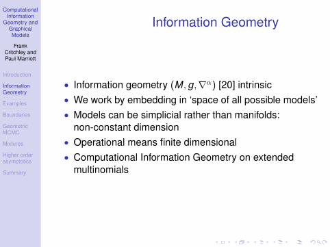
Information Geometry
• Information geometry (M, g,∇α) [20] intrinsic• We work by embedding in ‘space of all possible models’• Models can be simplicial rather than manifolds:
non-constant dimension• Operational means finite dimensional• Computational Information Geometry on extended
multinomials
ComputationalInformation
Geometry andGraphicalModels
FrankCritchley andPaul Marriott
Introduction
InformationGeometry
Examples
Boundaries
GeometricMCMC
Mixtures
Higher orderasymptotics
Summary
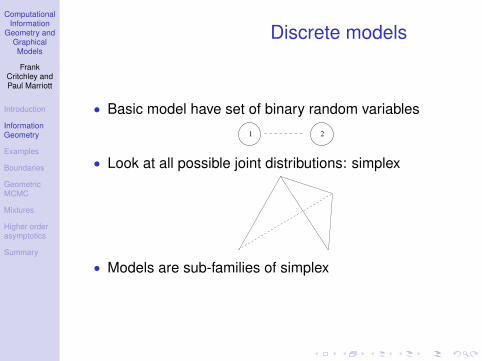
Discrete models
• Basic model have set of binary random variables
1 2
• Look at all possible joint distributions: simplex
• Models are sub-families of simplex

ComputationalInformation
Geometry andGraphicalModels
FrankCritchley andPaul Marriott
Introduction
InformationGeometry
Examples
Boundaries
GeometricMCMC
Mixtures
Higher orderasymptotics
Summary
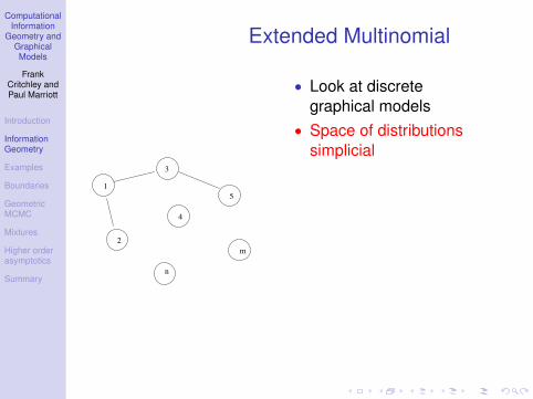
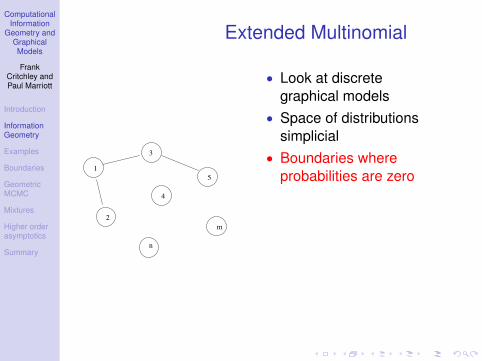
Extended Multinomial
m2
3
4
15
n
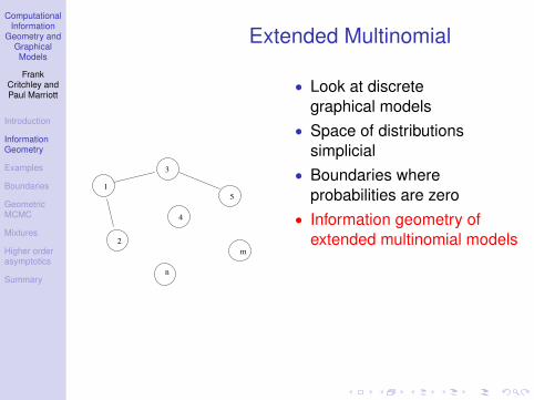
• Look at discretegraphical models
• Space of distributionssimplicial
• Boundaries whereprobabilities are zero
• Information geometry ofextended multinomial models
• applications tographical models andelsewhere
• proxy for space of all models• IG all explicit
ComputationalInformation
Geometry andGraphicalModels
FrankCritchley andPaul Marriott
Introduction
InformationGeometry
Examples
Boundaries
GeometricMCMC
Mixtures
Higher orderasymptotics
Summary
Extended Multinomial
m2
3
4
15
n
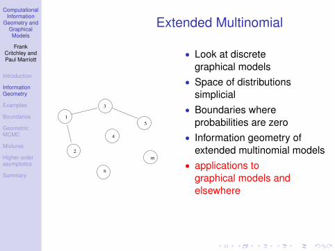
• Look at discretegraphical models
• Space of distributionssimplicial
• Boundaries whereprobabilities are zero
• Information geometry ofextended multinomial models
• applications tographical models andelsewhere
• proxy for space of all models• IG all explicit
ComputationalInformation
Geometry andGraphicalModels
FrankCritchley andPaul Marriott
Introduction
InformationGeometry
Examples
Boundaries
GeometricMCMC
Mixtures
Higher orderasymptotics
Summary
Extended Multinomial
m2
3
4
15
n
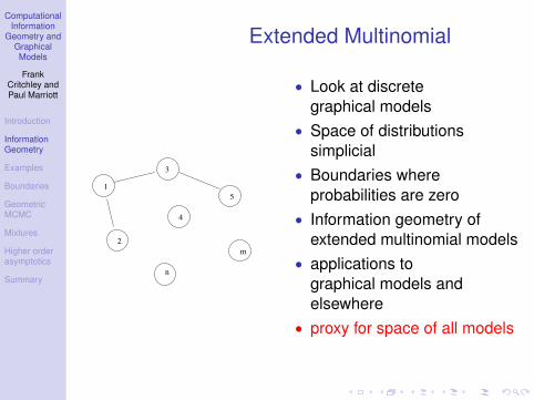
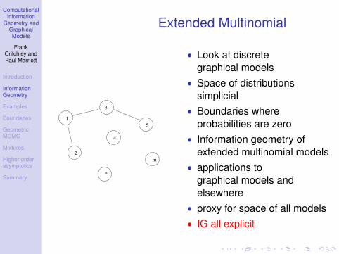
• Look at discretegraphical models
• Space of distributionssimplicial
• Boundaries whereprobabilities are zero
• Information geometry ofextended multinomial models
• applications tographical models andelsewhere
• proxy for space of all models
• IG all explicit
ComputationalInformation
Geometry andGraphicalModels
FrankCritchley andPaul Marriott
Introduction
InformationGeometry
Examples
Boundaries
GeometricMCMC
Mixtures
Higher orderasymptotics
Summary
Extended Multinomial
m2
3
4
15
n
• Look at discretegraphical models
• Space of distributionssimplicial
• Boundaries whereprobabilities are zero
• Information geometry ofextended multinomial models
• applications tographical models andelsewhere
• proxy for space of all models• IG all explicit
ComputationalInformation
Geometry andGraphicalModels
FrankCritchley andPaul Marriott
Introduction
InformationGeometry
Examples
Boundaries
GeometricMCMC
Mixtures
Higher orderasymptotics
Summary
Information Geometry
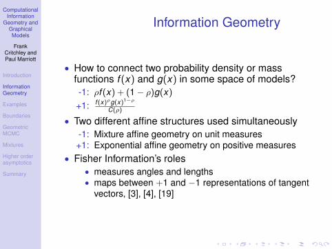
• How to connect two probability density or massfunctions f (x) and g(x) in some space of models?-1: ρf (x) + (1− ρ)g(x)
+1: f (x)ρg(x)1−ρ
C(ρ)
• Two different affine structures used simultaneously-1: Mixture affine geometry on unit measures+1: Exponential affine geometry on positive measures
• Fisher Information’s roles• measures angles and lengths• maps between +1 and −1 representations of tangent
vectors, [3], [4], [19]
ComputationalInformation
Geometry andGraphicalModels
FrankCritchley andPaul Marriott
Introduction
InformationGeometry
Examples
Boundaries
GeometricMCMC
Mixtures
Higher orderasymptotics
Summary
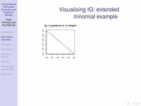
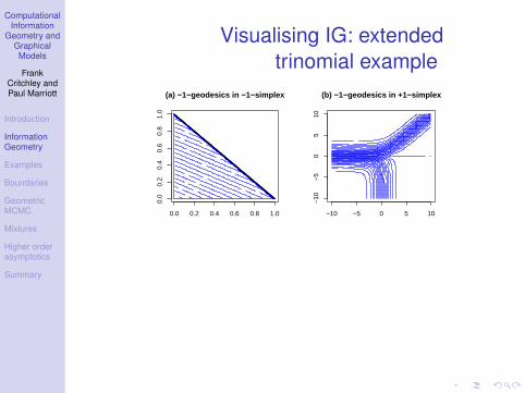
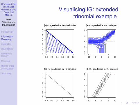
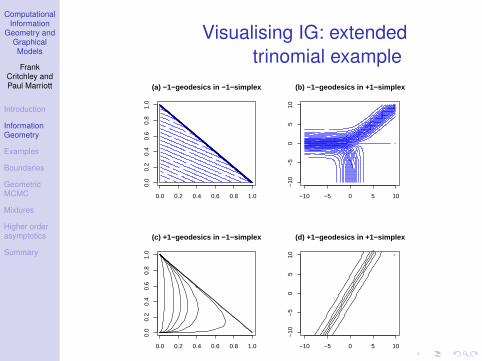
Visualising IG: extendedtrinomial example
(a) −1−geodesics in −1−simplex
0.0 0.2 0.4 0.6 0.8 1.0
0.0
0.2
0.4
0.6
0.8
1.0
(a) −1−geodesics in −1−simplex
0.0 0.2 0.4 0.6 0.8 1.0
0.0
0.2
0.4
0.6
0.8
1.0
(a) −1−geodesics in −1−simplex
0.0 0.2 0.4 0.6 0.8 1.0
0.0
0.2
0.4
0.6
0.8
1.0
(b) −1−geodesics in +1−simplex
−10 −5 0 5 10
−10
−5
05
10
(a) −1−geodesics in −1−simplex
0.0 0.2 0.4 0.6 0.8 1.0
0.0
0.2
0.4
0.6
0.8
1.0
(b) −1−geodesics in +1−simplex
−10 −5 0 5 10
−10
−5
05
10
(c) +1−geodesics in −1−simplex
0.0 0.2 0.4 0.6 0.8 1.0
0.0
0.2
0.4
0.6
0.8
1.0
(d) +1−geodesics in +1−simplex
−10 −5 0 5 10
−10
−5
05
10
(a) −1−geodesics in −1−simplex
0.0 0.2 0.4 0.6 0.8 1.0
0.0
0.2
0.4
0.6
0.8
1.0
(b) −1−geodesics in +1−simplex
−10 −5 0 5 10
−10
−5
05
10
(c) +1−geodesics in −1−simplex
0.0 0.2 0.4 0.6 0.8 1.0
0.0
0.2
0.4
0.6
0.8
1.0
(d) +1−geodesics in +1−simplex
−10 −5 0 5 10
−10
−5
05
10
(a) −1−geodesics in −1−simplex
0.0 0.2 0.4 0.6 0.8 1.0
0.0
0.2
0.4
0.6
0.8
1.0
(b) −1−geodesics in +1−simplex
−10 −5 0 5 10
−10
−5
05
10
(c) +1−geodesics in −1−simplex
0.0 0.2 0.4 0.6 0.8 1.0
0.0
0.2
0.4
0.6
0.8
1.0
(d) +1−geodesics in +1−simplex
−10 −5 0 5 10
−10
−5
05
10

ComputationalInformation
Geometry andGraphicalModels
FrankCritchley andPaul Marriott
Introduction
InformationGeometry
Examples
Boundaries
GeometricMCMC
Mixtures
Higher orderasymptotics
Summary
Visualising IG: extendedtrinomial example
(a) −1−geodesics in −1−simplex
0.0 0.2 0.4 0.6 0.8 1.0
0.0
0.2
0.4
0.6
0.8
1.0
(a) −1−geodesics in −1−simplex
0.0 0.2 0.4 0.6 0.8 1.0
0.0
0.2
0.4
0.6
0.8
1.0
(a) −1−geodesics in −1−simplex
0.0 0.2 0.4 0.6 0.8 1.0
0.0
0.2
0.4
0.6
0.8
1.0
(b) −1−geodesics in +1−simplex
−10 −5 0 5 10
−10
−5
05
10
(a) −1−geodesics in −1−simplex
0.0 0.2 0.4 0.6 0.8 1.0
0.0
0.2
0.4
0.6
0.8
1.0
(b) −1−geodesics in +1−simplex
−10 −5 0 5 10
−10
−5
05
10
(c) +1−geodesics in −1−simplex
0.0 0.2 0.4 0.6 0.8 1.0
0.0
0.2
0.4
0.6
0.8
1.0
(d) +1−geodesics in +1−simplex
−10 −5 0 5 10
−10
−5
05
10
(a) −1−geodesics in −1−simplex
0.0 0.2 0.4 0.6 0.8 1.0
0.0
0.2
0.4
0.6
0.8
1.0
(b) −1−geodesics in +1−simplex
−10 −5 0 5 10
−10
−5
05
10
(c) +1−geodesics in −1−simplex
0.0 0.2 0.4 0.6 0.8 1.0
0.0
0.2
0.4
0.6
0.8
1.0
(d) +1−geodesics in +1−simplex
−10 −5 0 5 10
−10
−5
05
10
(a) −1−geodesics in −1−simplex
0.0 0.2 0.4 0.6 0.8 1.0
0.0
0.2
0.4
0.6
0.8
1.0
(b) −1−geodesics in +1−simplex
−10 −5 0 5 10
−10
−5
05
10
(c) +1−geodesics in −1−simplex
0.0 0.2 0.4 0.6 0.8 1.0
0.0
0.2
0.4
0.6
0.8
1.0
(d) +1−geodesics in +1−simplex
−10 −5 0 5 10
−10
−5
05
10
ComputationalInformation
Geometry andGraphicalModels
FrankCritchley andPaul Marriott
Introduction
InformationGeometry
Examples
Boundaries
GeometricMCMC
Mixtures
Higher orderasymptotics
Summary
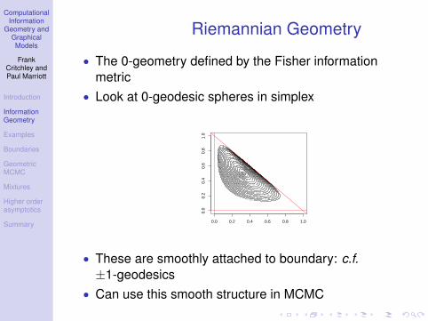
Riemannian Geometry
• The 0-geometry defined by the Fisher informationmetric
• Look at 0-geodesic spheres in simplex
0.0 0.2 0.4 0.6 0.8 1.0
0.0
0.2
0.4
0.6
0.8
1.0
• These are smoothly attached to boundary: c.f.±1-geodesics
• Can use this smooth structure in MCMC
ComputationalInformation
Geometry andGraphicalModels
FrankCritchley andPaul Marriott
Introduction
InformationGeometry
Examples
Boundaries
GeometricMCMC
Mixtures
Higher orderasymptotics
Summary
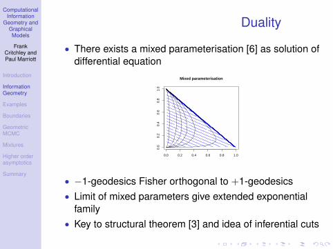
Duality
• There exists a mixed parameterisation [6] as solution ofdifferential equation
Mixed parameterisation
0.0 0.2 0.4 0.6 0.8 1.00.
00.
20.
40.
60.
81.
0
• −1-geodesics Fisher orthogonal to +1-geodesics• Limit of mixed parameters give extended exponential
family• Key to structural theorem [3] and idea of inferential cuts
ComputationalInformation
Geometry andGraphicalModels
FrankCritchley andPaul Marriott
Introduction
InformationGeometry
Examples
Boundaries
GeometricMCMC
Mixtures
Higher orderasymptotics
Summary
Geometry of likelihood
For sparse extended multinomial models:• Quadratic approximations to log-likelihood fail globally• Many −1-flat directions• MCMC• Asymptotics
ComputationalInformation
Geometry andGraphicalModels
FrankCritchley andPaul Marriott
Introduction
InformationGeometry
Examples
Boundaries
GeometricMCMC
Mixtures
Higher orderasymptotics
Summary
Examples: Graphs, Networksand IG
• Full exponential families [17]• Very high-dimensional models [21] - MCMC is one tool
here• Curved exponential families - curvature can be very
high• Closure of exponential families- boundaries
ComputationalInformation
Geometry andGraphicalModels
FrankCritchley andPaul Marriott
Introduction
InformationGeometry
Examples
Boundaries
GeometricMCMC
Mixtures
Higher orderasymptotics
Summary
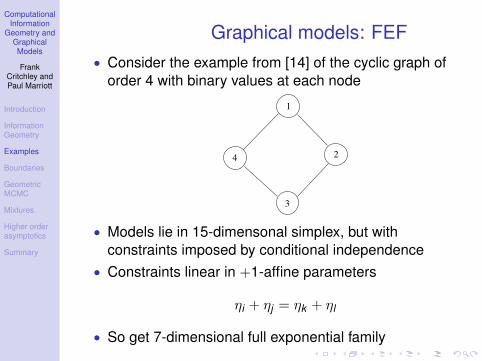
Graphical models: FEF• Consider the example from [14] of the cyclic graph of
order 4 with binary values at each node
1
2
3
4
• Models lie in 15-dimensonal simplex, but withconstraints imposed by conditional independence
• Constraints linear in +1-affine parameters
ηi + ηj = ηk + ηl
• So get 7-dimensional full exponential family
ComputationalInformation
Geometry andGraphicalModels
FrankCritchley andPaul Marriott
Introduction
InformationGeometry
Examples
Boundaries
GeometricMCMC
Mixtures
Higher orderasymptotics
Summary
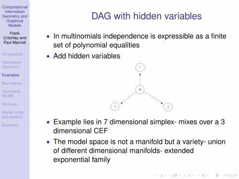
DAG with hidden variables
• In multinomials independence is expressible as a finiteset of polynomial equalities
• Add hidden variables
2
1
H
3
• Example lies in 7 dimensional simplex- mixes over a 3dimensional CEF
• The model space is not a manifold but a variety- unionof different dimensional manifolds- extendedexponential family
ComputationalInformation
Geometry andGraphicalModels
FrankCritchley andPaul Marriott
Introduction
InformationGeometry
Examples
Boundaries
GeometricMCMC
Mixtures
Higher orderasymptotics
Summary
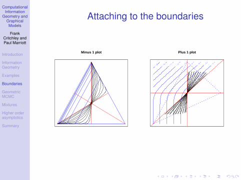
Attaching to the boundaries
• Models are low-dimensional families within highdimensional simplexes
• Need to understand how models are attached toboundaries
• Extended exponential families: see also [30], [9]• Need to be able to compute limit points in
computationally efficient way• Use linear programming and convex geometry
techniques• The following plot is generic
ComputationalInformation
Geometry andGraphicalModels
FrankCritchley andPaul Marriott
Introduction
InformationGeometry
Examples
Boundaries
GeometricMCMC
Mixtures
Higher orderasymptotics
Summary
Attaching to the boundaries
Minus 1 plot
●
Plus 1 plot
ComputationalInformation
Geometry andGraphicalModels
FrankCritchley andPaul Marriott
Introduction
InformationGeometry
Examples
Boundaries
GeometricMCMC
Mixtures
Higher orderasymptotics
Summary
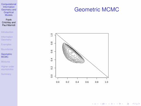
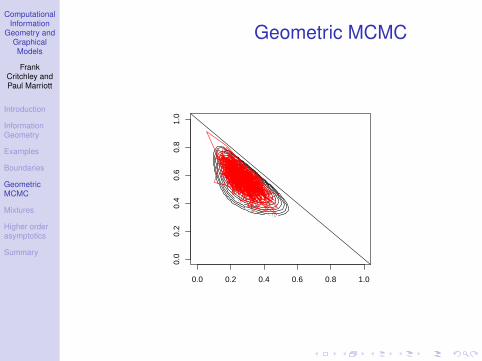
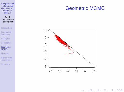
Geometric MCMC
• When doing MCMC on models the boundaries matter• Riemann manifold Metropolis adjusted Langevin
algorithm, [13] uses Fisher metric structure.• Use a Metropolis-Hastings where the random-walk
proposals have variance determined by Fisher metric• Have seen how the 0-geometry smoothly attaches the
boundaries• Other geometric approaches are under active
development - cuts and mixed parameterisations
ComputationalInformation
Geometry andGraphicalModels
FrankCritchley andPaul Marriott
Introduction
InformationGeometry
Examples
Boundaries
GeometricMCMC
Mixtures
Higher orderasymptotics
Summary
Geometric MCMC
0.0 0.2 0.4 0.6 0.8 1.0
0.0
0.2
0.4
0.6
0.8
1.0
ComputationalInformation
Geometry andGraphicalModels
FrankCritchley andPaul Marriott
Introduction
InformationGeometry
Examples
Boundaries
GeometricMCMC
Mixtures
Higher orderasymptotics
Summary
Geometric MCMC
0.0 0.2 0.4 0.6 0.8 1.0
0.0
0.2
0.4
0.6
0.8
1.0

ComputationalInformation
Geometry andGraphicalModels
FrankCritchley andPaul Marriott
Introduction
InformationGeometry
Examples
Boundaries
GeometricMCMC
Mixtures
Higher orderasymptotics
Summary
Geometric MCMC
0.0 0.2 0.4 0.6 0.8 1.0
0.0
0.2
0.4
0.6
0.8
1.0
ComputationalInformation
Geometry andGraphicalModels
FrankCritchley andPaul Marriott
Introduction
InformationGeometry
Examples
Boundaries
GeometricMCMC
Mixtures
Higher orderasymptotics
Summary
Geometric MCMC
0.0 0.2 0.4 0.6 0.8 1.0
0.0
0.2
0.4
0.6
0.8
1.0
ComputationalInformation
Geometry andGraphicalModels
FrankCritchley andPaul Marriott
Introduction
InformationGeometry
Examples
Boundaries
GeometricMCMC
Mixtures
Higher orderasymptotics
Summary
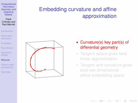
Embedding curvature and affineapproximation
• Curvature(s) key part(s) ofdifferential geometry
• Tangent space gives bestlinear approximation
• Tangent and curvature givesbest two dimensionalaffine embedding space
ComputationalInformation
Geometry andGraphicalModels
FrankCritchley andPaul Marriott
Introduction
InformationGeometry
Examples
Boundaries
GeometricMCMC
Mixtures
Higher orderasymptotics
Summary
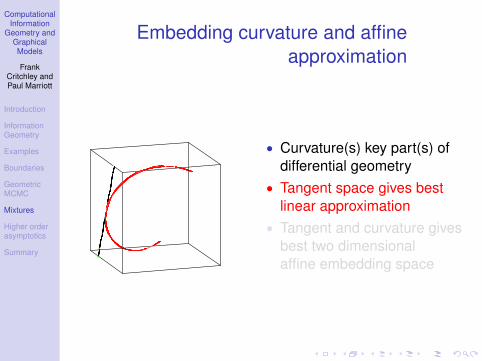
Embedding curvature and affineapproximation
• Curvature(s) key part(s) ofdifferential geometry
• Tangent space gives bestlinear approximation
• Tangent and curvature givesbest two dimensionalaffine embedding space
ComputationalInformation
Geometry andGraphicalModels
FrankCritchley andPaul Marriott
Introduction
InformationGeometry
Examples
Boundaries
GeometricMCMC
Mixtures
Higher orderasymptotics
Summary
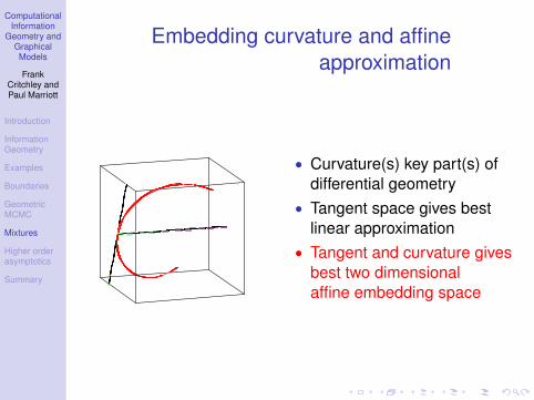
Embedding curvature and affineapproximation
• Curvature(s) key part(s) ofdifferential geometry
• Tangent space gives bestlinear approximation
• Tangent and curvature givesbest two dimensionalaffine embedding space
ComputationalInformation
Geometry andGraphicalModels
FrankCritchley andPaul Marriott
Introduction
InformationGeometry
Examples
Boundaries
GeometricMCMC
Mixtures
Higher orderasymptotics
Summary
Curvature and DimensionReduction
• Dimension reduction (best approximating subspaces)via tangent and curvature
• Different affine geometries give different dimensionreduction
• Low dimensional +1-affine spaces give approximatesufficient statistics [28]
• Low dimensional −1 approximations give limits toidentification and computation in mixture models [27],[2]
ComputationalInformation
Geometry andGraphicalModels
FrankCritchley andPaul Marriott
Introduction
InformationGeometry
Examples
Boundaries
GeometricMCMC
Mixtures
Higher orderasymptotics
Summary
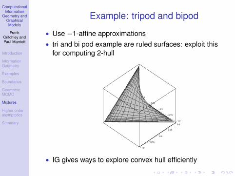
Example: tripod and bipod
• Use −1-affine approximations• tri and bi pod example are ruled surfaces: exploit this
for computing 2-hull
0.0
0.25
0.5
0.75
1.00.0
0.25
0.5
0.75
1.0
• IG gives ways to explore convex hull efficiently
ComputationalInformation
Geometry andGraphicalModels
FrankCritchley andPaul Marriott
Introduction
InformationGeometry
Examples
Boundaries
GeometricMCMC
Mixtures
Higher orderasymptotics
Summary
Mixing paradox
• There is a paradoxical aspect to mixing in highdimensional extended multinomial model
• The convex hull of any open interval of aone-dimensional exponential family is of full dimension· · ·
• This is due to total positivity• · · · But, there exist low dimensional approximations to
this convex hull based on curvature, [2]
ComputationalInformation
Geometry andGraphicalModels
FrankCritchley andPaul Marriott
Introduction
InformationGeometry
Examples
Boundaries
GeometricMCMC
Mixtures
Higher orderasymptotics
Summary
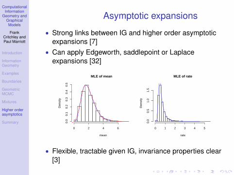
Asymptotic expansions
• Strong links between IG and higher order asymptoticexpansions [7]
• Can apply Edgeworth, saddlepoint or Laplaceexpansions [32]
MLE of mean
mean
Den
sity
0 2 4 6
0.0
0.1
0.2
0.3
0.4
0.5
MLE of rate
rate
Den
sity
0 1 2 3 4 5
0.0
0.5
1.0
1.5
• Flexible, tractable given IG, invariance properties clear[3]
ComputationalInformation
Geometry andGraphicalModels
FrankCritchley andPaul Marriott
Introduction
InformationGeometry
Examples
Boundaries
GeometricMCMC
Mixtures
Higher orderasymptotics
Summary
Asymptotic expansions
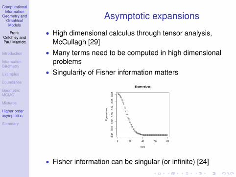
• High dimensional calculus through tensor analysis,McCullagh [29]
• Many terms need to be computed in high dimensionalproblems
• Singularity of Fisher information matters
0 20 40 60 80
0.00
0.01
0.02
0.03
0.04
0.05
0.06
Eigenvalues
rank
Eigenvalues
• Fisher information can be singular (or infinite) [24]
ComputationalInformation
Geometry andGraphicalModels
FrankCritchley andPaul Marriott
Introduction
InformationGeometry
Examples
Boundaries
GeometricMCMC
Mixtures
Higher orderasymptotics
Summary
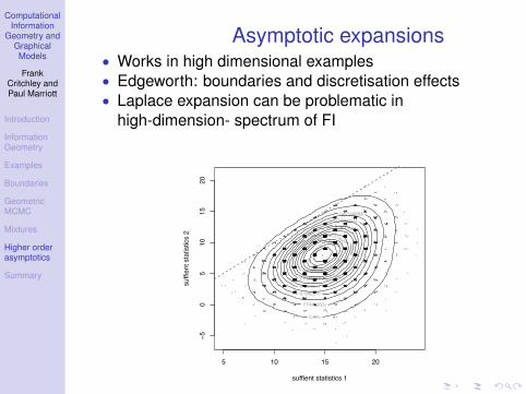
Asymptotic expansions• Works in high dimensional examples• Edgeworth: boundaries and discretisation effects• Laplace expansion can be problematic in
high-dimension- spectrum of FI
5 10 15 20
!50
510
1520
suffient statistics 1
suffi
ent s
tatis
tics
2
ComputationalInformation
Geometry andGraphicalModels
FrankCritchley andPaul Marriott
Introduction
InformationGeometry
Examples
Boundaries
GeometricMCMC
Mixtures
Higher orderasymptotics
Summary
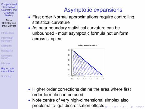
Asymptotic expansions• First order Normal approximations require controlling
statistical curvature• As near boundary statistical curvature can be
unbounded - most asymptotic formula not uniformacross simplex
Mixed parameterisation
0.0 0.2 0.4 0.6 0.8 1.0
0.0
0.2
0.4
0.6
0.8
1.0
• Higher order corrections define the area where firstorder formula can be used
• Note centre of very high-dimensional simplex alsoproblematic- get discretisation effects
ComputationalInformation
Geometry andGraphicalModels
FrankCritchley andPaul Marriott
Introduction
InformationGeometry
Examples
Boundaries
GeometricMCMC
Mixtures
Higher orderasymptotics
Summary
Summary
• Information Geometry - our embedding approach• Focus on computation (CIG)• Boundaries - essential for graphical models• MCMC - geometric approach• Curvature and mixture models• Simplicial asymptotics - lack of uniformity• CIG useful generally in statistical modelling
ComputationalInformation
Geometry andGraphicalModels
FrankCritchley andPaul Marriott
Introduction
InformationGeometry
Examples
Boundaries
GeometricMCMC
Mixtures
Higher orderasymptotics
Summary
References I[1] Anaya-Izquierdo, K., Critchley, F, Marriott P. & Vos P. (2010),
Towards information geometry on the space of all distributions,Preprint
[2] Anaya-Izquierdo, K and Marriott, P. (2007) Local mixtures ofExponential families, Bernoulli Vol. 13, No. 3, 623-640.
[3] Amari, S.-I. (1985). Differential-Geometrical Methods in Statistics.Lecture Notes in Statistics, No. 28, New York: Springer.
[4] Amari, S.-I. and Nagaoka, H. (2000). Methods of InformationGeometry. Providence, Rhode Island: American MathematicalSociety.
[5] Barndorff-Nielsen, O., (1978) Information and exponential families instatistical theory, London: John Wiley & Sons
[6] Barndorff-Nielsen, O. E. and Blaesild, P. (1983). Exponential modelswith affine dual foliations. Annals of Statistics, 11(3):753–769.
[7] Barndorff-Nielsen, O.E. and Cox, D.R, (1994), Inference andAsymptotics, Chapman & Hall:London
ComputationalInformation
Geometry andGraphicalModels
FrankCritchley andPaul Marriott
Introduction
InformationGeometry
Examples
Boundaries
GeometricMCMC
Mixtures
Higher orderasymptotics
Summary
References II
[8] Brown, L. D. (1986). Fundamentals of statistical exponentialfamilies: with applications in statistical decision theory, Institute ofMathematical Statistics
[9] Csiszar, I. and Matus, F., (2005). Closures of exponential families,The Annals of Probability, 33(2):582–600
[10] Efron, B. (1975). Defining the curvature of a statistical problem (withapplications to second order efficiency), The Annals of Statistics,3(6):1189–1242
[11] Fukumizu, K. (2005). Infinite dimensional exponential families byreproducing kernel hilbert spaces. Proceedings of the 2ndInternational Symposium on Information Geometry and itsApplications,p324-333.
[12] Gibilisco, P. and Pistone, G. (1998). Connections on non-parametricstatistical manifolds by orlicz space geometry. Infinite DimensionalAnalysis, Quantum Probability and Related Topics, 1(2):325-347.
ComputationalInformation
Geometry andGraphicalModels
FrankCritchley andPaul Marriott
Introduction
InformationGeometry
Examples
Boundaries
GeometricMCMC
Mixtures
Higher orderasymptotics
Summary
References III
[13] Girolami M. and Calderhead, B. (2011), Riemann manifold Langevinand Hamiltonian Monte Carlo methods, J. R. Statist. Soc. B 73, Part2, pp. 1-37
[14] D. Geiger, D.Heckerman, H.King and C. Meek (2001) StratifiedExponential Families: Graphical Models and Model Selection,Annals of Statistics, Vol. 29, No. 2, pp 505-529
[15] Grunwald P.D. and Dawid A.P. (2004) Game theory, maximumentropy, minimum discrepancy and robust Bayesian decision theory,Annals of Statistics, 32, 4 1267-1433
[16] Hand, D.J., Daly, F., Lunn, A.D., McConway, K.J. and Ostrowski, E.(1994), A handbook of small data sets , Chapman & Hall, London.
[17] D. Hunter, (2007) Curved exponential family models for socialnetworks, Social Networks, 29 216–230.
[18] Hunter D, Handcock M. (2006) Inference in curved exponentialfamily models for networks J. of Computational and GraphicalStatistics 15, 565-583
ComputationalInformation
Geometry andGraphicalModels
FrankCritchley andPaul Marriott
Introduction
InformationGeometry
Examples
Boundaries
GeometricMCMC
Mixtures
Higher orderasymptotics
Summary
References IV
[19] Kass, R. E. and Vos, P. W. (1997). Geometrical Foundations ofAsymptotic Inference. New York: Wiley.
[20] Lauritzen, S. L. (1987). Statistical manifolds, in Differential geometryin statistical inference: IMS
[21] Lazega, E., Pattison, P.E., (1999) Multiplexity, generalized exchangeand cooperation in organizations: a case study. Social Networks 21,67–90
[22] L. L. Kupper L.L., and Haseman J.K., (1978), The Use of aCorrelated Binomial Model for the Analysis of Certain ToxicologicalExperiments, Biometrics, Vol. 34, No. 1 (Mar., 1978), pp. 69-76
[23] Mary L. Lesperance and John D. Kalbfleisch (1992) An Algorithmfor Computing the Nonparametric MLE of a Mixing DistributionJASAVol. 87, No. 417 (Mar., 1992), pp. 120-126
[24] Li P., Chen J., & Marriott P., (2009) Non-finite Fisher information andhomogeneity: the EM approach, Biometrika 96, 2 pp 411-426.
ComputationalInformation
Geometry andGraphicalModels
FrankCritchley andPaul Marriott
Introduction
InformationGeometry
Examples
Boundaries
GeometricMCMC
Mixtures
Higher orderasymptotics
Summary
References V
[25] Lindsay, B.G. (1995). Mixture models: Theory, Geometry, andApplications, Hayward CA: Institute of Mathematical Sciences.
[26] Marriott P and West S, (2002), On the Geometry of CensoredModels, Calcutta Statistical Association Bulletin 52, pp 235-250.
[27] Marriott, P (2002), On the local geometry of Mixture Models,Biometrika, 89, 1, pp 77-89
[28] Marriott, P., & Vos, P. (2004), On The Global Geometry ofParametric Models and Information Recovery, Bernoulli, 10 (2), 1-11
[29] McCullagh P. (1987) Tensor Methods in Statistics, Chapman andHall, London.
[30] Rinaldo, Alessandro and Fienberg Stephen (2009), On thegeometry of discrete exponential families with applications toexponential random graph models, EJS, 3, pp. 446-484
[31] Snijders, T. A. B. (2002), Markov Chain Monte Carlo Estimation ofExponential Random Graph Models, Journal of Social Structure, 3.
ComputationalInformation
Geometry andGraphicalModels
FrankCritchley andPaul Marriott
Introduction
InformationGeometry
Examples
Boundaries
GeometricMCMC
Mixtures
Higher orderasymptotics
Summary
References VI
[32] Small, C.G. (2010) Expansions and asymptotics for statistics,Chapman and Hall
[33] Strauss, D., and Ikeda, M. (1990), Pseudolikelihood Estimation forSocial Networks,Journal of the American Statistical Association ,85, 204–212.
[34] Shun Z and McCullagh P. (1995) Laplace approximations of highdimensional integrals JRSS B