UltraScienceNet Research Testbed Enabling Computational Genomics Project Overview
date post
19-Dec-2015Category
view
217download
2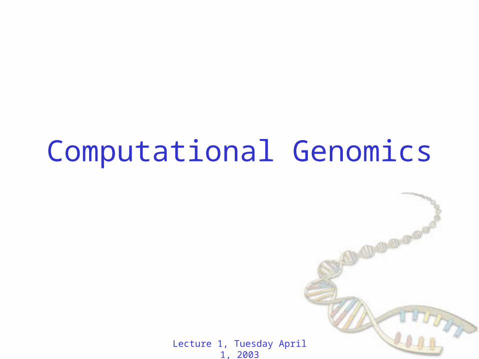
Computational Genomics
Lecture 1, Tuesday April 1, 2003
Lecture 1, Tuesday April 1, 2003
Biology in One Slide
Lecture 1, Tuesday April 1, 2003
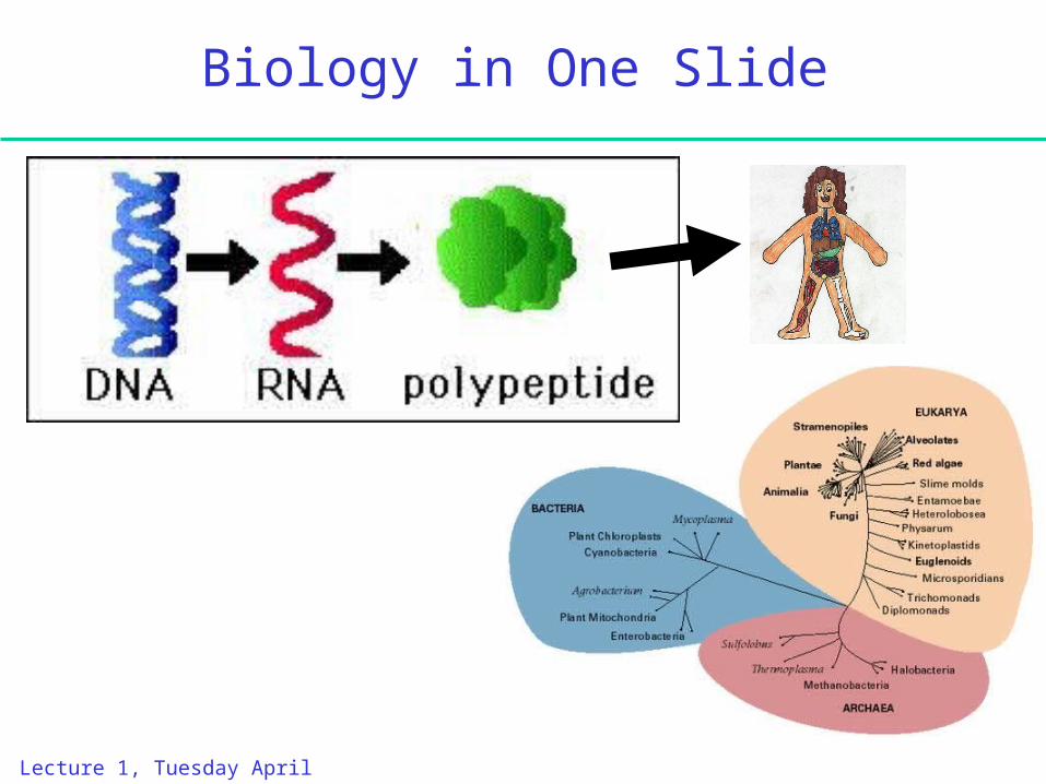
High Throughput Biology
1. DNA Sequencing
…ACGTGACTGAGGACCGTGCGACTGAGACTGACTGGGTCTAGCTAGACTACGTTTTATATATATATACGTCGTCGTACTGATGACTAGATTACAGACTGATTTAGATACCTGACTGATTTTAAAAAAATATT…
Lecture 1, Tuesday April 1, 2003
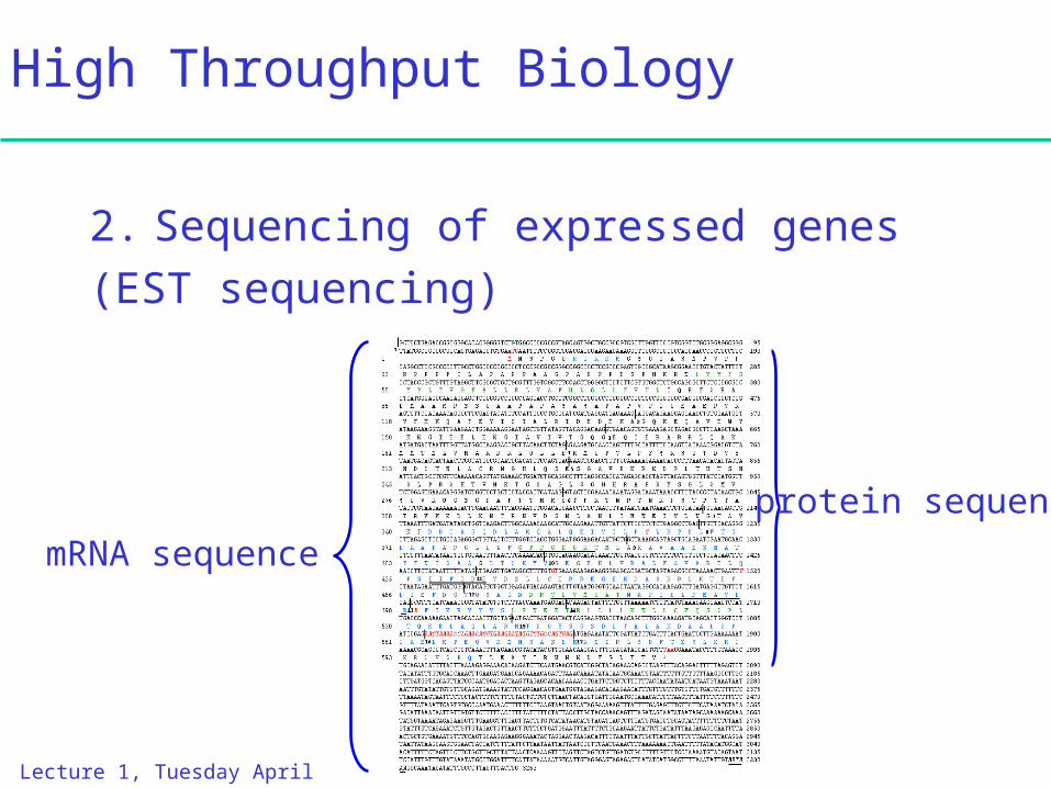
High Throughput Biology
2. Sequencing of expressed genes(EST sequencing)
mRNA sequence
protein sequence
Lecture 1, Tuesday April 1, 2003
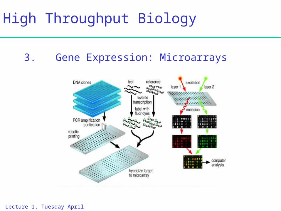
High Throughput Biology
3. Gene Expression: Microarrays
Lecture 1, Tuesday April 1, 2003
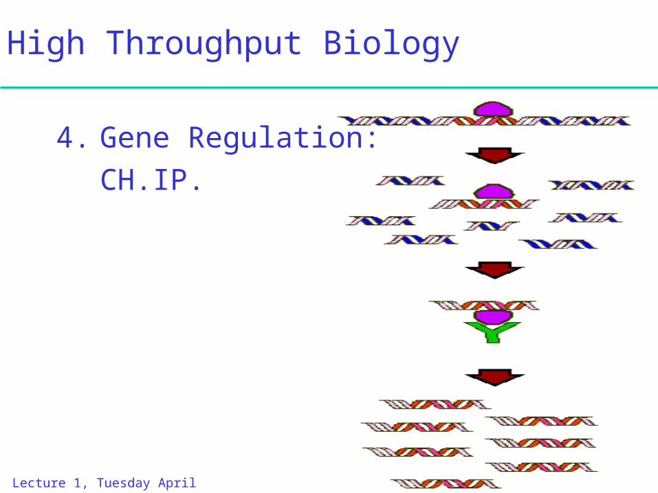
High Throughput Biology
4. Gene Regulation: CH.IP.
Lecture 1, Tuesday April 1, 2003
The goals of genomics
• Study organisms at the DNA level
– Identify “parts” (genes, etc)– Figure out “connections” between
“parts”
• Study evolution at the DNA level
– Compare organisms– Uncover evolutionary history
Lecture 1, Tuesday April 1, 2003
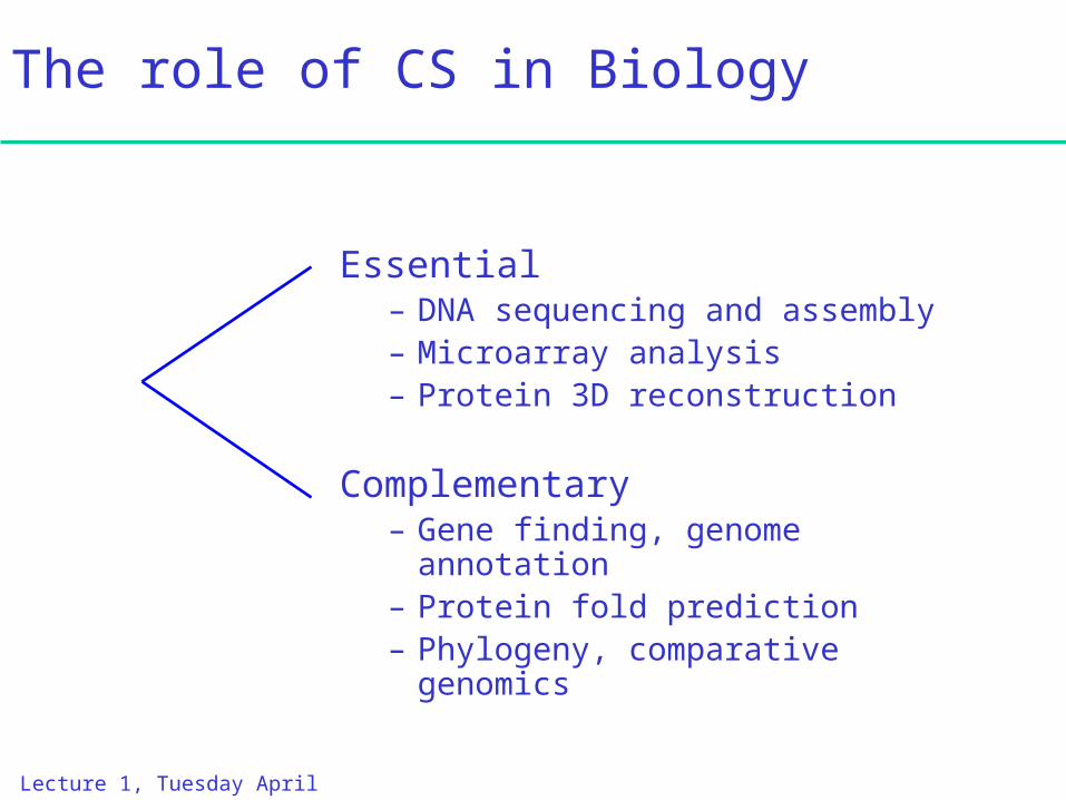
The role of CS in Biology
Essential– DNA sequencing and assembly– Microarray analysis– Protein 3D reconstruction
Complementary– Gene finding, genome annotation– Protein fold prediction– Phylogeny, comparative
genomics
Lecture 1, Tuesday April 1, 2003
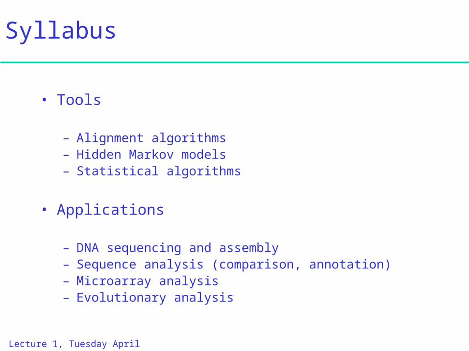
Syllabus
• Tools
– Alignment algorithms– Hidden Markov models– Statistical algorithms
• Applications
– DNA sequencing and assembly– Sequence analysis (comparison, annotation)– Microarray analysis– Evolutionary analysis
Lecture 1, Tuesday April 1, 2003
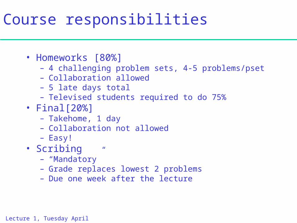
Course responsibilities
• Homeworks [80%]– 4 challenging problem sets, 4-5 problems/pset– Collaboration allowed– 5 late days total– Televised students required to do 75%
• Final [20%]– Takehome, 1 day– Collaboration not allowed– Easy!
• Scribing– “Mandatory”– Grade replaces lowest 2 problems– Due one week after the lecture
Lecture 1, Tuesday April 1, 2003
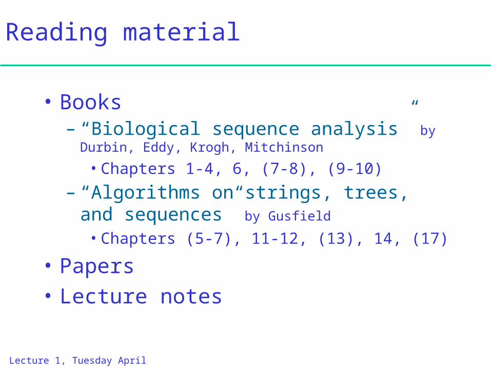
Reading material
• Books– “Biological sequence analysis” by
Durbin, Eddy, Krogh, Mitchinson
• Chapters 1-4, 6, (7-8), (9-10)
– “Algorithms on strings, trees, and sequences” by Gusfield
• Chapters (5-7), 11-12, (13), 14, (17)
• Papers• Lecture notes
Topic 1. Sequence Alignment
Lecture 1, Tuesday April 1, 2003
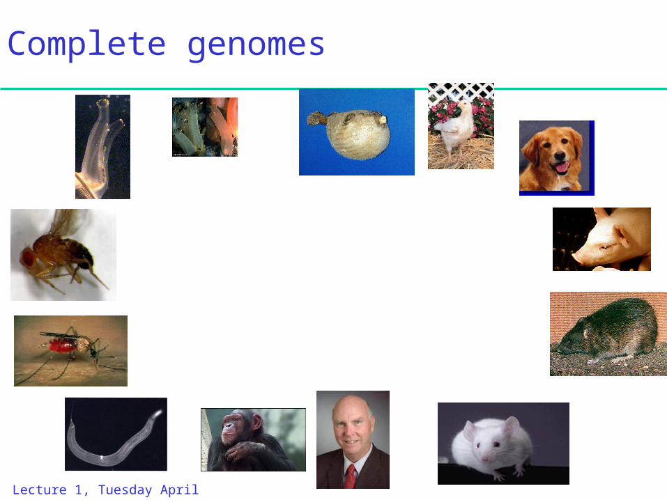
Complete genomes
Lecture 1, Tuesday April 1, 2003
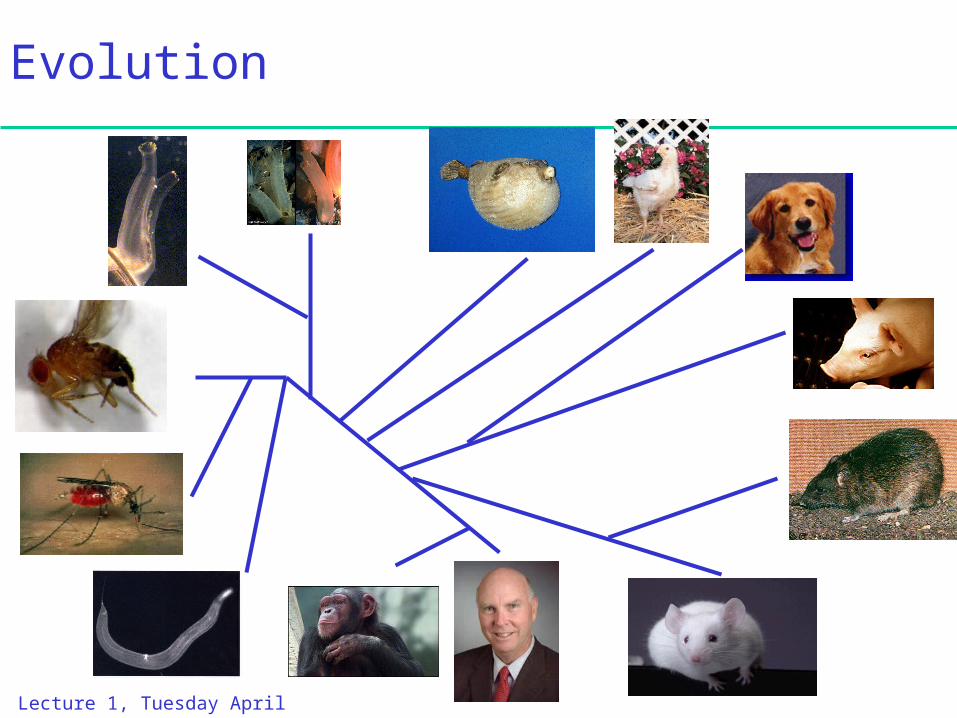
Evolution
Lecture 1, Tuesday April 1, 2003
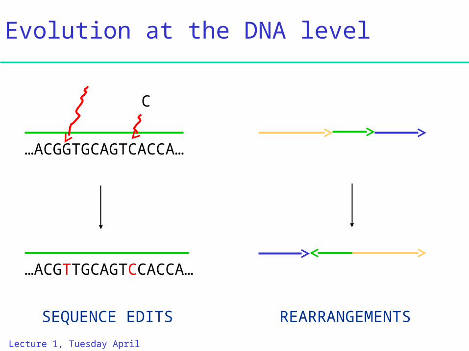
Evolution at the DNA level
…ACGGTGCAGTCACCA…
…ACGTTGCAGTCCACCA…
C
SEQUENCE EDITS REARRANGEMENTS
Lecture 1, Tuesday April 1, 2003
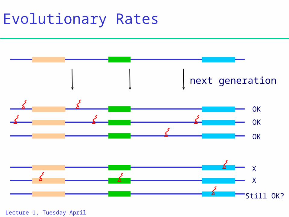
Evolutionary Rates
OK
OK
OK
X
X
Still OK?
next generation
Lecture 1, Tuesday April 1, 2003
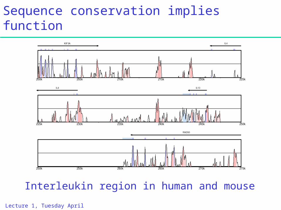
Sequence conservation implies function
Interleukin region in human and mouse
Lecture 1, Tuesday April 1, 2003
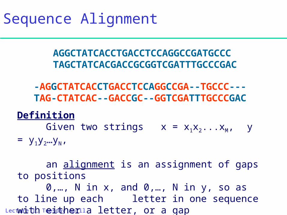
Sequence Alignment
-AGGCTATCACCTGACCTCCAGGCCGA--TGCCC---TAG-CTATCAC--GACCGC--GGTCGATTTGCCCGAC
DefinitionGiven two strings x = x1x2...xM, y
= y1y2…yN,
an alignment is an assignment of gaps to positions
0,…, N in x, and 0,…, N in y, so as to line up each letter in one sequence with either a letter, or a gap
in the other sequence
AGGCTATCACCTGACCTCCAGGCCGATGCCCTAGCTATCACGACCGCGGTCGATTTGCCCGAC
Lecture 1, Tuesday April 1, 2003
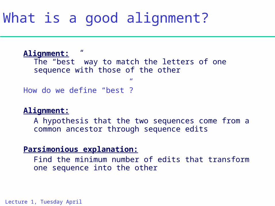
What is a good alignment?
Alignment: The “best” way to match the letters of one sequence with those of the other
How do we define “best”?
Alignment:A hypothesis that the two sequences come from a common ancestor through sequence edits
Parsimonious explanation:Find the minimum number of edits that transform one sequence into the other
Lecture 1, Tuesday April 1, 2003
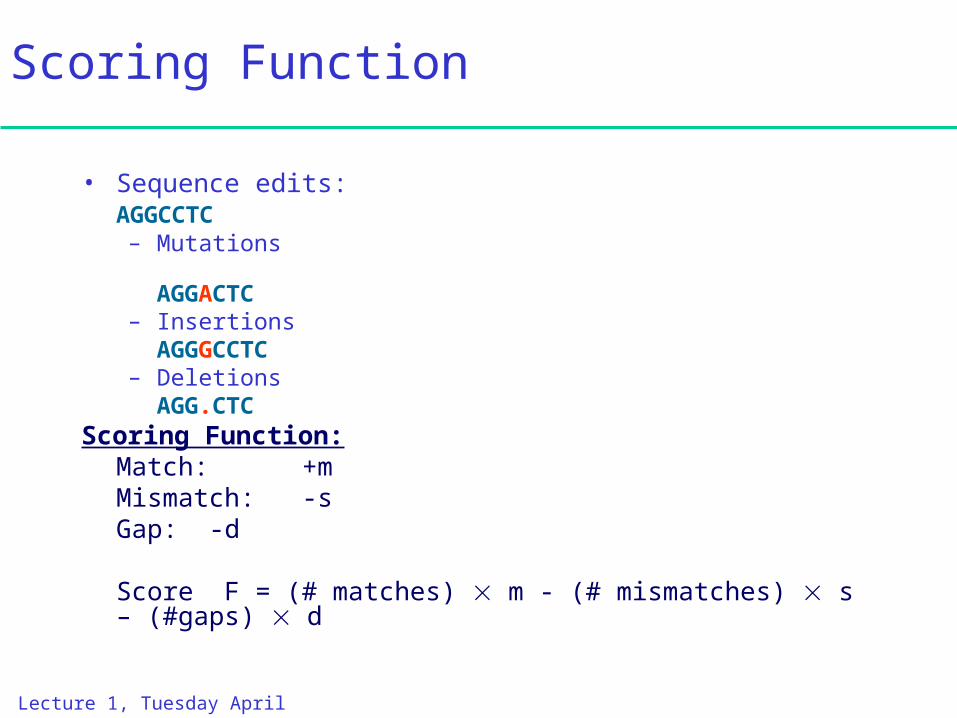
Scoring Function
• Sequence edits:AGGCCTC
– Mutations AGGACTC
– InsertionsAGGGCCTC
– DeletionsAGG.CTC
Scoring Function:Match: +mMismatch: -sGap: -d
Score F = (# matches) m - (# mismatches) s – (#gaps) d
Lecture 1, Tuesday April 1, 2003
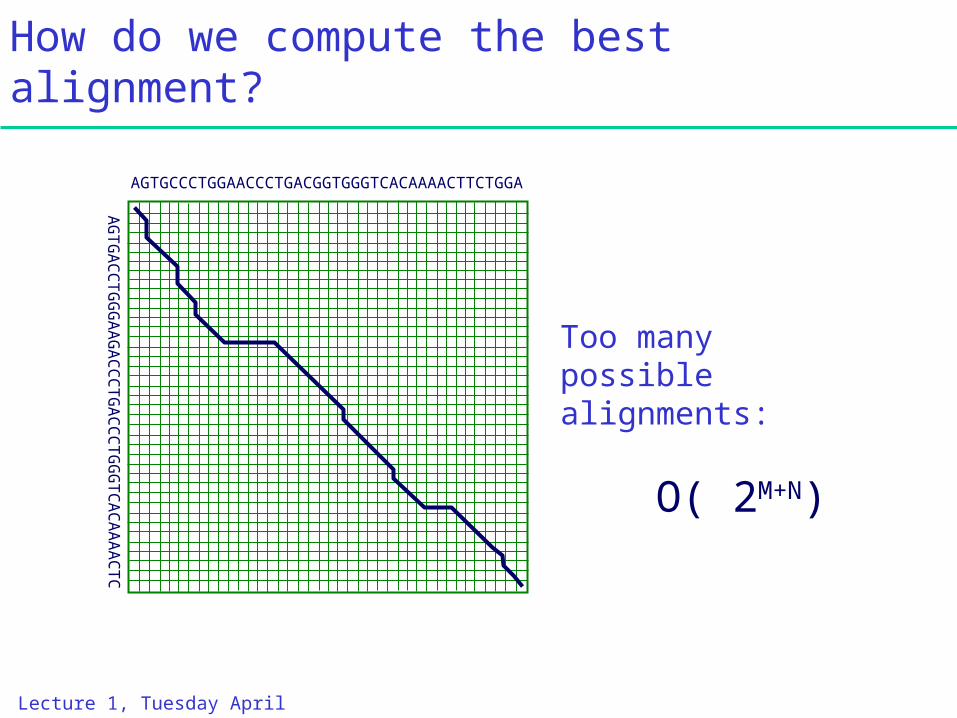
How do we compute the best alignment?
AGTGCCCTGGAACCCTGACGGTGGGTCACAAAACTTCTGGA
AGTGACCTGGGAAGACCCTGACCCTGGGTCACAAAACTC
Too many possible alignments:
O( 2M+N)
Lecture 1, Tuesday April 1, 2003
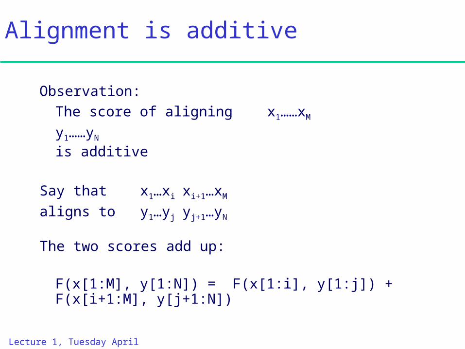
Alignment is additive
Observation:The score of aligning x1……xM
y1……yN
is additive
Say that x1…xi xi+1…xM
aligns to y1…yj yj+1…yN
The two scores add up:
F(x[1:M], y[1:N]) = F(x[1:i], y[1:j]) + F(x[i+1:M], y[j+1:N])
Lecture 1, Tuesday April 1, 2003
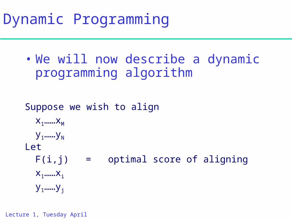
Dynamic Programming
• We will now describe a dynamic programming algorithm
Suppose we wish to alignx1……xM
y1……yN
Let F(i,j) = optimal score of aligning
x1……xi
y1……yj
Lecture 1, Tuesday April 1, 2003
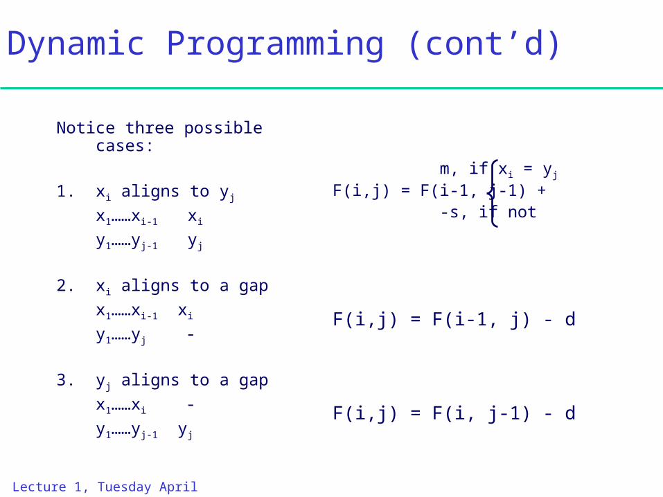
Dynamic Programming (cont’d)
Notice three possible cases:
1. xi aligns to yj
x1……xi-1 xi
y1……yj-1 yj
2. xi aligns to a gap
x1……xi-1 xi
y1……yj -
3. yj aligns to a gap
x1……xi -
y1……yj-1 yj
m, if xi = yj
F(i,j) = F(i-1, j-1) + -s, if not
F(i,j) = F(i-1, j) - d
F(i,j) = F(i, j-1) - d
Lecture 1, Tuesday April 1, 2003
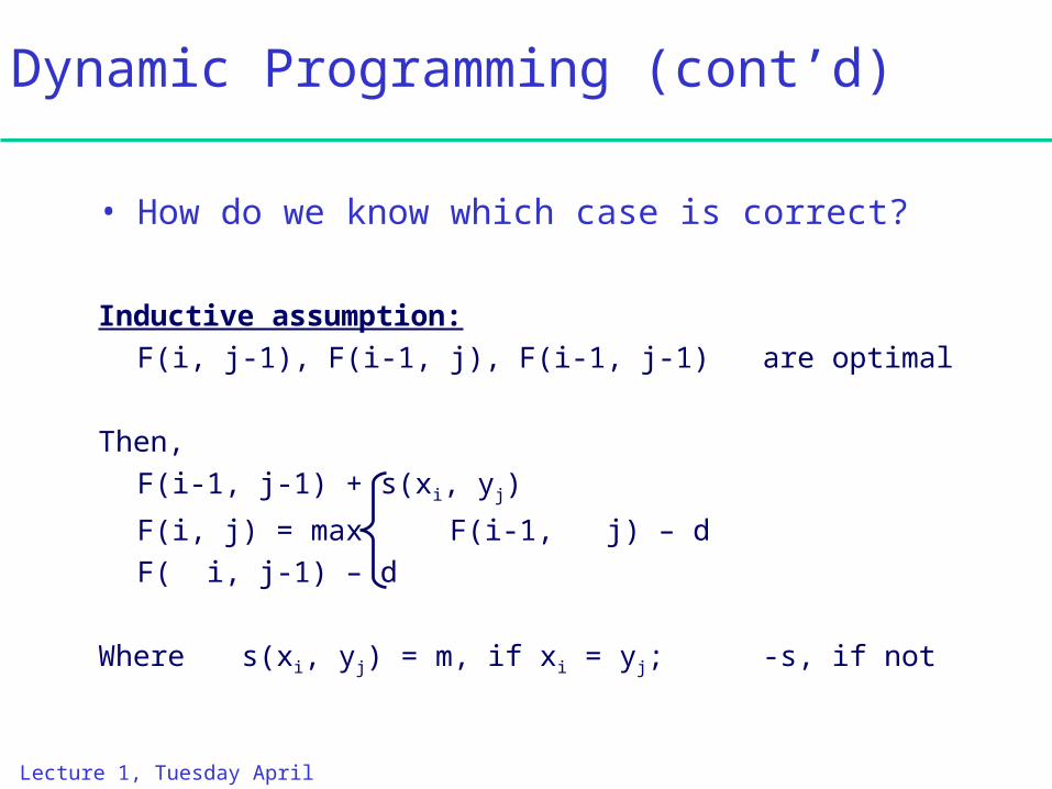
Dynamic Programming (cont’d)
• How do we know which case is correct?
Inductive assumption:F(i, j-1), F(i-1, j), F(i-1, j-1) are optimal
Then,F(i-1, j-1) + s(xi, yj)
F(i, j) = max F(i-1, j) – dF( i, j-1) – d
Where s(xi, yj) = m, if xi = yj; -s, if not
Lecture 1, Tuesday April 1, 2003
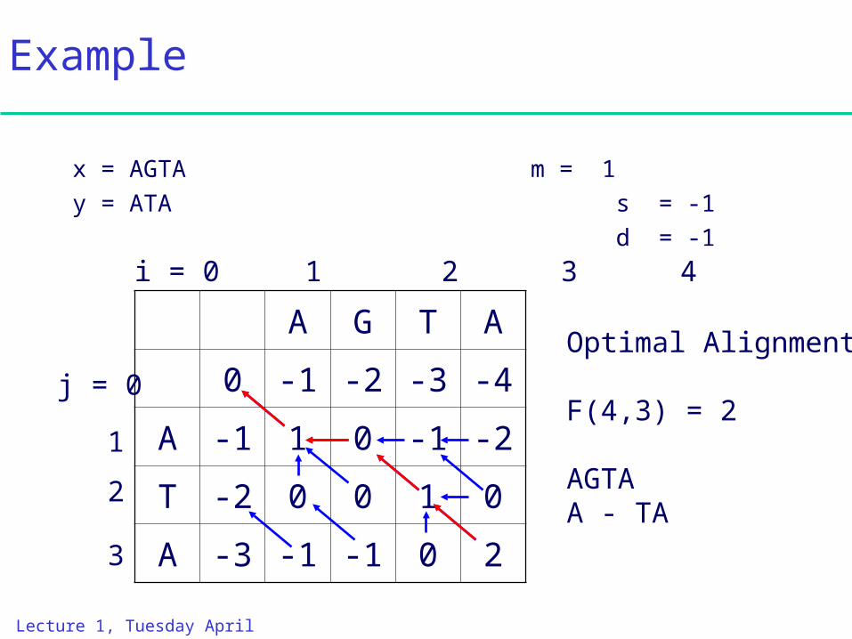
Example
x = AGTA m = 1y = ATA s = -1
d = -1
A G T A
0 -1 -2 -3 -4
A -1 1 0 -1 -2
T -2 0 0 1 0
A -3 -1 -1 0 2
F(i,j) i = 0 1 2 3 4
j = 0
1
2
3
Optimal Alignment:
F(4,3) = 2
AGTAA - TA
Lecture 1, Tuesday April 1, 2003
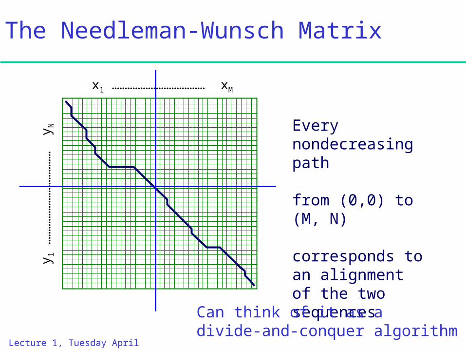
The Needleman-Wunsch Matrix
x1 ……………………………… xM
y1 …
……
……
……
……
……
…
yN
Every nondecreasing path
from (0,0) to (M, N)
corresponds to an alignment of the two sequences
Can think of it as adivide-and-conquer algorithm
Lecture 1, Tuesday April 1, 2003
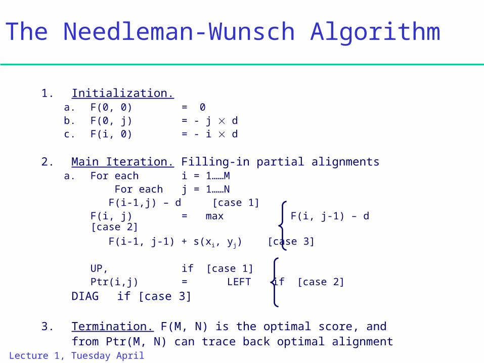
The Needleman-Wunsch Algorithm
1. Initialization.a. F(0, 0) = 0b. F(0, j) = - j dc. F(i, 0) = - i d
2. Main Iteration. Filling-in partial alignmentsa. For each i = 1……M
For each j = 1……N F(i-1,j) – d [case
1]F(i, j) = max F(i, j-1) – d [case
2] F(i-1, j-1) + s(xi, yj)
[case 3]
UP, if [case 1]Ptr(i,j) = LEFT if [case 2]
DIAG if [case 3]
3. Termination. F(M, N) is the optimal score, andfrom Ptr(M, N) can trace back optimal alignment
Lecture 1, Tuesday April 1, 2003
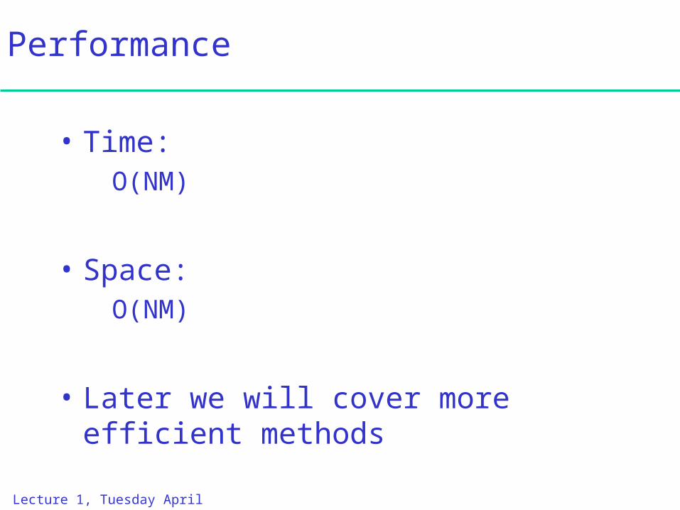
Performance
• Time:O(NM)
• Space:O(NM)
• Later we will cover more efficient methods
Lecture 1, Tuesday April 1, 2003
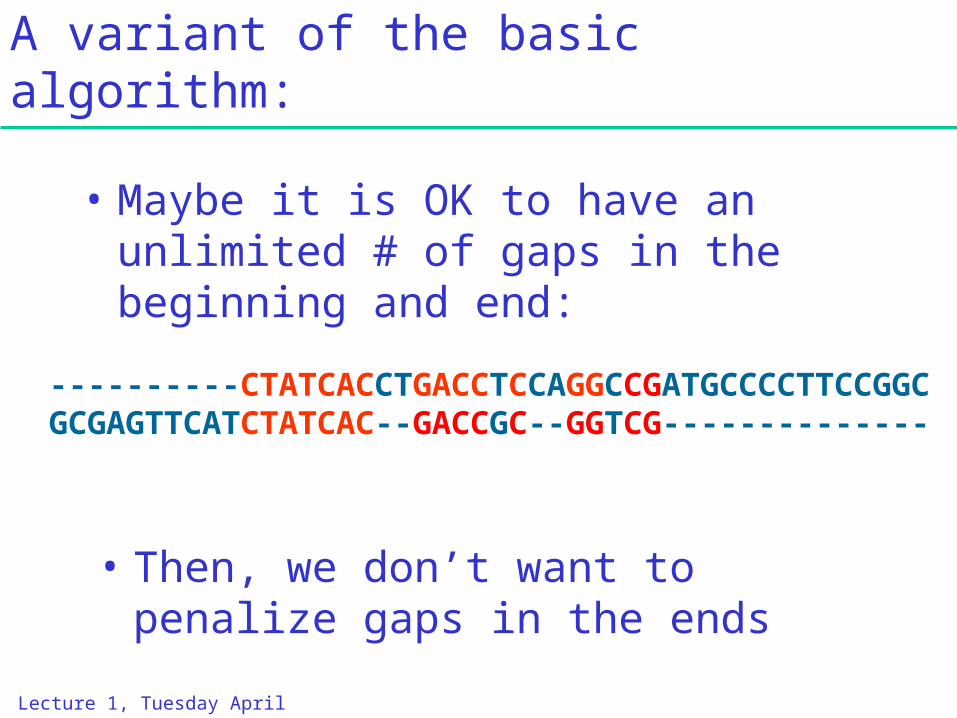
A variant of the basic algorithm:
• Maybe it is OK to have an unlimited # of gaps in the beginning and end:
----------CTATCACCTGACCTCCAGGCCGATGCCCCTTCCGGCGCGAGTTCATCTATCAC--GACCGC--GGTCG--------------
• Then, we don’t want to penalize gaps in the ends
Lecture 1, Tuesday April 1, 2003
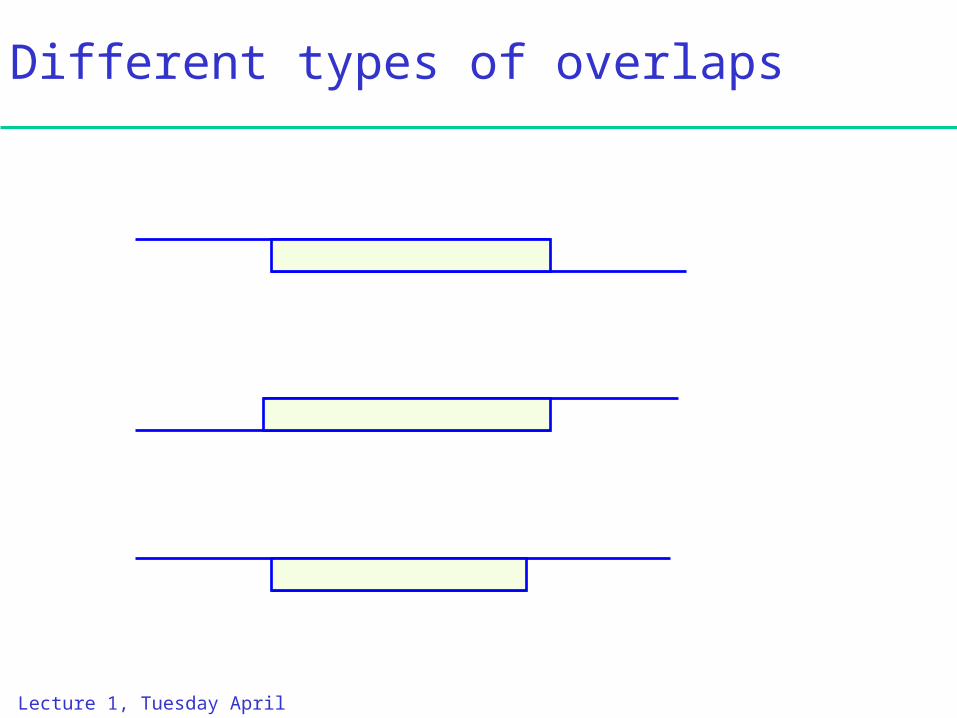
Different types of overlaps
Lecture 1, Tuesday April 1, 2003
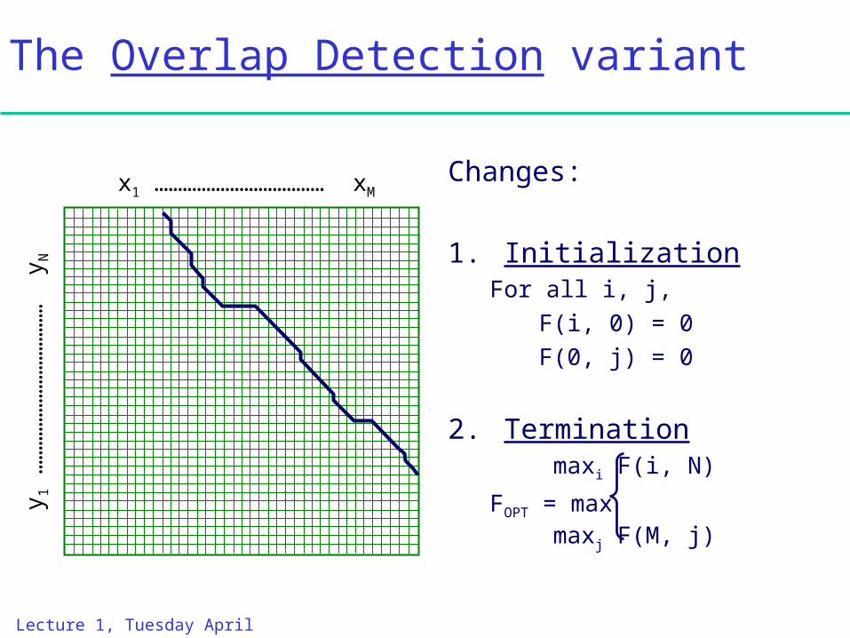
The Overlap Detection variant
Changes:
1. InitializationFor all i, j,
F(i, 0) = 0F(0, j) = 0
2. Termination maxi
F(i, N)FOPT = max
maxj F(M, j)
x1 ……………………………… xM
y1 …
……
……
……
……
……
…
yN
Lecture 1, Tuesday April 1, 2003
Next Lecture
• Local alignment
• More elaborate scoring function
• Memory-efficient algorithms
Reading:Durbin, Chapter 2
Gusfield, Chapter 11