Computational Fracture Mechanics - tf.uni-kiel.de · Computational Fracture Mechanics ......

Computational Fracture Mechanics

Summer School on

Fracture Modelling and Assessment

Wolfgang Brocks

Christian Albrecht University Kiel

Trondheim, June 2014

Part I: Fracture Concepts

(1) Linear elastic fracture mechanics (LEFM)

(2) Small scale yielding (SSY)

(3) Elastic-plastic fracture mechanics (EPFM)

Part II: Determination of Fracture Parameters

(4) FE meshes for structures with cracks

(5) CTOD, CTOA

(6) Stress intensity factors

(7) Elastic-plastic J-integral

Part III: The Cohesive Model

(8) Background - fundamentals

(9) The traction-separation law

(10) Examples, applications

(11) Cohesive elements in ABAQUS

Seite 1


Part I: Fracture Concepts

Wolfgang Brocks

Christian Albrecht University , Kiel (Germany)Materials Mechanics

(1) Linear elastic fracture mechanics (LEFM)

(2) Small Scale Yielding (SSY)

(3) Elastic-plastic fracture mechanics (EPFM)

ECF20 Trondheim 2014 2CompFractMech_01 - WB

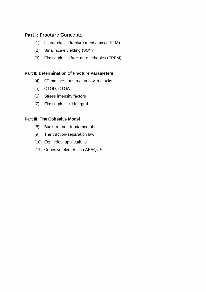
LEFM

• Stress intensity approach (IRWIN)

• Energy approach (GRIFFITH)

• J-integral

Fracture modes

Seite 2


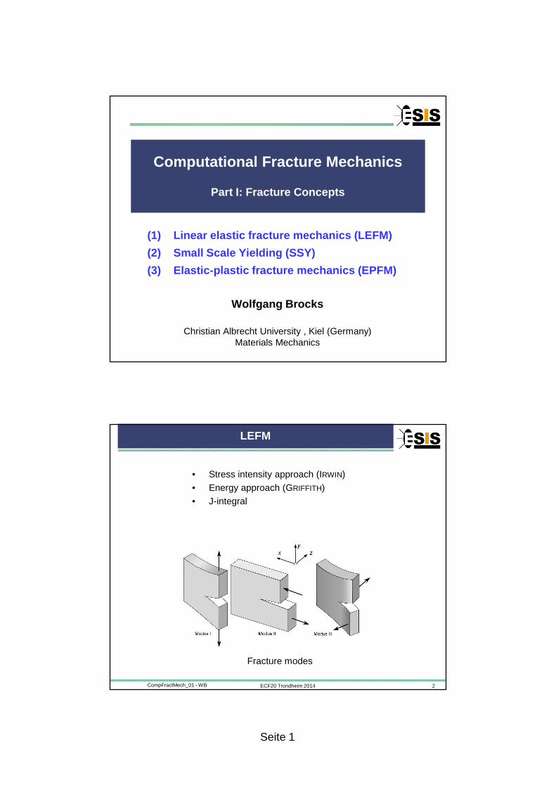
LEFM: Stress Field at a Crack Tip

IRWIN [1957]:

( ) ( ) 1 1II,

2ij ij i j

Kr f

rTσ ϑ δϑ

πδ= +

KI = stress intensity factor

T = non-singular T-stress RICE [1974]

( )I 2 geometryK a Yσ π∞=

General asymptotic solution

( ) ( ) ( ) ( )I II IIII II III

1,

2ij ij ij ijr K f K f K f

rσ ϑ ϑ ϑ ϑ

π = + + stresses

displacements ( ) ( ) ( ) ( )I II IIII II III

1,

2 2i i i i

ru r K g K g K g

Gϑ ϑ ϑ ϑ

π = + +

mode I


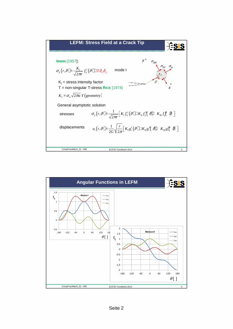
Angular Functions in LEFM

-0,5

0

0,5

1

1,5

-180 -120 -60 0 60 120 180

fij

θ [ ]

Modus I fxx

fyy

fxy

-2

-1,5

-1

-0,5

0

0,5

1

1,5

2

-180 -120 -60 0 60 120 180

fij

θ [ ]

Modus II fxx

fyy

fxy

Seite 3


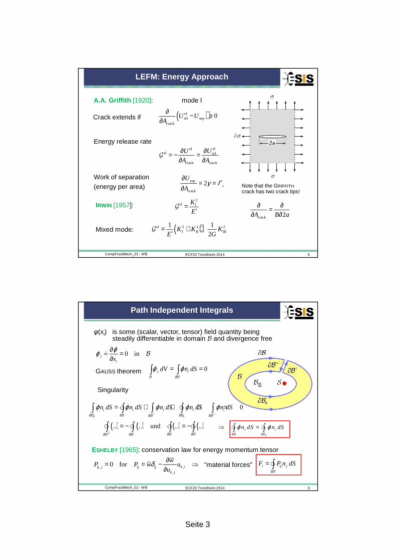
LEFM: Energy Approach

A.A. Griffith [1920]:

Crack extends if ( )elrel sep

crack

0U UA

∂ − ≥∂

Energy release rateelel

el rel

crack crack

UU

A A

∂∂= − =∂ ∂

G

Work of separation

(energy per area)sep

ccrack

2U

Aγ Γ

∂= =

∂

2el IK

E=

′GIRWIN [1957]:

Note that the GRIFFITHcrack has two crack tips!

crack 2A B a

∂ ∂=∂ ∂

Mixed mode:

mode I

( )el 2 2 2I II III

1 1

2K K K

E G= + +

′G


Path Independent Integrals

φ(xi) is some (scalar, vector, tensor) field quantity being steadily differentiable in domain B and divergence free

, 0 iniix

ϕϕ ∂ =∂≐ B

GAUSS theorem , 0i idV n dSϕ ϕ∂

= =∫ ∫B B

0 S

0ϕ ϕ ϕ ϕ ϕ− +∂ ∂ ∂∂ ∂

= + + + =∫ ∫ ∫ ∫ ∫� �i i i i in dS n dS n dS n dS n dSB B BB B

Singularity

( ) ( ) ( ) ( ).. .. und .. ..+ − ∂ ∂∂ ∂

= − = −∫ ∫ ∫ ∫� � � �B BB B

ESHELBY [1965]: conservation law for energy momentum tensor

, ,,

0 forij j ij ij k ik j

wP P w u

uδ ∂= = − ⇒

∂i ij jF P n dS

∂

= ∫�B

“material forces”

S

i in dS n dSϕ ϕ∂ ∂

⇒ =∫ ∫� �B B

Seite 4


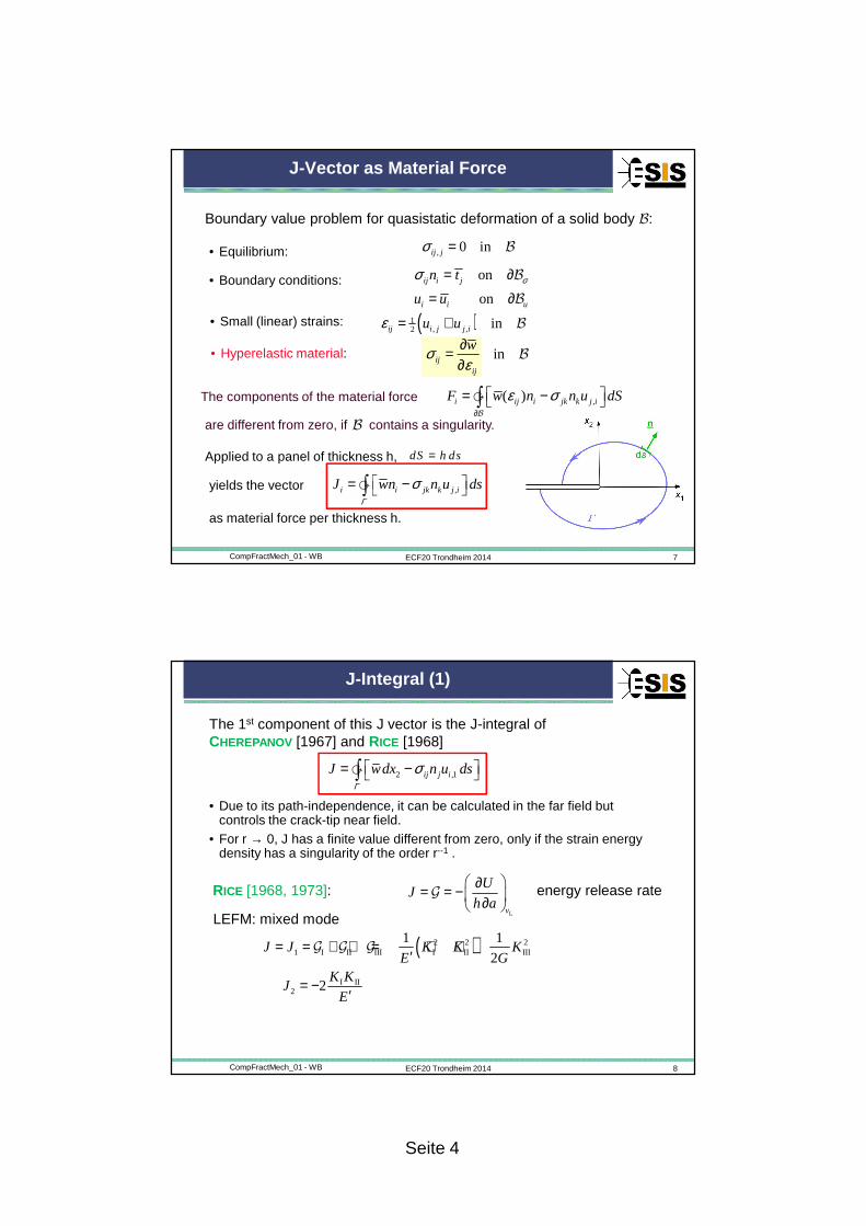
J-Vector as Material Force

• Hyperelastic material: inijij

wσε

∂=∂

B

• Equilibrium: , 0 inij jσ = B

• Boundary conditions: on

onij i j

i i u

n t

u u

σσ = ∂

= ∂

B

B

• Small (linear) strains: ( )1, ,2 inij i j j iu uε = + B

Boundary value problem for quasistatic deformation of a solid body B:

The components of the material force ,( )i ij i jk k j iF w n n u dSε σ∂

= − ∫�B

Bare different from zero, if contains a singularity.

Applied to a panel of thickness h, dS h ds=

as material force per thickness h.

,i i jk k j iJ wn n u dsΓ

σ = − ∫�yields the vector


J-Integral (1)

The 1st component of this J vector is the J-integral of CHEREPANOV [1967] and RICE [1968]

2 ,1ij j iJ wdx n u dsΓ

σ = − ∫�

• Due to its path-independence, it can be calculated in the far field but controls the crack-tip near field.

• For r → 0, J has a finite value different from zero, only if the strain energy density has a singularity of the order r--1 .

LEFM: mixed mode

( )2 2 21 I II III I II III

I II2

1 1

2

2

= = + + = + +′

= −′

J J K K KE G

K KJ

E

G G G

Lv

UJ

h a

∂= = − ∂ GRICE [1968, 1973]: energy release rate

Seite 5


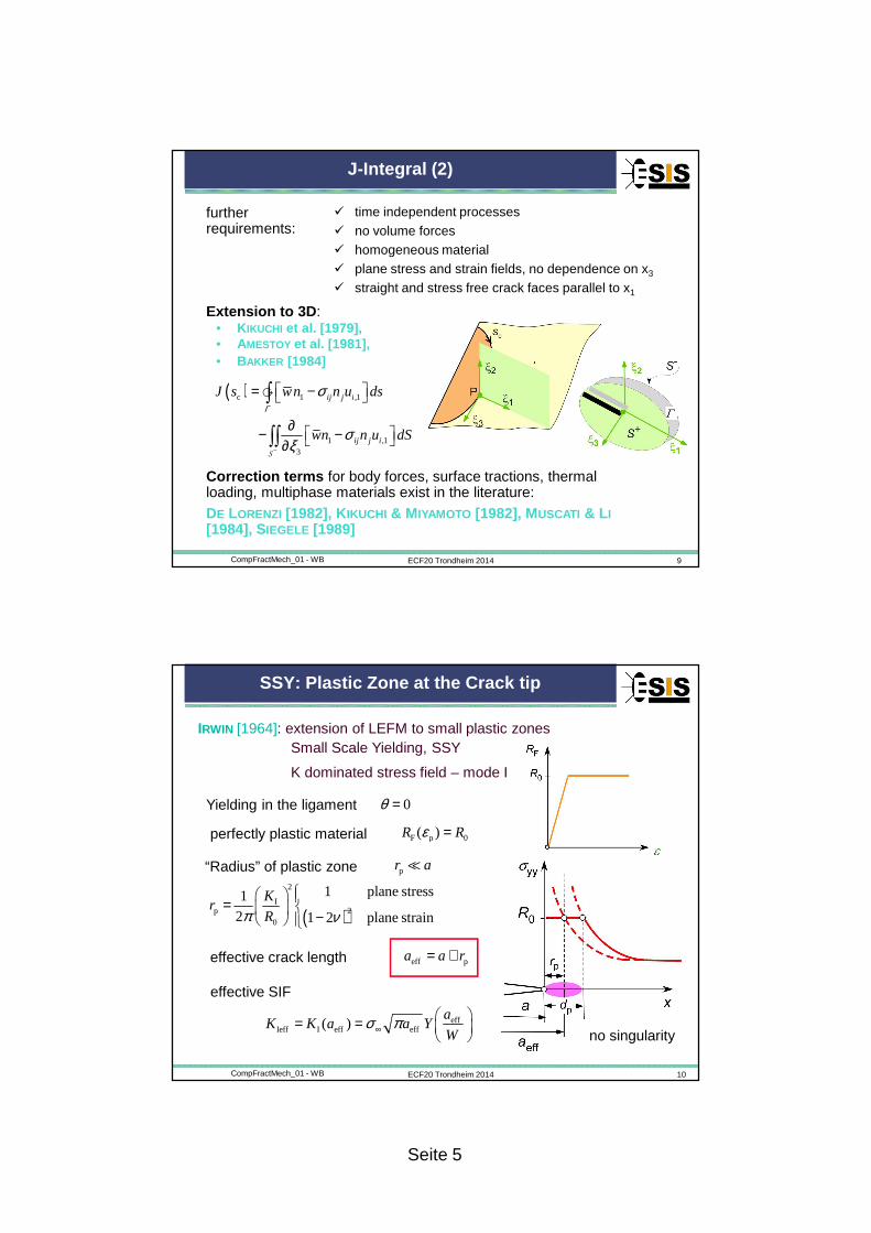
J-Integral (2)

� time independent processes� no volume forces� homogeneous material� plane stress and strain fields, no dependence on x3

� straight and stress free crack faces parallel to x1

further requirements:

Correction terms for body forces, surface tractions, thermal loading, multiphase materials exist in the literature:

DE LORENZI [1982], KIKUCHI & MIYAMOTO [1982], MUSCATI & LI[1984], SIEGELE [1989]

Extension to 3D: • KIKUCHI et al. [1979], • AMESTOY et al. [1981], • BAKKER [1984]

( )c 1 ,1

1 ,13

Γ

σ

σξ−

= −

∂ − − ∂

∫

∫∫

� ij j i

ij j i

J s wn n u ds

wn n u dSS


SSY: Plastic Zone at the Crack tip

IRWIN [1964]: extension of LEFM to small plastic zones Small Scale Yielding, SSY

K dominated stress field – mode I

0θ =Yielding in the ligament

perfectly plastic material F p 0( )R Rε =

( )

2

I2p

0

1 plane stress1

2 1 2 plane strain

Kr

Rπ ν = −

“Radius” of plastic zone pr a≪

effIeff I eff eff( )

aK K a a Y

Wσ π∞

= =

effective SIF

eff pa a r= +effective crack length

no singularity

Seite 6


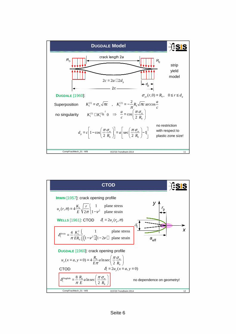
DUGDALE Model

0 p( ,0) , 0yy r R r dσ = ≤ ≤

p0 0

1 cos sec 12 2

d c aR R

π σ π σ∞ ∞

= − = −

p2 2 2c a d= +

(1) (2)I I 0

2, arccos

aK c K R c

cσ π π

π∞= = −Superposition

0

cos2

a

c R

π σ∞ ⇒ =

no singularity (1) (2)

I I 0K K+ =!

no restrictionwith respect toplastic zone size!

strip

yield

model

DUGDALE [1960]:


CTOD

I2

1 plane stress( , ) 4

1 plane strain2y

K ru r

Eπ

νπ

= −

t p2 ( , )yu rδ π=WELLS [1961]: CTOD

IRWIN [1957]: crack opening profile

0

0

( , 0) 4 lnsec2y

Ru x a y a

E R

π σπ

∞ = = =

t 2 ( , 0)yu x a yδ = = =CTOD

DUGDALE [1960]: crack opening profile

Dugdale 0t

0

8lnsec

2

Ra

E R

π σδπ

∞ =

no dependence on geometry!

( )( )2

Irwin It 2

0

1 plane stress41 1 2 plane strain

K

ERδ

ν νπ= − −

Seite 7


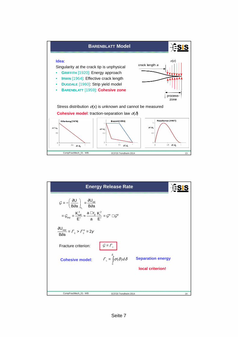
BARENBLATT Model

Idea:

Singularity at the crack tip is unphysical

• GRIFFITH [1920]: Energy approach

• IRWIN [1964]: Effective crack length

• DUGDALE [1960]: Strip yield model

• BARENBLATT [1959]: Cohesive zone

Stress distribution σ(x) is unknown and cannot be measured

Cohesive model: traction-separation law σ(δ)


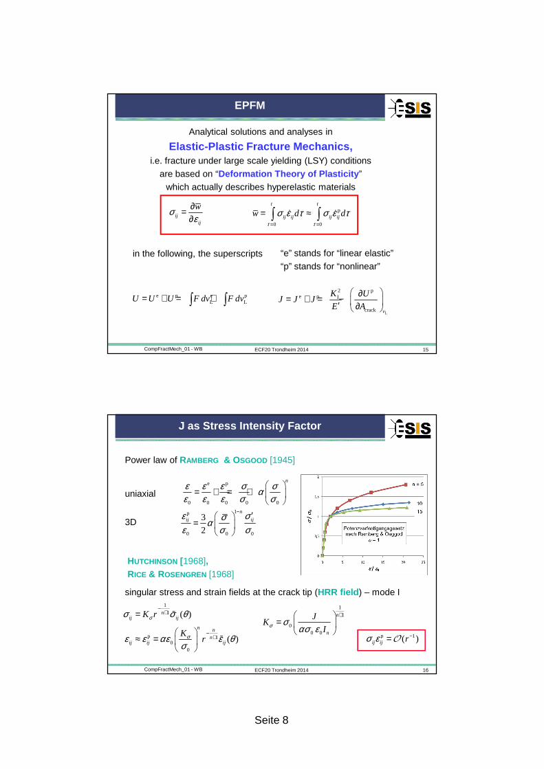
Energy Release Rate

∂∂ = − = ∂ ∂

+= = ≈ = +

′ ′

G

G G G

L

rel

2 2p e pIeff I

ssy

v

UUB a B a

a rK KE a E

Γ Γ γ∂

= > =∂sep e

c c 2U

B a

Separation energyCohesive model:c

c

0

( )dδ

Γ σ δ δ= ∫

cΓ=GFracture criterion:

local criterion!

Seite 8


EPFM

Analytical solutions and analyses in

Elastic-Plastic Fracture Mechanics,i.e. fracture under large scale yielding (LSY) conditions

are based on “Deformation Theory of Plasticity”

which actually describes hyperelastic materials

ijij

wσε

∂=∂

p

0 0

t t

ij ij ij ijw d dτ τ

σ ε τ σ ε τ= =

= ≈∫ ∫ɺ ɺ

“e” stands for “linear elastic”

“p” stands for “nonlinear”

e p e pL LU U U F dv F dv= + = +∫ ∫

L

2 pe p I

crack v

K UJ J J

E A

∂= + = − ′ ∂

in the following, the superscripts


J as Stress Intensity Factor

Power law of RAMBERG & OSGOOD [1945]

e p

0 0 0 0 0

nε ε ε σ σαε ε ε σ σ

= + = +

uniaxial

1p

0 0 0

3

2

n

ij ijε σσαε σ σ

− ′ =

3D

HUTCHINSON [1968], RICE & ROSENGREN [1968]

singular stress and strain fields at the crack tip (HRR field) – mode I1

1

p 10

0

( )

( )

nij ij

n n

nij ij ij

K r

Kr

σ

σ

σ σ θ

ε ε αε ε θσ

−+

−+

=

≈ =

ɶ

ɶ

1

1

00 0

n

n

JK

Iσ σασ ε

+ =

p 1( )ij ij rσ ε −=O

Seite 9


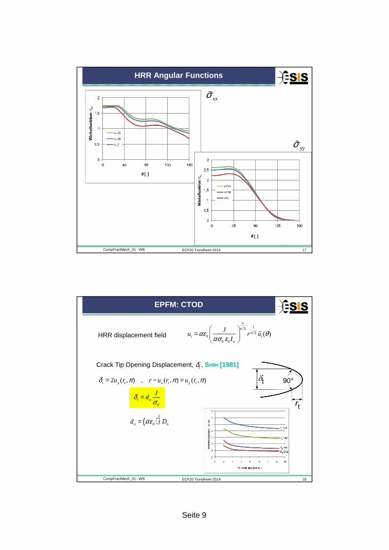
HRR Angular Functions

xxσɶ

yyσɶ


EPFM: CTOD

HRR displacement field11

10

0 0

( )

n

nn

i in

Ju r u

Iαε θ

ασ ε+

+

=

ɶ

Crack Tip Opening Displacement, δt , SHIH [1981]

t t t t2 ( , ) , ( , ) ( , )y x yu r r u r u rδ π π π= − =

t0

n

Jdδ

σ=

( )1

0n

n nd Dαε=

Seite 10


Path Dependence of J

FE simulationC(T) specimen

plane strain

stationary crack

incremental theoryof plasticity

ASTM E 1820: reference value

“far field” value

e pJ J J= +2

e IKJ

E=

′( )IK a Y a Wσ π∞=

( )p

p UJ

B W a

η=−


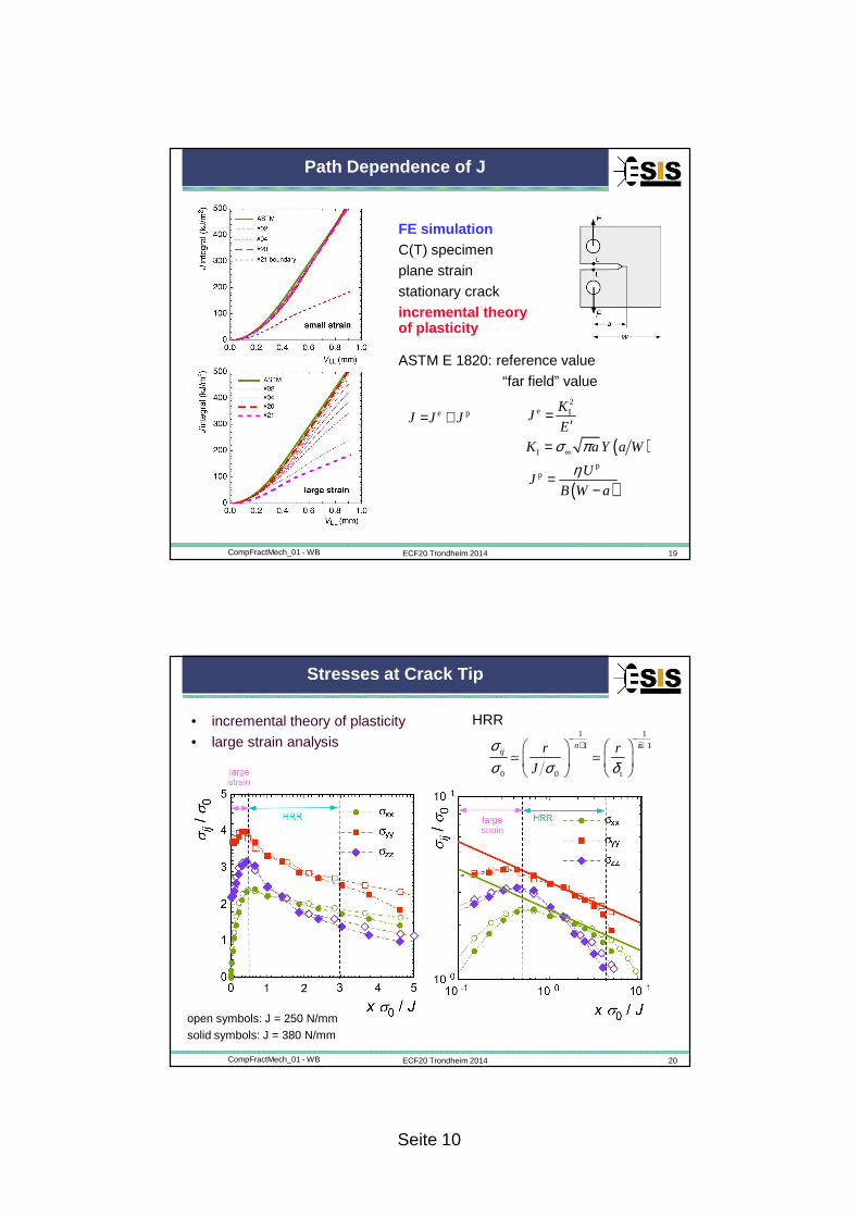
Stresses at Crack Tip

• incremental theory of plasticity

• large strain analysis1 1

1 1

0 0 t

n nij r r

J

σσ σ δ

− −+ +

≃ ≃

HRR

open symbols: J = 250 N/mmsolid symbols: J = 380 N/mm

Seite 11


Literature

W. BROCKS, A. CORNEC, I. SCHEIDER: Computational Aspects of Nonlinear Fracture Mechanics. In: I. Milne, R.O. Ritchie, B. Karihaloo(Eds.): Comprehensive Structural Integrity - Numerical and Computational Methods. Vol. 3, Oxford: Elsevier, 2003. 127 - 209. (ISBN: 0-08-043749-4)

W. BROCKS: Computational Fracture Mechanics. In: D. RAABE, F. ROTERS, F. BARLAT, L.-Q. CHEN (Eds.): Continuum Scale Simulation of Engineering Materials. Weinheim: WILEY-VCH, 2004. 621 - 637

W. BROCKS, W.: Computational Fracture Mechanics. In: R. BLOCKLEY, W. SHYY (Eds.): Encyclopedia of Aerospace Engineering, Vol. 3, John Wiley & Sons, 2010.

M. KUNA: Finite Elements in Fracture Mechanics, Springer Dordrecht, 2013. (ISBN 978-94-007-6679-2)

Seite 1


Part II: Determination of Fracture Parameters

Wolfgang Brocks


(1) FE meshes for structures with cracks

(2) CTOD, CTOA

(3) Stress intensity factors

(4) Elastic-plastic J-integral


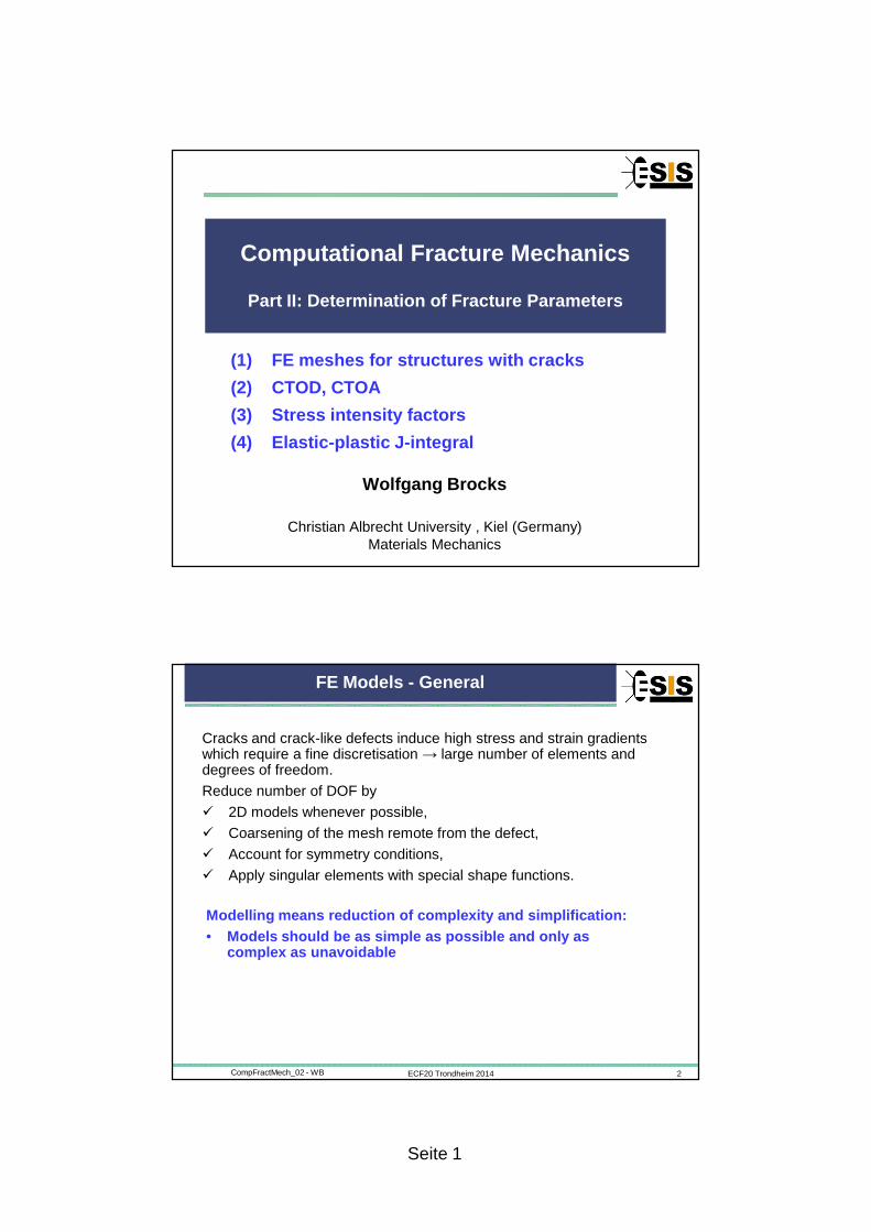
FE Models - General

Cracks and crack-like defects induce high stress and strain gradients which require a fine discretisation → large number of elements and degrees of freedom.

Reduce number of DOF by

� 2D models whenever possible,

� Coarsening of the mesh remote from the defect,

� Account for symmetry conditions,

� Apply singular elements with special shape functions.

Modelling means reduction of complexity and simplifi cation:• Models should be as simple as possible and only as

complex as unavoidable

Seite 2


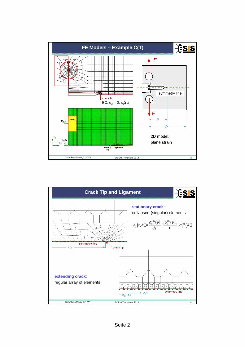
FE Models – Example C(T)

symmetry line

2D model:

plane strain

BC: u2 = 0, x1≥ a


Crack Tip and Ligament

stationary crack :

collapsed (singular) elements

extending crack :

regular array of elements

( ) ( ) ( ) ( )(0) (1)

(2), ij ijij ijr

rr

α ϑ α ϑε ϑ α ϑ= + +

Seite 3


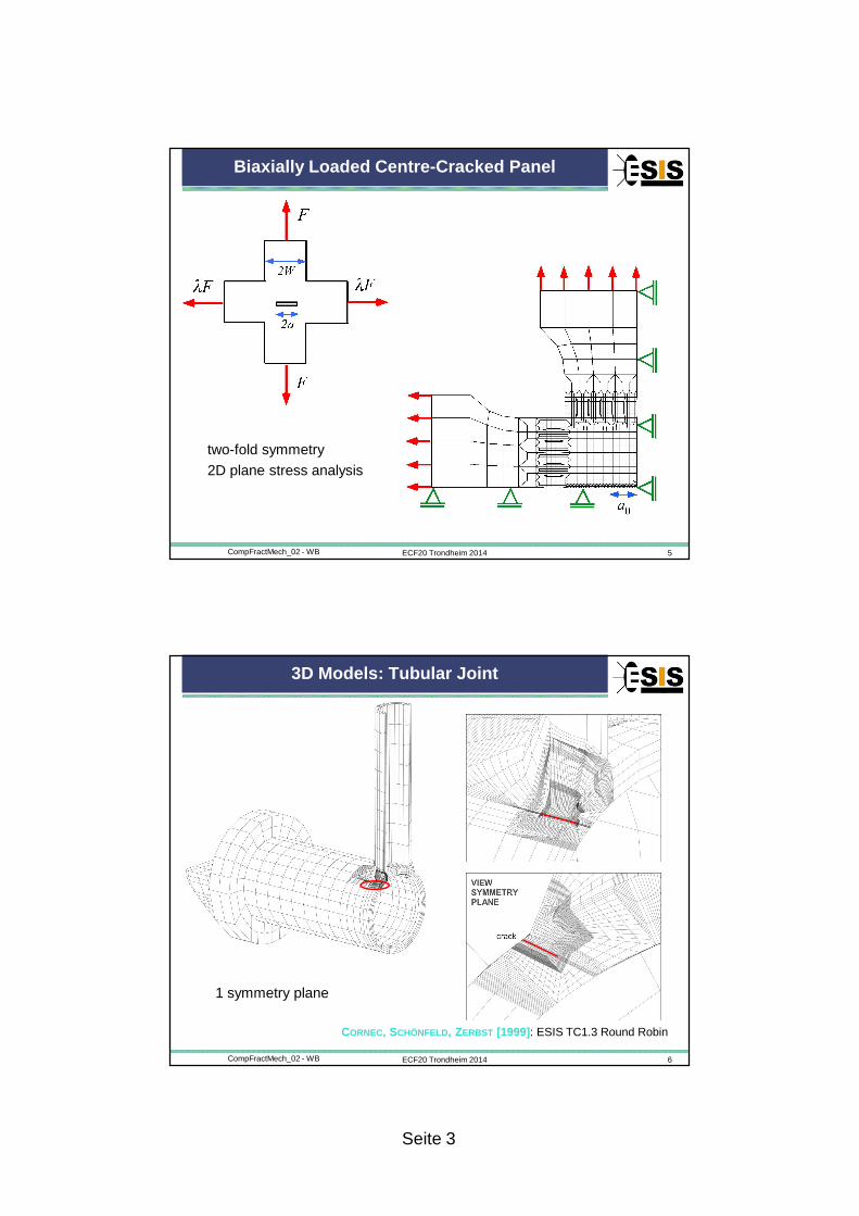
Biaxially Loaded Centre-Cracked Panel

two-fold symmetry

2D plane stress analysis


3D Models: Tubular Joint

CORNEC, SCHÖNFELD, ZERBST [1999] : ESIS TC1.3 Round Robin

1 symmetry plane

Seite 4


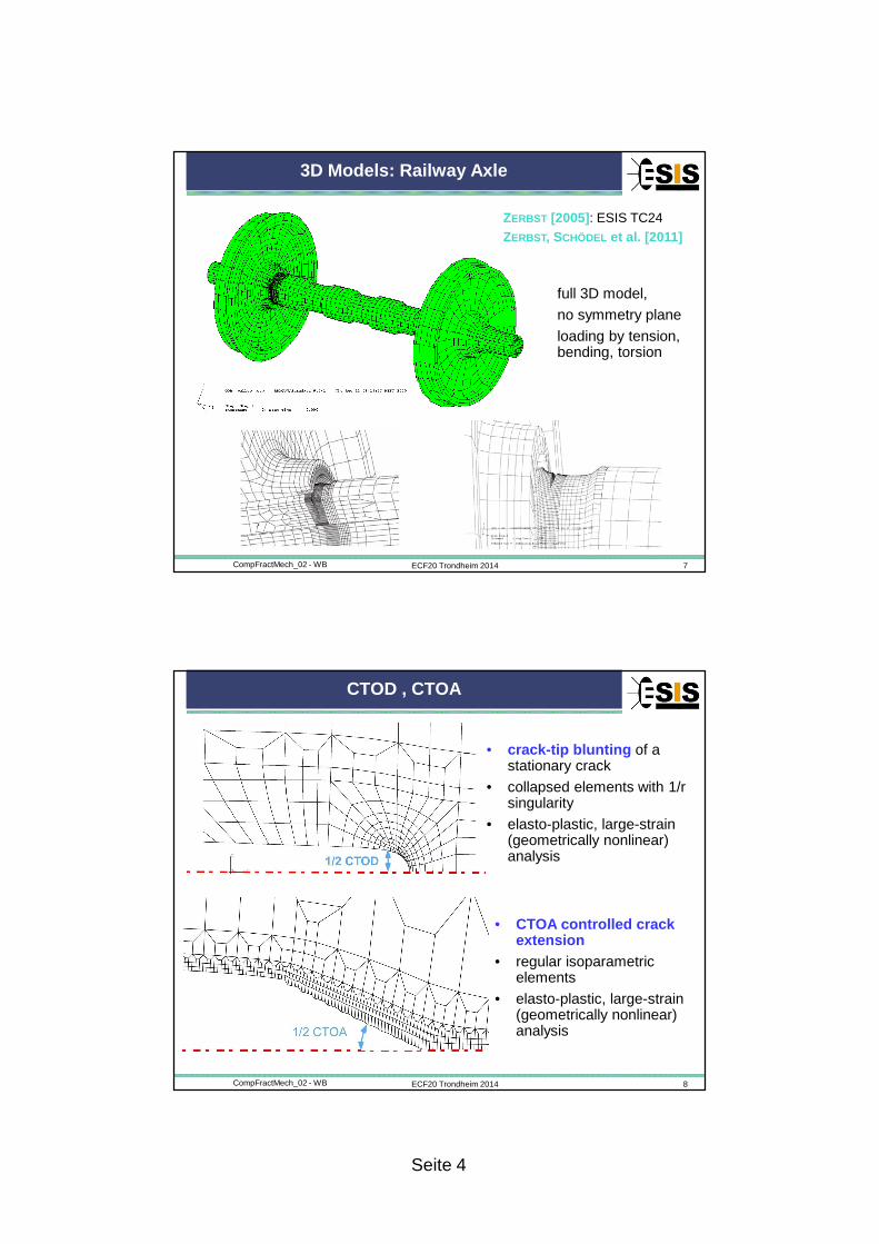
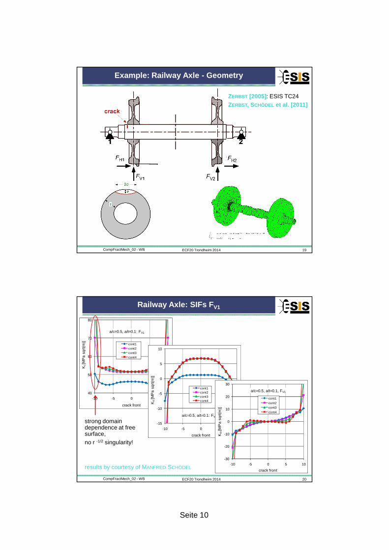
3D Models: Railway Axle

ZERBST [2005]: ESIS TC24ZERBST, SCHÖDEL et al. [2011]

full 3D model,

no symmetry plane

loading by tension, bending, torsion


CTOD , CTOA

• crack-tip blunting of a stationary crack

• collapsed elements with 1/rsingularity

• elasto-plastic, large-strain (geometrically nonlinear) analysis

• CTOA controlled crack extension

• regular isoparametricelements

• elasto-plastic, large-strain (geometrically nonlinear) analysis

Seite 5


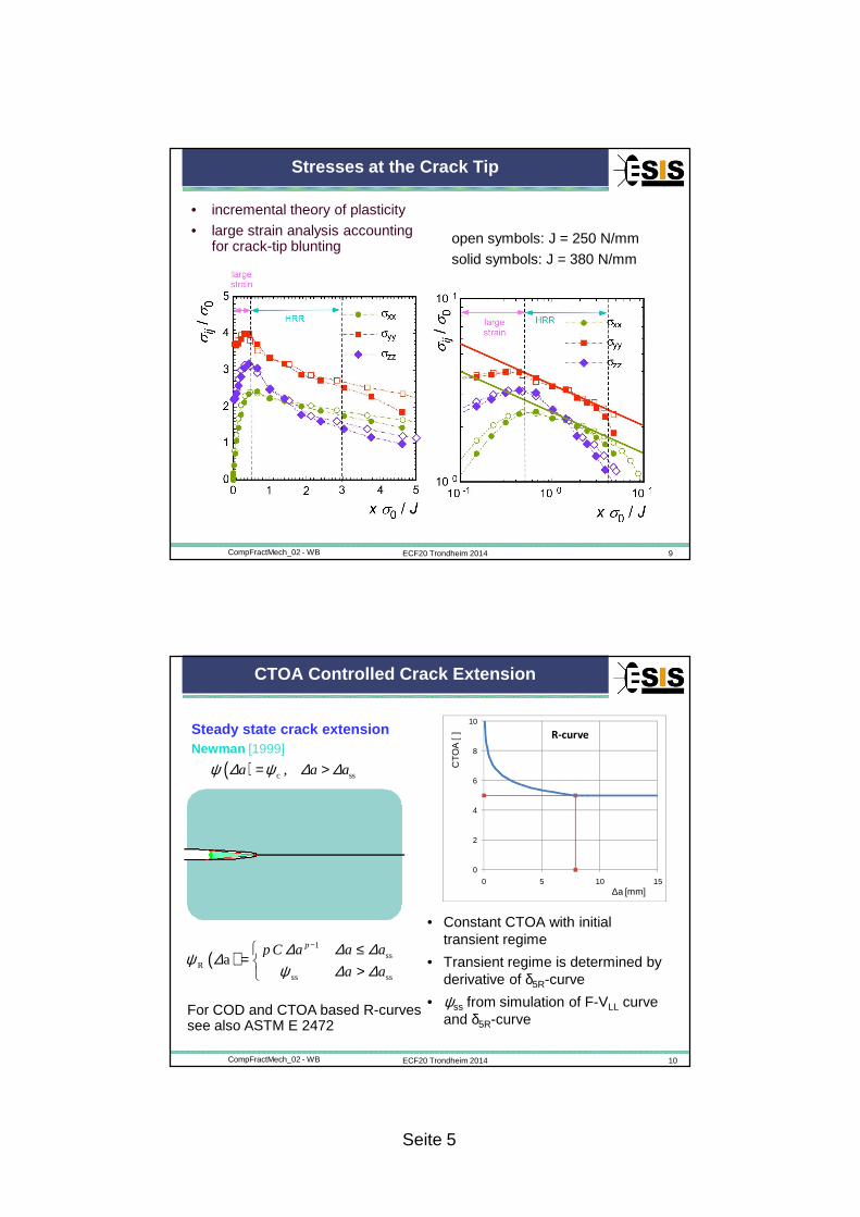
Stresses at the Crack Tip

• incremental theory of plasticity

• large strain analysis accounting for crack-tip blunting open symbols: J = 250 N/mm

solid symbols: J = 380 N/mm


CTOA Controlled Crack Extension

Steady state crack extensionNewman [1999]

( ) c ss,a a aψ ∆ ψ ∆ ∆= >

• Constant CTOA with initial transient regime

• Transient regime is determined by derivative of δ5R-curve

• ψss from simulation of F-VLL curve and δ5R-curve

( )1

ssR

ss ss

app C a a a

a a

∆ ∆ ∆ψ ∆ψ ∆ ∆

− ≤= >

0

2

4

6

8

10

0 5 10 15

CTO

A [

]

∆a [mm]

R-curve

For COD and CTOA based R-curves see also ASTM E 2472

Seite 6


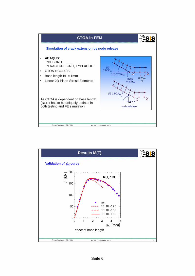
CTOA in FEM

• ABAQUS :*DEBOND*FRACTURE CRIT, TYPE=COD

• CTOA = COD / BL

• Base length BL = 1mm

• Linear 2D Plane Stress Elements

a

1/2 CTOAFE

node release

1/2 CTOAFE

1/2 CTODFE

base lengthFE

0,25mm

Simulation of crack extension by node release

As CTOA is dependent on base length (BL), it has to be uniquely defined in both testing and FE simulation


Results M(T)

Validation of ψR-curve

effect of base length

Seite 7


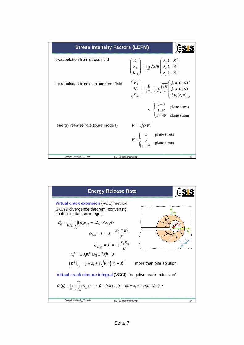
Stress Intensity Factors (LEFM)

3plane stress

13 4 plane strain

νκ ν

ν

−= + −

I

II0

III

( ,0)

lim 2 ( ,0)

( ,0)

σπ σ

σ→

=

yy

xyr

yz

K r

K r r

K r

extrapolation from stress field

1I 1

1II 10

1III 4

( , )2

lim ( , )1

( , )

κ

κ

ππ π

νπ

+

+→

= +

y

xr

z

K u rE

K u rr

K u r

extrapolation from displacement field

energy release rate (pure mode I)I ′=K EG

2

plane stress

plane strain1 ν

′ = −

EE E


Energy Release Rate

( )0

, ,

1ϕ σ δ ∆

∆= −∫∫ ij j k ik k iu w x dS

h aB

G

2 2I II

0 1ϕ=+= = =

′K K

J JE

G

I II2

22πϕ =

= = −′

K KJ

EG

Virtual crack extension (VCE) method

GAUSS’ divergence theorem: converting contour to domain integral

1I 20

0

( ) lim ( , 0, ) ( , , )dδ

δσ ϑ δ ϑ π δ

→=

= = = = − = +∫a

yy ya

x

a r x a u r a x a a xG

Virtual crack closure integral (VCCI): “negative crack extension”

4 2 2 21I 1 I 24 0K E J K E J′ ′− + =

( ) ( )2 2 2 21 1I 1 1 22 21,2

K E J E J J′ ′= ± − more than one solution!

Seite 8


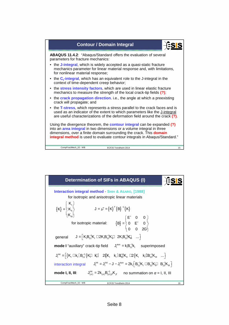
Contour / Domain Integral

ABAQUS 11.4.2 : “Abaqus/Standard offers the evaluation of several parameters for fracture mechanics:

• the J-integral , which is widely accepted as a quasi-static fracture mechanics parameter for linear material response and, with limitations, for nonlinear material response;

• the Ct-integral , which has an equivalent role to the J-integral in the context of time-dependent creep behavior;

• the stress intensity factors , which are used in linear elastic fracture mechanics to measure the strength of the local crack-tip fields (?);

• the crack propagation direction . i.e., the angle at which a preexisting crack will propagate; and

• the T-stress , which represents a stress parallel to the crack faces and is used as an indicator of the extent to which parameters like the J-integral are useful characterizations of the deformation field around the crack (?).

Using the divergence theorem, the contour integral can be expanded (?) into an area integral in two dimensions or a volume integral in three dimensions, over a finite domain surrounding the crack. This domain integral method is used to evaluate contour integrals in Abaqus/Standard.”


Determination of SIFs in ABAQUS (I)

Interaction integral method - SHIH & ASARO, [1988]for isotropic and anisotropic linear materials

{ }I

II

III

K

K

K

K

=

{ } { } { }T 1K B KJ

−= =G

for isotropic material: { }0 0

B 0 0

0 0 2

E

E

G

′ ′=

general 1 1 1I 11 I I 12 II I 13 III2 2 ...J K B K K B K K B K− − − = + + +

superimposedmode I “auxiliary” crack-tip field aux 1I I 11 IJ k B k−=

( ) ( ) ( ) ( )tot 1 1 1I I I 11 I I I I 12 II I I 13 III2 2 ...J K k B K k K k B K K k B K− − − = + + + + + + +

interaction integral int tot aux 1 1 1I I I I 11 I 12 II 13 III2J J J J k B K B K B K− − − = − − = + +

mode I, II, III : int 1( ) ( ) ( )2J k B Kα α α β β

−= no summation on α = I, II, III

Seite 9


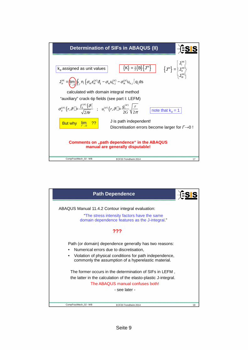
Determination of SIFs in ABAQUS (II)

( )int ( ) ( ) ( ), ,0

lim i kl kl ij ik k j ik k j jJ n u u q dsα α αα ΓΓ

σ ε δ σ σ→

= − −∫�

calculated with domain integral method

kα assigned as unit values { } { }{ }int12K B J= { }

intI

int intIIintIII

J

J

J

J

=

But why0

limΓ →

?? J is path independent!

Discretisation errors become larger for Γ→0 !

Comments on „path dependence“ in the ABAQUS manual are generally disputable!

“auxiliary” crack-tip fields (see part I: LEFM)

( ) ( ) ( )( ) ( )

( ) ( ), ; ,2 22

α αα αϑ

σ ϑ ϑππ

= =ij iij i

f g rr u r

Gr note that kα = 1


Path Dependence

“The stress intensity factors have the same domain dependence features as the J-integral.”

ABAQUS Manual 11.4.2 Contour integral evaluation:

???

Path (or domain) dependence generally has two reasons:

• Numerical errors due to discretisation,

• Violation of physical conditions for path independence, commonly the assumption of a hyperelastic material.

The former occurs in the determination of SIFs in LEFM ,

the latter in the calculation of the elasto-plastic J-integral.

The ABAQUS manual confuses both!

- see later -

Seite 10


Example: Railway Axle - Geometry

ZERBST [2005]: ESIS TC24ZERBST, SCHÖDEL et al. [2011]


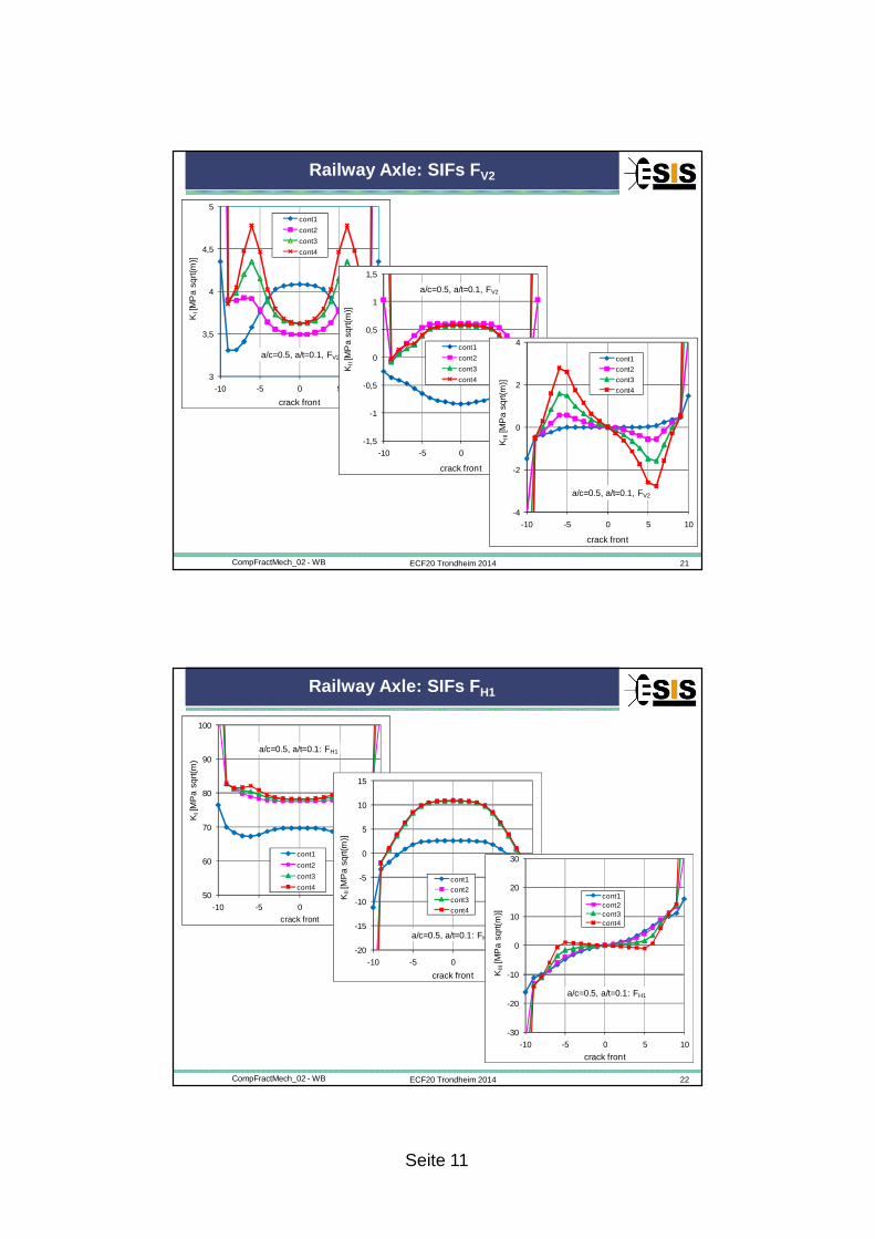
Railway Axle: SIFs FV1

40

50

60

70

80

-10 -5 0 5 10

KI[

MP

a sq

rt(m

)]

crack front

a/c=0.5, a/t=0.1: FV1

cont1cont2cont3cont4

-15

-10

-5

0

5

10

-10 -5 0 5 10

KII

[MP

a s

qrt(m

)]

crack front

a/c=0.5, a/t=0.1: FV1


-30

-20

-10

0

10

20

30

-10 -5 0 5 10

KIII

[MP

a sq

rt(m

)]

crack front

a/c=0.5, a/t=0.1, FV1

cont1

cont2cont3

cont4

strong domain dependence at free surface,no r -1/2 singularity!

results by courtesy of MANFRED SCHÖDEL

Seite 11


Railway Axle: SIFs FV2

3

3,5

4

4,5

5

-10 -5 0 5 10

KI[

MP

a sq

rt(m

)]

crack front

a/c=0.5, a/t=0.1, FV2

cont1

cont2

cont3

cont4

-1,5

-1

-0,5

0

0,5

1

1,5

-10 -5 0 5 10

KII

[MP

a sq

rt(m

)]

crack front

a/c=0.5, a/t=0.1, FV2

cont1

cont2

cont3

cont4

-4

-2

0

2

4

-10 -5 0 5 10

KIII

[MP

a sq

rt(m

)]

crack front

a/c=0.5, a/t=0.1, FV2

cont1

cont2

cont3

cont4


Railway Axle: SIFs FH1

50

60

70

80

90

100

-10 -5 0 5 10

KI[

MP

a sq

rt(m

)

crack front

a/c=0.5, a/t=0.1: FH1

cont1

cont2

cont3

cont4

-20

-15

-10

-5

0

5

10

15

-10 -5 0 5 10

KII

[MP

a sq

rt(m

)]

crack front

a/c=0.5, a/t=0.1: FH1

cont1cont2cont3

cont4

-30

-20

-10

0

10

20

30

-10 -5 0 5 10

KIII

[MP

a s

qrt(m

)]

crack front

a/c=0.5, a/t=0.1: FH1


Seite 12


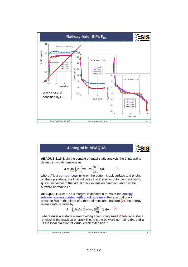
Railway Axle: SIFs FH2

-150

-125

-100

-75

-50

-10 -5 0 5 10

KI[

MP

a sq

rt(m

)]

crack front

a/c=0.5, a/t=0.1: FH2


crack closure!

condition KI > 0-20

-10

0

10

20

30

40

-10 -5 0 5 10

KII

[MP

a sq

rt(m

)]

crack front

a/c=0.5, a/t=0.1: FH2

cont1

cont2

cont3

cont4

-30

-20

-10

0

10

20

30

-10 -5 0 5 10

KIII

[MP

a sq

rt(m

)]

crack front

a/c=0.5, a/t=0.1: FH2

cont1

cont2

cont3

cont4


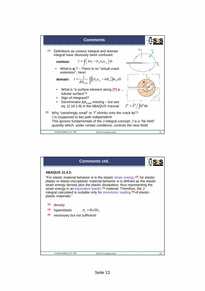
J-Integral in ABAQUS

ABAQUS 11.4.2 : “The J-integral is defined in terms of the energy release rate associated with crack advance . For a virtual crack advance λ(s) in the plane of a three-dimensional fracture (?), the energy release rate is given by

where dA is a surface element along a vanishing small (2) tubular surface enclosing the crack tip or crack line, n is the outward normal to dA, and qis the local direction of virtual crack extension. “

( )A

J s w dAλ ∂ = ⋅ − ⋅ ⋅ ∂ ∫

un I σ q

x(1)

ABAQUS 2.16.1 : „In the context of quasi-static analysis the J-integral is defined in two dimensions as

where Γ is a contour beginning on the bottom crack surface and ending on the top surface, the limit indicates that Γ shrinks onto the crack tip (2); q is a unit vector in the virtual crack extension direction; and n is the outward normal to Γ.“

0limJ w d

ΓΓΓ

→

∂ = ⋅ − ⋅ ⋅ ∂ ∫

un I σ q

x(1)

Seite 13


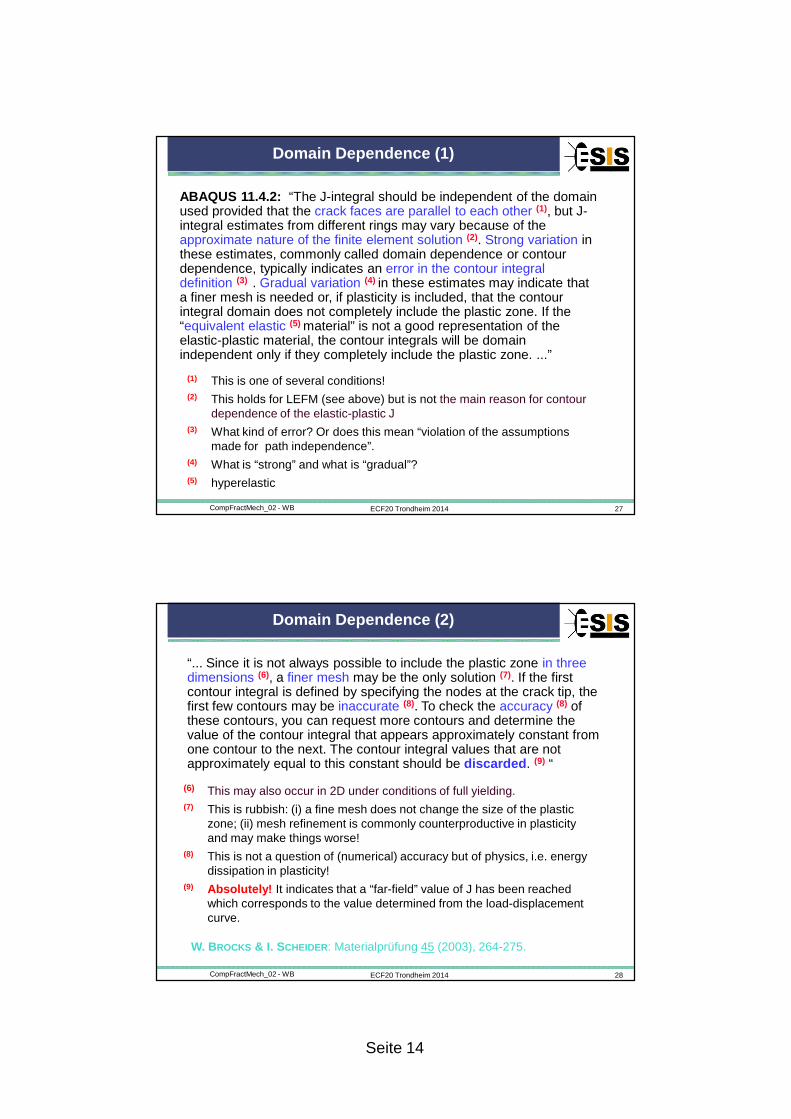
Comments

(1) Definitions as contour integral and domain integral have obviously been confused.

(2) Why “vanishingly small” or “Γ shrinks onto the crack tip”? J is (supposed to be) path independent! This ignores fundamentals of the J-integral concept: J is a “far-field” quantity which, under certain conditions, controls the near-field!

• What is q ? – There is no “virtual crack extension”, here!

1 ,1

Γ

σ = − ∫� jk k jJ wn n u dscontour :

• What is “a surface element along (?) a … tubular surface”?

• Sign of integrand?• Denominator ∆Acrack missing – but see

eq. (2.16.1-9) in the ABAQUS manual:

( )0

,1 1 1,crack

1 σ δ ∆∆

= −∫∫ ij j i iJ u w x dSA

B

domain :

P P PJ J N ds= ∫


Comments ctd.

ABAQUS 11.4.2:“For elastic material behavior w is the elastic strain energy (3); for elastic-plastic or elasto-viscoplastic material behavior w is defined as the elastic strain energy density plus the plastic dissipation, thus representing the strain energy in an equivalent elastic (4) material. Therefore, the J-integral calculated is suitable only for monotonic loading (5) of elastic-plastic materials.”

(3) density(4) hyperelastic(5) necessary but not sufficient!

σ ε= ∂ ∂ij ijw

Seite 14


Domain Dependence (1)

ABAQUS 11.4.2: “The J-integral should be independent of the domain used provided that the crack faces are parallel to each other (1), but J-integral estimates from different rings may vary because of the approximate nature of the finite element solution (2). Strong variation in these estimates, commonly called domain dependence or contour dependence, typically indicates an error in the contour integral definition (3) . Gradual variation (4) in these estimates may indicate that a finer mesh is needed or, if plasticity is included, that the contour integral domain does not completely include the plastic zone. If the “equivalent elastic (5) material” is not a good representation of the elastic-plastic material, the contour integrals will be domain independent only if they completely include the plastic zone. ...”

(1) This is one of several conditions!(2) This holds for LEFM (see above) but is not the main reason for contour

dependence of the elastic-plastic J(3) What kind of error? Or does this mean “violation of the assumptions

made for path independence”.(4) What is “strong” and what is “gradual”?(5) hyperelastic


Domain Dependence (2)

“... Since it is not always possible to include the plastic zone in three dimensions (6), a finer mesh may be the only solution (7). If the first contour integral is defined by specifying the nodes at the crack tip, the first few contours may be inaccurate (8). To check the accuracy (8) of these contours, you can request more contours and determine the value of the contour integral that appears approximately constant from one contour to the next. The contour integral values that are not approximately equal to this constant should be discarded . (9) “

(6) This may also occur in 2D under conditions of full yielding.(7) This is rubbish: (i) a fine mesh does not change the size of the plastic

zone; (ii) mesh refinement is commonly counterproductive in plasticity and may make things worse!

(8) This is not a question of (numerical) accuracy but of physics, i.e. energy dissipation in plasticity!

(9) Absolutely! It indicates that a “far-field” value of J has been reached which corresponds to the value determined from the load-displacement curve.

W. BROCKS & I. SCHEIDER: Materialprüfung 45 (2003), 264-275.

Seite 15


J Calculation

ABAQUS/Standard uses the domain integral method to evaluate the J-integral and automatically finds the elements that form each ring from the regions defined as the crack tip or crack line.

Each contour provides an evaluation of the contour integral. The number , n, of contours must be specified in the history output request.

*CONTOUR INTEGRAL, CONTOURS=n, TYPE=J

• Defining the crack front

• Specifying the virtual crack extension direction


Defining the Crack Front

*CONTOUR INTEGRAL, CONTOURS=n, CRACK TIP NODESSpecify the crack front node set name and the crack tip node number or node set name.

The user must specify the crack front , i.e., the region that defines the first contour . ABAQUS/Standard uses this region and one layer of elements surrounding it to compute the first contour integral. An additional layer of elements is used to compute each subsequent contour. The crack front can be equal to the crack tip in two dimensions or it can be a larger region surrounding the crack tip, in which case it must include the crack tip. By default ABAQUS defines the crack tip as the node specified for the crack front in the so called CRACK TIP NODES option of the contour integral command:

Alternatively, a user-defined node set which include the crack tip can be provided to ABAQUS manually by omitting the crack tip nodes option:

*CONTOUR INTEGRAL, CONTOURS=nSpecify the crack front node set name and the crack tip node number or node set name.

Seite 16


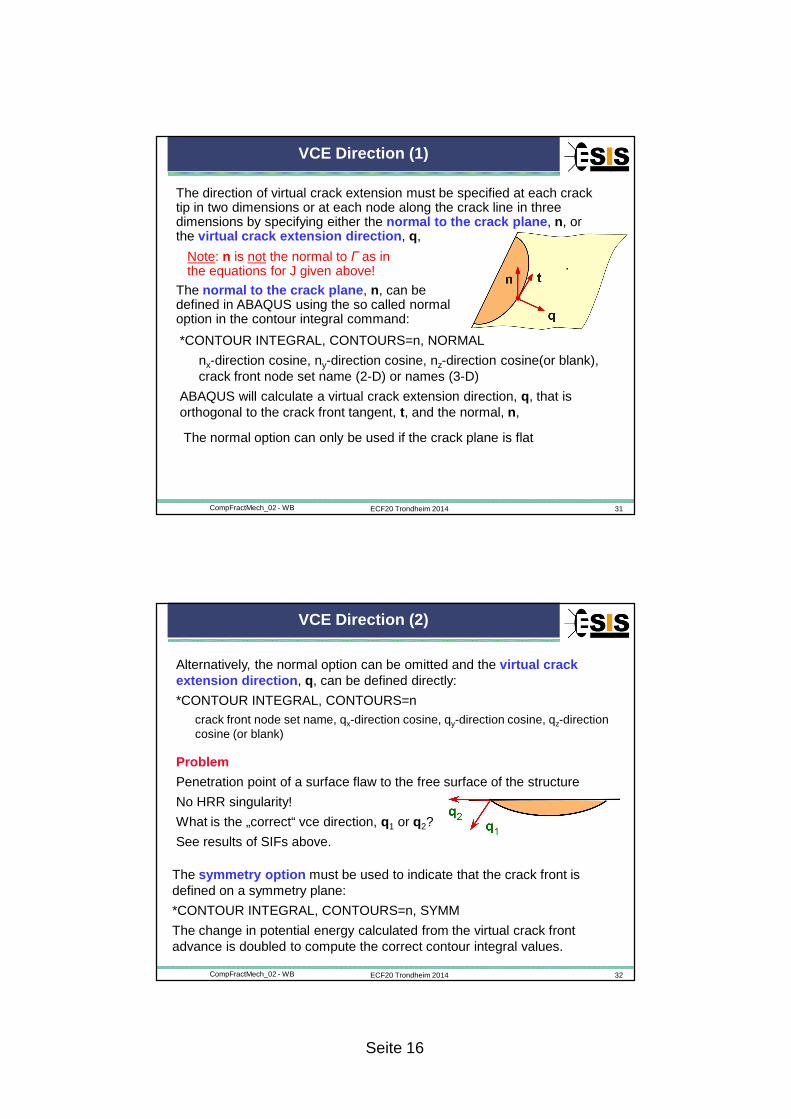
VCE Direction (1)

The direction of virtual crack extension must be specified at each crack tip in two dimensions or at each node along the crack line in three dimensions by specifying either the normal to the crack plane , n, or the virtual crack extension direction , q,

Note: n is not the normal to Γ as in the equations for J given above!

*CONTOUR INTEGRAL, CONTOURS=n, NORMAL

nx-direction cosine, ny-direction cosine, nz-direction cosine(or blank), crack front node set name (2-D) or names (3-D)

ABAQUS will calculate a virtual crack extension direction, q, that is orthogonal to the crack front tangent, t, and the normal, n,

The normal to the crack plane , n, can be defined in ABAQUS using the so called normal option in the contour integral command:

The normal option can only be used if the crack plane is flat


VCE Direction (2)

Alternatively, the normal option can be omitted and the virtual crack extension direction , q, can be defined directly:

*CONTOUR INTEGRAL, CONTOURS=ncrack front node set name, qx-direction cosine, qy-direction cosine, qz-direction cosine (or blank)

The symmetry option must be used to indicate that the crack front is defined on a symmetry plane:

*CONTOUR INTEGRAL, CONTOURS=n, SYMM

The change in potential energy calculated from the virtual crack front advance is doubled to compute the correct contour integral values.

Problem

Penetration point of a surface flaw to the free surface of the structure

No HRR singularity!

What is the „correct“ vce direction, q1 or q2?

See results of SIFs above.

Seite 17


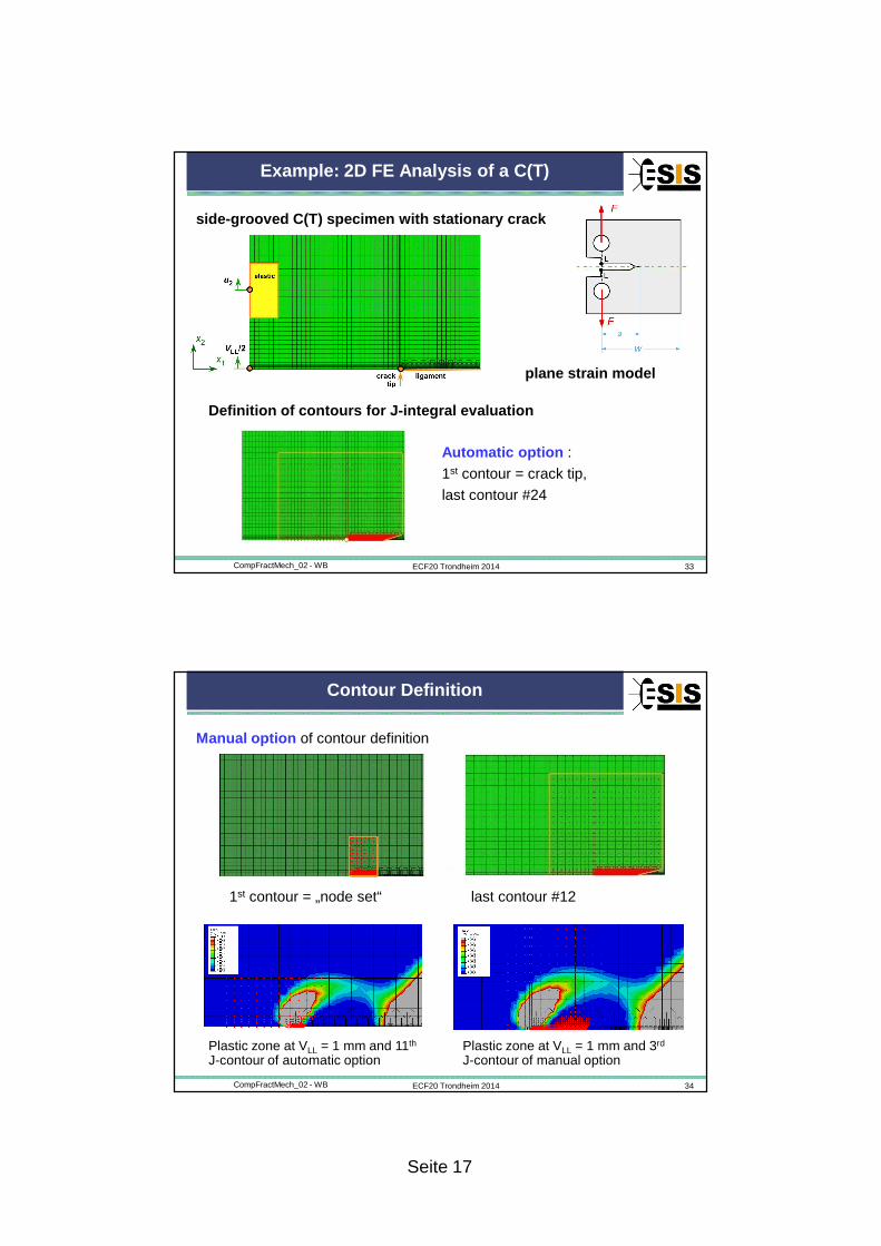
Example: 2D FE Analysis of a C(T)

side-grooved C(T) specimen with stationary crack

plane strain model

Definition of contours for J-integral evaluation

Automatic option :

1st contour = crack tip,

last contour #24


Contour Definition

1st contour = „node set“

Manual option of contour definition

last contour #12

Plastic zone at VLL = 1 mm and 11th

J-contour of automatic option Plastic zone at VLL = 1 mm and 3rd

J-contour of manual option

Seite 18


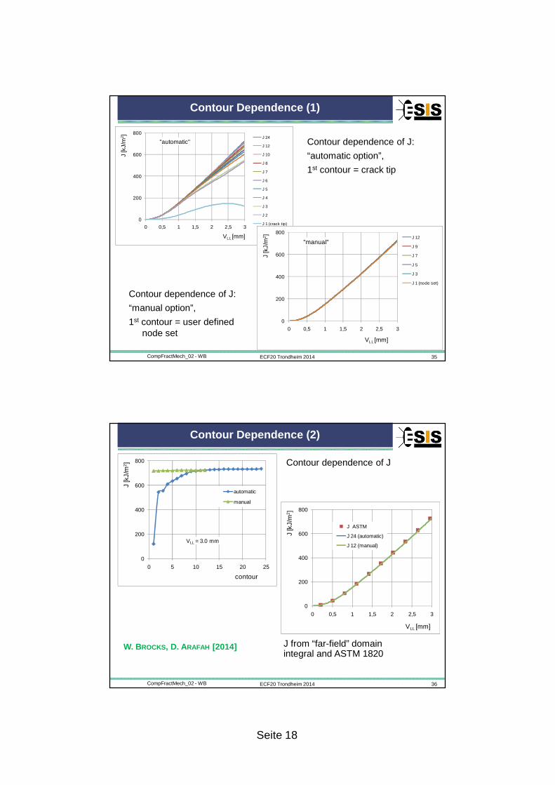
Contour Dependence (1)

Contour dependence of J:

“automatic option”,

1st contour = crack tip

Contour dependence of J:

“manual option”,

1st contour = user defined node set

0

200

400

600

800

0 0,5 1 1,5 2 2,5 3

J [k

J/m

2 ]

VLL [mm]

"automatic"J 24

J 12

J 10

J 8

J 7

J 6

J 5

J 4

J 3

J 2

J 1 (crack tip)

0

200

400

600

800

0 0,5 1 1,5 2 2,5 3

J [k

J/m

2 ]

VLL [mm]

"manual"J 12

J 9

J 7

J 5

J 3

J 1 (node set)


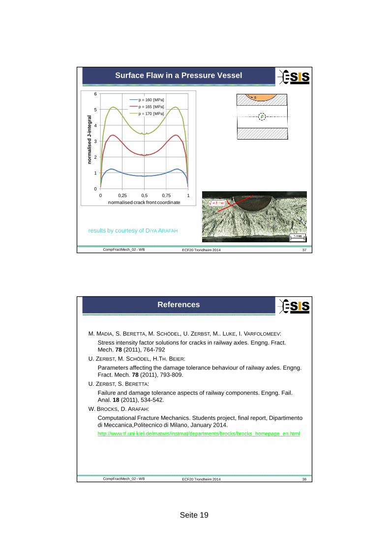
Contour Dependence (2)

W. BROCKS, D. ARAFAH [2014]

0

200

400

600

800

0 5 10 15 20 25

J[k

J/m

2]

contour

VLL = 3.0 mm

automatic

manual

J from “far-field” domain integral and ASTM 1820

0

200

400

600

800

0 0,5 1 1,5 2 2,5 3

J [k

J/m

2]

VLL [mm]

J_ASTM

J 24 (automatic)

J 12 (manual)

Contour dependence of J

Seite 19


Surface Flaw in a Pressure Vessel

0

1

2

3

4

5

6

0 0,25 0,5 0,75 1

norm

alis

ed J

-inte

gral

normalised crack front coordinate

p = 160 [MPa]

p = 165 [MPa]

p = 170 [MPa]

results by courtesy of DIYA ARAFAH


References

M. MADIA, S. BERETTA, M. SCHÖDEL, U. ZERBST, M.. LUKE, I. VARFOLOMEEV:

Stress intensity factor solutions for cracks in railway axles. Engng. Fract. Mech. 78 (2011), 764-792

U. ZERBST, M. SCHÖDEL, H.TH. BEIER:

Parameters affecting the damage tolerance behaviour of railway axles. Engng. Fract. Mech. 78 (2011), 793-809.

U. ZERBST, S. BERETTA:

Failure and damage tolerance aspects of railway components. Engng. Fail. Anal. 18 (2011), 534-542.

W. BROCKS, D. ARAFAH:

Computational Fracture Mechanics. Students project, final report, Dipartimentodi Meccanica,Politecnico di Milano, January 2014.http://www.tf.uni-kiel.de/matwis/instmat/departments/brocks/brocks_homepage_en.html

Seite 1


Part III: The Cohesive Model

Wolfgang Brocks


(1) Background - Fundamentals(2) The Traction-Separation Law(3) Examples, Applications(4) Cohesive Elements in ABAQUS


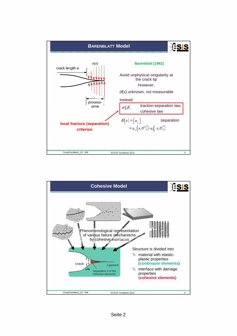
Simulation of Crack Extension

� Morphological

� Node release + fracture mechanics criterion (R-curve)

� no splitting of dissipation into global plasticity and local separation

� Cohesive surface

� Interface elements with traction-separation law responsible for local separation

� Continuum damage mechanics

� Unified constitutive equations for deformation and damage, e.g. porous metal plasticity

Seite 2


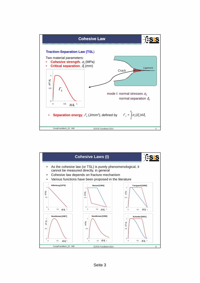
BARENBLATT Model

Barenblatt [1962]

Avoid unphysical singularity at the crack tip

However:

σ(x) unknown, not measurable

traction-separation law,

cohesive law

( )( ) ( ),0 ,0

y

y y

x u

u x u x

δ =

= −+ −

instead:

( )σ δ

separationlocal fracture (separation)

criterion


Cohesive Model

Structure is divided into

� material with elastic-plastic properties (continuum elements )

� interface with damage properties (cohesive elements )

∆a

crack Ligament

Separation δ of the cohesive elements

Phenomenological representation of various failure mechanisms

by cohesive interfacesOverview

Seite 3


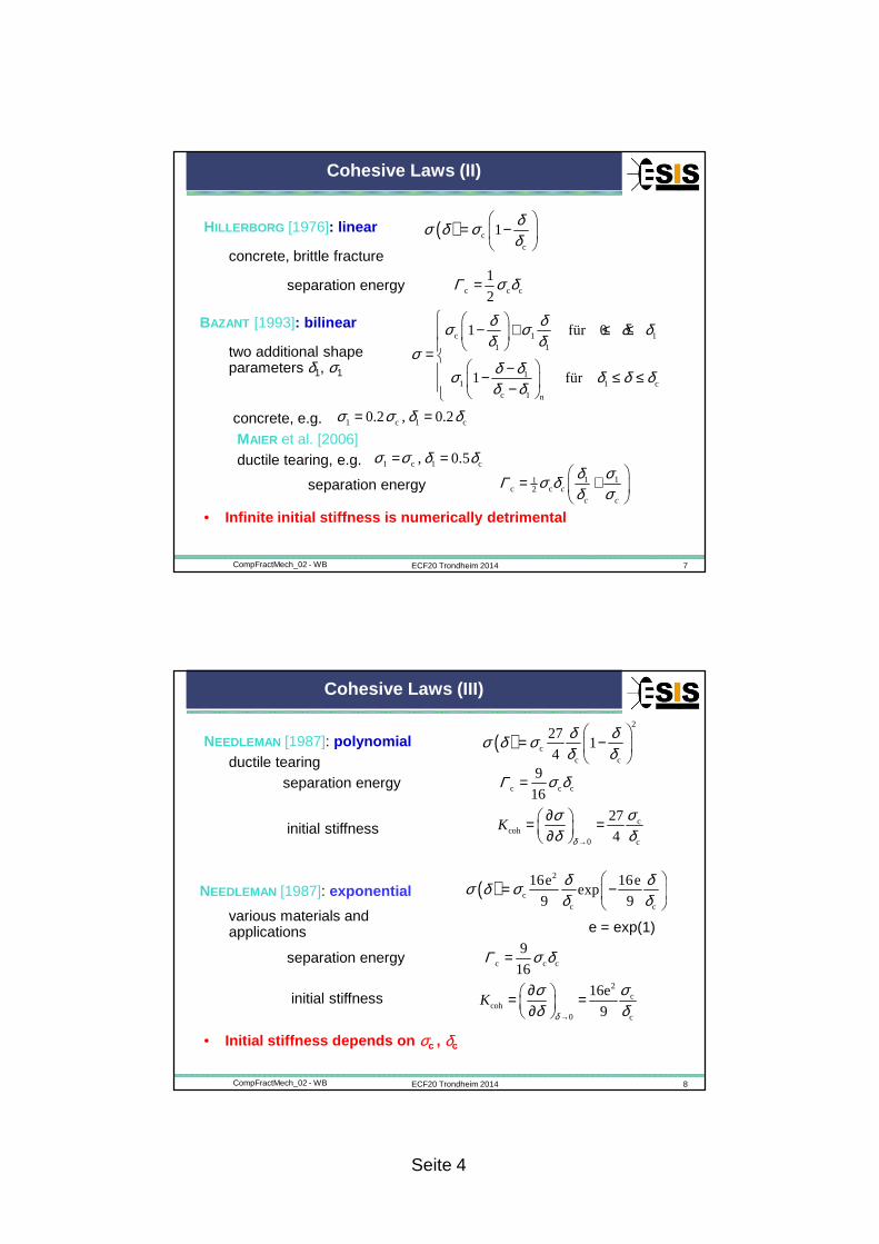
Cohesive LawCohesive Law

CrackLigament

Two material parameters:• Cohesive strength , σc (MPa)• Critical separation , δc (mm)

δ

Γ σ δ δ= ∫c

c n n n0

( )d• Separation energy , Γc (J/mm2), defined by

mode I: normal stresses σn

normal separation δn

Traction-Separation Law (TSL )

0

0,5

1

0 0,5 1

σ/ σ

c

δ /δc

Γc


Cohesive Laws (I)

• As the cohesive law (or TSL) is purely phenomenological, it cannot be measured directly, in general

• Cohesive law depends on fracture mechanism• Various functions have been proposed in the literature

0

0,5

1

0 0,5 1

σ/ σ

c

δ /δc

Hillerborg [1976]

0

0,5

1

0 0,5 1

σ/ σ

c

δ /δc

Bazant [1993]

0

0,5

1

0 0,5 1

σ/ σ

c

δ /δc

Tvergaard [1992]

0

0,5

1

0 0,5 1

σ / σ

c

δ /δc

Needleman [1987]

0

0,5

1

0 0,5 1

σ/ σ

c

δ /δc

Needleman [1990]

0

0,5

1

0 0,5 1

σ/ σ

c

δ /δc

Scheider [2001]

Seite 4


Cohesive Laws (II)

• Infinite initial stiffness is numerically detriment al

( ) cc

1δσ δ σδ

= −

c c c

1

2Γ σ δ=

HILLERBORG [1976]: linear

concrete, brittle fracture

separation energy

1 c 1 c, 0.5σ σ δ δ= =ductile tearing, e.g.

c 1 11 1

11 1 c

c 1 n

1 für 0

1 für

δ δσ σ δ δδ δ

σδ δσ δ δ δδ δ

− + ≤ ≤

= − − ≤ ≤ −

two additional shape parameters δ1, σ1

BAZANT [1993]: bilinear

1 c 1 c0.2 , 0.2σ σ δ δ= =concrete, e.g.MAIER et al. [2006]

1 11c c2 c

c c

δ σΓ σ δδ σ

= +

separation energy


Cohesive Laws (III)

• Initial stiffness depends on σc , δc

ductile tearing( )

2

cc c

271

4

δ δσ δ σδ δ

= −

NEEDLEMAN [1987]: polynomial

c c c

9

16Γ σ δ=separation energy

ccoh

0 c

27

4δ

σσδ δ→

∂ = = ∂ Kinitial stiffness

NEEDLEMAN [1987]: exponential ( )2

cc c

16e 16eexp

9 9

δ δσ δ σδ δ

= −

e = exp(1)various materials and applications

c c c

9

16Γ σ δ=separation energy

2c

coh0 c

16e

9δ

σσδ δ→

∂ = = ∂ Kinitial stiffness

Seite 5


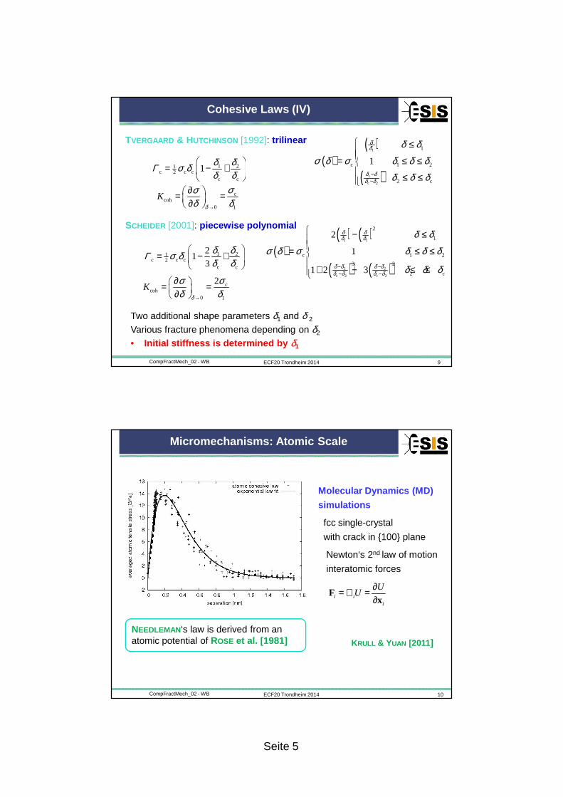
Cohesive Laws (IV)

Two additional shape parameters δ1 and δ 2

Various fracture phenomena depending on δ2

• Initial stiffness is determined by δ1

TVERGAARD & HUTCHINSON [1992]: trilinear

( )( )

( )

1

c

c 2

1

c 1 2

2 c

1

δδ

δ δδ δ

δ δ

σ δ σ δ δ δ

δ δ δ−−

≤= ≤ ≤ ≤ ≤

1 21c c c2

c c

1δ δΓ σ δδ δ

= − +

ccoh

0 1δ

σσδ δ→

∂ = = ∂ K

( )( ) ( )

( ) ( )

1 1

2 2

c 2 c 2

2

1

c 1 2

3 2

2 c

2

1

1 2 3

δ δδ δ

δ δ δ δδ δ δ δ

δ δ

σ δ σ δ δ δ

δ δ δ− −− −

− ≤= ≤ ≤

+ − ≤ ≤

1 21c c c2

c c

21

3

δ δΓ σ δδ δ

= − +

SCHEIDER [2001]: piecewise polynomial

ccoh

0 1

2

δ

σσδ δ→

∂ = = ∂ K


Micromechanisms: Atomic Scale

Molecular Dynamics (MD)

simulations

fcc single-crystal

with crack in {100} plane

KRULL & YUAN [2011]

Newton‘s 2nd law of motion

interatomic forces

i ii

UU

∂= =∂

Fx

∇

NEEDLEMAN ‘s law is derived from an atomic potential of ROSE et al. [1981]

Seite 6


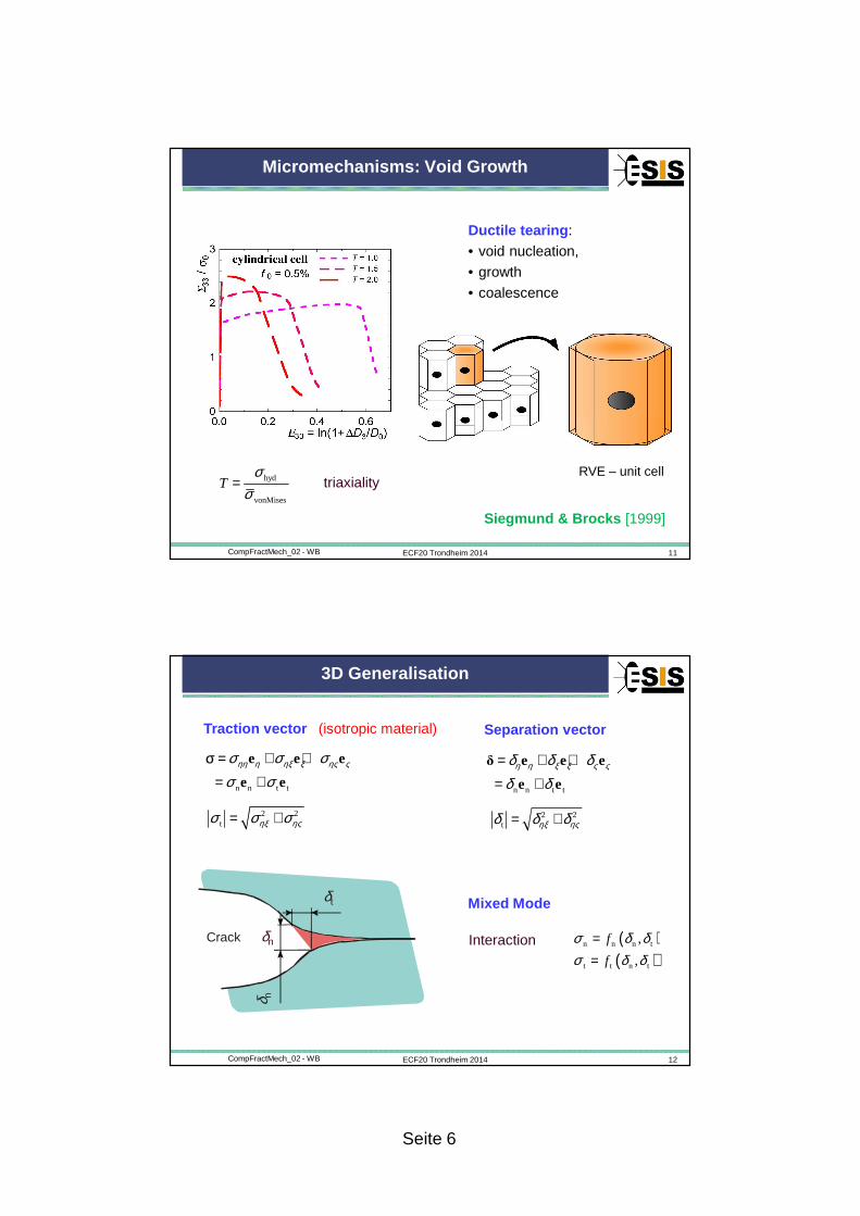
Micromechanisms: Void Growth

Ductile tearing :

• void nucleation,

• growth

• coalescence

RVE – unit cellhyd

vonMises

σσ

=T triaxiality

Siegmund & Brocks [1999]


3D Generalisation

Traction vector

n n t t

ηη η ηξ ξ ης ςσ σ σσ σ

= + +

= +

e e e

e e

σ

(isotropic material)

2 2t ηξ ηςσ σ σ= +

Separation vector

n n t t

η η ξ ξ ς ςδ δ δδ δ

= + +

= +

δ e e e

e e

2 2t ηξ ηςδ δ δ= +

Crack

δt

δ n

δn Interaction ( )( )

n n n t

t t n t

,

,

f

f

σ δ δσ δ δ

==

Mixed Mode

Seite 7


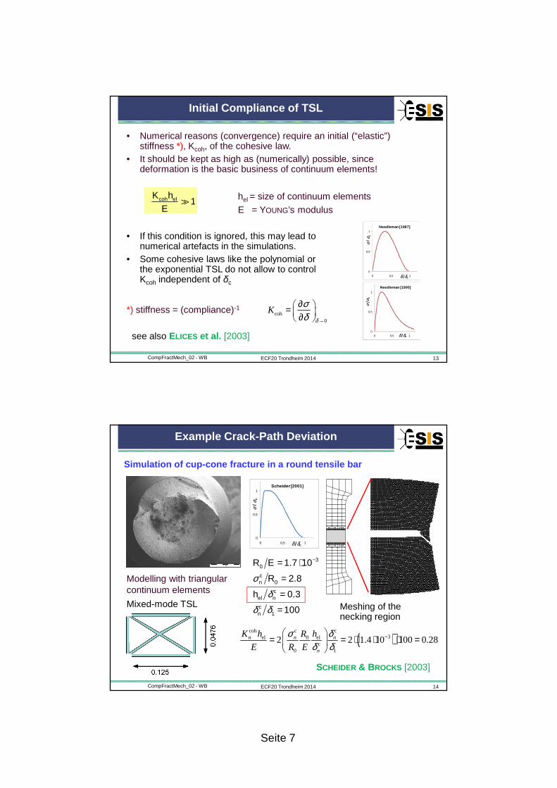
Initial Compliance of TSL

• Numerical reasons (convergence) require an initial (“elastic”) stiffness *), Kcoh, of the cohesive law.

• It should be kept as high as (numerically) possible, since deformation is the basic business of continuum elements!

• If this condition is ignored, this may lead to numerical artefacts in the simulations.

• Some cohesive laws like the polynomial or the exponential TSL do not allow to control Kcoh independent of δc

hel = size of continuum elements

E = YOUNG’s moduluscoh el 1

K hE

≫

*) stiffness = (compliance)-1coh

0δ

σδ →

∂ = ∂ K

0

0,5

1

0 0,5 1

σ/ σ

c

δ /δc

Needleman [1990]

0

0,5

1

0 0,5 1

σ / σ

c

δ /δc

Needleman [1987]

see also ELICES et al. [2003]


Example Crack-Path Deviation

Simulation of cup-cone fracture in a round tensile bar

Meshing of the necking region

SCHEIDER & BROCKS [2003]

Modelling with triangular continuum elements

Mixed-mode TSL

( )coh c c

3el 0 elc

0 1

2 2 1.4 10 100 0.28σ δ

δ δ−

= = ⋅ ⋅ ⋅ =

n n n

n

K h R h

E R E

0

0,5

1

0 0,5 1

σ/ σ

c

δ /δc

Scheider [2001]

30

c0

cel

c1

1.7 10

2.8

0.3

100

n

n

n

R E

R

h

σδ

δ δ

−= ⋅

=

=

=

Seite 8


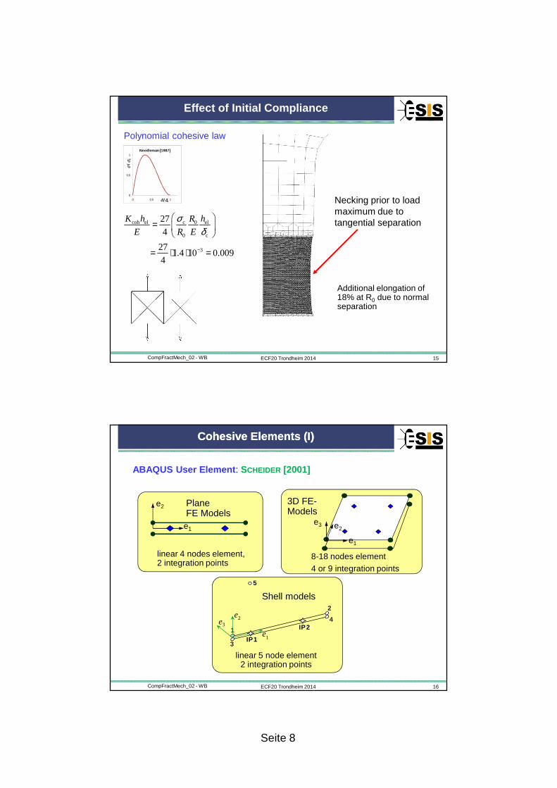
Effect of Initial Compliance

Additional elongation of 18% at R0 due to normal separation

Necking prior to load maximum due to tangential separation

Polynomial cohesive law

0

0,5

1

0 0,5 1

σ / σ

c

δ /δc

Needleman [1987]

coh el c 0 el

0 c

3

27

4

271.4 10 0.009

4

σδ

−

=

= ⋅ ⋅ =

K h R h

E R E


Cohesive Elements (I)Cohesive Elements (I)

Plane FE Models

e1

e2

linear 4 nodes element, 2 integration points

3D FE-Models

e1

e2e3

8-18 nodes element 4 or 9 integration points

1

2

3

4

IP1

IP2e1

e2e3

5

Shell models

linear 5 node element2 integration points

ABAQUS User Element : SCHEIDER [2001]

Seite 9


Cohesive Elements (II)

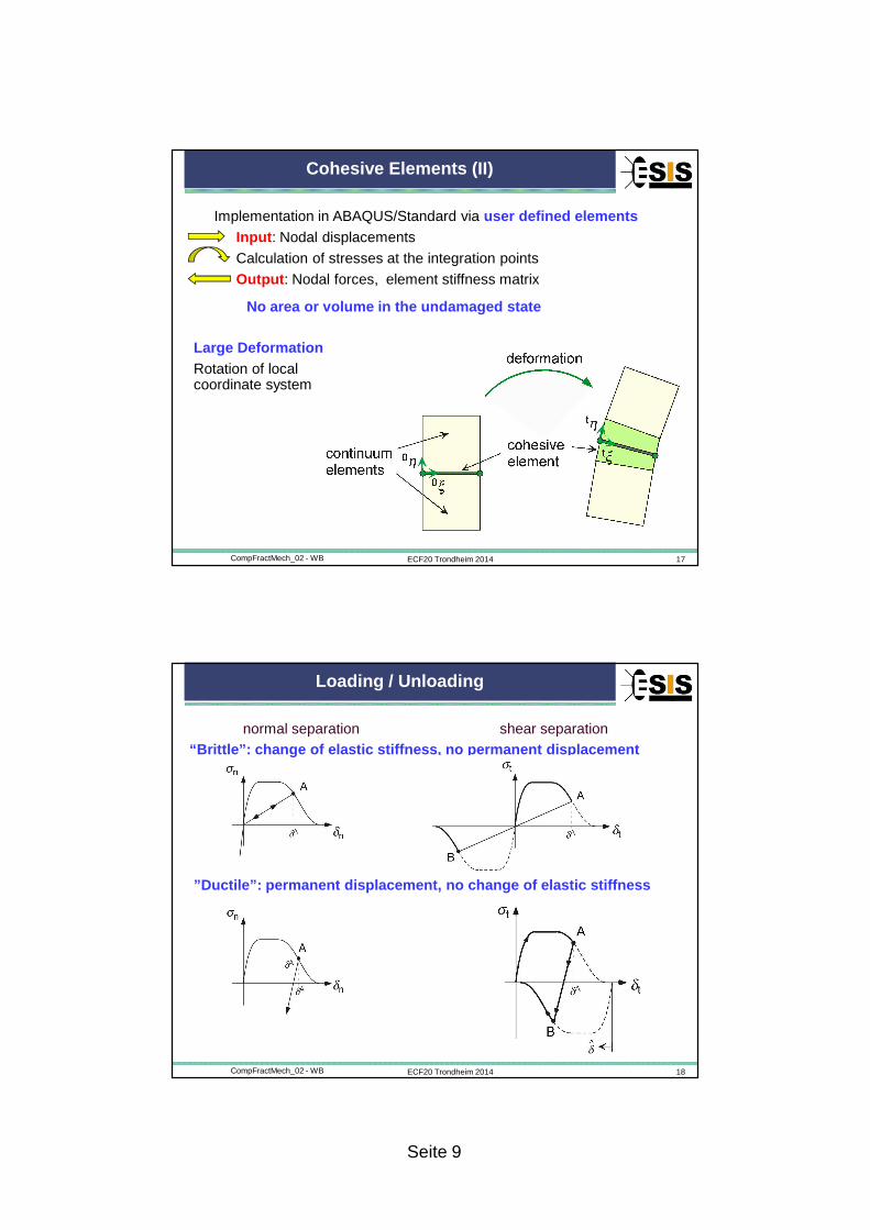
Implementation in ABAQUS/Standard via user defined elementsInput : Nodal displacements

Calculation of stresses at the integration points

Output : Nodal forces, element stiffness matrix

No area or volume in the undamaged state

Large DeformationRotation of local coordinate system


Loading / Unloading

“Brittle”: change of elastic stiffness, no permanen t displacementnormal separation shear separation

”Ductile”: permanent displacement, no change of ela stic stiffness

Seite 10


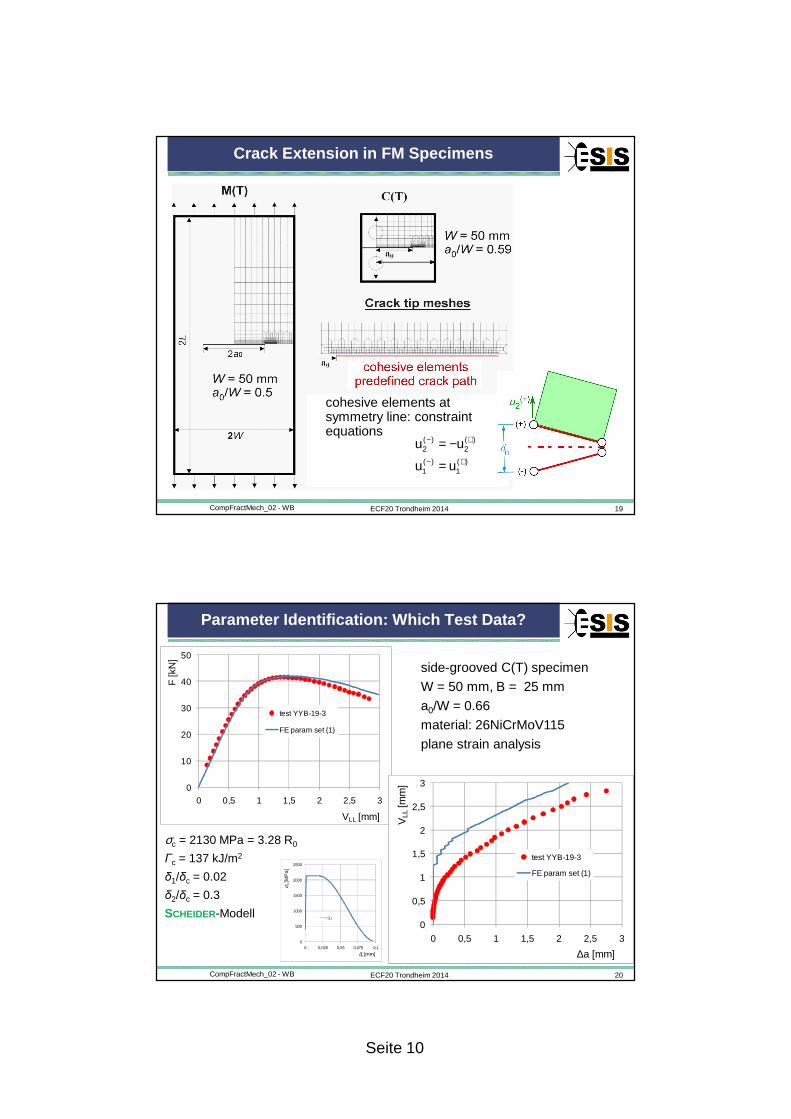
Crack Extension in FM Specimens

cohesive elements at symmetry line: constraint equations

( ) ( )2 2

( ) ( )1 1

u u

u u

− +

− +

= −

=


Parameter Identification: Which Test Data?

side-grooved C(T) specimen

W = 50 mm, B = 25 mm

a0/W = 0.66

material: 26NiCrMoV115

plane strain analysis

σc = 2130 MPa = 3.28 R0

Γc = 137 kJ/m2

δ1/δc = 0.02

δ2/δc = 0.3

SCHEIDER-Modell

0

10

20

30

40

50

0 0,5 1 1,5 2 2,5 3

F[k

N]

VLL [mm]

test YYB-19-3

FE param set (1)

0

0,5

1

1,5

2

2,5

3

0 0,5 1 1,5 2 2,5 3

VLL

[mm

]

∆a [mm]

test YYB-19-3

FE param set (1)

0

500

1000

1500

2000

2500

0 0,025 0,05 0,075 0,1

σ n[M

Pa]

δn [mm]

(1)

Seite 11


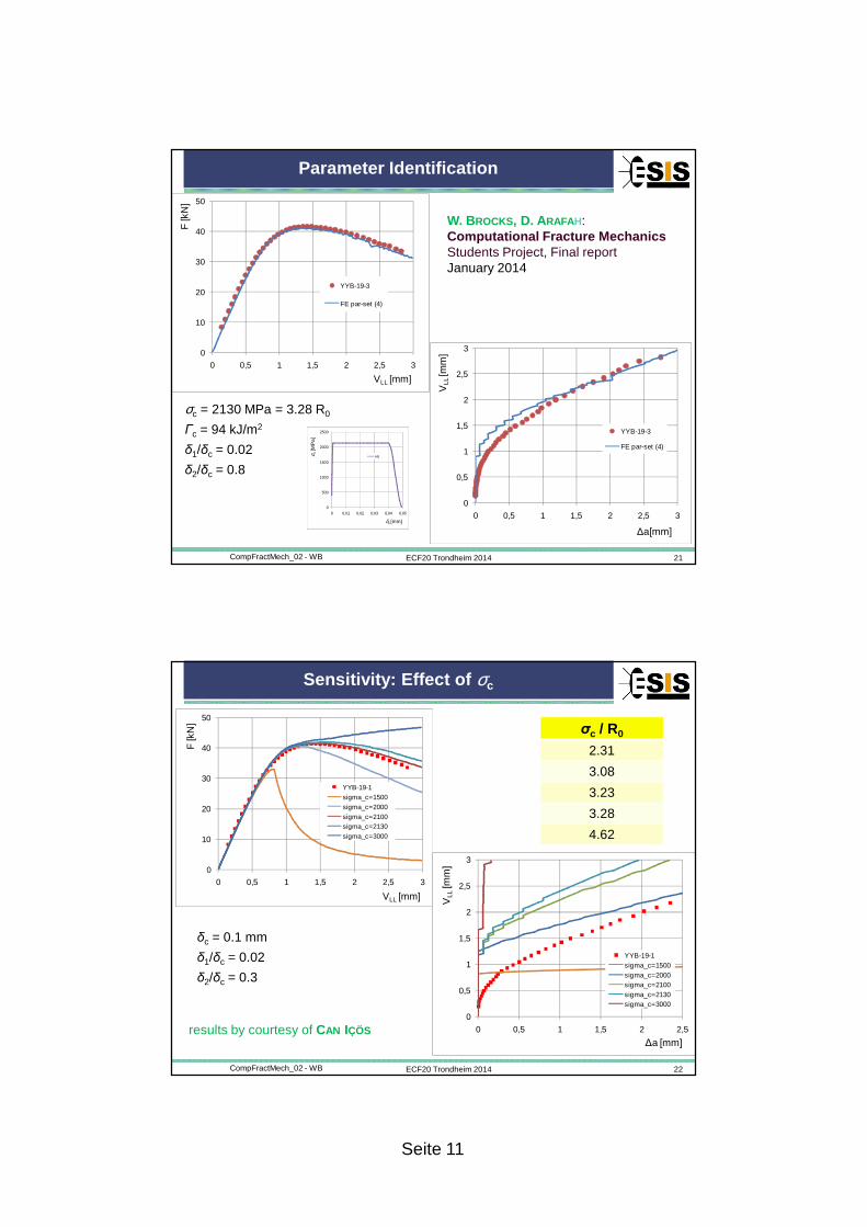
Parameter Identification

0

10

20

30

40

50

0 0,5 1 1,5 2 2,5 3

F[k

N]

VLL [mm]

YYB-19-3

FE par-set (4)

0

0,5

1

1,5

2

2,5

3

0 0,5 1 1,5 2 2,5 3

VLL

[mm

]

∆a[mm]

YYB-19-3

FE par-set (4)

σc = 2130 MPa = 3.28 R0

Γc = 94 kJ/m2

δ1/δc = 0.02

δ2/δc = 0.8

W. BROCKS, D. ARAFAH:Computational Fracture MechanicsStudents Project, Final reportJanuary 2014

0

500

1000

1500

2000

2500

0 0,01 0,02 0,03 0,04 0,05

σ n[M

Pa

]

δn [mm]

(4)


Sensitivity: Effect of σc

0

10

20

30

40

50

0 0,5 1 1,5 2 2,5 3

F[k

N]

VLL [mm]

YYB-19-1sigma_c=1500sigma_c=2000sigma_c=2100sigma_c=2130sigma_c=3000

0

0,5

1

1,5

2

2,5

3

0 0,5 1 1,5 2 2,5

VLL

[mm

]

∆a [mm]

YYB-19-1sigma_c=1500sigma_c=2000sigma_c=2100sigma_c=2130sigma_c=3000

δc = 0.1 mm

δ1/δc = 0.02

δ2/δc = 0.3

results by courtesy of CAN IÇÖS

σc / R0

2.31

3.08

3.23

3.28

4.62

Seite 12


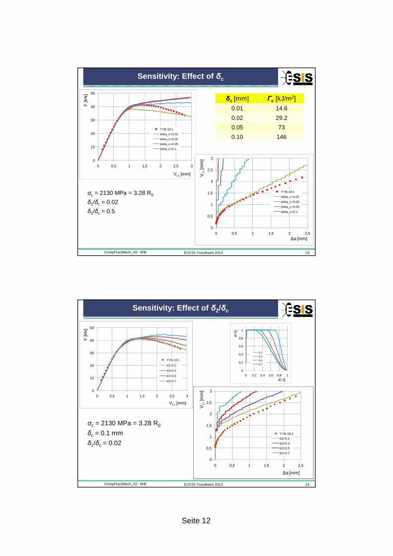
Sensitivity: Effect of δc

0

10

20

30

40

50

0 0,5 1 1,5 2 2,5 3

F[k

N]

VLL [mm]

YYB-19-1

delta_c=0.01

delta_c=0.02

delta_c=0.05

delta_c=0.1

0

0,5

1

1,5

2

2,5

3

0 0,5 1 1,5 2 2,5

VLL

[mm

]

∆a [mm]

YYB-19-1

delta_c=0.01

delta_c=0.02

delta_c=0.05

delta_c=0.1

σc = 2130 MPa = 3.28 R0

δ1/δc = 0.02

δ2/δc = 0.5

δc [mm] Γc [kJ/m2]

0.01 14.6

0.02 29.2

0.05 73

0.10 146


Sensitivity: Effect of δ2/δc

0

10

20

30

40

50

0 0,5 1 1,5 2 2,5 3

F[k

N]

VLL [mm]

YYB-19-1

d2=0.2

d2=0.3

d2=0.5

d2=0.7

0

0,5

1

1,5

2

2,5

3

0 0,5 1 1,5 2 2,5

VL

L[m

m]

∆a [mm]

YYB-19-1

d2=0.2

d2=0.3

d2=0.5

d2=0.7

σc = 2130 MPa = 3.28 R0

δc = 0.1 mm

δ1/δc = 0.02

0

0,2

0,4

0,6

0,8

1

0 0,2 0,4 0,6 0,8 1

σ/σ

c

δ / δc

0,2

0,3

0,5

0,7

Seite 13


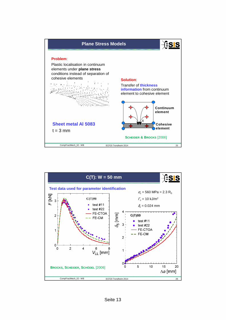
Plane Stress Models

Continuumelement

Cohesiveelement

t

Solution :

Transfer of thickness information from continuum element to cohesive element

Problem :

Plastic localisation in continuum elements under plane stressconditions instead of separation of cohesive elements

Sheet metal Al 5083t = 3 mm

SCHEIDER & BROCKS [2006]


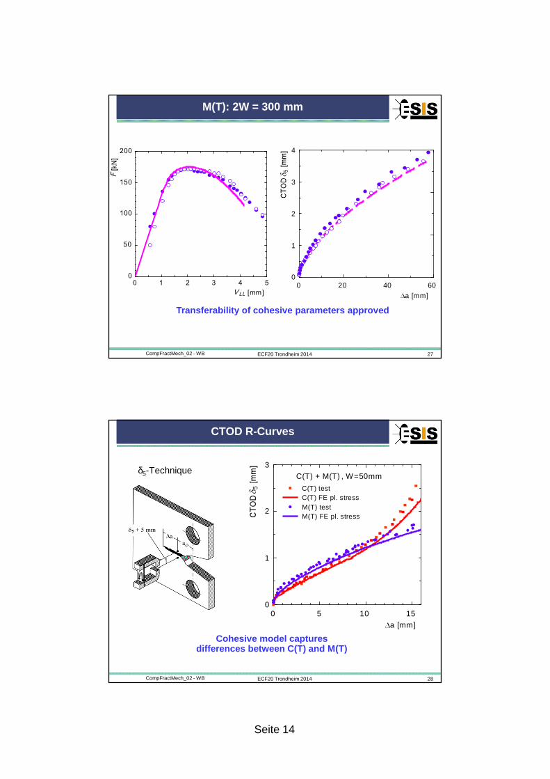
C(T): W = 50 mm

Test data used for parameter identificationσc = 560 MPa = 2.3 R0

Γc = 10 kJ/m2

δc = 0.024 mm

BROCKS, SCHEIDER, SCHÖDEL [2006]

Seite 14


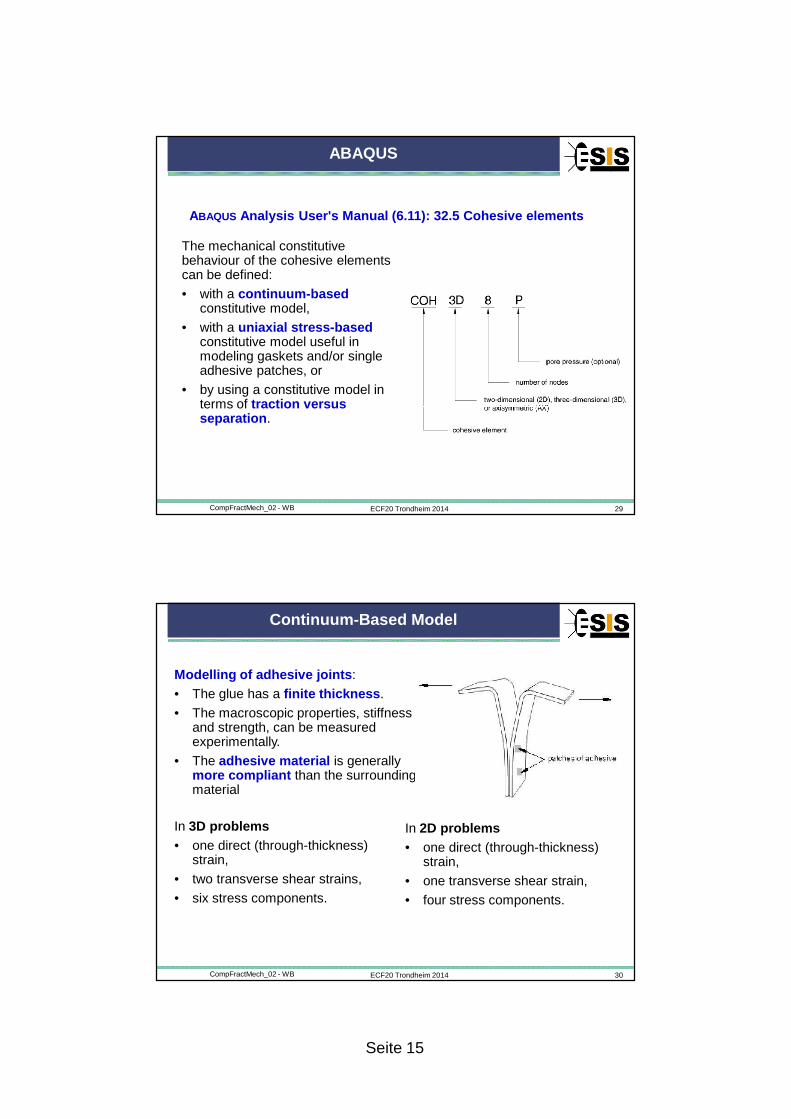
M(T): 2W = 300 mm

0 1 2 3 4 50

50

100

150

200

V LL [mm]0 20 40 60

0

1

2

3

4

a [mm]

Transferability of cohesive parameters approved


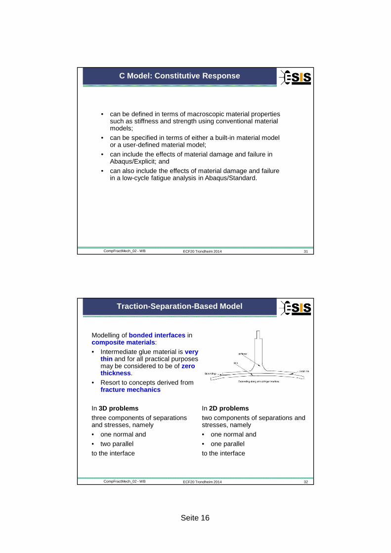
CTOD R-Curves

δ5-Technique

0 5 10 150

1

2

3

a [mm]

C(T) + M(T) , W=50mm

C(T) testC(T) FE pl. stressM(T) testM(T) FE pl. stress

Cohesive model captures differences between C(T) and M(T)

Seite 15


ABAQUS

ABAQUS Analysis User's Manual (6.11): 32.5 Cohesive elemen ts

The mechanical constitutive behaviour of the cohesive elements can be defined:

• with a continuum-basedconstitutive model,

• with a uniaxial stress-basedconstitutive model useful in modeling gaskets and/or single adhesive patches, or

• by using a constitutive model in terms of traction versus separation .


Continuum-Based Model

Modelling of adhesive joints :

• The glue has a finite thickness .

• The macroscopic properties, stiffness and strength, can be measured experimentally.

• The adhesive material is generally more compliant than the surrounding material

In 3D problems• one direct (through-thickness)

strain,

• two transverse shear strains,

• six stress components.

In 2D problems• one direct (through-thickness)

strain,

• one transverse shear strain,

• four stress components.

Seite 16


C Model: Constitutive Response

• can be defined in terms of macroscopic material properties such as stiffness and strength using conventional material models;

• can be specified in terms of either a built-in material model or a user-defined material model;

• can include the effects of material damage and failure in Abaqus/Explicit; and

• can also include the effects of material damage and failure in a low-cycle fatigue analysis in Abaqus/Standard.


Traction-Separation-Based Model

Modelling of bonded interfaces in composite materials :

• Intermediate glue material is very thin and for all practical purposes may be considered to be of zero thickness .

• Resort to concepts derived from fracture mechanics

In 3D problemsthree components of separations and stresses, namely

• one normal and

• two parallel

to the interface

In 2D problemstwo components of separations and stresses, namely

• one normal and

• one parallel

to the interface

Seite 17


TS Model: Elastic

The traction-separation model assumes

• initially linear elastic behaviour relating the nominal stresses to the nominal strains across the interface,

• followed by the initiation and evolution of damage .

• The nominal stresses are the force components divided by the original area , while the nominal strains are the separationsdivided by the original thickness at each integration point.

• The default value of the original constitutive thickness is 1.0, which ensures that the nominal strain is equal to the separation.

• The constitutive thickness is usually different from the geometric thickness (which is typically close or equal to zero).

”fully coupled behaviour“


Initial Compliance

There is no coupling between normal and shear components in HOOKE’s law. Stress and strain tensor are coaxial.

0 0

0 0

0 0

nn

tt

ss

K

K

K

=

t

normal separation:coh

0

nnn nn n n n n

KK K

hσ ε δ δ= = =

coh

eln

EK

h≫

The initial compliance 1/Kcoh of the cohesive element depends on the „choice“ of its “constitutive thickness” h0!

Requirement (see above)

that is0

elnn

hK E

h≫

Knn has no physical meaning as the “constitutive thickness” h0 has no geometrical one. Both possess some numerical significance, only.

Seite 18


TS Model: “Damage”

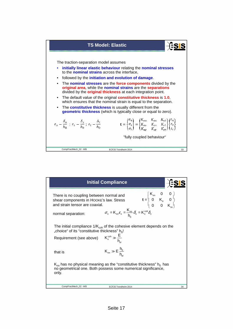
Damage :

• Once a damage initiation criterionis met, material damage can occur according to a user-defined damage evolution law.

• A scalar damage variable, D, represents the overall damage in the material and captures the combined effects of all the active mechanisms.

• Unloading subsequent to damage initiation is always assumed to occur linearly toward the origin of the traction-separation plane.

• Reloading subsequent to unloading also occurs along the same linear path until the softening envelope is reached.


TSLs

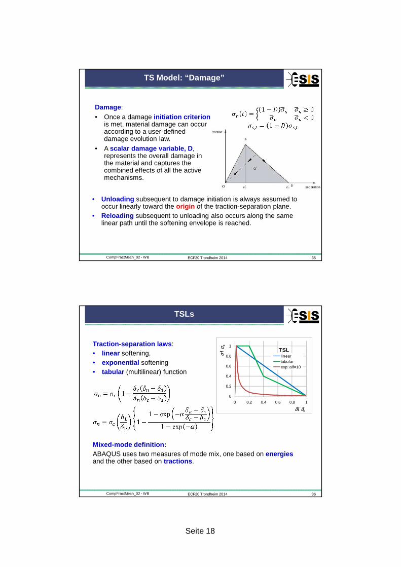
Mixed-mode definition :ABAQUS uses two measures of mode mix, one based on energiesand the other based on tractions .

Traction-separation laws : • linear softening, • exponential softening • tabular (multilinear) function

0

0,2

0,4

0,6

0,8

1

0 0,2 0,4 0,6 0,8 1

σ/ σ

c

δ / δc

TSLlineartabularexp: alf=10

Seite 19


”Damage“

0

0,2

0,4

0,6

0,8

1

0 0,2 0,4 0,6 0,8 1

D

δ / δc

"damage"lineartabularexp: alf=10

( ) ( ) 0coh

1 1n n n n

n n nn n

DK K

σ δ σ δ δδ δ

= − = −

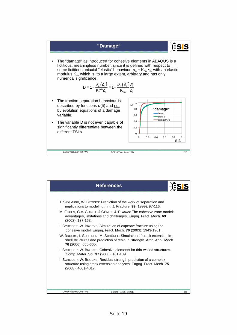
• The “damage“ as introduced for cohesive elements in ABAQUS is a fictitious, meaningless number, since it is defined with respect to some fictitious uniaxial ”elastic“ behaviour, σn = Knn εn, with an elastic modulus Knn which is, to a large extent, arbitrary and has only numerical significance.

• The traction-separation behaviour is described by functions σ(δ) and notby evolution equations of a damage variable.

• The variable D is not even capable of significantly differentiate between the different TSLs.


References

T. SIEGMUND, W. BROCKS: Prediction of the work of separation and implications to modeling . Int. J. Fracture 99 (1999), 97-116.

M. ELICES, G.V. GUINEA, J.GÓMEZ, J. PLANAS: The cohesive zone model: advantages, limitations and challenges. Engng. Fract. Mech. 69(2002), 137-163.

I. SCHEIDER, W. BROCKS: Simulation of cupcone fracture using the cohesive model. Engng. Fract. Mech. 70 (2003), 1943-1961.

W. BROCKS, I. SCHEIDER, M. SCHÖDEL: Simulation of crack extension in shell structures and prediction of residual strength. Arch. Appl. Mech. 76 (2006), 655-665.

I. SCHEIDER, W. BROCKS: Cohesive elements for thin-walled structures. Comp. Mater. Sci. 37 (2006), 101-109.

I. SCHEIDER, W. BROCKS: Residual strength prediction of a complex structure using crack extension analyses. Engng. Fract. Mech. 75(2008), 4001-4017.

Computational Fracture Mechanics - tf.uni-kiel.de · Computational Fracture Mechanics ......

Documents

Transcript of Computational Fracture Mechanics - tf.uni-kiel.de · Computational Fracture Mechanics ......