Computational Fluid Dynamics

Lecture 1

Author(s)

Barłomiej SzyjaF1/102

email: b.m.szyja@pwr.edu.pl

Wojciech LudwigC6/110

email: wojciech.ludwig@pwr.edu.pl

http://wludwig.pl

Literature

Presentation slides

Jaworski, Z. "Numeryczna mechanika płynów w inżynierii chemicznej i procesowej", Warszawa 2005

Szafran, R.G., „Modelowanie procesu suszenia w suszarce fontannowej”, Praca doktorska, Wrocław 2004

Ansys Fluent Help

Ansys on-line materials https://support.ansys.com/portal/site/AnsysCustomerPortal

http://www.bakker.org

Modern methods of chemical engineering processes design -CFD

Computer design

All existing and newly designed machines and technologies need continuous improvements:

increasing demands for product quality lowering the production costs to remain competitive tightening of security norms and environmental protection laws rapid changes in market demands

All these areas can greatly benefit from modern computers: numerical modeling of processes (e.g. CFD) CAD/CAM/CAE software databases Wide area computer networks computer control and automatization systems

Computer design

Software used in this area can be (roughly) divided into 3 groups: CAD (Computer Aided Design)

Software to draw/model/visualize 2D and 3D objects CAM (Computer Aided Manufacturing)

CAM systems are used for the production process. They make use of the projects created in CAD process and generate the code directly driving the machinery: metal lathe, milling machine, etc.

CAE (Computer Aided Engineering)The purpose of CAE systems is to help the engineers in their tasks, e.g. design, analysis or computations. This group comprises of process engineering software, "flowsheet modelling environments": Aspen Plus, CHEMCAD, HYSYS, ChemSep, specialized driers software: dryPAK, computational fluid dynamics software: CFX, FLUENT, FLOW3D etc.

Fluid mechanics

fluid statics Describes behavior of fluids in equilibrium state. Deals with the conditions where respective fluid elements are in constant position with respect to each other and container. Viscosity of fluid is neglected. It is considered a part of fluid mechanics.

fluid kinematicsInvestigation is focused on velocity fields of fluid in motion, however without taking into account the forces present in the system.

fluid dynamicsDeals with the forces present due to the motion of fluid in connection with the velocity fields of the fluid.

Fluid mechanics

Mechanics of the ideal fluidideal fluid does not have viscosity, its properties depend only on the density and pressure, it transfers only normal stresses

Mechanics of a real fluidreal fluid is characterized also by viscosity, and therefore transferring also shear stresses

Fluid mechanics

Experimental fluid mechanicsThe physical observations and measurements are done during the flow. Based on the results the physical and mathematical models are made.

Theoretical fluid mechanicsThe physical and mathematical models are made allowing to solve the formulas analytically. This is usually limited to simple flow problems.

Numerical fluid mechanicsUtilizes numerical (non-analytical) methods to solve flow problems.

Computational Fluid Dynamics

Computational fluid dynamics (CFD) is the science of predicting fluid flow, heat transfer, mass transfer, chemical reactions, and related phenomena by solving the mathematical equations, which govern these processes using a numerical method.

The result of CFD analyses is relevant engineering data used in:

Conceptual studies of new designs.

Detailed product development.

Troubleshooting.

Redesign.

CFD analysis complements testing and experimentation, reduces the total effort required in the laboratory.

Computational Fluid Dynamics

Analysis begins with a mathematical model of a physical problem.

Conservation of matter, momentum, and energy must be satisfied throughout the region of interest.

Fluid properties are modeled empirically.

Simplifying assumptions are made in order to make the problem tractable (e.g., steady-state, incompressible, inviscid, two-dimensional).

Provide appropriate initial and boundary conditions for the problem.

Computational Fluid Dynamics

CFD applies numerical methods (called discretization) to develop approximations of the governing equations of fluid mechanics in the fluid region of interest.

• Governing differential equations: algebraic.

• The collection of cells is called the grid or mesh.

• The set of algebraic equations are solved numerically (on a computer) for the flow field variables at each node or cell.

• System of equations are solved simultaneously to provide solution.

The solution is post-processed to extract quantities of interest (e.g. lift, drag, torque, heat transfer, separation, pressure loss, etc.).

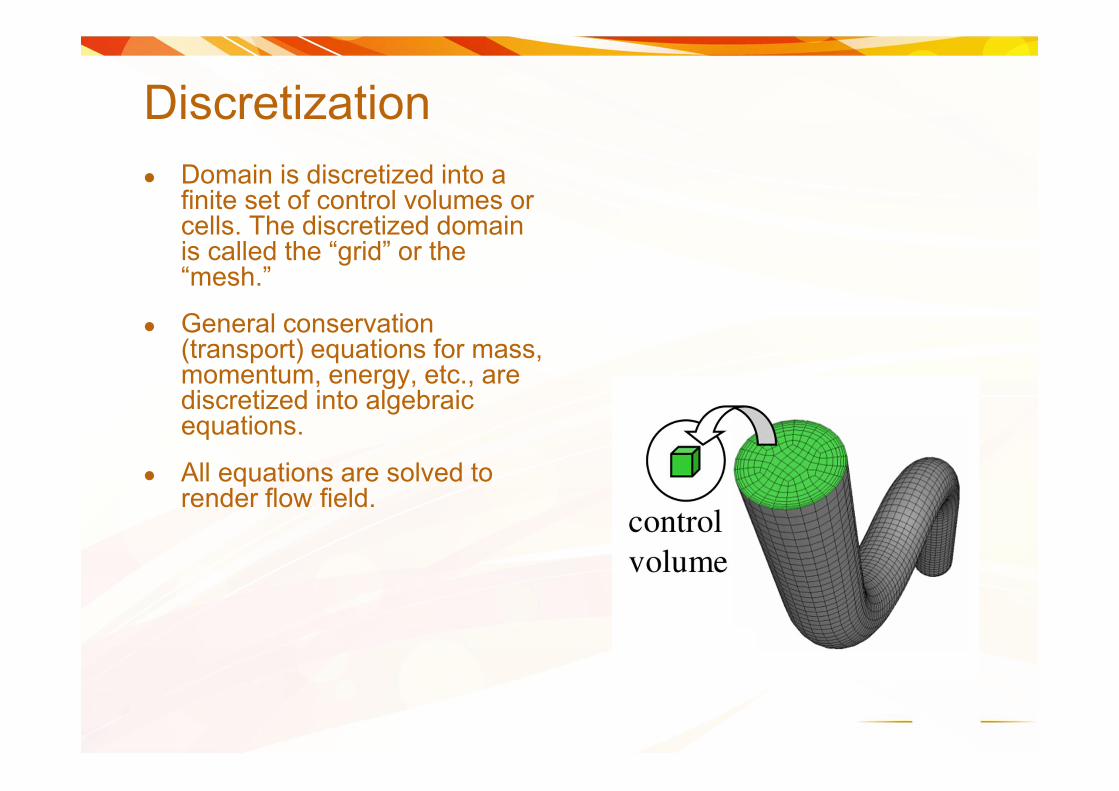
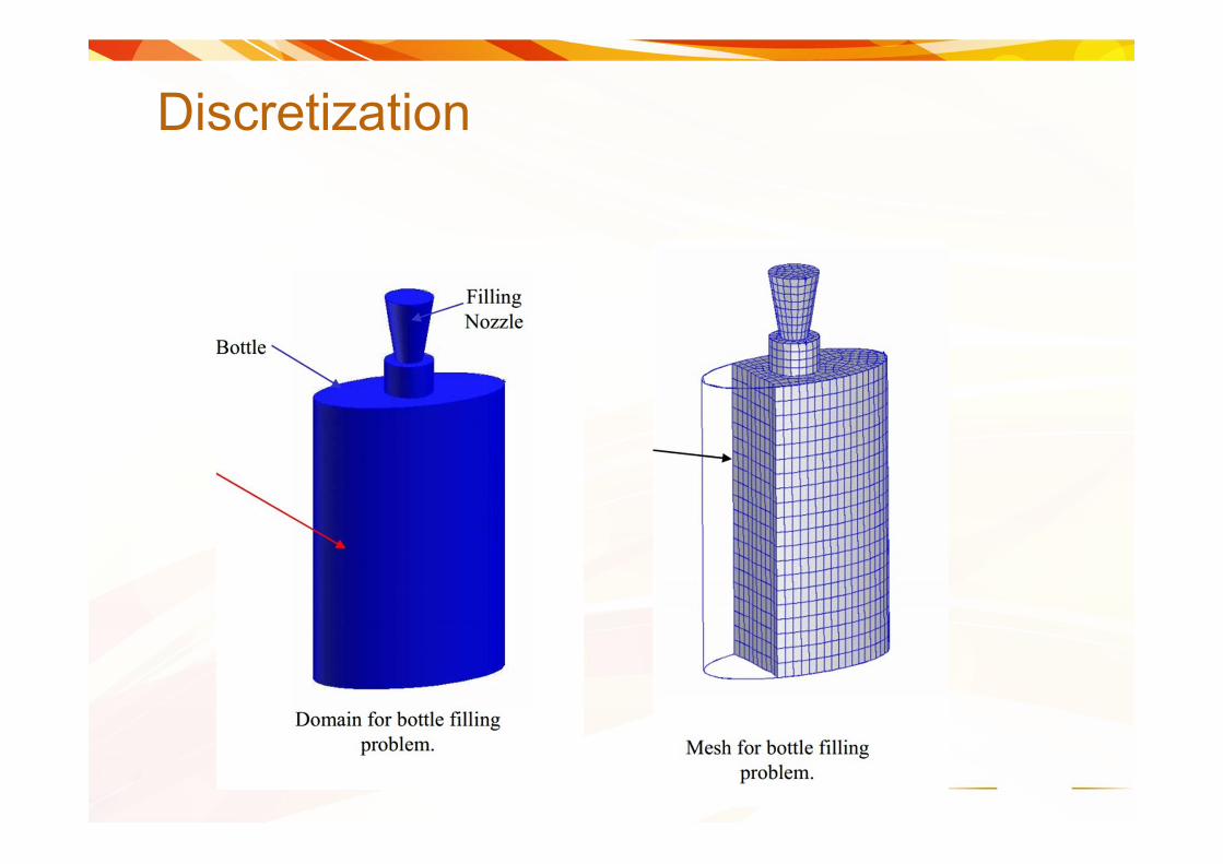
Discretization

Domain is discretized into a finite set of control volumes or cells. The discretized domain is called the “grid” or the “mesh.”

General conservation (transport) equations for mass, momentum, energy, etc., are discretized into algebraic equations.

All equations are solved to render flow field.

Discretization

Extensive quantities

Extensive quantities can be transported and summed in the finite area.

Substantial extensive quantities are related to the grains of substance (mater). The partition of the material area into subareas requires analogous partition of extensive quantities. These quantities include kinetic energy, mass and number of the component.

Non-substantial extensive quantities include volume and electromagnetic energy.

Scalar extensive quantities include volume, total mass, mass of the i-th component, entropy, electric charge, etc.

Vector extensive quantities include unit energy flow and momentum.

Intensive quantities

Intensive quantities are correlated to extensive quantities, but have the character of a potential.

Contrary to extensive quantities, potential does not depend on the dimensions of the area, and partition of the area does not lead to change of the potential. They form field values. Driving forces of transport are expressed as gradients of intensive parameters.

Intensive quantities include pressure, chemical potential, temperature, voltage, etc.

Pseudo-intensive quantities can be expressed as the quotient of two extensive quantities - for example volume or mass.

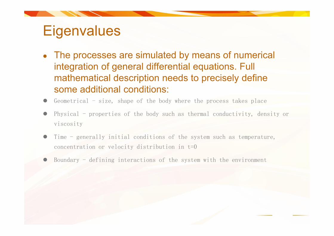
Eigenvalues

The processes are simulated by means of numerical integration of general differential equations. Full mathematical description needs to precisely define some additional conditions:

Geometrical - size, shape of the body where the process takes place

Physical - properties of the body such as thermal conductivity, density or

viscosity

Time - generally initial conditions of the system such as temperature,

concentration or velocity distribution in t=0

Boundary - defining interactions of the system with the environment

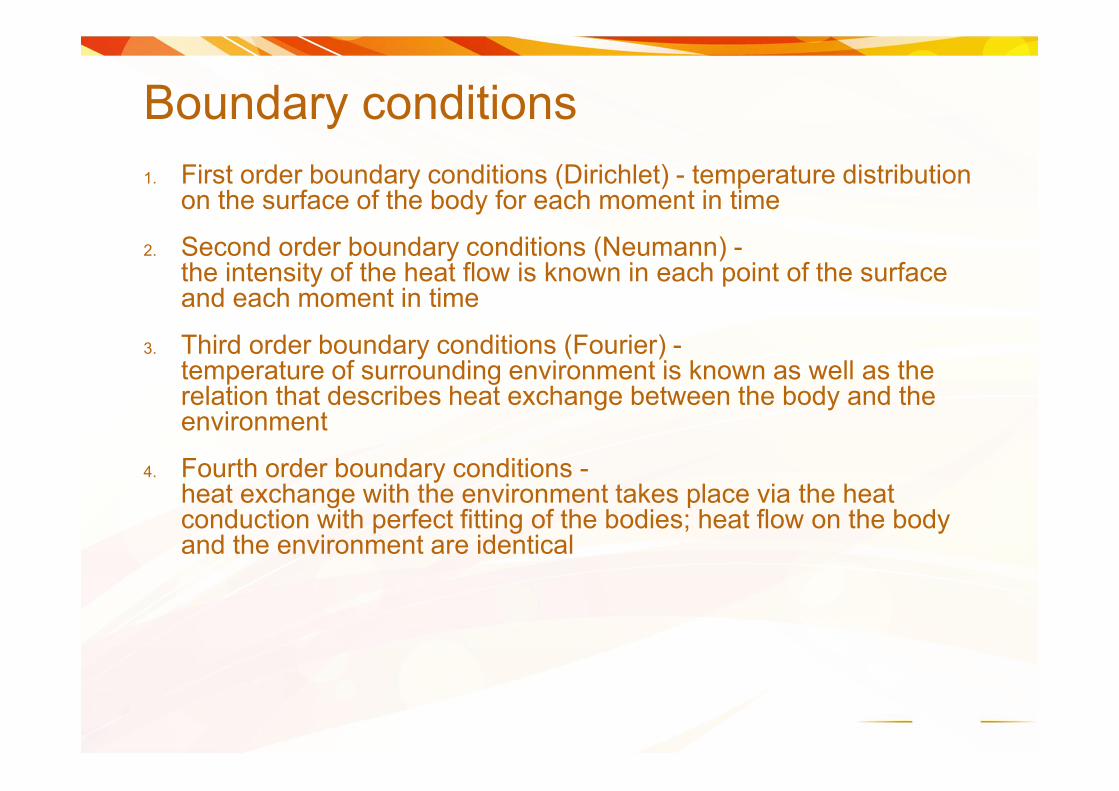
Boundary conditions

1. First order boundary conditions (Dirichlet) - temperature distribution on the surface of the body for each moment in time

2. Second order boundary conditions (Neumann) -the intensity of the heat flow is known in each point of the surface and each moment in time

3. Third order boundary conditions (Fourier) -temperature of surrounding environment is known as well as the relation that describes heat exchange between the body and the environment

4. Fourth order boundary conditions -heat exchange with the environment takes place via the heat conduction with perfect fitting of the bodies; heat flow on the body and the environment are identical

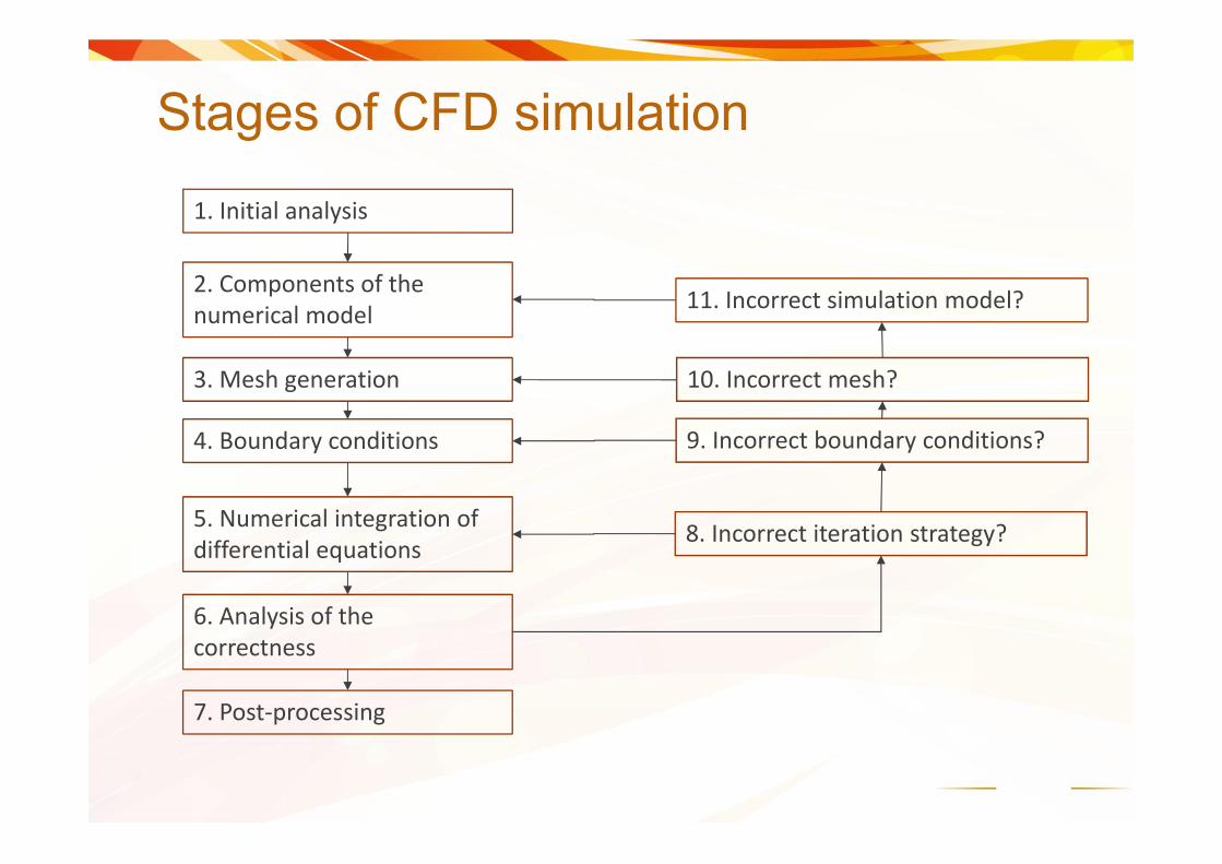
Stages of CFD simulation

1. Initial analysis

2. Components of the numerical model

3. Mesh generation

4. Boundary conditions

5. Numerical integration of differential equations

6. Analysis of the correctness

7. Post-processing

8. Incorrect iteration strategy?

9. Incorrect boundary conditions?

10. Incorrect mesh?

11. Incorrect simulation model?

Advantages of CFD

Relatively low cost. Using physical experiments and tests to get essential

engineering data for design can be expensive.

CFD simulations are relatively inexpensive, and costs are likely to decrease as computers become more powerful.

Speed. CFD simulations can be executed in a short period of time.

Quick turnaround means engineering data can be introduced early in the design process.

Ability to simulate real conditions. Many flow and heat transfer processes can not be (easily)

tested, e.g. hypersonic flow.

CFD provides the ability to theoretically simulate any physical condition.

Advantages of CFD

Ability to simulate ideal conditions. CFD allows great control over the physical process, and

provides the ability to isolate specific phenomena for study.

Example: a heat transfer process can be idealized with adiabatic, constant heat flux, or constant temperature boundaries.

Comprehensive information. Experiments only permit data to be extracted at a limited

number of locations in the system (e.g. pressure and temperature probes, heat flux gauges, LDV, etc.).

CFD allows the analyst to examine a large number of locations in the region of interest, and yields a comprehensive set of flow parameters for examination.

Limitations of CFD

Physical models. CFD solutions rely upon physical models of real world

processes (e.g. turbulence, compressibility, chemistry, multiphase flow, etc.).

The CFD solutions can only be as accurate as the physical models on which they are based.

Numerical errors. Solving equations on a computer invariably introduces

numerical errors.

Round-off error: due to finite word size available on the computer. Round-off errors will always exist (though they can be small in most cases).

Truncation error: due to approximations in the numerical models. Truncation errors will go to zero as the grid is refined. Mesh refinement is one way to deal with truncation error.

Limitations of CFD

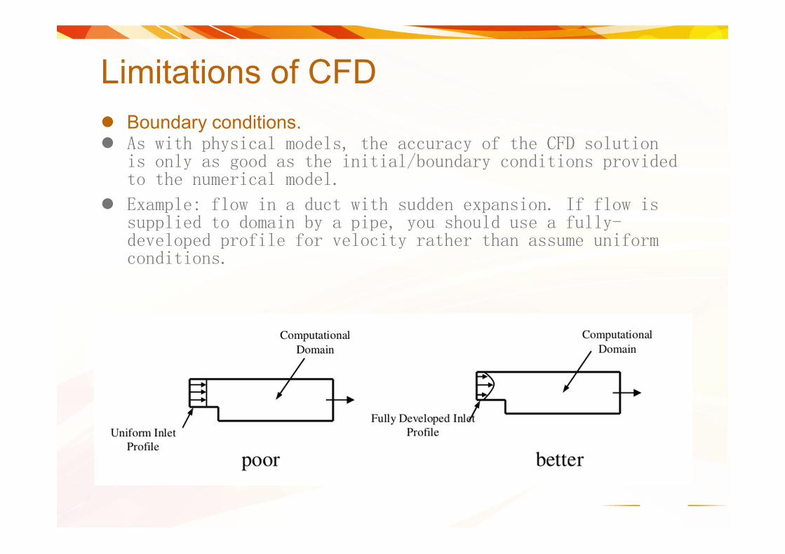
Boundary conditions. As with physical models, the accuracy of the CFD solution

is only as good as the initial/boundary conditions provided to the numerical model.

Example: flow in a duct with sudden expansion. If flow is supplied to domain by a pipe, you should use a fully-developed profile for velocity rather than assume uniform conditions.

Early work

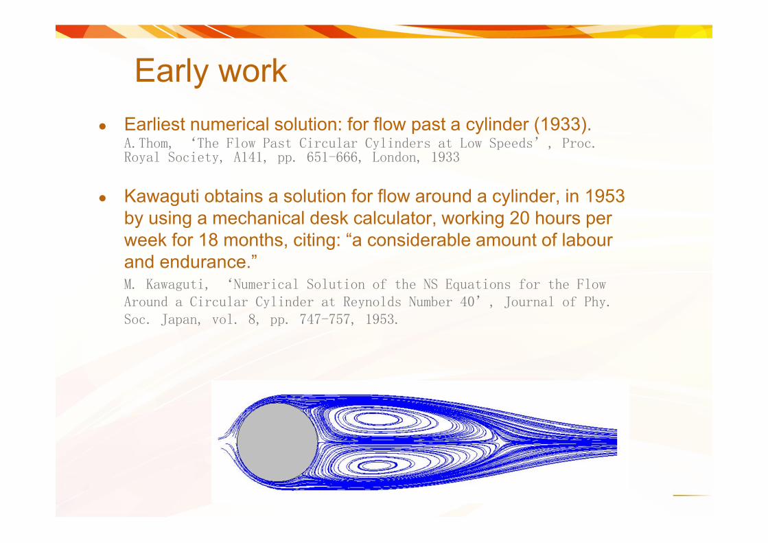
Earliest numerical solution: for flow past a cylinder (1933).A.Thom, ‘The Flow Past Circular Cylinders at Low Speeds’, Proc. Royal Society, A141, pp. 651-666, London, 1933

Kawaguti obtains a solution for flow around a cylinder, in 1953 by using a mechanical desk calculator, working 20 hours per week for 18 months, citing: “a considerable amount of labour and endurance.”M. Kawaguti, ‘Numerical Solution of the NS Equations for the Flow Around a Circular Cylinder at Reynolds Number 40’, Journal of Phy. Soc. Japan, vol. 8, pp. 747-757, 1953.

Development

Previously, CFD was performed using academic, research and in-house codes. When one wanted to perform a CFD calculation, one had to write a program.

This is the period during,which most commercial CFD codes originated that are available today:

Fluent (UK and US).

CFX (UK and Canada).

Fidap (US).

Polyflow (Belgium).

Phoenix (UK).

Star CD (UK).

Flow 3d (US).

ESI/CFDRC (US).

SCRYU (Japan).

and more, see www.cfdreview.com.

CFD in chemical engineering

Applications in chemical engineering include but are not limited to:

reactors and bioreactors, single- and multiphase

distillation, adsorption and absorption columns

mixers, settlers, cyclones

tanks and pipelines

heat exchangers

scrubbers

crystallizers

drying processes - pneumatic, fluidized, spouted bed dryers