Computational Complexity Theory - CSA
80
Computational Complexity Theory Lecture 1: Intro; Turing machines; Class P Department of Computer Science, Indian Institute of Science
Transcript of Computational Complexity Theory - CSA

Computational Complexity Theory
Lecture 1: Intro; Turing machines; Class P
Department of Computer Science, Indian Institute of Science
About the course
Computational complexity attempts to classify computational problems based on the amount of resources required by algorithms to solve them.

About the course
Computational complexity attempts to classify computational problems based on the amount of resources required by algorithms to solve them.
Computational problems come in various flavors:

About the course
Computational complexity attempts to classify computational problems based on the amount of resources required by algorithms to solve them.
Computational problems come in various flavors:
a. Decision problem
Example: Is vertex t reachable from vertex s in graph G?
(…output is YES/NO)

About the course
Computational complexity attempts to classify computational problems based on the amount of resources required by algorithms to solve them.
Computational problems come in various flavors:
a. Decision problem
b. Search problem
Example: Find a satisfying assignment of a Boolean
formula, if it exists.

About the course
Computational complexity attempts to classify computational problems based on the amount of resources required by algorithms to solve them.
Computational problems come in various flavors:
a. Decision problem
b. Search problem
c. Counting problem
Example: Find the number of cycles in a graph

About the course
Computational complexity attempts to classify computational problems based on the amount of resources required by algorithms to solve them.
Computational problems come in various flavors:
a. Decision problem
b. Search problem
c. Counting problem
d. Optimization problem
Example: Find a minimum size vertex cover in a graph

About the course
Computational complexity attempts to classify computational problems based on the amount of resources required by algorithms to solve them.
Algorithms are methods for solving problems; they are studied using formal models of computation, like Turing machines.

About the course
Computational complexity attempts to classify computational problems based on the amount of resources required by algorithms to solve them.
Algorithms are methods for solving problems; they are studied using formal models of computation, like Turing machines.
• a memory with head (like a RAM) • a finite control (like a processor)

About the course
Computational complexity attempts to classify computational problems based on the amount of resources required by algorithms to solve them.
Algorithms are methods for solving problems; they are studied using formal models of computation, like Turing machines. (…more later)

About the course
Computational complexity attempts to classify computational problems based on the amount of resources required by algorithms to solve them.
Computational resources (required by models of computation) can be:
• Time (bit operations) • Space (memory cells)

About the course
Computational complexity attempts to classify computational problems based on the amount of resources required by algorithms to solve them.
Computational resources (required by models of computation) can be:
• Time (bit operations) • Space (memory cells) • Random bits (magic bits: 0 w. p ½ and 1 w.p ½ ) • Communication (bit exchanges)

Basic Complexity
theory
Structural complexity
Circuit complexity
Randomness in computation
Counting Complexity
Hardness of Approximation
Topics to be covered in this course

Structural Complexity
Classes P, NP, co-NP… NP-completeness.
• How hard is it to check satisfiability of a Boolean formula? • What if the formula has exactly one or no satisfying assignment?
Structural Complexity
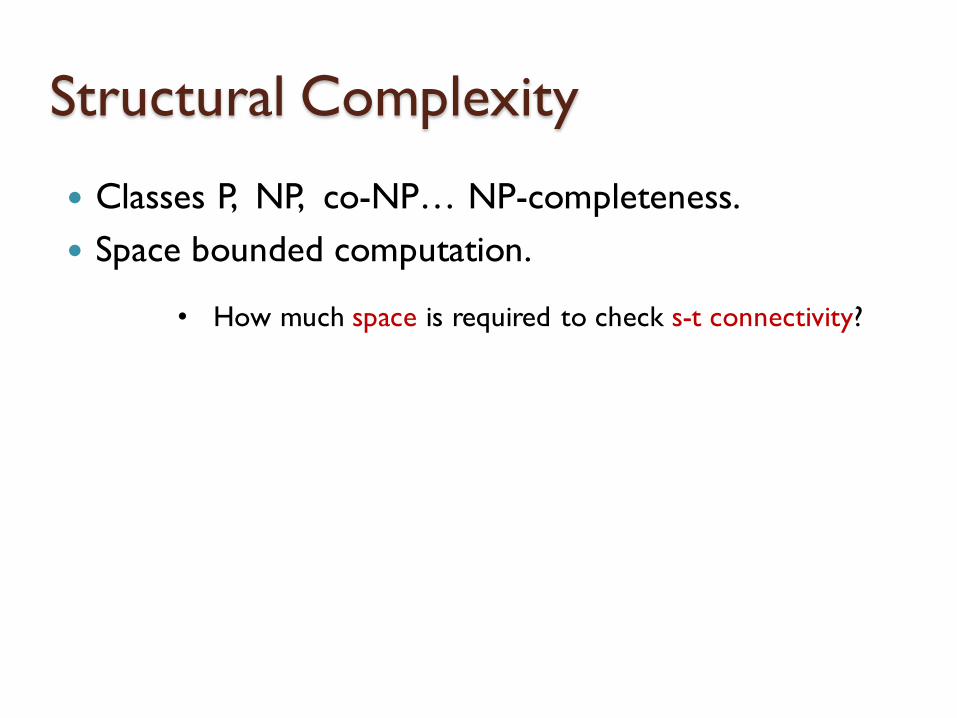
Classes P, NP, co-NP… NP-completeness.
Space bounded computation.
• How much space is required to check s-t connectivity?

Structural Complexity
Classes P, NP, co-NP… NP-completeness.
Space bounded computation.
Polynomial Hierarchy.
co-NP NP
P
.
.
. • How hard is it to check if the largest
independent set in G has size k ?
• How hard is it to check if there is a
circuit of size k that computes the same Boolean function as a given Boolean circuit C ?

Circuit Complexity
The internal workings of an algorithm can be viewed as a Boolean circuit.
The size, depth & width of a circuit correspond to the sequential, parallel & space complexity, respectively, of the algorithm that it represents.

Circuit Complexity
The internal workings of an algorithm can be viewed as a Boolean circuit.
The size, depth & width of a circuit correspond to the sequential, parallel & space complexity, respectively, of the algorithm that it represents.
Proving P≠NP showing circuit lower bounds.
• We will see lower bounds for restricted classes of circuits.

Randomness in Computation
Probabilistic complexity classes.
• Does randomization help in improving efficiency? • Quicksort has O(n log n) expected time but O(n^2) worst
case time. • Can SAT be solved in polynomial time using randomness?
Theorem (Schoening, 1999): 3SAT can be solved in randomized O((4/3)n) time.

Counting Complexity
Counting complexity classes.
• How hard is it to count the number of perfect matchings
in a graph?
• How hard is it to count the number of cycles in a graph? • Is counting much harder than the corresponding decision
problem?

Hardness of Approximation
Probabilistically Checkable Proofs (PCPs).
Hardness of approximation results.
Theorem (Hastad, 1997): If there’s a poly-time algorithm to compute an assignment that satisfies at least 7/8 + e
fraction of the clauses of an input 3SAT, for any constant e > 0, then P = NP.

Basic Course Info
Course title: Computational Complexity Theory
Credits: 3:1 Instructor: Chandan Saha
Lectures: Links to pre-recorded videos will be shared every week.
Weekly interaction: One hour on Google meet. Link will be shared soon.
Primary reference: Computational Complexity – A Modern Approach by Sanjeev Arora and Boaz Barak.

Basic Course Info
Prerequisites: Basic familiarity with algorithms;
Mathematical maturity.
Grading policy: Three Assignments - 45%
One ~45 mins presentation - 25%
One oral exam - 30%
Course homepage: https://www.csa.iisc.ac.in/~chandan/courses/complexity20/home.html

Let’s begin…

Turing Machines
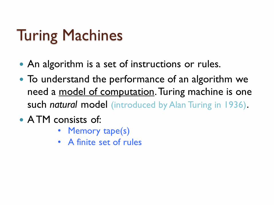
An algorithm is a set of instructions or rules.
To understand the performance of an algorithm we need a model of computation. Turing machine is one such natural model (introduced by Alan Turing in 1936).
Turing Machines
An algorithm is a set of instructions or rules.
To understand the performance of an algorithm we need a model of computation. Turing machine is one such natural model (introduced by Alan Turing in 1936).
A TM consists of:
• Memory tape(s) • A finite set of rules

Turing Machines
An algorithm is a set of instructions or rules.
To understand the performance of an algorithm we need a model of computation. Turing machine is one such natural model (introduced by Alan Turing in 1936).
A TM consists of:
Turing machines A mathematical way to
describe algorithms.
• Memory tape(s) • A finite set of rules

Turing Machines
An algorithm is a set of instructions or rules.
To understand the performance of an algorithm we need a model of computation. Turing machine is one such natural model (introduced by Alan Turing in 1936).
A TM consists of:
(e.g. of a physical realization of a TM is a simple adder)
• Memory tape(s) • A finite set of rules

Turing Machines
Definition. A k-tape Turing Machine M is described by a tuple (Γ, Q, δ) such that

Turing Machines
Definition. A k-tape Turing Machine M is described by a tuple (Γ, Q, δ) such that
M has k memory tapes (input/work/output tapes) with heads;
Γis a finite set of alphabets. (Every memory cell contains an element of Γ)

Turing Machines
Definition. A k-tape Turing Machine M is described by a tuple (Γ, Q, δ) such that
M has k memory tapes (input/work/output tapes) with heads;
Γis a finite set of alphabets. (Every memory cell contains an element of Γ)
has a blank symbol

Turing Machines
Definition. A k-tape Turing Machine M is described by a tuple (Γ, Q, δ) such that
M has k memory tapes (input/work/output tapes) with heads;
Γis a finite set of alphabets. (Every memory cell contains an element of Γ)
Q is a finite set of states. (special states: qstart , qhalt)
δ is a function from Q x Γ to Q x Γ x {L,S,R}
k k k
known as transition function; it captures the dynamics of M

Turing Machines: Computation
Start configuration.
All tapes other than the input tape contain blank symbols.
The input tape contains the input string.
All the head positions are at the start of the tapes.
The machine is in the start state qstart .

Turing Machines: Computation
Start configuration.
All tapes other than the input tape contain blank symbols.
The input tape contains the input string.
All the head positions are at the start of the tapes.
The machine is in the start state qstart .
Computation.
A step of computation is performed by applying δ.
Halting.
Once the machine enters qhalt it stops computation.

Turing Machines: Running time
Let f: {0,1}* {0,1}* and T: and M be a Turing machine.
Definition. We say M computes f if on every x in {0,1}*, M halts with f(x) on its output tape beginning from the start configuration with x on its input tape.

Turing Machines: Running time
Let f: {0,1}* {0,1}* and T: and M be a Turing machine.
Definition. We say M computes f if on every x in {0,1}*, M halts with f(x) on its output tape beginning from the start configuration with x on its input tape.
Definition. M computes f in T(|x|) time, if for every x in {0,1}*, M halts within T(|x|) steps of computation and outputs f(x).

Turing Machines
In this course, we would be dealing with
Turing machines that halt on every input.
Computational problems that can be solved by Turing machines.

Turing Machines
In this course, we would be dealing with
Turing machines that halt on every input.
Computational problems that can be solved by Turing machines.
Can every computational problem be solved using Turing machines?
Turing Machines: Uncomputability
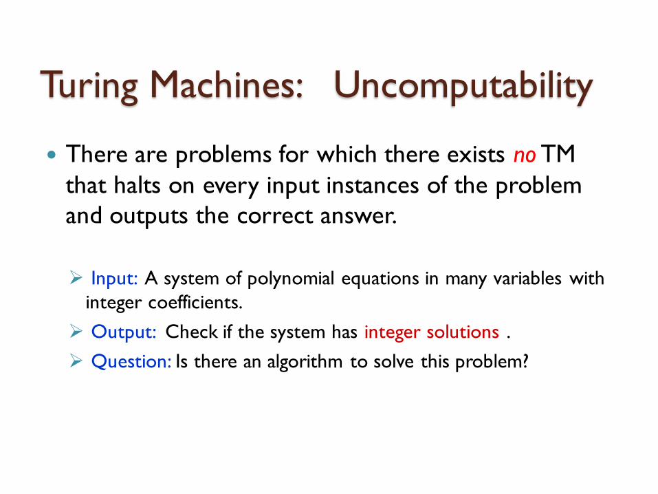
There are problems for which there exists no TM that halts on every input instances of the problem and outputs the correct answer.
Input: A system of polynomial equations in many variables with integer coefficients.
Output: Check if the system has integer solutions .
Question: Is there an algorithm to solve this problem?
Turing Machines: Uncomputability
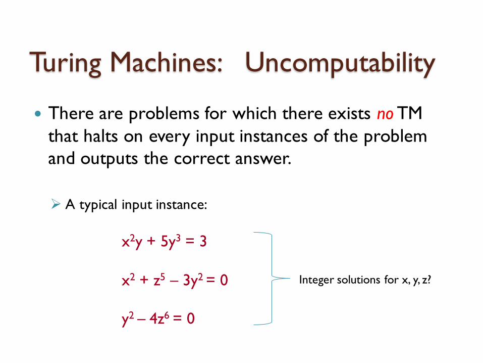
There are problems for which there exists no TM that halts on every input instances of the problem and outputs the correct answer.
A typical input instance:
x2y + 5y3 = 3 x2 + z5 – 3y2 = 0 y2 – 4z6 = 0
Integer solutions for x, y, z?

Turing Machines: Uncomputability
There are problems for which there exists no TM that halts on every input instances of the problem and outputs the correct answer.
Input: A system of polynomial equations in many variables with integer coefficients.
Output: Check if the system has integer solutions .
Question: Is there an algorithm to solve this problem?
(Hilbert’s tenth problem, 1900)

Turing Machines: Uncomputability
There are problems for which there exists no TM that halts on every input instances of the problem and outputs the correct answer.
Input: A system of polynomial equations in many variables with integer coefficients.
Output: Check if the system has integer solutions .
Question: Is there an algorithm to solve this problem?
Theorem. There doesn’t exist any algorithm (realizable by a TM) to solve this problem. (Davis, Putnam, Robinson, Matiyasevich 1970)

Why Turing Machines?
TMs are natural and intuitive.
Church-Turing thesis: “Every physically realizable computation device – whether it’s based on silicon, DNA, neurons or some other alien technology – can be simulated by a Turing machine”.
--- [quoted from Arora-Barak’s book]

Why Turing Machines?
TMs are natural and intuitive.
Church-Turing thesis: “Every physically realizable computation device – whether it’s based on silicon, DNA, neurons or some other alien technology – can be simulated by a Turing machine”.
--- [quoted from Arora-Barak’s book]
Several other computational models can be simulated by TMs.
Possible exception: Quantum machines!

Basic facts about TMs

Turing Machines
Time constructible functions. A function T: is time constructible if T(n) ≥ n and there’s a TM that computes the function that maps x to T(|x|) in O(T(|x|)) time.
Examples: T(n) = n2, or 2n, or n log n
in binary

Turing Machines: Robustness
Let f: {0,1}* {0,1}* and T: be a time constructible function.
Binary alphabets suffice.
If a TM M computes f in T(n) time using Γ as the alphabet set, then there’s another TM M’ that computes f in time 4.log |Γ| . T(n) using {0, 1, blank} as the alphabet set.

Turing Machines: Robustness
Let f: {0,1}* {0,1}* and T: be a time constructible function.
Binary alphabets suffice.
If a TM M computes f in T(n) time using Γ as the alphabet set, then there’s another TM M’ that computes f in time 4.log |Γ| . T(n) using {0, 1, blank} as the alphabet set.
A single tape suffices.
If a TM M computes f in T(n) time using k tapes then there’s another TM M’ that computes f in time 5k . T(n)2 using a single tape that is used for input, work and output.

Turing Machines: As strings
Every TM can be represented by a finite string over {0,1}.
…simply encode the description of the TM.

Turing Machines: As strings
Every TM can be represented by a finite string over {0,1}.
Every string over {0,1} represents some TM.
…invalid strings map to a fixed, trivial TM.

Turing Machines: As strings
Every TM can be represented by a finite string over {0,1}.
Every string over {0,1} represents some TM.
Every TM has infinitely many string representations.
… allow padding with arbitrary number of 0’s

Turing Machines: As strings
Every TM can be represented by a finite string over {0,1}.
Every string over {0,1} represents some TM.
Every TM has infinitely many string representations.
α Mα
{0,1} string TM corresponding to α

Turing Machines: As strings
Every TM can be represented by a finite string over {0,1}.
Every string over {0,1} represents some TM.
Every TM has infinitely many string representations.
A TM (i.e., its string representation) can be given as an input to another TM !!

Universal Turing Machines
Theorem. There exists a TM U that on every input x, α in {0,1}* outputs Mα(x).
Further, if Mα halts within T steps then U halts within C. T. log T steps, where C is a constant that depends only on Mα ’s alphabet size, number of states and number of tapes.

Universal Turing Machines
Theorem. There exists a TM U that on every input x, α in {0,1}* outputs Mα(x).
Further, if Mα halts within T steps then U halts within C. T. log T steps, where C is a constant that depends only on Mα ’s alphabet size, number of states and number of tapes.
Physical realization of UTMs are modern day electronic computers.

Complexity classes P and FP

Decision Problems
In the initial part of this course, we’ll focus primarily on decision problems.

Decision Problems
In the initial part of this course, we’ll focus primarily on decision problems.
Decision problems can be naturally identified with Boolean functions, i.e., functions from {0,1}* to {0,1}.

Decision Problems
In the initial part of this course, we’ll focus primarily on decision problems.
Decision problems can be naturally identified with Boolean functions, i.e., functions from {0,1}* to {0,1}.
Boolean functions can be naturally identified with sets of {0,1} strings, also called languages.

Decision Problems
Decision problems Boolean functions Languages
Definition. We say a TM M decides a language L ⊆ {0,1}* if M computes fL, where fL(x) = 1 if and only if x ∈ L.

Complexity Class P
Let T: be some function.
Definition: A language L is in DTIME(T(n)) if there’s a TM that decides L in time O(T(n)).
Defintion: Class P = ∪ DTIME (nc). c > 0

Complexity Class P
Let T: be some function.
Definition: A language L is in DTIME(T(n)) if there’s a TM that decides L in time O(T(n)).
Defintion: Class P = ∪ DTIME (nc). c > 0
Deterministic polynomial-time

Complexity Class P : Examples
Cycle detection (DFS) Check if a given graph has a cycle.

Complexity Class P : Examples
Cycle detection
Solvabililty of a system of linear equations (Gaussian elimination)
Given a system of linear equations over check if there exists a
common solution to all the linear equations.

Complexity Class P : Examples
Cycle detection
Solvabililty of a system of linear equations
Perfect matching (Edmonds 1965) (birth of class P) Check if a given graph has a perfect matching

Complexity Class P : Examples
Cycle detection
Solvabililty of a system of linear equations
Perfect matching
Planarity testing (Hopcroft & Tarjan 1974) Check if a given graph is planar

Complexity Class P : Examples
Cycle detection
Solvabililty of a system of linear equations
Perfect matching
Planarity testing
Primality testing (Agrawal, Kayal & Saxena 2002)
Check if a number is prime

Polynomial-time Turing Machines
Definition. A TM M is a polynimial-time TM if there’s a polynomial function q: such that for every input x ∈ {0,1}*, M halts within q(|x|) steps.
Polynomial function. q(n) = nc for some constant c
Class (functional) P
What if a problem is not a decision problem? Like the task of adding two integers.

Class (functional) P
What if a problem is not a decision problem? Like the task of adding two integers.
One way is to focus on the i-th bit of the output and make it a decision problem.
(Is the i-th bit, on input x, 1?)

Class (functional) P
What if a problem is not a decision problem? Like the task of adding two integers.
One way is to focus on the i-th bit of the output and make it a decision problem.
Alternatively, we define a class called functional P or FP.

Class (functional) P
What if a problem is not a decision problem? Like the task of adding two integers.
One way is to focus on the i-th bit of the output and make it a decision problem.
We say that a problem or a function f: {0,1}* {0,1}* is in FP (functional P) if there’s a polynomial-time TM that computes f.

Complexity Class FP : Examples
Greatest Common Divisor (Euclid ~300 BC) Given two integers a and b, find their gcd.

Complexity Class FP : Examples
Greatest Common Divisor
Counting paths in a DAG (homework)
Find the number of paths between two vertices in a directed
acyclic graph.

Complexity Class FP : Examples
Greatest Common Divisor
Counting paths in a DAG
Maximum matching (Edmonds 1965) Find a maximum matching in a given graph

Complexity Class FP : Examples
Greatest Common Divisor
Counting paths in a DAG
Maximum matching
Linear Programming (Khachiyan 1979, Karmarkar 1984)
Optimize a linear objective function subject to linear (in)equality constraints

Complexity Class FP : Examples
Greatest Common Divisor
Counting paths in a DAG
Maximum matching
Linear Programming (Khachiyan 1979, Karmarkar 1984)
Optimize a linear objective function subject to linear (in)equality constraints
LP doesn’t have a strongly polynomial-time algorithm. Homework: Read about the differences between strongly poly-time, weakly poly-time and pseudo poly-time algorithms.
Complexity Class FP : Examples
Greatest Common Divisor
Counting paths in a DAG
Maximum matching
Linear Programming
Factoring Polynomials (Lenstra, Lenstra, Lovasz 1982)
Compute the irreducible factors of a univariate polynomial over