Computational Biology, Part 15Biochemical Kinetics I

Computational Biology, Part 15Biochemical Kinetics I

Robert F. MurphyRobert F. Murphy

Copyright Copyright 1996, 1999, 2000, 2001. 1996, 1999, 2000, 2001.

All rights reserved.All rights reserved.

Biochemical KineticsBiochemical Kinetics

The recursion relations we have used before The recursion relations we have used before could be expressed as could be expressed as differendifferencece equations equations..

This is because an equation of the form This is because an equation of the form xxi+1i+1=f(x=f(xii)) can always be rewritten as can always be rewritten as

xxii=f(x=f(xii)-x)-xii

Analysis of the Analysis of the kineticskinetics of biochemical of biochemical reactions requires the use of reactions requires the use of differendifferentialtial equationsequations..

Differential equations vs. difference equationsDifferential equations vs. difference equations A differenA differencece equation expresses the change equation expresses the change

in some variable as a result of a in some variable as a result of a finitefinite change in another variable.change in another variable.

A differenA differentialtial equation expresses the change equation expresses the change in some variable as a result of an in some variable as a result of an infinitesimalinfinitesimal change in another variable. change in another variable.

Difference equationsDifference equations

Difference equations allow direct, Difference equations allow direct, exact exact integrationintegration to calculate the values of to calculate the values of dependent variables at all values of the dependent variables at all values of the independent variable (such as generation independent variable (such as generation number)number)

Difference equations imply a Difference equations imply a “synchronicity” to changes in variables“synchronicity” to changes in variables

Differential equationsDifferential equations

Differential equations can sometimes be Differential equations can sometimes be solved solved analyticallyanalytically to yield an equation for to yield an equation for the dependent variable as a function of the the dependent variable as a function of the independent variable(s) that does not independent variable(s) that does not involve derivativesinvolve derivatives

An alternative is to An alternative is to approximateapproximate the the solution by solution by numerical integrationnumerical integration

Numerical integrationNumerical integration

Numerical integration of differential Numerical integration of differential equations only yields an approximation equations only yields an approximation because we cannot calculate infinitesimal because we cannot calculate infinitesimal changeschanges

We must use a finite We must use a finite integration interval integration interval or or step sizestep size and thereby convert a and thereby convert a differential equation into a difference differential equation into a difference equationequation

Numerical integrationNumerical integration

The simplest numerical integration method The simplest numerical integration method is is Euler’s methodEuler’s method. It simply converts each . It simply converts each differential to a difference and calculates differential to a difference and calculates the value of the dependent variables by the value of the dependent variables by multiplying the right hand side of each multiplying the right hand side of each differential equation by the step size.differential equation by the step size.

Numerical integrationNumerical integration

The smaller the step size is, the greater the The smaller the step size is, the greater the accuracy obtained but the greater the number of accuracy obtained but the greater the number of calculations that must be done to get to a calculations that must be done to get to a specific value of the independent variablespecific value of the independent variable

To increase efficiency, the step size can be To increase efficiency, the step size can be changed from one step to anotherchanged from one step to another If the change in the dependent variable from the If the change in the dependent variable from the

previous step to the current one is “small,” the step previous step to the current one is “small,” the step size can be increased (and vice versa)size can be increased (and vice versa)

GoalGoal

As with the example from population As with the example from population dynamics, our goal is to describe how the dynamics, our goal is to describe how the behavior of a system depends on behavior of a system depends on parameters parameters (e.g., rate constants) and (e.g., rate constants) and boundary conditions boundary conditions (e.g., initial (e.g., initial concentrations)concentrations)

Boundary conditionsBoundary conditions

Boundary conditions can be divided into two Boundary conditions can be divided into two categoriescategories Initial value problems Initial value problems occur when all dependent occur when all dependent

variables are known at some starting value of the variables are known at some starting value of the independent variableindependent variable

Two-point boundary problems Two-point boundary problems occur when some occur when some dependent variables are known only at one value of dependent variables are known only at one value of the independent variable and the rest are known only the independent variable and the rest are known only at some other value of the independent variableat some other value of the independent variable

Initial value problemsInitial value problems

We will consider only initial value We will consider only initial value problems, where we wish to calculate the problems, where we wish to calculate the values of the dependent variables at some values of the dependent variables at some point or set of points different from the point or set of points different from the initial pointinitial point

Example biochemical systemExample biochemical system

For illustration, we will consider a simple, For illustration, we will consider a simple, well-studied biochemical reaction, the well-studied biochemical reaction, the enzyme-catalyzed conversion of a substrate enzyme-catalyzed conversion of a substrate into a productinto a product

E + Sk1→

k−1← C

k2→ E + P

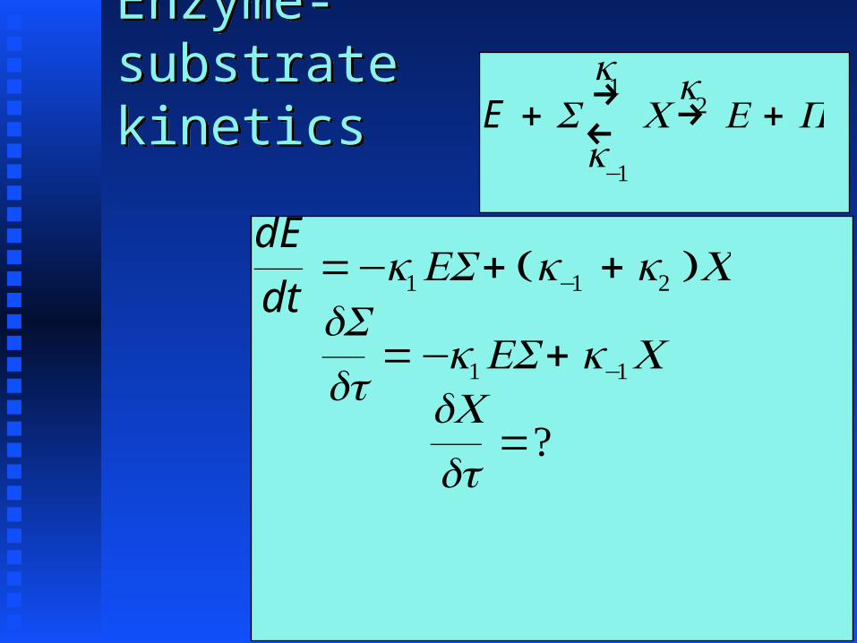
Enzyme-substrate kineticsEnzyme-substrate kinetics

We can write four differential equations We can write four differential equations describing this system. We will use describing this system. We will use EE as as shorthand for shorthand for EE((tt), ), SS for for SS((tt), ), CC for for C C((tt), and ), and PP for for PP((tt).).

What is an expression for What is an expression for dE/dtdE/dt??

E + Sk1→

k−1← C

k2→ E + P

Enzyme-substrate kineticsEnzyme-substrate kinetics E + S

k1→

k−1← C

k2→ E + P

dE

dt=−k1ES+ k−1 + k2( )C

dSdt

=?

dE

dt=−k1ES+ k−1 + k2( )CdSdt

=−k1ES+ k−1CdCdt

=?

Enzyme-substrate kineticsEnzyme-substrate kinetics E + S

k1→

k−1← C

k2→ E + P

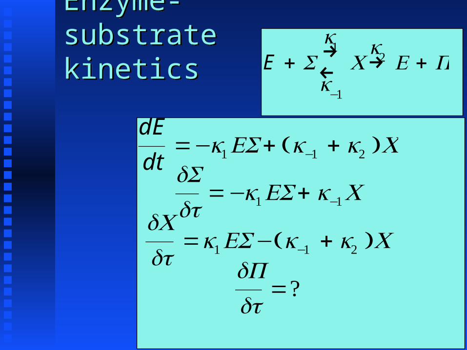
dE

dt=−k1ES+ k−1 + k2( )CdSdt

=−k1ES+ k−1CdCdt

=k1ES− k−1 + k2( )CdPdt

=?

Enzyme-substrate kineticsEnzyme-substrate kinetics E + S

k1→

k−1← C

k2→ E + P

dE

dt=−k1ES+ k−1 + k2( )CdSdt

=−k1ES+ k−1CdCdt

=k1ES− k−1 + k2( )CdPdt

=k2C

Enzyme-substrate kineticsEnzyme-substrate kinetics E + S

k1→

k−1← C

k2→ E + P

Enzyme-substrate kineticsEnzyme-substrate kinetics

Boundary conditionsBoundary conditions

Normally, enzyme and substrate are mixed at time 0, Normally, enzyme and substrate are mixed at time 0, so product and complex concentrations are initially 0: so product and complex concentrations are initially 0: CC00==PP00=0.=0.

E (0 ) = E0

S(0 ) = S0C(0 ) = C0

P(0 ) = P0

What now?What now?

We have a set of four coupled differential We have a set of four coupled differential equations that cannot be solved analytically.equations that cannot be solved analytically.

We canWe can Try to simplify them using various assumptions Try to simplify them using various assumptions

so that they can be solved analytically, orso that they can be solved analytically, or Integrate them numericallyIntegrate them numerically

First simplification: Assumption of substrate excessFirst simplification: Assumption of substrate excess To simplify system, we first assume that the To simplify system, we first assume that the

substrate is present in such a high substrate is present in such a high concentration that it is always in vast excess concentration that it is always in vast excess over the enzyme concentration. In this case, over the enzyme concentration. In this case, the substrate concentration may be viewed the substrate concentration may be viewed as remaining constant:as remaining constant:

S( t ) ≡ S0

Assumption of substrate excessAssumption of substrate excess

Enzyme is either free or in complex. Mass Enzyme is either free or in complex. Mass balance gives an expression for balance gives an expression for EE

Substituting this for Substituting this for EE and and SS00 for for SS in the in the

original differential equation for original differential equation for CC gives gives

E + C = E0 + C0

E = E0 + C0 −C

Assumption of substrate excessAssumption of substrate excess

This can be integrated directly to giveThis can be integrated directly to giveC ( t ) = C0 −C( )e− k1S0 +k−1 +k2( ) t + C

where

C =E0 + C0( )S0Km + S0

and

Km =k−1 + k2

k1

Assumption of substrate excessAssumption of substrate excess

Conclusion: Complex concentration Conclusion: Complex concentration asymptotically approaches the steady-state asymptotically approaches the steady-state concentration, concentration, C

TimescaleTimescale

How long does it take to reach the steady How long does it take to reach the steady state? It must depend on the state? It must depend on the kk’s since they ’s since they are in the term in front of are in the term in front of tt in the exponential. in the exponential.

One characterization of the One characterization of the timescaletimescale of a of a process: How long does it take the function process: How long does it take the function describing the process to go from its describing the process to go from its minimum value to its maximum value if minimum value to its maximum value if going at its maximum rate.going at its maximum rate.

TimescaleTimescale

DefinitionDefinition

timescale ( f ) =fmax − fmin

df

dt max

TimescaleTimescale

In our case, In our case, CC((tt) follows an exponential so ) follows an exponential so we consider we consider ff((tt)=)=ee--ktkt with with kk==kk11SS00++kk-1-1++kk22..

for 0 ≤ t < ∞

fmax = e−k0 =1 andfmin = e−k∞ = 0

dfdt max

= −ke−ktmax

= k

∴ timescale(e−kt ) =1 −0

k= k−1

Timescale and step sizeTimescale and step size

The timescale of a process is a useful guide The timescale of a process is a useful guide to determining the step size for numerical to determining the step size for numerical integration.integration.

A rule of thumb if using a fixed step size is A rule of thumb if using a fixed step size is to set it to no more than one-tenth of the to set it to no more than one-tenth of the timescale.timescale.