arX

iv:1

703.

0605

8v2

[cs

.GT

] 2

5 M

ay 2

018

1

Computation Peer Offloading for

Energy-Constrained Mobile Edge Computing

in Small-Cell Networks

Lixing Chen, Student Member, IEEE,

Sheng Zhou, Member, IEEE, Jie Xu, Member, IEEE

Abstract

The (ultra-)dense deployment of small-cell base stations (SBSs) endowed with cloud-like computing

functionalities paves the way for pervasive mobile edge computing (MEC), enabling ultra-low latency

and location-awareness for a variety of emerging mobile applications and the Internet of Things. To

handle spatially uneven computation workloads in the network, cooperation among SBSs via workload

peer offloading is essential to avoid large computation latency at overloaded SBSs and provide high

quality of service to end users. However, performing effective peer offloading faces many unique

challenges due to limited energy resources committed by self-interested SBS owners, uncertainties in

the system dynamics and co-provisioning of radio access and computing services. This paper develops

a novel online SBS peer offloading framework, called OPEN, by leveraging the Lyapunov technique, in

order to maximize the long-term system performance while keeping the energy consumption of SBSs

below individual long-term constraints. OPEN works online without requiring information about future

system dynamics, yet provides provably near-optimal performance compared to the oracle solution

that has the complete future information. In addition, this paper formulates a peer offloading game

among SBSs, analyzes its equilibrium and efficiency loss in terms of the price of anarchy to thoroughly

understand SBSs’ strategic behaviors, thereby enabling decentralized and autonomous peer offloading

decision making. Extensive simulations are carried out and show that peer offloading among SBSs

dramatically improves the edge computing performance.

L. Chen and J. Xu are with the Department of Electrical and Computer Engineering, University of Miami, USA. Email:

lx.chen@miami.edu, jiexu@miami.edu. S. Zhou is with the Department of Electronic Engineering, Tsinghua University, China.

Email: sheng.zhou@tsinghua.edu.cn.

2

I. INTRODUCTION

Pervasive mobile devices and the Internet of Things are driving the development of many new

applications, turning data and information into actions that create new capabilities, richer experi-

ences and unprecedented economic opportunities. Although cloud computing enables convenient

access to a centralized pool of configurable and powerful computing resources, it often cannot

meet the stringent requirements of latency-sensitive applications due to the often unpredictable

network latency and expensive bandwidth [1]–[3]. The growing amount of distributed data

further makes it impractical or resource-prohibitive to transport all the data over today’s already-

congested backbone networks to the remote cloud [4]. As a remedy to these limitations, mobile

edge computing (MEC) [1]–[3] has recently emerged as a new computing paradigm to enable

in-situ data processing at the network edge, in close proximity to mobile devices and connected

things. Located often just one wireless hop away from the data source, edge computing provides a

low-latency offloading infrastructure, and an optimal site for aggregating, analyzing and distilling

bandwidth-hungry data from end devices.

!"#$!"#$!"#$%&$'(&)*

+,-

./.

0##$1&22(&)*345

6)7$&1/.

%3$#(#""1(34'

%3$#*1080

+,-

Fig. 1. Illustration of SBS peer offloading.

Considered as a key enabler of MEC, small-cell base stations (SBSs), such as femtocells

and picocells, endowed with cloud-like computing and storage capabilities can serve end users’

computation requests as a substitute of the cloud [3]. Nonetheless, compared to mega-scale

data centers, SBSs are limited in their computing resources. Since the computation workload

arrivals in small cell networks can be highly dynamic and heterogeneous, it is very difficult

for an individual SBS to provide satisfactory computation service at all times. To overcome

3

these difficulties, cooperation among SBSs can be exploited to enhance MEC performance

and improve the efficiency of system resource utilization via computation peer offloading. For

instance, a cluster of SBSs can coordinate among themselves to serve mobile users by offloading

computation workload from SBSs located in hot spot areas to nearby peer SBSs with light

computation workload, thereby balancing workload among the geographically distributed SBSs

(see Figure 1 for an illustration). Similar ideas have been investigated for data-center networks

to deal with spatial diversities of workload patterns, temperatures, and electricity prices. In

fact, SBS networks are more vulnerable to heterogeneous workload patterns than data center

networks which serve an aggregation of computation requests across large physical regions. Since

the serving area of each SBS is small, the workload pattern can be affected by many factors

such as location, time, and user mobility, therefore becoming very violate and easily leading to

uneven workload distribution among the SBSs. Although there have been quite a few works on

geographical load balancing in data centers, performing peer offloading in MEC-enabled small

cell networks faces unique challenges.

First, small cells are often owned and deployed by individual users. Although incentive

mechanism design, which has been widely studied in the literature for systems not limited to

small cell networks, plays an important role in incentivizing self-interested users to participate

in the collaboration of workload peer offloading, an equally, if not more, important problem

is how to maximize the value of the limited resources committed by individual SBS owners.

Second, small cells operate in a highly stochastic environment with random workload arrivals

in both temporal and spatial domains. As a result, the long-term system performance is more

relevant than the immediate performance. However, the limited energy resources committed by

the SBS owners make the peer offloading decisions across time intricately intertwined, yet the

decisions have to be made without foreseeing the far future. Third, whereas data centers manage

only the computing resources, moving the computing resources to the network edge leads to

the co-provisioning of radio access and computing services by the SBSs, thus mandating a new

model for understanding the interplay and interdependency between the management of the two

resources under energy constraints.

In this paper, we study computation peer offloading in MEC-enabled small cell networks.

Our goal is to maximize the long-term system-wide performance (i.e. minimizing latency) while

taking into account the limited energy resources committed by individual SBS owners. The main

contributions of this paper are summarized as follows:

4

1) We develop a novel framework called OPEN (which stands for Online PEer OffloadiNg) for

performing stochastic computation peer offloading among a network of MEC-enabled SBSs in an

online fashion by leveraging the Lyapunov optimization [5]. We prove that OPEN achieves within

a bounded deviation from the optimal system performance that can be achieved by an oracle

algorithm that knows the complete future information, while bounding the potential violation of

the energy constraints imposed by individual SBS owners.

2) We theoretically characterize the optimal peer offloading strategy. We show that the peer

offloading decisions are determined by the marginal computation cost (MaCC) – a critical

quantity that captures both computation delay cost and energy cost at SBSs. The peer offloading

essentially is to evenly distribute MaCCs among SBSs. The SBSs decide their roles (to send

or receive workload) based on the pre-offloading MaCCs (i.e., MaCCs before peer offloading).

The amount of workload to be offloaded is determined based on optimal post-offloading MaCCs

(i.e., MaCCs to achieve after peer offloading) designed by OPEN.

3) We consider both the scenario in which a central entity (e.g. the network operator) collects

all current time information and coordinates the peer offloading and the scenario in which SBSs

coordinate their peer offloading strategies in a decentralized and autonomous way. For the latter

case, we formulate a novel peer offloading game, prove the existence of a Nash equilibrium

using the variational inequality technique, and characterize the efficiency loss due to the strategic

behaviors of SBSs in terms of the price of anarchy (PoA).

4) We run extensive simulations to evaluate the performance of OPEN and verify our analytical

results for various system configurations and traffic arrival patterns. The results confirm that our

method significantly improves the system performance in terms of latency reduction and energy

efficiency.

The rest of this paper is organized as follows. Section II reviews related works. Section III

presents the system model and formulates the problem. Section IV develops the OPEN framework

and presents the centralized solution for computation peer offloading. Section V formulates and

analyzes the peer offloading game. Simulations are carried out in Section VI, followed by the

conclusion in Section VII.

II. RELATED WORK

The concept of offloading data and computation in cloud computing is used to address the

inherent problems in mobile computing by using resource providers other than the mobile device

5

TABLE I

COMPARISON WITH EXISTING WORKS

Feature

Approach[6], [7] [8]–[10] [11] [12] [13] [14], [15] OPEN (This paper)

Applied stage UE-to-ES UE-to-ES DC-to-DC DC-to-DC UE-to-DC UE-to-ES ES-to-ES

Radio access aware Yes Yes No No No Yes Yes

Computation aware No Yes Yes Yes Yes Yes Yes

System objective Myopic Myopic Long-term Myopic Long-term Myopic Long-term

Long-term constraints No No Yes (Overall) No No No Yes (Individual)

Temporal correlation No No Yes No Yes No Yes

Strategic behavior No No No No Yes Yes Yes

UE: User equipment; DC: Data Center; ES: Edge Server

itself to host the execution of mobile applications [16]. In the most common case, mobile

cloud computing means to run an application on a resource rich cloud server located in remote

mega-scale data centers, while the mobile device acts like a thin client connecting over to the

remote server through 4G/Internet [17]. Recently, the edge computing paradigm [2] (a.k.a. fog

computing [18], cloudlet [19], micro datacenter [20]) brings computing resources closer to the

end users to enable ultra-low latency and precise location-awareness, thereby supporting a variety

of emerging mobile applications such as mobile gaming, augmented reality and autonomous

vehicles. Nevertheless, edge servers, such as MEC-enabled SBSs [21], cannot offer the same

computation and storage capacities as traditional computing servers.

Many recent works investigate SBS cooperation for improving the system performance, subject

to various constraints including local resource availability (e.g. radio resources [6], [7], com-

putational capacities [10], energy consumption budgets [22] and backhaul bandwidth capacity

[23]). However, most of these works focus on optimizing the radio access performance only

without considering the computing capability of SBSs. In [9], [10], computation load distribu-

tion among the network of SBSs is investigated by considering both radio and computational

resource constraints. Clustering algorithms are proposed to maximize users’ satisfaction ratio

while keeping the communication power consumption low. However, these works focus more

on the user-to-SBS offloading side whereas our paper studies the offloading among peer SBSs.

More importantly, these works perform myopic optimization without considering the stochastic

nature of the system whereas our paper studies a problem that is highly coupled across time due

to the long-term energy constraints.

6

Computation workload peer offloading among SBSs is closely related to geographical load

balancing techniques originally proposed for data centers to deal with spatial diversities of

workload patterns [24], temperatures [25], and electricity prices [26]. Most of these works

study load balancing problems that are independent across time [27]. Very few works consider

temporally coupled problems. In [24], the temporal dependency is due to the switching costs

(turning on/off) of data center servers, which significantly differs from our considered problem.

The closest work to our paper is [11], which aims to minimize the long-term operational cost

of data centers subject to a long-term water consumption constraint. However, the long-term

constraint is imposed on the entire system whereas in our paper each SBS has an individual

energy budget constraint. Moreover, we not only provide centralized solutions for peer-offloading

but also develop schemes that enable autonomous coordination among SBSs by formulating and

studying a peer-offloading game. Several works use reinforcement learning to efficiently manage

the resource of geo-distributed data centers [28], [29]. Although the reinforcement learning can

also be a potential solution to our peer-offloading problem, there are several challenges for using

such a formulation. First, the system states are usually assumed to be Markovian, which may

not be true in real systems. Second, large state and action spaces may be needed to capture

the various system and decision variables and hence complexity and convergence is a big issue.

Third, reinforcement learning often does not capture the long-term energy constraint and may

easily violate it. By contrast, our solution is based on the Lyapunov drift-plus-penalty framework,

which can be applied to more general stochastic systems, does not need to maintain large state

and action spaces, and can handle long-term energy constraints.

The formulated peer offloading game is similar to the widely studied congestion game [30] at

the first sight. However, there is a crucial difference between these two games: a main assumption

in congestion games is that all players have the same cost function for a element; however, in the

peer offloading game, cost function of a SBS to retain workload on itself is different from that of

other SBSs to offload tasks to that SBS due to the energy consumption concern. This difference

demands for new analytical tools for understanding the peer offloading game. For instance, the

potential function technique [30] used to establish the existence of a Nash equilibrium in the

congestion game does not apply and hence, in this paper, we prove the existence of a Nash

equilibrium via the variational inequality technique [31]. Game theoretic modeling was also

applied in the MEC computation offloading context in [14] [15]. This work focuses on the

computation offloading among multiple UEs to a single BS, which is a different scenario than

7

ours. Table 1 summarizes the differences of proposed strategy from existing works.

III. SYSTEM MODEL

A. Network model

We consider N SBSs (e.g. femtocells), indexed by N = 1, . . . , N, deployed in a building

(residential or enterprise) and connected by the same Local Area Network (LAN). These SBSs

are endowed with, albeit limited, edge computing capabilities and hence, User Equipments (UEs)

can offload their computation tasks to corresponding serving SBSs via wireless communications

for processing. The computing capabilities of SBS i is characterized by its computation service

rate fi (CPU frequency), and the computation service rates of all SBSs in the network are

collected by f = fii∈N . Let M = 1, . . . ,M denote the set of all UEs in the building. Each

SBS serves a dedicated set of UEs in its serving area, denoted by Mi ⊆ M. For example,

UEs (e.g. mobile phones, laptops etc.) of employees in a business are authorized to access

the communication/computing service of the SBS deployed by the business. Notice that our

algorithm is also compatible with other network structure and association strategies as long as

the UE-SBS associations stay unchanged in one peer offloading decision cycle.

B. Workload arrival model

The operational timeline is discretized into time slots (e.g. 1 - 5 minutes) for making peer

offloading decisions, which is a much slower time scale than that of task arrivals. In each time

slot t, computation tasks originating from UE m is generated according to a Poisson process

which is a common assumption on the computation task arrival in edge systems [1]. Let πtm

denote the rate of the Poisson process for task generation at UE m in time slot t. In each time

slot, πtm is randomly drawn from πt

m ∈ [0, πmax] to capture the temporal variation in task arrival

pattern. Let πt = πtmm∈M denote the task arrival pattern of all UEs in time slot t. The UEs

may request for different types of tasks which vary in input date size and required CPU cycles.

To simply the system model, we assume that the expected input data size for one task is s (in

bits) and the expected number of CPU cycles required by one task is h. The total task arrival

rate to SBS i, denoted by φti, is φt

i =∑

m∈Miπtm. The task arrival rates to all SBSs are collected

in φt = φtii∈N .

8

C. Transmission model

1) Transmission energy consumption: Transmissions occur on both the wireless link between

UEs and SBSs, and the wired link among SBSs. Usually the energy consumption of wireless

transmission dominates and hence we consider only the wireless part. In each time slot t, SBSs

have to serve both uplink and downlink traffic data. We assume that the uplink and downlink

transmission operate on orthogonal channels and focus on the downlink traffic since energy

consumption of SBSs is mainly due to downlink transmission. Suppose each SBS i ∈ N operates

at a fixed transmission power P di , then the achievable downlink transmission rate rd,tim between

UE m and SBS i is given by the Shannon capacity,

rd,tim = W log2

(

1 +P di H

tim

σ2

)

, (1)

where W is the channel bandwidth, H tim is the channel gain between SBS i and UE m,

and σ2 is the noise power. The downlink traffic consists of the computation result and other

communication traffic. Since the size of computation result is usually very small, we only

consider the communication traffic. Let the downlink traffic size in time slot t be wtm ∈ [0, wmax],

then the energy consumption of SBS i for wireless transmission is

E tx,ti =

∑

m∈Mi

P di w

tm

rd,tim

. (2)

2) UE-to-SBS transmission delay: The transmission delay is incurred during UE-to-SBS

offloading where UEs send computation tasks to the SBSs through the uplink channel. Let

P um be the transmission power of UE m, then the uplink transmission rate between UE m and

SBS i, denoted by ru,tim, can be obtained similarly as in (1). Therefore, the total transmission

delay cost for UEs covered by SBS i can be calculated as

Du,ti =

∑

m∈Mi

sπtm

ru,tim

. (3)

D. SBS Peer Offloading

Since workload arrivals are often uneven among the SBSs, computation offloading between

peer SBSs can be enabled to exploit underused, otherwise wasted, computational resource to

improve the overall system efficiency. We assume that tasks can be offloaded only once: if a

task is offloaded from SBS i to SBS j, then it will be processed at SBS j and will not be offloaded

further or back to SBS i to avoid offloading loops. Let βti· = β

tijj∈N denote the offloading

9

decision of SBS i in time slot t, where βtij denotes the fraction of received tasks offloaded from

SBS i to SBS j (notice that βtii is the fraction that SBS i retains). A peer offloading profile of

the whole system is therefore βt = βti·i∈N . We further define βt

·i = βtjij∈N as the inbound

tasks of SBS i, namely the tasks offloaded to SBS i from other SBSs. Clearly, the total workload

that will be processed by SBS i is ωti(β

t) ,∑

j∈N βtji. To better differentiate the two types of

workload φti and ωt

i(βt), we call φt

i the pre-offloading workload and ωti(β

t) the post-offloading

workload. A profile βt is feasible if it satisfies:

1) Positivity: βtij ≥ 0, ∀i, j ∈ N . The offloaded workload must be non-negative.

2) Conservation:∑N

j=1 βtij = φt

i, ∀i ∈ N . The total offloaded workload (including the retained

workload) by each SBS must equal its pre-offloading workload.

3) Stability: ωti(β

t) ≤ fi/h, ∀i ∈ N . The post-offloading workload of each SBS must not

exceed its service rate.

Let Bt denote the set of all feasible peer offloading profile.

Since the bandwidth of the LAN is limited, peer offloading also causes additional delay due to

network congestion. We assume that the expected congestion delay depends on the total traffic

through the LAN, denoted by λt(βt) =∑

i∈N λti(βt), where λti(β

t) =∑

j∈N\i βij = φti−β

tii is

the number of tasks offloaded to other SBSs from SBS i. We assume the data size of computation

tasks has a exponential distribution, then the congestion delay Dg,t is modeled as a M/M/1

queuing system [32]:

Dg,t(βt) =τ

1− τλt(βt), λt <

1

τ, (4)

where τ is the expected delay for sending and receiving s bits (i.e., expected input data size of

a computation task) over the LAN without congestion.

E. Computation model

1) Computation delay: The computation delay is due to the limited computing capability of

SBSs. UEs in the network may request different types of services, therefore the required number

of CPU cycles to process a computation task may vary across tasks. We model the distribution of

the required number of CPU cycles of individual tasks as an exponential distribution. Given the

constant processing rate, the service time of a task therefore follows an exponential distribution.

Further considering the Poisson arrival of the computation tasks, the computation delay at each

10

SBS can be modeled as an M/M/1 queuing system [32] and the expected computation delay

Df,ti for one task at SBS i is:

Df,ti (βt) =

1

µi − ωti(β

t), (5)

where µi = fi/h is the expected service rate with regard to the number of tasks (i.e. tasks per

second) and ωti(β

t) is the workload processed at SBS i given the peer offloading decision βt.

Figure 2 illustrates the relation between the computation delay and the congestion delay.

SBS i SBS j SBS k

kj

i

i

ii

ij

edge server i

LAN

ij

kj

traffic congestion

ij

kj

j j

edge server j

ij

i j k

Computation delay (SBS i) Network congestion delay Computation delay (SBS j)

f

iDgD

f

jD1/

Fig. 2. Illustration of system delay with queuing models. The figure gives a example of network with three SBSs, where SBS

i and SBS k offload workload βij and βkj to SBS j, respectively. The computation delay model for SBS k is omitted since it

is the same as that for SBS i.

2) Computation energy consumption: The computation energy consumption at SBS i is load-

dependent, denoted as Ec,ti . In this paper, we consider a linear computation energy consumption

function Ec,ti (βt) = κ · ωt

i(βt), where κ > 0 is the energy consumption for executing h (i.e.,

expected number of CPU cycles required by a computation task) CPU cycles.

F. Problem Formulation

Peer offloading relies on SBSs’ cooperative behavior in sharing their computing resources

as well as their energy costs. A large body of literature was dedicated to design incentive

mechanisms [33], [34] to encourage cooperation among self-interested SBSs (e.g. computing

capability, energy budget) to improve the social welfare. The focus of our paper is not to design

yet another incentive mechanism. Instead, we design SBS peer offloading strategies taking the

SBS committed resources as the input and hence our method can work in conjunction with any

existing incentive/cooperation mechanisms. Usually, the decision cycle of the resource scheduling

11

is much longer than that of peer offloading, therefore in this paper we consider each SBS has a

predetermined long-term energy consumption constraint as a result of some incentive mechanism.

Given the system model, the total delay cost of SBS i, defined as a sum of the delays expe-

rienced by the tasks arrived at SBSs i, consists of computation delay cost, network congestion

delay cost, and UE-to-SBS transmission delay cost:

Dti(β

t) =∑

j∈N

βtijD

f,tj (βt) + λtiD

g,t(βt) +Du,ti

=∑

j∈N

βtij

µj −∑

k∈N βtkj

+τλti(β

t)

1− τ∑

k∈N λtk(βt)

+Du,ti ,

(6)

and the energy consumption of SBS i in time slot t consists of transmission energy consumption

and computation energy consumption:

Eti(β

t) = E tx,ti + Ec,t

i (βt) = E tx,ti + κ

∑

k∈N

βtki. (7)

The objective of network operator is to minimize the long-term system delay cost given the

energy budgets committed by individual SBSs (which are outcomes of the adopted incentive

mechanisms). Formally, the problem is

P1 minβ1,...,βT−1

1

T

T−1∑

t=0

N∑

i=1

EDt

i(βt)

(8a)

s.t.1

T

T−1∑

t=0

EEt

i (βt)≤ Ei, ∀i ∈ N (8b)

Eti (β

t) ≤ Emax, ∀i ∈ N , ∀t (8c)

Dti(β

t) ≤ Dmax, ∀i ∈ N , ∀t (8d)

βt ∈ Bt, ∀t (8e)

Constraint (8b) is the long-term energy budget constraint for each SBS. Constraint (8c) requires

that the energy consumption of a SBS does not exceed an upper limit Emax in each time slot.

Constraint (8d) indicates that the per-slot delay of each SBS is capped by an upper limit Dmax

so that the real-time performance is guaranteed in the worst case.

The major challenge that impedes the derivation of optimal solution to P1 is the lack of future

information. Optimally solving P1 requires complete offline information (task arrivals across all

time slots) which is difficult to predict in advance, if not impossible. Moreover, the long-term

energy constraints couple the peer offloading decision across different slots: consuming more

12

energy in the current slot will reduce the available energy for future use. These challenges call for

an online optimization approach that can efficiently perform peer offloading without foreseeing

the future.

IV. ONLINE SBS PEER OFFLOADING

In this section, we develop a novel framework for making online SBS peer offloading de-

cisions, called OPEN (Online SBS PEer offloadiNg) by leveraging the Lyapunov technique.

OPEN converts P1 to per-slot optimization problems solvable with only current information.

We consider both the case in which the network operator coordinates the SBS peer offloading

in a centralized way (this section) and the case in which SBSs make peer offloading decisions

among themselves in an autonomous manner (next section).

A. Lyapunov optimization based online algorithm

In the optimization problem P1, the long-term energy constraints of SBSs couple the peer

offloading decisions across times slots. To address this challenge, we leverage the Lyapunov

drift-plus-penalty technique [5] and construct a (virtual) energy deficit queue for each SBS to

guide the peer offloading decisions to follow the long-term energy constraints. We define a set

of energy deficit queues q(t) = qi(t)i∈N , one for each SBS, and let qi(0) = 0, ∀i ∈ N . For

each SBS i ∈ N , its energy deficit queue evolves as follows:

qi(t+ 1) = maxqi(t) + Eti (β

t)− Ei, 0, (9)

where qi(t) is the queue length in time slot t, indicating the deviation of current energy con-

sumption from the long-term energy constraint of SBS i.

Next, we present the online algorithm OPEN (Algorithm 1) for solving P1. In OPEN, the

network operator determines the peer offloading strategy in each time slot t by solving the

optimization problem P2, as presented below:

P2 minβt∈Bt

N∑

i=1

(V ·Dt

i(βt) + qi(t) ·E

ti (β

t))

s.t. (8c), (8d) and (8e)

The objective in P2 is designed based on Lyapunov drift-plus-penalty framework. The rationale

behind this design will be explained later in Section IV-C. The first term in P2 is to minimize the

13

Algorithm 1: OPEN

Input: control parameter V , energy deficit queues q(0) = 0;

Output: offloading decisions β0, . . . ,βT−1;

1 for t = 0 to T − 1 do

2 Observe workload arrival φt and feasible peer offloading strategy set Bt ;

3 Solving P2 to get optimal βt in time slot t:

minβt∈Bt

∑

i∈N

(V ·Dti(β

t) + qi(t) · Eti (β

t)) ;

4 Update the deficit for all SBS i:

5 qi(t+ 1) = [qi(t) + Eti (β

t)− Ei]+

6 end

7 return β1, . . . ,βT−1;

system delay and the second term is added aiming to satisfy the long-term energy constraint (8b)

in an online manner; the positive control parameter V is used to adjust the trade-off between these

two purposes. To give a brief explanation, by considering the additional term∑N

i=1 qi(t)Eti(β

t),

the network operator takes into account the energy deficits of SBSs in current-slot decision

making: when q(t) is larger, minimizing the energy deficits is more critical for network operator.

Thus, OPEN works following the philosophy of “if violate the energy budget, then use less

energy”, and hence the long-term energy constraint can be satisfied in the long run without

foreseeing the future information. Later in this section, we will rigorously prove the performance

of OPEN in terms of system delay cost and long-term energy consumption. Now, to complete

OPEN, it remains to solve the optimization problem P2. Notice that solving P2 requires only

currently available information as input.

B. Centralized solution to OPEN

In this subsection, we consider the existence of a centralized controller who collects the

complete current-slot information from all SBSs, solves the per-slot problem P2, and coordinates

SBS peer offloading in each time slot t. Before proceeding to the solution, we rewrite the

14

objective function of P2 as below:

∑

i∈N

(V ·Dt

i(βt) + qi(t) · E

ti (β

t))

=∑

i∈N

V · (∑

j∈N

βtijD

f,tj (βt) + λti(β

t)Dg,t(βt) +Du,ti ) +

∑

i∈N

qi(t)(Etx,ti + Ec,t

i (βt))

=∑

j∈N

V∑N

i=1 βtij

µj −∑N

k=1 βtkj

+V τ∑N

i=1 λti(β

t)

1− τ∑N

k=1 λtk(β

t)+∑

i∈N

κqi(t)ωti(β

t) +∑

i∈N

(V Du,t

i + qi(t)Etx,ti

)

=∑

i∈N

V

(V ωt

i(βt)

µi − ωti(β

t)+ κqi(t)ω

ti(β

t)

)

+V τλt(βt)

1− τλt(βt)︸ ︷︷ ︸

decision-dependent

+∑

i∈N

(V Du,t

i + qiEtx,ti

)

︸ ︷︷ ︸

decision-independent

. (10)

The objective function of P2 can be divided into two parts: (i) a decision-dependent part which

is a weighted sum of the computation delay cost, the computation energy consumption, and the

network congestion delay cost; (ii) a decision-independent part which relates to the UE-to-SBS

transmission delay and SBS-to-UE energy consumption. Therefore, we focus on the decision-

dependent part for solving P2. Although the decision-independent part does not affect the solution

of P2 directly, its second term (i.e., E tx,t) will affect the energy deficit queue updating and hence

indirectly affects peer offloading decisions in the long-run.

Notice that P2 is solved in each time slot, for ease of exposition, we drop the time index for

variables. Moreover, instead of optimizing βt directly, we alternatively optimize the amount of

workload ωti(β) each SBS should accommodate, and the corresponding total traffic in the LAN

λt(β). By rewriting ωti(β) as ωi and λt(β) as λ, P2 is therefore equivalent to:

P2-S minωi∈Ωi,λ∈Λ

∑

i∈N

(V ωi

µi − ωi

+ κqiωi

)

+V τλ

1− τλ(11a)

s.t. Ei(ωi, λ) ≤ Emax, ∀i ∈ N (11b)

Di(ωi, λ) ≤ Dmax, ∀i ∈ N (11c)

ωi ∈ Ωi, λ ∈ Λ, ∀i ∈ N (11d)

where Ωi in (11d) is the feasible space for ωi determined by the mapping ωi : B → Ωi,

and similarly Λ is determined by λ : B → Λ. Notice that, although ωis and λ are written as

independent variables, they are deterministic functions of a particular β in each time slot. To

capture the relation between ωis and λ, we introduce and closely follow a workload flow equation

when solving P2-S, which will be shown shortly.

15

Next, we give the optimal solution for the above optimization problem starting with classifying

SBSs into the following three categories:

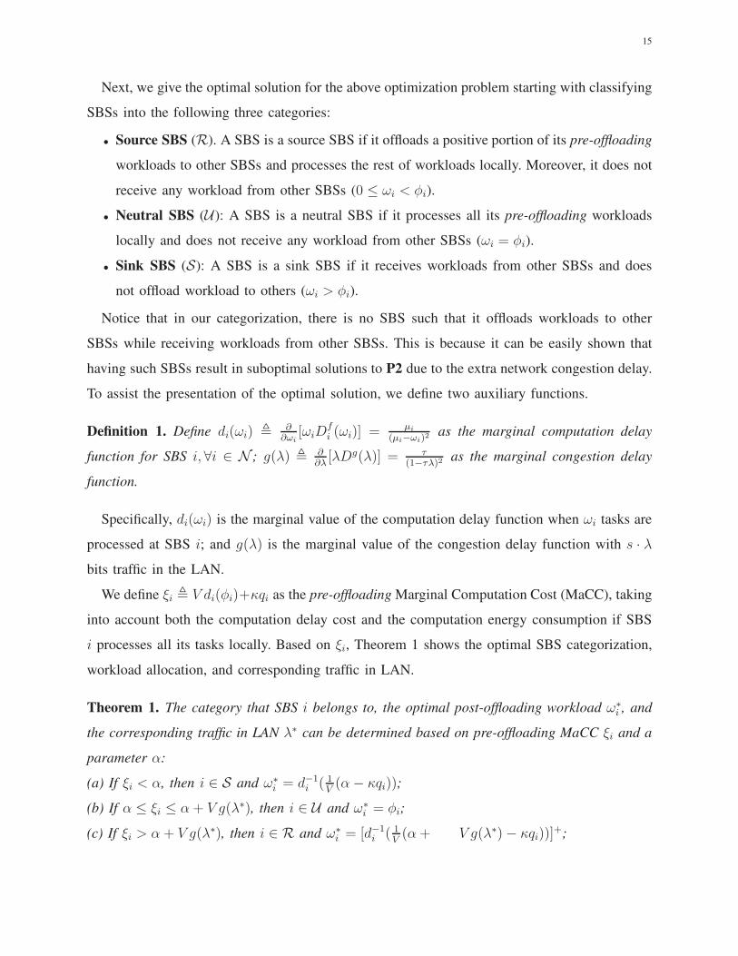
• Source SBS (R). A SBS is a source SBS if it offloads a positive portion of its pre-offloading

workloads to other SBSs and processes the rest of workloads locally. Moreover, it does not

receive any workload from other SBSs (0 ≤ ωi < φi).

• Neutral SBS (U): A SBS is a neutral SBS if it processes all its pre-offloading workloads

locally and does not receive any workload from other SBSs (ωi = φi).

• Sink SBS (S): A SBS is a sink SBS if it receives workloads from other SBSs and does

not offload workload to others (ωi > φi).

Notice that in our categorization, there is no SBS such that it offloads workloads to other

SBSs while receiving workloads from other SBSs. This is because it can be easily shown that

having such SBSs result in suboptimal solutions to P2 due to the extra network congestion delay.

To assist the presentation of the optimal solution, we define two auxiliary functions.

Definition 1. Define di(ωi) , ∂∂ωi

[ωiDfi (ωi)] = µi

(µi−ωi)2as the marginal computation delay

function for SBS i, ∀i ∈ N ; g(λ) , ∂∂λ[λDg(λ)] = τ

(1−τλ)2as the marginal congestion delay

function.

Specifically, di(ωi) is the marginal value of the computation delay function when ωi tasks are

processed at SBS i; and g(λ) is the marginal value of the congestion delay function with s · λ

bits traffic in the LAN.

We define ξi , V di(φi)+κqi as the pre-offloading Marginal Computation Cost (MaCC), taking

into account both the computation delay cost and the computation energy consumption if SBS

i processes all its tasks locally. Based on ξi, Theorem 1 shows the optimal SBS categorization,

workload allocation, and corresponding traffic in LAN.

Theorem 1. The category that SBS i belongs to, the optimal post-offloading workload ω∗i , and

the corresponding traffic in LAN λ∗ can be determined based on pre-offloading MaCC ξi and a

parameter α:

(a) If ξi < α, then i ∈ S and ω∗i = d−1

i ( 1V(α− κqi));

(b) If α ≤ ξi ≤ α + V g(λ∗), then i ∈ U and ω∗i = φi;

(c) If ξi > α + V g(λ∗), then i ∈ R and ω∗i = [d−1

i ( 1V(α+ V g(λ∗)− κqi))]

+;

16

where λ∗, α are the solution to the workload flow equation

∑

i∈S

(

d−1i (

1

V(α− κqi))− φi

)

︸ ︷︷ ︸

λS : inbound workloads to sinks

=∑

i∈R

(

φi − [d−1i (

1

V(α+ V g(λ∗)− κqi))]

+

)

︸ ︷︷ ︸

λR: outbound workloads from sources

. (12)

Proof. See Appendix A in Supplementary File.

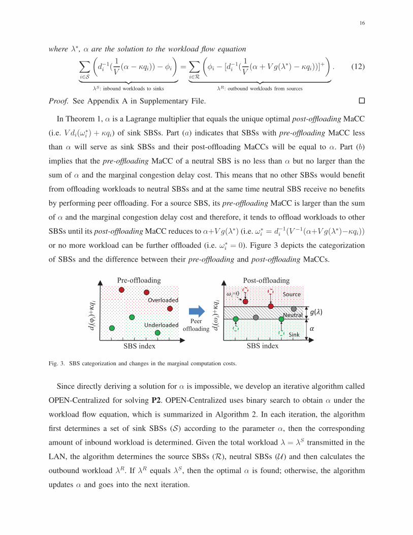
In Theorem 1, α is a Lagrange multiplier that equals the unique optimal post-offloading MaCC

(i.e. V di(ω∗i ) + κqi) of sink SBSs. Part (a) indicates that SBSs with pre-offloading MaCC less

than α will serve as sink SBSs and their post-offloading MaCCs will be equal to α. Part (b)

implies that the pre-offloading MaCC of a neutral SBS is no less than α but no larger than the

sum of α and the marginal congestion delay cost. This means that no other SBSs would benefit

from offloading workloads to neutral SBSs and at the same time neutral SBS receive no benefits

by performing peer offloading. For a source SBS, its pre-offloading MaCC is larger than the sum

of α and the marginal congestion delay cost and therefore, it tends to offload workloads to other

SBSs until its post-offloading MaCC reduces to α+V g(λ∗) (i.e. ω∗i = d−1

i (V −1(α+V g(λ∗)−κqi))

or no more workload can be further offloaded (i.e. ω∗i = 0). Figure 3 depicts the categorization

of SBSs and the difference between their pre-offloading and post-offloading MaCCs.

di(φi)

+qi

SBS index

Pre-offloading

di(ωi)

+qi

SBS index

!"

#$

Post-offloading

%#&

i=0

Peer

offloading

Fig. 3. SBS categorization and changes in the marginal computation costs.

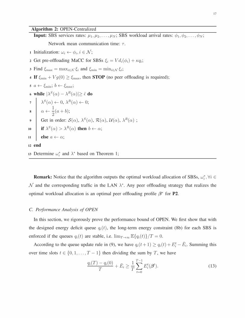
Since directly deriving a solution for α is impossible, we develop an iterative algorithm called

OPEN-Centralized for solving P2. OPEN-Centralized uses binary search to obtain α under the

workload flow equation, which is summarized in Algorithm 2. In each iteration, the algorithm

first determines a set of sink SBSs (S) according to the parameter α, then the corresponding

amount of inbound workload is determined. Given the total workload λ = λS transmitted in the

LAN, the algorithm determines the source SBSs (R), neutral SBSs (U) and then calculates the

outbound workload λR. If λR equals λS, then the optimal α is found; otherwise, the algorithm

updates α and goes into the next iteration.

17

Algorithm 2: OPEN-Centralized

Input: SBS services rates: µ1, µ2, . . . , µN ; SBS workload arrival rates: φ1, φ2, . . . , φN ;

Network mean communication time: τ .

1 Initialization: ωi ← φi, i ∈ N ;

2 Get pre-offloading MaCC for SBSs ξi = V di(φi) + κqi;

3 Find ξmax = maxi∈N ξi and ξmin = mini∈N ξi;

4 If ξmin + V g(0) ≥ ξmax, then STOP (no peer offloading is required);

5 a← ξmin; b← ξmax;

6 while |λS(α)− λR(α)|≥ ǫ do

7 λS(α)← 0, λR(α)← 0;

8 α←1

2(a+ b);

9 Get in order: S(α), λS(α), R(α), U(α), λR(α) ;

10 if λS(α) > λR(α) then b← α;

11 else a← α;

12 end

13 Determine ω∗i and λ∗ based on Theorem 1;

Remark: Notice that the algorithm outputs the optimal workload allocation of SBSs, ω∗i , ∀i ∈

N and the corresponding traffic in the LAN λ∗. Any peer offloading strategy that realizes the

optimal workload allocation is an optimal peer offloading profile β∗ for P2.

C. Performance Analysis of OPEN

In this section, we rigorously prove the performance bound of OPEN. We first show that with

the designed energy deficit queue qi(t), the long-term energy constraint (8b) for each SBS is

enforced if the queues qi(t) are stable, i.e. limT→∞ Eqi(t)/T = 0.

According to the queue update rule in (9), we have qi(t+1) ≥ qi(t)+Eti − Ei. Summing this

over time slots t ∈ 0, 1, . . . , T − 1 then dividing the sum by T , we have

qi(T )− qi(0)

T+ Ei ≥

1

T

T−1∑

t=0

Eti(β

t). (13)

18

Initializing the queue as qi(0) = 0, ∀i and letting T →∞, then taking the expectations of both

side yields

limT→∞

Eqi(t)

T+ Ei ≥ lim

T→∞

1

T

T−1∑

t=0

EEti (β

t). (14)

If the virtual queues qi(t) are stable (i.e., limT→∞ Eqi(t)/T = 0), then (14) becomes the

long-term energy constraint (8b). In the following, it will be shown that the deficit queue qi(t)

is guaranteed to be stable by running the proposed OPEN. We start with defining a quadratic

Lyapunov function L(q(t)) as: L(q(t)) , 12

∑N

i=1 q2i (t). It represents a scalar metric of the queue

length in all virtual queues. A small value of L(q(t)) implies that all the queue backlogs are

small, which means the virtual queues have strong stability. To keep the virtual queues stable

(i.e., to enforce the energy constraints) by persistently pushing the Lyapunov function towards

a lower value, we introduce one-slot Lyapunov drift ∆(q(t)):

∆(q(t)) , E L(q(t + 1))− L(q(t))|q(t)

=1

2

N∑

i=1

Eq2i (t + 1)− q2i (t)|q(t)

(†)

≤1

2

N∑

i=1

E(qi(t) + Et

i (βt)− Ei)

2 − q2i (t)|q(t)

≤1

2

N∑

i=1

(Emax − Ei)2 +

N∑

i=1

qi(t)EEt

i (βt)− Ei|q(t)

.

The inequality (†) comes from (qi(t) +Eti(β

t)− Ei)2 ≥ [max(qi(t) +Et

i(βt)− Ei, 0)]

2. By ex-

tending the Lyapunov drift to an optimization problem, our objective is to minimize a supremum

bound on the following drift-plus-penalty expression in each time slot:

∆(q(t))+VN∑

i=1

EDt

i(βt)|q(t)

≤ V

N∑

i=1

EDt

i(βt)|q(t)

+B +

N∑

i=1

qi(t)E(Et

i(βt)− Ei)|q(t)

, (15)

where B = 12

∑Ni=1(Emax − Ei)

2. Notice that OPEN (Line 3 in Algorithm 1) exactly minimizes

the right hand side of (15). The parameter V ≥ 0 controls the delay-energy deficit tradeoff, i.e.,

how much we shall emphasize the delay minimization compared to the energy deficit. Next we

give a rigorous performance bound of OPEN compared to the optimal solution to P1.

19

Theorem 2. Following the optimal peer offloading decision β∗,t obtained by OPEN-Centralized,

the long-term system delay cost satisfies:

limT→∞

1

T

T−1∑

t=0

N∑

i=1

EDt

i(β∗,t)< Dopt

sys +B

V, (16)

and the long-term energy deficit of SBSs satisfies:

limT→∞

1

T

T−1∑

t=0

N∑

i=1

EEt

i(β∗,t)− Ei

≤

1

ǫ

(B + V (Dmax

sys −Doptsys)), (17)

where Doptsys = limT→∞

1T

∑T−1t=0

∑Ni=1 E D

ti(β

opt,t) is the optimal system delay to P1, Dmaxsys =

NDmax is the largest system delay cost, and ǫ > 0 is a constant which represents the long-term

energy surplus achieved by some stationary strategy.

Proof. See Appendix B in Supplementary File.

The above theorem demonstrates an [O(1/V ), O(V )] delay-energy deficit tradeoff. OPEN

asymptotically achieves the optimal performance of the offline problem P1 by letting V →∞.

However, the optimal system delay cost is achieved at the price of a larger energy deficit, as

a larger deficit queue is required to stabilize the system and hence postpones the convergence.

The long-term energy deficit bound in (17) implies that the time-average energy deficit grows

linearly with V . Notice that the total energy consumption of the overall system stays almost

the same regardless of the peer offloading decision. This is because all computation tasks are

accommodated within the edge system and the same amount of energy will be spent to process

these tasks (assuming the energy due to wired transmission is negligible). The real issue is

where these tasks are processed and how much energy each SBS should spend given its long-

term energy constraint.

V. AUTONOMOUS SBS PEER OFFLOADING

In the previous section, the network operator coordinates SBS peer offloading in a centralized

way. However, the small cell network is often a distributed system where there is no central

authority controlling the workload allocation. Moreover, individual SBSs may not have the

complete information of the system, which impedes the derivation of social optimal solution. In

this section, we formulate OPEN as a non-cooperative game where SBSs minimize their own

costs in a decentralized and autonomous way. We analyze the existence of Nash Equilibrium (NE)

and the efficiency loss due to decentralized coordination compared to the centralized coordination

in terms of the Price of Anarchy (PoA).

20

A. Game Formulation

We first define a non-cooperative game Γ , (N , Bi·i∈N , Kii∈N ), where N is the set of

SBSs, Bi· is the set of feasible peer offloading strategies for SBS i, and Ki is the cost function

for each SBS i defined as Ki(βt) = V · Dt

i(βt) + qi(t)E

ti (β

t). In the autonomous scenario,

each SBS aims to minimize its own cost by adjusting its own peer offloading strategy in each

time slot t. Without causing confusions, we also drop the time index t in this section. The Nash

equilibrium of this game is defined as follows.

Definition 2 (Nash equilibrium). A Nash equilibrium of the SBS peer offloading game defined

above is a peer offloading profile βNE = βNEi· i∈N such that for every SBS i ∈ N :

βNEi· ∈ argmin

βi·

Ki(βNE1· ,β

NE2· , . . . , βi·, . . . ,β

NEN ·). (18)

At the Nash equilibrium, a SBS cannot further decrease its cost by unilaterally choosing a

different peer offloading strategy when the strategies of the other SBSs are fixed. The equilibrium

peer offloading profile can be found when each SBS’s strategy is a best response to the other

SBSs’ strategies. Before proceeding with the analysis, we give an equivalent expression of Ki(β)

by considering only the part that depends on SBS i’s peer offloading strategy βi·:

Ci(βi·) = βii

(V

µi − ωi(βi·,β−i·)+ κqi

)

︸ ︷︷ ︸

cost due to local processing

(19)

+∑

j∈N\i

βij

(V

µj − ωj(βi·,β−i·)+

V τ

1− τλ(βi·,β−i·)

)

︸ ︷︷ ︸

cost due to peer offloading

,

where β−i· is the peer offloading decisions of other SBSs except SBS i. The first part of (19)

is the cost incurred by processing the retained workload locally (i.e. the computation delay cost

of itself and the energy consumption) and the second part is the cost incurred by performing

peer offloading (i.e. the computation delay cost on other SBSs and the network congestion delay

cost). To facilitate our analysis, (19) can be further represented as:

Ci(βi·) =∑

j∈N

βijcij(βi·). (20)

21

where

cij(βi·) =

V

µj − ωj(βi·,β−i·)+

V τ

1− τλ(βi·,β−i·), if j 6= i

V

µi − ωi(βi·,β−i·)+ κqi, if j = i

Then, in the autonomous SBS peer offloading, the best response problem for each SBS i ∈ N

becomes:

P3 minβi·∈Bi·

∑

j∈N

βijcij(βi·) (21a)

s.t. Ei(βi·,β−i·) ≤ Emax (21b)

Di(βi·,β−i·) ≤ Dmax (21c)

βi· ∈ Bi· (21d)

B. Existence of Nash Equilibrium

In this section, we analyze the existence of Nash equilibrium in SBS peer offloading game.

First, we define the pair-specific marginal cost functions as follows:

Definition 3 (Pair-specific marginal cost). The marginal cost function of SBS i for offloading to

SBS j is defined as cij(βi·) =∂(βijcij(βi·))

∂βij= cij(βi·) + βij

∂cij(βi·)

∂βij.

The vector of pair-specific marginal cost functions for SBS i is collected in the notation

ci· = (cij)j∈N . It is easy to verify that ci·(βi·) = iCi(βi·), where iCi(βi·) stands for the

gradient of Ci(βi·) with respect to βi·. The pair-specific marginal cost function for the network

is collected in the notation c = (ci·)i∈N . Next, we establish conditions of the existence of a

Nash equilibrium via variational inequalities. To this end, we first recall a classical result which

characterizes a solution of best response problem by a variational inequality.

Lemma 1. βBRi· is the best response of SBS i in (21a) if and only if it satisfies the following

variational inequality:

〈ci·(βBRi· ),βi· − β

BRi· 〉 ≥ 0, ∀βi· ∈ Bi·, (22)

where 〈·, ·〉 is the inner product operator.

Proof. See Kinderlehrer and Stampacchia [31] (Proposition 5.1 and Proposition 5.2). Notice that

Ci(βi·) is required to be convex with respect to βi·, which is obvious in (20).

22

The following theorem establishes the existence of a Nash equilibrium in the SBS peer

offloading game.

Theorem 3 (Existence of Nash equilibrium). The SBS peer offloading game admits at least one

Nash equilibrium.

Proof. According to Kinderlehrer and Stampacchia [31] Chapter 1, Theorem 3.1, since B is

a nonempty, compact, and convex feasible offloading strategy set and c as a continuous map

defined on B, there exist β′ ∈ B that satisfies the following variational inequality:

〈c(β′),β − β′〉 ≥ 0, ∀ β ∈ B. (23)

Next, we prove that this β′ is a Nash equilibrium. According to Lemma 1, for a best respond

βBRi· of (21a), we must have:

〈ci·(βBRi· ),βi· − β

BRi· 〉 ≥ 0, (24)

and all βBRi· satisfying (24) is an optimal solution of (21a). It remains to show that (24) is

equivalent to (23). If (24) is true for all i, then (23) follows immediately for βBR. If (23) is

true, one can always take a specific profile β such that βk· = β′k· for all k 6= i to obtain

〈ci·(β′i·),βi· − β

′i·〉 ≥ 0 for SBS i, which means β′

i· is one of the best response solutions.

According to Definition 2, we can conclude that β′i· is a Nash equilibrium.

C. Algorithm for Achieving Nash Equilibrium

In this subsection, we first present the best-response algorithm which is used to obtain βBRi·

for each SBS. Then all SBSs take turns in a round-robin fashion to perform the best-response

until an Nash equilibrium βNE is reached.

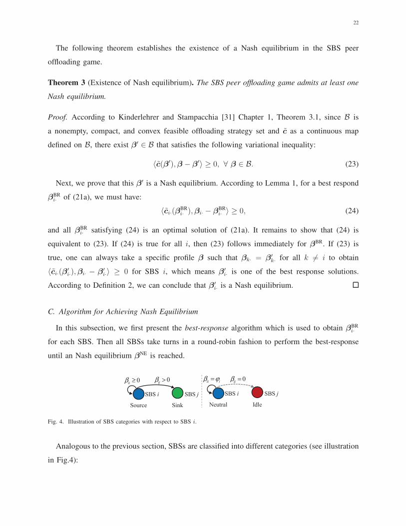
SinkSource

SBS i SBS j

0ii

β ≥ 0ijβ >

IdleNeutral

SBS i SBS j

ii iβ ϕ= 0ijβ =

Fig. 4. Illustration of SBS categories with respect to SBS i.

Analogous to the previous section, SBSs are classified into different categories (see illustration

in Fig.4):

23

• Source SBS (R). A SBS is a source SBS if it offloads a positive portion of its pre-offloading

workloads to other SBSs and processes the rest of workloads locally (0 ≤ βii < φi).

• Neutral SBS (U). A SBS is a neutral SBS if it processes all its pre-offloading workloads

locally (βii = φi).

• Idle SBS with respect to SBS i (Ii). A SBS is an idle SBS with respect to SBS i if it

does not receive any workload from SBS i (βij = 0).

• Sink SBS with respect to SBS i (Si). A SBS is a sink SBS with respect to SBS i if it

receives workload from SBS i (βij > 0).

The first two categories are defined depending on how the SBS handles its own pre-offloading

workloads. The last two categories are defined depending on how the SBS handles other SBSs’

workloads. Since there are N − 1 other SBSs, the categories are defined with respect to each

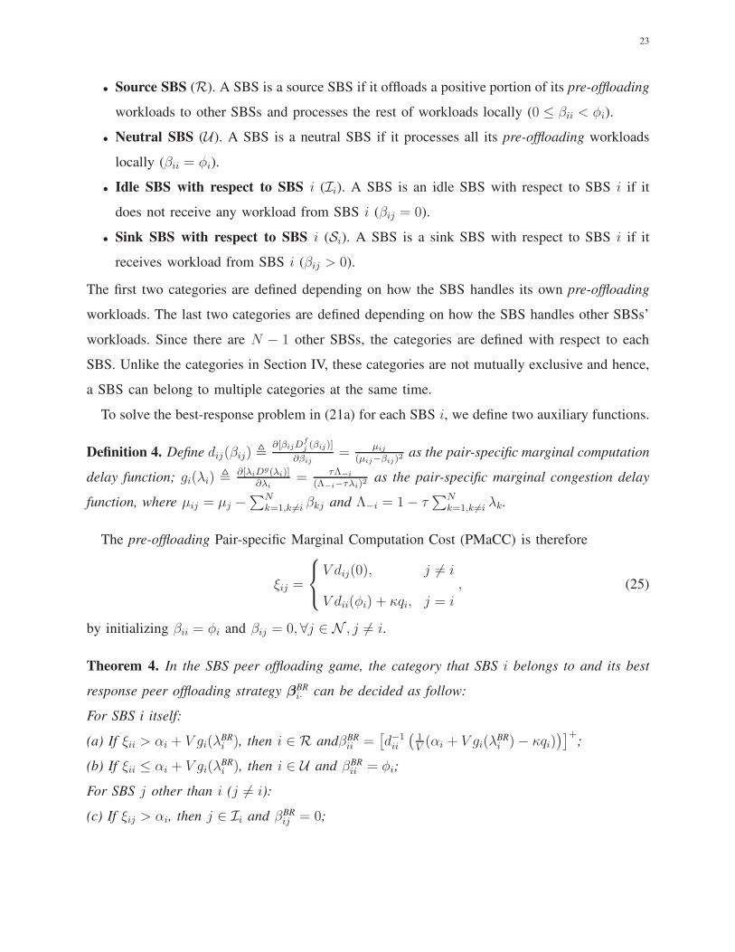
SBS. Unlike the categories in Section IV, these categories are not mutually exclusive and hence,

a SBS can belong to multiple categories at the same time.

To solve the best-response problem in (21a) for each SBS i, we define two auxiliary functions.

Definition 4. Define dij(βij) ,∂[βijD

fj (βij)]

∂βij=

µij

(µij−βij)2as the pair-specific marginal computation

delay function; gi(λi) ,∂[λiD

g(λi)]∂λi

= τΛ−i

(Λ−i−τλi)2as the pair-specific marginal congestion delay

function, where µij = µj −∑N

k=1,k 6=i βkj and Λ−i = 1− τ∑N

k=1,k 6=i λk.

The pre-offloading Pair-specific Marginal Computation Cost (PMaCC) is therefore

ξij =

V dij(0), j 6= i

V dii(φi) + κqi, j = i, (25)

by initializing βii = φi and βij = 0, ∀j ∈ N , j 6= i.

Theorem 4. In the SBS peer offloading game, the category that SBS i belongs to and its best

response peer offloading strategy βBRi· can be decided as follow:

For SBS i itself:

(a) If ξii > αi + V gi(λBRi ), then i ∈ R andβBR

ii =[d−1ii

(1V(αi + V gi(λ

BRi )− κqi)

)]+;

(b) If ξii ≤ αi + V gi(λBRi ), then i ∈ U and βBR

ii = φi;

For SBS j other than i (j 6= i):

(c) If ξij > αi, then j ∈ Ii and βBRij = 0;

24

(d) If ξij < αi, then j ∈ Si and βBRij = d−1

ij (αi

V);

where λBR, αi are the solution to workload flow equation

∑

j∈Si

d−1ij (

αi

V)

︸ ︷︷ ︸

λSi

: inbound workload to Si

= 1i ∈ R ·

(

φi − [d−1ij (

1

V(αi + V gi(λ

BRi )− qiκ))]

+

)

︸ ︷︷ ︸

λRi

: outbound workload from SBS i

.

Proof. See Appendix C in Supplementary File.

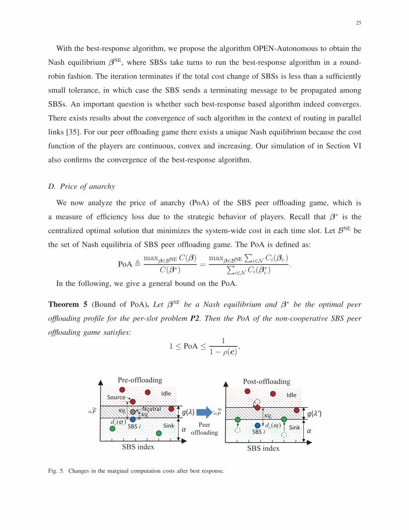
Theorem 4 can be explained in a similar way as Theorem 1. Figure 5 depicts the changes of

marginal computation costs when SBS i performs best response. One major difference is that

in the best-response algorithm, SBS i determines its sink SBSs by examining only the marginal

computation delay cost (i.e., dij), regardless of the marginal energy consumption cost (κqj) of

other SBSs. This is actually intuitive since each SBS aims to minimize its own cost rather

than the overall system cost. The solution for αi can be obtained by a binary search under the

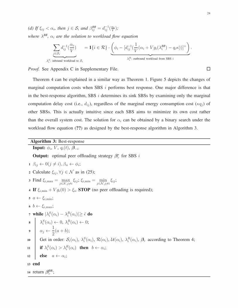
workload flow equation (??) as designed by the best-response algorithm in Algorithm 3.

Algorithm 3: Best-response

Input: φi, V , qi(t), β−i·

Output: optimal peer offloading strategy β∗i· for SBS i

1 βij ← 0(j 6= i), βii ← φi;

2 Calculate ξij, ∀j ∈ N as in (25);

3 Find ξi,max = maxj∈N ,j 6=i

ξij; ξi,min = minj∈N ,j 6=i

ξij;

4 If ξi,min + V gi(0) > ξii STOP (no peer offloading is required);

5 a← ξi,min;

6 b← ξi,max;

7 while |λSi (αi)− λRi (αi)|≥ ǫ do

8 λSi (αi)← 0, λRi (αi)← 0;

9 αj ←1

2(a+ b);

10 Get in order: Si(αi), λSi (αi), R(αi), U(αi), λ

Ri (αi), βi· according to Theorem 4;

11 if λSi (αi) > λRi (αi) then b← αi;

12 else a← αi;

13 end

14 return βBRi· ;

25

With the best-response algorithm, we propose the algorithm OPEN-Autonomous to obtain the

Nash equilibrium βNE, where SBSs take turns to run the best-response algorithm in a round-

robin fashion. The iteration terminates if the total cost change of SBSs is less than a sufficiently

small tolerance, in which case the SBS sends a terminating message to be propagated among

SBSs. An important question is whether such best-response based algorithm indeed converges.

There exists results about the convergence of such algorithm in the context of routing in parallel

links [35]. For our peer offloading game there exists a unique Nash equilibrium because the cost

function of the players are continuous, convex and increasing. Our simulation of in Section VI

also confirms the convergence of the best-response algorithm.

D. Price of anarchy

We now analyze the price of anarchy (PoA) of the SBS peer offloading game, which is

a measure of efficiency loss due to the strategic behavior of players. Recall that β∗ is the

centralized optimal solution that minimizes the system-wide cost in each time slot. Let BNE be

the set of Nash equilibria of SBS peer offloading game. The PoA is defined as:

PoA ,maxβ∈BNE C(β)

C(β∗)=

maxβ∈BNE

∑

i∈N Ci(βi·)∑

i∈N Ci(β∗i·)

.

In the following, we give a general bound on the PoA.

Theorem 5 (Bound of PoA). Let βNE be a Nash equilibrium and β∗ be the optimal peer

offloading profile for the per-slot problem P2. Then the PoA of the non-cooperative SBS peer

offloading game satisfies:

1 ≤ PoA ≤1

1− ρ(c),

ξ ij

SBS index

Pre-offloading

Peer

offloading

ξ'ij

i

iqκ ′iqκ

!"#$

!"#$%&

( )ii id ϕ

SBS index

Post-offloading

i

iqκ

( )ii id ω

Fig. 5. Changes in the marginal computation costs after best response.

26

where ρ(c) , supj∈N ρ(c·j), and

ρ(c·j) , supβ,β∈B

1∑N

i=1 βijcij(βi·)·

N∑

i=1

[

(cij(βi·)− cij(βi·))βij + (cij(βi·)− cij(βi·))βij

]

.

Proof. We rearrange system-wide cost C(βNE) as follows:

C(βNE)

=∑

i∈N

∑

j∈N

[(cij(β

NE)− cij(βNE))βNEij + cij(β

NE)βNEij

]

(†)

≤∑

i∈N

∑

j∈N

(cij(β

NE)− cij(βNE))βNEij +

∑

i∈N

∑

j∈N

cij(βNE)βij

(‡)

≤∑

j∈N

[

ρ(c·j)∑

i∈N

βNEij cij(β

NE)

]

+ C(β)

≤ ρ(c)C(βNE) + C(β).

where we use variational inequality (23) to get the inequality (†) and the definition of ρ(·) to

get the inequality (‡). We finish by taking β = β∗.

We further establish an upper bound on ρ(c·j), which is given by the following Lemma.

Lemma 2. Define δ(c·j) = supi,k∈N

c′ij(βi·)

c′kj(βk·)

and η(c·j) = supi,k∈N

ωjc′

ij(βi·)

ckj(βk·), ∀βi· ∈ Bi·, ∀βk· ∈

Bk·, where c′ij(βi·) =∂cij(βi·)

∂βij. If each cij is differentiable, nonnegative, increasing, and convex,

then the following inequality holds

ρ(c·j) ≤η(c·j)

3 +4

δ(c·j)(N − 1)

.

Proof. The proof follows Proposition 5.5 in [36].

According to Theorem 5 and Lemma 2, we see that the bound of PoA is mainly decided by

δ(c·j) = supi,k∈Nc′ij(βi·)

c′kj(βk·)

, i.e., the maximal ratio of SBSs’ pair-specific marginal cost values with

respect to SBS j. A larger δ(c·j) leads to a larger ρ(c·j), consequently, a larger PoA. The δ(c·j)

grows with the heterogeneity levels in task arrival rates and computation capacity among SBSs.

For example, suppose we have a SBS with an extremely large service rate, which gives a very

large δ(c·j). Then, all other SBSs tend to offload workload to that SBS, which causes a large

congestion delay in the LAN and hence increases the PoA value. Theoretically quantifying PoA

27

value is hard since it heavily depends on the task arrival pattern and system configuration. In

the simulation, we measure the PoA value in each time slot.

We have proved that for each time slot t the PoA of the peer offloading game is bounded.

Let max be the maximum achievable PoA across all time slots. Then, we have:

N∑

i=1

(V ·Dt

i(βNE,t) + qi(t) · E

ti (β

NE,t))≤ max

N∑

i=1

(V ·Dt

i(β∗,t) + qi(t) · E

ti (β

∗,t)). (26)

The strategic behavior of SBSs in the peer offloading game cause performance loss in both delay

and energy efficiency. The following theorem rigorously shows the performance guarantee of

OPEN-Autonomous.

Theorem 6. Following the peer offloading decision βNE,t obtained by OPEN-Autonomous, the

long-term system delay cost satisfies:

limT→∞

1

T

T−1∑

t=0

N∑

i=1

EDt

i(βNE,t)

≤ maxΨ(

max − 1

maxEmax) +

B

V,

and the long-term energy deficit of SBSs satisfies:

limT→∞

1

T

T−1∑

t=0

N∑

i=1

EEt

i (βNE,t)− Ei

≤B + V (maxDmax

sys −Doptsys)

maxǫ− (max − 1)Emax,

where max is the largest PoA value; Ψ(max−1max Emax) is the delay performance achieved by

stationary policy L satisfying energy consumption EEi(βL,t) − Ei ≤ −

max−1max Emax, where

Emax = maxi∈N Ei; ǫ > 0 is a constant which represents the long-term energy surplus achieved

by some stationary strategy.

Proof. See Appendix D in Supplementary File.

Theorem 6 still shows a [O(V ), O(1/V )] tradeoff between delay and energy deficit. However,

the delay performance achieved is no longer comparable with the optimal system delay Doptsys.

Instead, the bound of delay performance is defined on the stationary policies with a reduced

long-term energy constrain limT→∞1T

∑Tt=0 EEi(β

t) ≤ Emax/max. Notice that if max = 1,

then Theorem 6 is identical to Theorem 2.

VI. SIMULATION

Systematic simulations are carried out to evaluate the performance of proposed algorithm under

various system settings. We assume that the edge network is deployed in a commercial complex

28

where the business tenants deploy their own edge facilities (SBS and edge server) to serve their

employees. These SBSs are connected to a LAN and hence can cooperate with each other via

peer-offloading. The scale of the considered commercial complex should be large (>100,000

square feet [37]), such that multiple SBSs are likely to be deployed by different business

tenants and the collaboration among SBSs can be exploited. We simulated a 100m×100m

commercial complex (107,639 square feet) served by a set of SBSs whose locations are decided

by homogeneous Poisson Point Process (PPP). The main advantage of PPP is that it captures

the fact that SBSs are randomly deployed by individual owners. The density of PPP process is

set as 10−3. With this PPP density and commercial complex area, the expected number of SBSs

generated by PPP is 10 which is also the average number of business tenants in a commercial

complex within an area around 100,000 square feet [38]. Here, we assume that on average each

business tenant will deploy an SBS. In each time slot, the UEs are randomly scattered in the

network. Since the average working space of a worker is 250 square feet [39], the expected

number of users in the commercial complex is 400. Considering the variation in the occupancy

rate across the time, we assume that the number of UEs in each time slot is randomly drawn

from [200, 600]. Each UE is randomly assigned to one of its nearby SBSs. For an arbitrary

UE, its task generation follows a Poisson process with arrival rate πtm ∈ [0, 4]task/sec. The

expected number of CPU cycles for each task is h = 40M. The CPU frequency of edge server

at SBSs is fn = 3GHz. These parameters are picked to capture the fact that an edge server

can be overloaded from time to time. The expected input data size of each task is s = 0.2Mb.

Therefore, for a typical 100Mb fast Ethernet LAN, the expected transmission delay for one

task is τ = 200ms. The channel gain H tm for calculating the wireless transmission is modeled

by the indoor path-loss: L[dB] = 20 log(fTX[MHz]) + NL log(d[m]) − 28, where the values of

the parameters are listed in Table II. The wireless channel bandwidth is W = 20MHz, the

noise power is δ2 = −174dBm/Hz, the transmission power of UEs is P um = 10dBm. These

parameters are picked by following a typical wireless communication setting. Consider that the

energy consumption of one CPU cycles is 8.2nJ, the expected energy consumption for each

time at SBS n is κn = 9 × 10−5Wh and the long-term energy constraint is set as 22Wh per

hour. The performances of OPEN-Centralized (OPEN-C) and OPEN-Autonomous (OPEN-A)

are compared with three benchmarks:

• No Peer offloading (NoP): peer offloading among SBSs is not enabled in the network.

29

TABLE II

SIMULATION SETUP: SYSTEM PARAMETERS

Parameters Value

Expected number of SBSs, N 10 (Homogeneous PPP)

Expected number of UEs, M 400

Task arrival rate from UE m, πtm [0, 4]task/sec

Expected num. of CPU cycles per-task, h 40M

CPU frequency of edge server at SBS n, fn 3GHz

Expected input data size per-task, s 0.2Mb

Transmission delay for one task in LAN, τ 200ms

Wireless transmission frequency, fTX 900MHz

Distance power loss coefficient, NL 20

Wireless channel bandwidth, W 20MHz

Noise power, δ2 -174dBm/Hz

Transmission power of UEs, Pum 10dBm

Expected energy consumption per-task, κn 9× 10−5W·h

Long-term energy constraint, En 22W·h (per hour)

Each SBS processes all the tasks received from the end users. Moreover, the long-term

constraint is not enforced since some SBSs have to exceed energy constraint to satisfy all

the tasks due to the heterogeneity in spatial task arrival.

• Delay-Optimal (D-Optimal): we apply the method in [40] where SBS peer offloading is

considered as a static load balancing problem aiming to achieve the lowest system delay

regardless of the long-term energy constraints.

• Single-Slot Constraint (SSC): Instead of following a long-term energy constraint, the

network operator poses a hard energy constraint in each time slot, i.e. Eti (β

t) ≤ Ei, such

that the long-term energy constraint is satisfied.

A. Run-time Performance Evaluation

Figure 6 shows the long-term system performance obtained by running OPEN and we mainly

focus on two metrics: the time-average system delay cost in Figure 6(a) and the time-average

energy deficit in Figure 6(b). It can be observed that without peer offloading the edge system

bears a high delay cost and a large energy deficit, since SBSs can be easily overloaded due to

30

100 200 300 400 500 600

Time slot t

0

50

100

150

Tim

e-av

erag

e sy

stem

del

ay

OPEN-COPEN-ANoPD-optimalSSC

(a) Time average system delay.

100 200 300 400 500 600

Time slot t

0

10

20

30

40

50

Tim

e-av

erag

e en

ergy

def

icit OPEN-C

OPEN-ANoPD-optimalSSC

(b) Time average energy deficit.

Fig. 6. Long-term performance analysis.

spatially and temporally heterogeneous task arrival pattern. By contrast, other three schemes with

peer offloading enabled (D-Optimal, SSC, and OPEN) achieve much lower system delay cost.

Specifically, D-Optimal achieves the lowest delay cost since it is designed to minimize the delay

cost by fully utilizing the computation resource regardless of the energy constraints. Therefore,

D-Optimal incurs a large amount of energy deficit as shown in Figure 6(b). The main purpose

of OPEN is to follow the long-term energy constraint of each SBS while minimizing the system

delay. As can be observed in Figure 6(b), the time-average energy deficits of both OPEN-C and

OPEN-A coverage to zero, which means that the long-term energy constraints are satisfied by

running OPEN. Moreover, OPEN-C achieves a close-to-optimal delay cost and OPEN-A incurs

a slightly higher delay cost due to the strategic behaviors of selfish SBSs. The SSC scheme

poses an energy constraint in each time slot in order to satisfy the long-term energy constraints.

As a result, the energy deficit of SSC is zero across all the time slots. However, SSC makes the

energy scheduling less flexible and therefore does not handle well the heterogeneity of temporal

task arrival pattern and results in a large system delay cost.

B. System Dynamics

Figure 7 and Figure 8 show the system delay cost and the energy consumption from the 500th

to 550th time slot, respectively. We see that the system delay cost is mainly decided by the total

task arrival rate in the network which varies across the time slots. Usually, a larger task arrival

rate will result in a higher system delay cost. Figure 8 depicts the energy consumption of one

particular SBS and the corresponding energy deficit queue in each time slot to exemplify how

the energy deficit queue works to guide the energy usage. For example, from the 530th to 535th

31

time slot, the SBS uses a large amount of energy and enlarges the energy deficit. Therefore, in

the following 5 time slots, OPEN reduces the energy consumption to cut the energy deficit. In

this way, the long-term energy constraints of SBSs can be satisfied.

500 510 520 530 540 550Time slots

0

50

100

150

200

250

Sys

tem

del

ay c

ost

0

30

60

90

120

150

Tot

al ta

sk a

rriv

al

System delay costTotal task arrival

Fig. 7. System dynamics (delay cost).

500 510 520 530 540 550Time slots

0

20

40

60

80

100

120

140

Ene

rgy

cons

umpt

ion

100

150

200

250

300

Ene

rgy

defic

it qu

eue

Energy consumptionEnergy deficit queue

Fig. 8. System dynamics (energy consumption).

C. Impact of Control Parameter V

Figure 9 shows the impact of control parameter V on the performance of OPEN. The result

presents a [O(1/V ), O(V )] trade-off between the long-term system delay cost and the long-

term energy deficit, which is consistent with our theoretical analysis. With a larger V , OPEN

emphasizes more on the system delay cost and is less concerned with the energy deficit. As V

grows to the infinity, OPEN is able to achieve the optimal delay cost. It is hard to define an

optimal value for V since a lower system delay cost is achieved at the cost of larger energy deficit.

However, it still offers a guideline for picking an appropriate V . In this particular simulation, the

network operator is recommended to choose, for example, V = 50 for two reasons: (i) OPEN

has already achieved close-to-optimal delay and little improvement is available by increasing

V ; (ii) the energy deficit is much smaller compared to the energy deficit achieving the optimal

delay.

D. Composition of System Delay

Figure 10 and Figure 11 depict the composition of system delay cost for OPEN-C and OPEN-

A, receptively. For OPEN-C, the computation delay cost takes up a large proportion of the system

delay cost and the congestion delay cost is relatively small. By contrast, the congestion delay cost

becomes the main part of the system delay cost in OPEN-A. The non-cooperative behavior of

32

0 50 100 150Control parameter V

30

60

90

120

150

Long

-ter

m s

yste

m d

elay

0

1

2

3

4

Long

-ter

m e

nerg

y de

ficitTime-average system delay

Time-average energy deficit

Optimal system delay

Fig. 9. Impact of control parameter V .

SBSs results in a large volume of traffic exchange in the LAN as SBSs tend to offload workload

to other SBSs in order to save their own energy consumption. Note that the communication

delay cost is independent of peer offloading and hence it is the same for OPEN-C and OPEN-A.

0 100 200 300 400 500 600

Time slot t

0

10

20

30

40

50

60

70

80

Tim

e-av

erag

e sy

stem

del

ay

Computation delay

Congestion delay Communication delay

Fig. 10. Delay cost composition of OPEN-C.

0 100 200 300 400 500 600

Time slot t

0

10

20

30

40

50

60

70

80

Tim

e-av

erag

e sy

stem

del

ay

Congestion delay

Computation delay

Communication delay

Fig. 11. Delay cost composition of OPEN-A.

E. Price of Anarchy

Since it is difficult to quantify theoretically the upper bound of PoA, we measure PoA values

in the simulation. Figure 12 depicts the objective value (P2) achieved by OPEN-C and OPEN-A

from the 50th time slot to the 100th time slot from a simulation run of a total of 600 time

slots. It is clearly shown that in each time slot OPEN-C achieves a strictly smaller value than

OPEN-A, which means that OPEN-C outperforms OPEN-A in every time slot. For the entire

600 time slots, the mean PoA value is 1.54 and the maximum PoA value is 2.42.

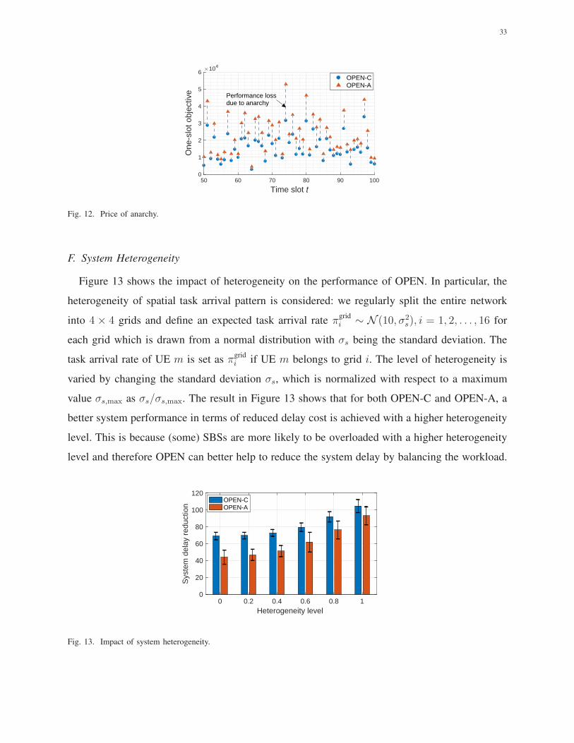
33

50 60 70 80 90 100

Time slot t

0

1

2

3

4

5

6

One

-slo

t obj

ectiv

e

104

OPEN-COPEN-A

Performance lossdue to anarchy

Fig. 12. Price of anarchy.

F. System Heterogeneity

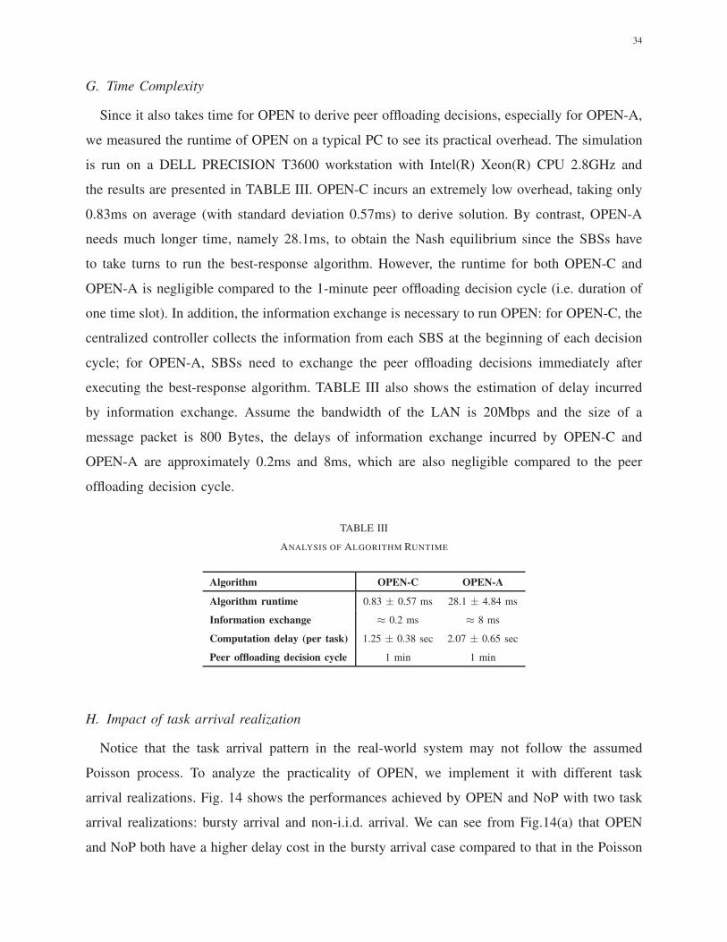
Figure 13 shows the impact of heterogeneity on the performance of OPEN. In particular, the

heterogeneity of spatial task arrival pattern is considered: we regularly split the entire network

into 4 × 4 grids and define an expected task arrival rate πgridi ∼ N (10, σ2

s), i = 1, 2, . . . , 16 for

each grid which is drawn from a normal distribution with σs being the standard deviation. The

task arrival rate of UE m is set as πgridi if UE m belongs to grid i. The level of heterogeneity is

varied by changing the standard deviation σs, which is normalized with respect to a maximum

value σs,max as σs/σs,max. The result in Figure 13 shows that for both OPEN-C and OPEN-A, a

better system performance in terms of reduced delay cost is achieved with a higher heterogeneity

level. This is because (some) SBSs are more likely to be overloaded with a higher heterogeneity

level and therefore OPEN can better help to reduce the system delay by balancing the workload.

0 0.2 0.4 0.6 0.8 1Heterogeneity level

0

20

40

60

80

100

120

Sys

tem

del

ay r

educ

tion

OPEN-COPEN-A

Fig. 13. Impact of system heterogeneity.

34

G. Time Complexity

Since it also takes time for OPEN to derive peer offloading decisions, especially for OPEN-A,

we measured the runtime of OPEN on a typical PC to see its practical overhead. The simulation

is run on a DELL PRECISION T3600 workstation with Intel(R) Xeon(R) CPU 2.8GHz and

the results are presented in TABLE III. OPEN-C incurs an extremely low overhead, taking only

0.83ms on average (with standard deviation 0.57ms) to derive solution. By contrast, OPEN-A

needs much longer time, namely 28.1ms, to obtain the Nash equilibrium since the SBSs have

to take turns to run the best-response algorithm. However, the runtime for both OPEN-C and

OPEN-A is negligible compared to the 1-minute peer offloading decision cycle (i.e. duration of

one time slot). In addition, the information exchange is necessary to run OPEN: for OPEN-C, the

centralized controller collects the information from each SBS at the beginning of each decision

cycle; for OPEN-A, SBSs need to exchange the peer offloading decisions immediately after

executing the best-response algorithm. TABLE III also shows the estimation of delay incurred

by information exchange. Assume the bandwidth of the LAN is 20Mbps and the size of a

message packet is 800 Bytes, the delays of information exchange incurred by OPEN-C and

OPEN-A are approximately 0.2ms and 8ms, which are also negligible compared to the peer

offloading decision cycle.

TABLE III

ANALYSIS OF ALGORITHM RUNTIME

Algorithm OPEN-C OPEN-A

Algorithm runtime 0.83 ± 0.57 ms 28.1 ± 4.84 ms

Information exchange ≈ 0.2 ms ≈ 8 ms

Computation delay (per task) 1.25 ± 0.38 sec 2.07 ± 0.65 sec

Peer offloading decision cycle 1 min 1 min

H. Impact of task arrival realization

Notice that the task arrival pattern in the real-world system may not follow the assumed

Poisson process. To analyze the practicality of OPEN, we implement it with different task

arrival realizations. Fig. 14 shows the performances achieved by OPEN and NoP with two task

arrival realizations: bursty arrival and non-i.i.d. arrival. We can see from Fig.14(a) that OPEN

and NoP both have a higher delay cost in the bursty arrival case compared to that in the Poisson

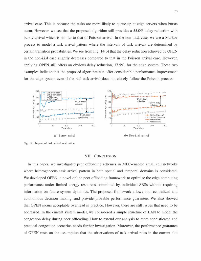
35

arrival case. This is because the tasks are more likely to queue up at edge servers when bursts

occur. However, we see that the proposed algorithm still provides a 55.0% delay reduction with

bursty arrival which is similar to that of Poisson arrival. In the non-i.i.d. case, we use a Markov

process to model a task arrival pattern where the intervals of task arrivals are determined by

certain transition probabilities. We see from Fig. 14(b) that the delay reduction achieved by OPEN

in the non-i.i.d case slightly decreases compared to that in the Poisson arrival case. However,

applying OPEN still offers an obvious delay reduction, 37.5%, for the edge system. These two

examples indicate that the proposed algorithm can offer considerable performance improvement

for the edge system even if the real task arrival does not closely follow the Poisson process.

0 50 100 150 200Time slots

0

50

100

150

200

250

Tim

e-av

erag

e de

lay

cost

OPEN-C(Bursty)OPEN-C(Poisson)NoP(Bursty)NoP(Poisson)

55.0% delayreduction

54.5% delayreduction

(a) Bursty arrival

0 50 100 150 200Time slots

0

20

40

60

80

100

120

Tim

e-av

erag

e de

lay

cost

OPEN-C(Non-iid)OPEN-C(Poisson)NoP(Non-iid)NoP(Poisson)

54.5% delayreduction

37.5% delayreduction

(b) Non-i.i.d. arrival

Fig. 14. Impact of task arrival realization.

VII. CONCLUSION

In this paper, we investigated peer offloading schemes in MEC-enabled small cell networks

where heterogeneous task arrival pattern in both spatial and temporal domains is considered.

We developed OPEN, a novel online peer offloading framework to optimize the edge computing

performance under limited energy resources committed by individual SBSs without requiring

information on future system dynamics. The proposed framework allows both centralized and

autonomous decision making, and provide provable performance guarantee. We also showed

that OPEN incurs acceptable overhead in practice. However, there are still issues that need to be

addressed. In the current system model, we considered a simple structure of LAN to model the

congestion delay during peer offloading. How to extend our analysis to more sophisticated and

practical congestion scenarios needs further investigation. Moreover, the performance guarantee

of OPEN rests on the assumption that the observations of task arrival rates in the current slot

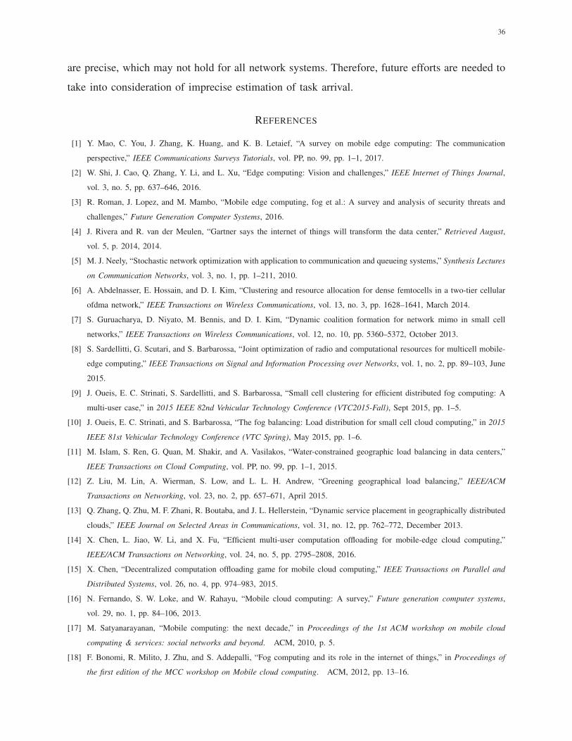
36

are precise, which may not hold for all network systems. Therefore, future efforts are needed to

take into consideration of imprecise estimation of task arrival.

REFERENCES

[1] Y. Mao, C. You, J. Zhang, K. Huang, and K. B. Letaief, “A survey on mobile edge computing: The communication

perspective,” IEEE Communications Surveys Tutorials, vol. PP, no. 99, pp. 1–1, 2017.

[2] W. Shi, J. Cao, Q. Zhang, Y. Li, and L. Xu, “Edge computing: Vision and challenges,” IEEE Internet of Things Journal,

vol. 3, no. 5, pp. 637–646, 2016.

[3] R. Roman, J. Lopez, and M. Mambo, “Mobile edge computing, fog et al.: A survey and analysis of security threats and

challenges,” Future Generation Computer Systems, 2016.

[4] J. Rivera and R. van der Meulen, “Gartner says the internet of things will transform the data center,” Retrieved August,

vol. 5, p. 2014, 2014.

[5] M. J. Neely, “Stochastic network optimization with application to communication and queueing systems,” Synthesis Lectures

on Communication Networks, vol. 3, no. 1, pp. 1–211, 2010.

[6] A. Abdelnasser, E. Hossain, and D. I. Kim, “Clustering and resource allocation for dense femtocells in a two-tier cellular

ofdma network,” IEEE Transactions on Wireless Communications, vol. 13, no. 3, pp. 1628–1641, March 2014.

[7] S. Guruacharya, D. Niyato, M. Bennis, and D. I. Kim, “Dynamic coalition formation for network mimo in small cell

networks,” IEEE Transactions on Wireless Communications, vol. 12, no. 10, pp. 5360–5372, October 2013.

[8] S. Sardellitti, G. Scutari, and S. Barbarossa, “Joint optimization of radio and computational resources for multicell mobile-

edge computing,” IEEE Transactions on Signal and Information Processing over Networks, vol. 1, no. 2, pp. 89–103, June

2015.

[9] J. Oueis, E. C. Strinati, S. Sardellitti, and S. Barbarossa, “Small cell clustering for efficient distributed fog computing: A

multi-user case,” in 2015 IEEE 82nd Vehicular Technology Conference (VTC2015-Fall), Sept 2015, pp. 1–5.

[10] J. Oueis, E. C. Strinati, and S. Barbarossa, “The fog balancing: Load distribution for small cell cloud computing,” in 2015

IEEE 81st Vehicular Technology Conference (VTC Spring), May 2015, pp. 1–6.

[11] M. Islam, S. Ren, G. Quan, M. Shakir, and A. Vasilakos, “Water-constrained geographic load balancing in data centers,”

IEEE Transactions on Cloud Computing, vol. PP, no. 99, pp. 1–1, 2015.

[12] Z. Liu, M. Lin, A. Wierman, S. Low, and L. L. H. Andrew, “Greening geographical load balancing,” IEEE/ACM

Transactions on Networking, vol. 23, no. 2, pp. 657–671, April 2015.

[13] Q. Zhang, Q. Zhu, M. F. Zhani, R. Boutaba, and J. L. Hellerstein, “Dynamic service placement in geographically distributed

clouds,” IEEE Journal on Selected Areas in Communications, vol. 31, no. 12, pp. 762–772, December 2013.

[14] X. Chen, L. Jiao, W. Li, and X. Fu, “Efficient multi-user computation offloading for mobile-edge cloud computing,”

IEEE/ACM Transactions on Networking, vol. 24, no. 5, pp. 2795–2808, 2016.

[15] X. Chen, “Decentralized computation offloading game for mobile cloud computing,” IEEE Transactions on Parallel and

Distributed Systems, vol. 26, no. 4, pp. 974–983, 2015.

[16] N. Fernando, S. W. Loke, and W. Rahayu, “Mobile cloud computing: A survey,” Future generation computer systems,

vol. 29, no. 1, pp. 84–106, 2013.

[17] M. Satyanarayanan, “Mobile computing: the next decade,” in Proceedings of the 1st ACM workshop on mobile cloud

computing & services: social networks and beyond. ACM, 2010, p. 5.

[18] F. Bonomi, R. Milito, J. Zhu, and S. Addepalli, “Fog computing and its role in the internet of things,” in Proceedings of

the first edition of the MCC workshop on Mobile cloud computing. ACM, 2012, pp. 13–16.

37

[19] M. Satyanarayanan, P. Bahl, R. Caceres, and N. Davies, “The case for vm-based cloudlets in mobile computing,” IEEE

pervasive Computing, vol. 8, no. 4, 2009.

[20] A. Greenberg, J. Hamilton, D. A. Maltz, and P. Patel, “The cost of a cloud: research problems in data center networks,”

ACM SIGCOMM computer communication review, vol. 39, no. 1, pp. 68–73, 2008.

[21] TROPIC. (2015) Distributed computing storage and radio resource allocation over cooperative femtocells. [Online].

Available: http://www.ict-tropic.eu.

[22] J. Rubio, A. Pascual-Iserte, J. del Olmo, and J. Vidal, “User association for load balancing in heterogeneous networks

powered with energy harvesting sources,” in 2014 IEEE Globecom Workshops (GC Wkshps), Dec 2014, pp. 1248–1253.

[23] H. H. M. Tam, H. D. Tuan, D. T. Ngo, T. Q. Duong, and H. V. Poor, “Joint load balancing and interference management

for small-cell heterogeneous networks with limited backhaul capacity,” IEEE Transactions on Wireless Communications,

vol. 16, no. 2, pp. 872–884, Feb 2017.

[24] M. Lin, Z. Liu, A. Wierman, and L. L. Andrew, “Online algorithms for geographical load balancing,” in Green Computing

Conference (IGCC), 2012 International. IEEE, 2012, pp. 1–10.

[25] H. Xu, C. Feng, and B. Li, “Temperature aware workload managementin geo-distributed data centers,” IEEE Transactions

on Parallel and Distributed Systems, vol. 26, no. 6, pp. 1743–1753, 2015.

[26] J. Luo, L. Rao, and X. Liu, “Spatio-temporal load balancing for energy cost optimization in distributed internet data

centers,” IEEE Transactions on Cloud Computing, vol. 3, no. 3, pp. 387–397, July 2015.

[27] Z. Liu, M. Lin, A. Wierman, S. H. Low, and L. L. Andrew, “Greening geographical load balancing,” in Proceedings of

the ACM SIGMETRICS joint international conference on Measurement and modeling of computer systems. ACM, 2011,

pp. 233–244.

[28] F. Farahnakian, P. Liljeberg, and J. Plosila, “Energy-efficient virtual machines consolidation in cloud data centers using

reinforcement learning,” in Parallel, Distributed and Network-Based Processing (PDP), 2014 22nd Euromicro International

Conference on. IEEE, 2014, pp. 500–507.

[29] X. Zhou, K. Wang, W. Jia, and M. Guo, “Reinforcement learning-based adaptive resource management of differentiated

services in geo-distributed data centers,” in Quality of Service (IWQoS), 2017 IEEE/ACM 25th International Symposium

on. IEEE, 2017, pp. 1–6.

[30] N. Nisan, T. Roughgarden, E. Tardos, and V. V. Vazirani, Algorithmic game theory. Cambridge University Press Cambridge,

2007, vol. 1.

[31] D. Kinderlehrer and G. Stampacchia, An introduction to variational inequalities and their applications. SIAM, 2000.

[32] R. B. Cooper, Introduction to queueing theory. North Holland, 1981.

[33] C. H. Liu, P. Hui, J. W. Branch, C. Bisdikian, and B. Yang, “Efficient network management for context-aware participatory

sensing,” in Sensor, mesh and ad hoc commun. and networks, 2011 8th annual IEEE Conf. on. IEEE, 2011, pp. 116–124.

[34] M. Mihailescu and Y. M. Teo, “On economic and computational-efficient resource pricing in large distributed systems,”

in 2010 10th IEEE/ACM International Conference on Cluster, Cloud and Grid Computing, May 2010, pp. 838–843.

[35] Y. A. Korilis, A. A. Lazar, and A. Orda, “Capacity allocation under noncooperative routing,” IEEE Transactions on

Automatic Control, vol. 42, no. 3, pp. 309–325, Mar 1997.

[36] C. Durr, “Congestion games with player-specific cost functions,” Ph.D. dissertation, Universite Paris-Est, 2014.

[37] S. Katipamula, R. M. Underhill, J. K. Goddard, D. J. Taasevigen, M. Piette, J. Granderson, R. E. Brown, S. M. Lanzisera,

and T. Kuruganti, “Small-and medium-sized commercial building monitoring and controls needs: A scoping study,” Pacific

Northwest National Lab.(PNNL), Richland, WA (United States), Tech. Rep., 2012.

[38] IREM, “Trends in office buildings operations,” Institute of Real Estate Management, Tech. Rep., 2012.

38

[39] Gridium. (2015) Density trends in commercial real estate. [Online]. Available:

https://gridium.com/imagine-your-building-with-35-more-people-in-it/

[40] S. Penmatsa and A. T. Chronopoulos, “Game-theoretic static load balancing for distributed systems,” Journal of Parallel

and Distributed Computing, vol. 71, no. 4, pp. 537–555, 2011.

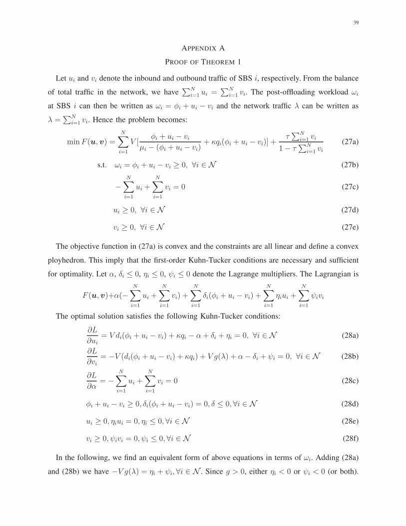
39

APPENDIX A

PROOF OF THEOREM 1

Let ui and vi denote the inbound and outbound traffic of SBS i, respectively. From the balance

of total traffic in the network, we have∑N

i=1 ui =∑N

i=1 vi. The post-offloading workload ωi

at SBS i can then be written as ωi = φi + ui − vi and the network traffic λ can be written as

λ =∑N

i=1 vi. Hence the problem becomes:

minF (u, v) =

N∑

i=1

V [φi + ui − vi

µi − (φi + ui − vi)+ κqi(φi + ui − vi)] +

τ∑N

i=1 vi

1− τ∑N

i=1 vi(27a)

s.t. ωi = φi + ui − vi ≥ 0, ∀i ∈ N (27b)

−N∑

i=1

ui +N∑

i=1

vi = 0 (27c)

ui ≥ 0, ∀i ∈ N (27d)

vi ≥ 0, ∀i ∈ N (27e)

The objective function in (27a) is convex and the constraints are all linear and define a convex

ployhedron. This imply that the first-order Kuhn-Tucker conditions are necessary and sufficient

for optimality. Let α, δi ≤ 0, ηi ≤ 0, ψi ≤ 0 denote the Lagrange multipliers. The Lagrangian is

F (u, v)+α(−N∑

i=1

ui +N∑

i=1

vi) +N∑

i=1

δi(φi + ui − vi) +N∑

i=1

ηiui +N∑

i=1

ψivi

The optimal solution satisfies the following Kuhn-Tucker conditions:

∂L

∂ui= V di(φi + ui − vi) + κqi − α+ δi + ηi = 0, ∀i ∈ N (28a)

∂L

∂vi= −V (di(φi + ui − vi) + κqi) + V g(λ) + α− δi + ψi = 0, ∀i ∈ N (28b)

∂L

∂α= −

N∑

i=1

ui +N∑

i=1

vi = 0 (28c)

φi + ui − vi ≥ 0, δi(φi + ui − vi) = 0, δ ≤ 0, ∀i ∈ N (28d)

ui ≥ 0, ηiui = 0, ηi ≤ 0, ∀i ∈ N (28e)

vi ≥ 0, ψivi = 0, ψi ≤ 0, ∀i ∈ N (28f)

In the following, we find an equivalent form of above equations in terms of ωi. Adding (28a)

and (28b) we have −V g(λ) = ηi + ψi, ∀i ∈ N . Since g > 0, either ηi < 0 or ψi < 0 (or both).

40

Hence, from (28e) and (28f), for each i, either ui = 0 or vi = 0 (or both). We consider each

case separately.

• Case I: ui = 0, vi = 0, then we have ωi = φi. It follows from (28d) that δi = 0. Substituting

this into (28a) and (28b) gives

V di(ωi) + κqi = α− ηi ≥ α

V di(ωi) + κqi = V g(λ) + α + ψi < α + g(λ)

From the above, we have

α ≤ V di(ωi) + κqi ≤ α + V g(λ) (29)

This case corresponds to the neutral SBS.

• Case II: ui = 0, vi > 0. This case corresponds to source SBS. From (28f) we have ψi = 0 and

consider the following two subcases:

– Case II.1: vi < φi. Then, we have 0 < ωi < φi. It follows from (28d) that δi = 0. Substituting

this in to (28a),(28b) gives

V di(ωi) + κqi = α− ηi ≥ α (30)

V di(ωi) + κqi = α + V g(λ) (31)

– Case II.2: vi = φi. Then, we have ωi = 0 and (28a), (28b) gives

V di(ωi) + κqi = α− δi − ηi ≥ α

V di(ωi) + κqi = α + V g(λ)− δi ≥ α+ g(λ).

Thus, we have V di(ωi) + κqi ≥ α + V g(λ).

• Case III: ui > 0, vi = 0. Then, we have ωi > φi. It follows from (28d) and (28e) that δi = 0

and ηi = 0. Substituting this in to (28a), we have

V di(ωi) + κqi = α. (32)

This case corresponds to sink SBS.

Using (31) and (32), we have the total flow constraint:

∑

i∈S

(d−1i

(1

V(α− κqi)

)

− φi) =∑

i∈R

(φi − [d−1i

(1

V(α + V g(λ)− κqi)

)

]+)

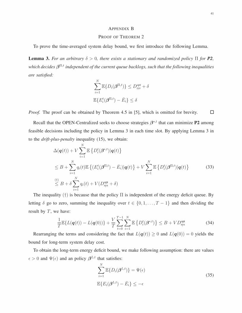
41

APPENDIX B

PROOF OF THEOREM 2

To prove the time-averaged system delay bound, we first introduce the following Lemma.

Lemma 3. For an arbitrary δ > 0, there exists a stationary and randomized policy Π for P2,

which decides βΠ,t independent of the current queue backlogs, such that the following inequalities

are satisfied:

N∑

i=1

EDi(βΠ,t) ≤ Dopt

sys + δ

EEti (β

Π,t)− Ei ≤ δ

Proof. The proof can be obtained by Theorem 4.5 in [5], which is omitted for brevity.

Recall that the OPEN-Centralized seeks to choose strategies β∗,t that can minimize P2 among

feasible decisions including the policy in Lemma 3 in each time slot. By applying Lemma 3 in

to the drift-plus-penalty inequality (15), we obtain:

∆(q(t)) + V

N∑

i=1

EDt

i(β∗,t)|q(t)

≤ B +N∑

i=1

qi(t)E(Et

i (βΠ,t)− Ei)|q(t)

+ V

N∑

i=1

EDt

i(βΠ,t)|q(t)

(†)

≤ B + δ

N∑

i=1

qi(t) + V (Doptsys + δ)

(33)

The inequality (†) is because that the policy Π is independent of the energy deficit queue. By

letting δ go to zero, summing the inequality over t ∈ 0, 1, . . . , T − 1 and then dividing the

result by T , we have:

1

TEL(q(t))− L(q(0))+

V

T

T−1∑

t=0

N∑

i=1

EDt

i(β∗,t)≤ B + V Dopt

sys (34)

Rearranging the terms and considering the fact that L(q(t)) ≥ 0 and L(q(0)) = 0 yields the

bound for long-term system delay cost.

To obtain the long-term energy deficit bound, we make following assumption: there are values

ǫ > 0 and Ψ(ǫ) and an policy βL,t that satisfies:

N∑

i=1

EDi(βL,t) = Ψ(ǫ)

EEi(βL,t)− Ei ≤ −ǫ

(35)

42

Plugging above into inequality (15)

∆(q(t)) + VN∑

i=1

EDt

i(β∗,t)≤ B + VΨ(ǫ)− ǫ

N∑

i=1

qi(t)

Summing the above over t ∈ 0, 1, . . . , T − 1 and rearranging terms as usual yields:

1

T

T−1∑

t=0

N∑

i=1

Eqi(t)

≤

B + V (Ψ(ǫ)−1

T

T−1∑

t=0

N∑

i=1

E Dti(β

∗,t)

ǫ

≤B + V (Dmax

sys −Doptsys)

ǫ

(36)

ConsideringT−1∑

t=0

N∑

i=1

Eqi(t) ≥T−1∑

t=0

N∑

i=1

EEi(βt)−Ei yields the long-term energy deficit bound.

APPENDIX C

PROOF OF THEOREM 4

Proof. We first restate the problem introducing the variables uij and vij , where uij denotes SBS

i’s workloads into SBS j and vij denotes SBS i’s workloads out of SBS j. Given our system

model, we only have vij 6= 0 when i = j.

From the balance of the of the total traffic of SBS i in the network, we have λi =∑N

j=1 uij =

vii. The workload βij offloaded from SBS i to SBS j can be written as

βij =

uij, if j 6= i

φi − vii, if j = i(37)

which can be rewritten as:

βij = φij + uij − vij where φij =

φi, if j = i

0, if j 6= i(38)

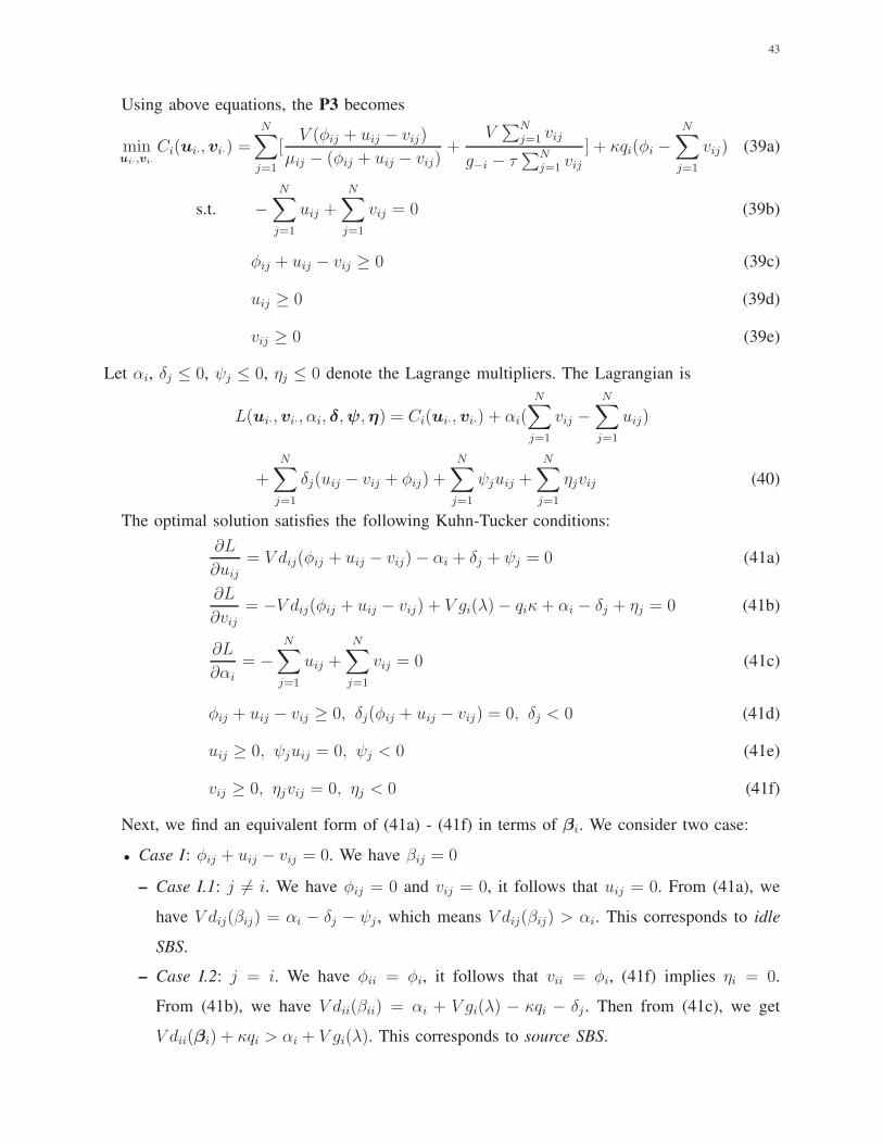
43

Using above equations, the P3 becomes

minui·,vi·

Ci(ui·, vi·) =N∑

j=1

[V (φij + uij − vij)

µij − (φij + uij − vij)+

V∑N

j=1 vij

g−i − τ∑N

j=1 vij] + κqi(φi −

N∑

j=1

vij) (39a)

s.t. −N∑

j=1

uij +

N∑

j=1

vij = 0 (39b)

φij + uij − vij ≥ 0 (39c)

uij ≥ 0 (39d)

vij ≥ 0 (39e)

Let αi, δj ≤ 0, ψj ≤ 0, ηj ≤ 0 denote the Lagrange multipliers. The Lagrangian is

L(ui·, vi·, αi, δ,ψ,η) = Ci(ui·, vi·) + αi(N∑

j=1

vij −N∑

j=1

uij)

+N∑

j=1

δj(uij − vij + φij) +N∑

j=1

ψjuij +N∑

j=1

ηjvij (40)

The optimal solution satisfies the following Kuhn-Tucker conditions:

∂L

∂uij= V dij(φij + uij − vij)− αi + δj + ψj = 0 (41a)

∂L

∂vij= −V dij(φij + uij − vij) + V gi(λ)− qiκ+ αi − δj + ηj = 0 (41b)

∂L

∂αi

= −N∑

j=1

uij +

N∑

j=1

vij = 0 (41c)

φij + uij − vij ≥ 0, δj(φij + uij − vij) = 0, δj < 0 (41d)

uij ≥ 0, ψjuij = 0, ψj < 0 (41e)

vij ≥ 0, ηjvij = 0, ηj < 0 (41f)

Next, we find an equivalent form of (41a) - (41f) in terms of βi. We consider two case:

• Case I: φij + uij − vij = 0. We have βij = 0

– Case I.1: j 6= i. We have φij = 0 and vij = 0, it follows that uij = 0. From (41a), we

have V dij(βij) = αi − δj − ψj , which means V dij(βij) > αi. This corresponds to idle

SBS.

– Case I.2: j = i. We have φii = φi, it follows that vii = φi, (41f) implies ηi = 0.

From (41b), we have V dii(βii) = αi + V gi(λ) − κqi − δj . Then from (41c), we get

V dii(βi) + κqi > αi + V gi(λ). This corresponds to source SBS.

44

• Case II: φij + uij − vij > 0. From (41c), we have δj = 0

– Case II.1: vij > 0, we must have j = i. From (41f), we have ηj = 0. (41b) implies

V dii(βii) + κqi = αi + V gi(λ). This case corresponds to source SBS.

– Case II.2: vij = 0.

∗ Case II.2.1: uij = 0. For i 6= j, it is equivalent to Case I.1. We consider j = i. Then

βii = φi. From (41b) and (41e), we have V dii(βii) + κqi < αi + V gi(λ). This case

corresponds to the neutral SBS.

∗ Case II.2.2: uij > 0, we must have j 6= i. Then βij > φij = 0. From (41e), we have

ψj = 0. Substituting this in (41a), we have V dij(βij) = αi. This case corresponds to

sink SBS for SBS i.

Equation (41c) may be written in terms of βij as

∑

j∈Si

d−1ij (

αi

V) =

∑

i∈R

(

φi − [d−1ij (

1

V(αi + V gi(λ)− qiκ))]

+

)

where αi is the Lagrange multiplier.

APPENDIX D

PROOF OF THEOREM 6

The proof of Theorem 6 is similar to that of Theorem 2. We reuse the assumption in (35).

Given the drift-plus-cost bound in (15) and the PoA bound in (26), we have

∆(q(t)) + VN∑

i=1

EDt

i(βNE,t)|q(t)

≤ B +

N∑

i=1

qi(t)E(Et

i (βNE,t)− Ei)|q(t)

+ V

N∑

i=1

EDt

i(βNE,t)|q(t)

≤ B +N∑

i=1

qi(t)E(maxEt

i (β∗,t)− Ei)|q(t)

+ maxV

N∑

i=1

EDt

i(β∗,t)|q(t)

≤ B +

N∑

i=1

qi(t)E(maxEt

i (βL,t)− maxEi)|q(t)

+

N∑

i=1

qi(t)E(max − 1)Ei)|q(t)

+ maxVN∑

i=1

EDt

i(βL,t)|q(t)

≤ B +((max − 1)Emax − maxǫ

)N∑

i=1

qi(t) + maxVΨ(ǫ)

45

Letting ǫ = max−1max Emax in (35), we have

∆(q(t)) + V

N∑

i=1

EDt

i(βNE,t)|q(t)

≤ B + maxVΨ(

max − 1

maxEmax)

Summing the inequality over t ∈ 0, 1, . . . , T − 1 and then dividing the result by T , we have:

1

TEL(q(t))− L(q(0))+

V

T

T−1∑

t=0

N∑

i=1

EDt

i(βNE,t)

≤ B + maxVΨ(

max − 1

maxEmax) (42)

Rearranging the terms and considering the fact that L(q(t)) ≥ 0 and L(q(0)) = 0 yields the

bound for the long-term system delay cost for OPEN-Autonomous.

To obtain the long-term energy-deficit bound for OPEN-Autonomous, we directly sum (42)

over t ∈ 0, 1, . . . , T − 1 and rearrange terms:

1

T

T−1∑

t=0

N∑

i=1

Eqi(t)

≤1

maxǫ− (max − 1)Emax·

(

B + V (maxΨ(ǫ)−1

T

T−1∑

t=0

N∑

i=1

EDt

i(βNE,t)

)

≤1

maxǫ− (max − 1)Emax

(B + V (maxDmax

sys −Doptsys))

ConsideringT−1∑

t=0

N∑

i=1

Eqi(t) ≥T−1∑

t=0

N∑

i=1

EEi(βNE,t)− Ei yields the energy deficit bound.