Computation of Segre numbers: an

application to Whitney stratifications

Rudiger Achilles (Bologna, Italy)

achilles@dm.unibo.it

http://www.dm.unibo.it/˜achilles

Commutative and Non-Commutative Algebraic Geometry

Chisinau, June 6–11, 2004

with Mirella Manaresi (Bologna) and Davide Aliffi (Bologna)

1. R. Achilles and D. Aliffi, Segre: a script for the REDUCE

package CALI. Bologna, 1999-2001. Available at

http://www.dm.unibo.it/~achilles/segre/.

2. R. Achilles and M. Manaresi, Self-intersections of surfaces

and Whitney stratifications. Proc. Edinburgh Math. Soc.(2)

46 (2003), 545–559.

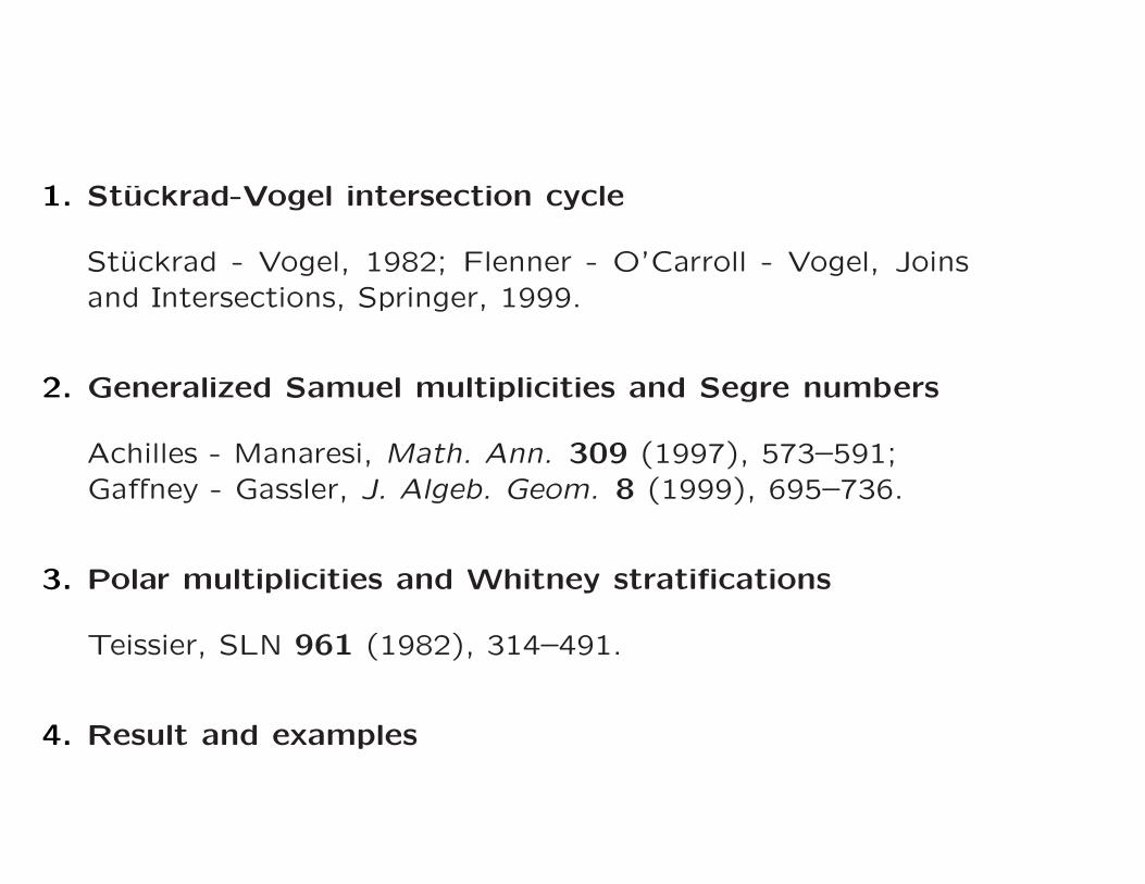
1. Stuckrad-Vogel intersection cycle

Stuckrad - Vogel, 1982; Flenner - O’Carroll - Vogel, Joins

and Intersections, Springer, 1999.

2. Generalized Samuel multiplicities and Segre numbers

Achilles - Manaresi, Math. Ann. 309 (1997), 573–591;

Gaffney - Gassler, J. Algeb. Geom. 8 (1999), 695–736.

3. Polar multiplicities and Whitney stratifications

Teissier, SLN 961 (1982), 314–491.

4. Result and examples

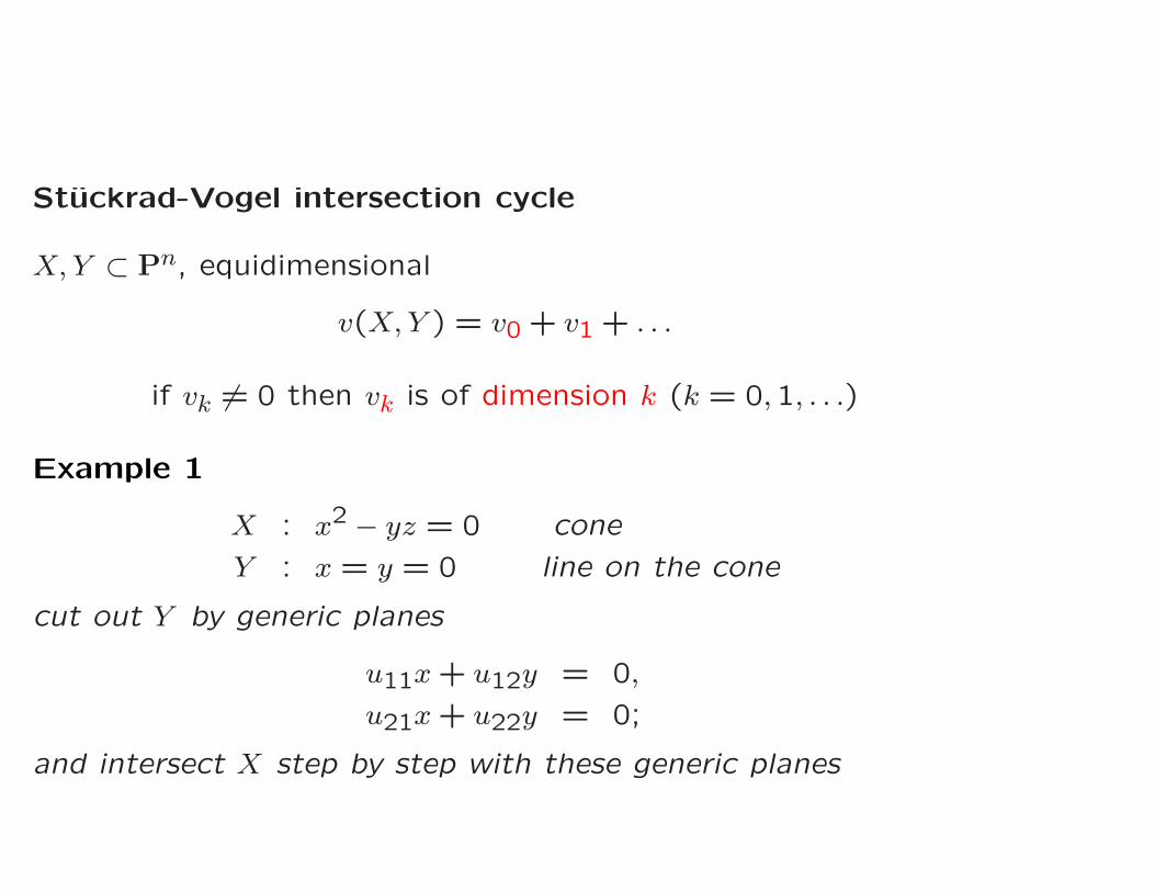
Stuckrad-Vogel intersection cycle

X, Y ⊂ Pn, equidimensional

v(X, Y ) = v0 + v1 + . . .

if vk 6= 0 then vk is of dimension k (k = 0,1, . . .)

Example 1

X : x2 − yz = 0 cone

Y : x = y = 0 line on the cone

cut out Y by generic planes

u11x + u12y = 0,

u21x + u22y = 0;

and intersect X step by step with these generic planes

components lying in X ∩Y are collected in the cycle v(X, Y ) and

the rest is intersected with the next generic plane:

First step

(x2 − yz, u11x + u12y) = (x, y) ∩ (u12x + u11z, u11x + u12y)

Second step

(u12x + u11z, u11x + u12y, u21x + u22y) = (x, y, z).

⇒ v(X, Y ) = Y + O.

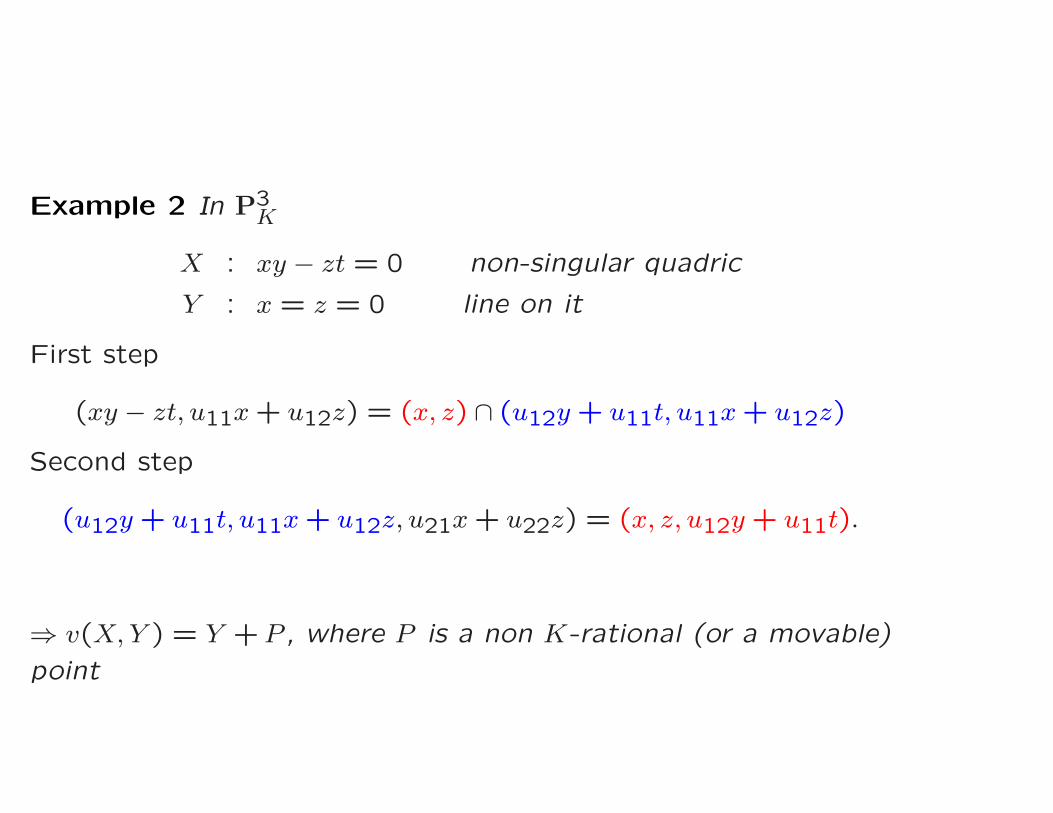
Example 2 In P3K

X : xy − zt = 0 non-singular quadric

Y : x = z = 0 line on it

First step

(xy − zt, u11x + u12z) = (x, z) ∩ (u12y + u11t, u11x + u12z)

Second step

(u12y + u11t, u11x + u12z, u21x + u22z) = (x, z, u12y + u11t).

⇒ v(X, Y ) = Y + P , where P is a non K-rational (or a movable)

point

Theorem 1 (Flenner-Manaresi, 1997) X, Y ⊂ PnK varieties,

e := dimX + dimY − n. Let k ∈ Z such that

e − 1 ≤ k ≤ dimX ∩ Y − 1, L := K(u),

p:XL ∩ YL → Pn+e−k−1L

the generic linear projection and R(p) := ramification locus of

p. Then dimR(p) ≤ k, and the associated k-cycle [R(p)]k is just

vk(X, Y ) on x ∈ X ∩ Y | X, Y, X ∩ Y smooth at x.

Definition 1

X, Y ⊆ Z closed subschemes of an algebraic K-scheme X, f :Z →N a morphism to an algebraic manifold with dimN ≥ dimX +

dimY − dimX ∩ Y . Then R(f) is defined to be the degeneracy

locus of

f∗(Ω1N) ⊗OX∩Y → Ω1

X∪Y ⊗OX∩Y .

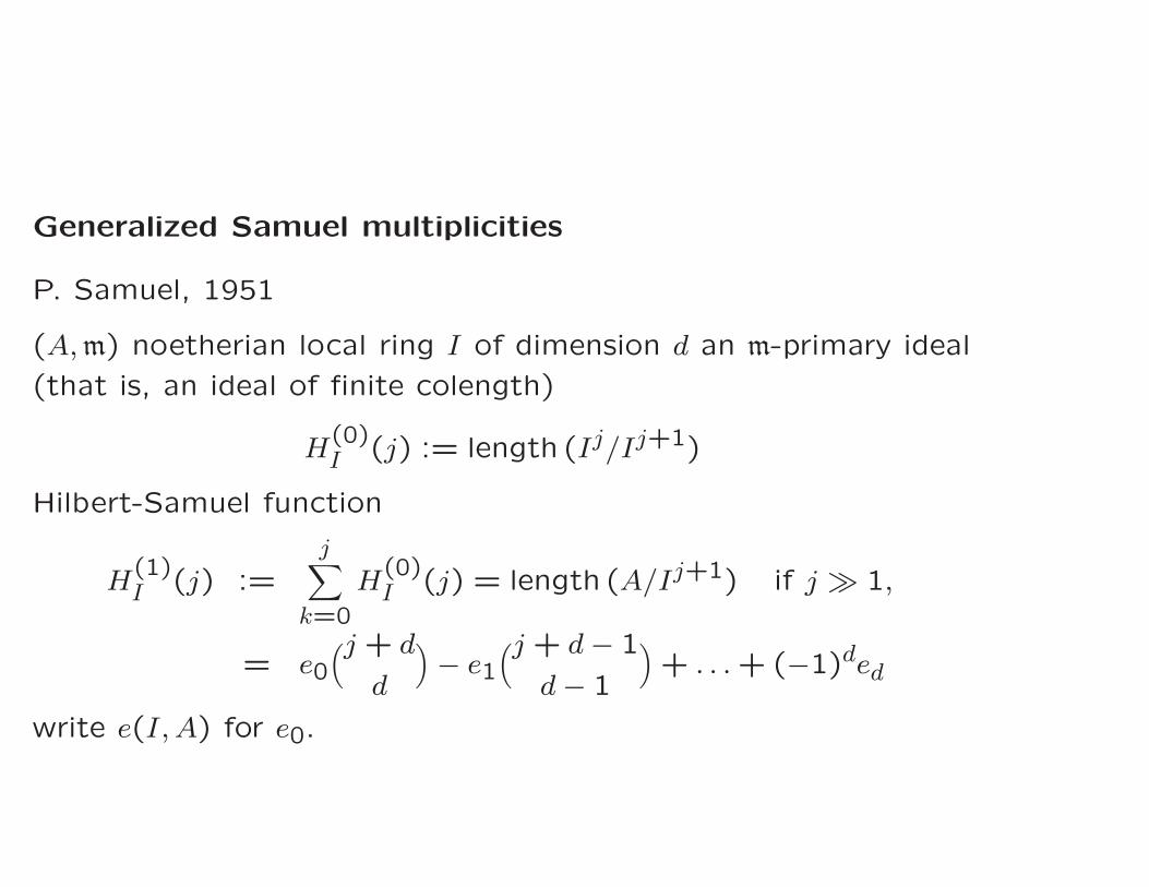
Generalized Samuel multiplicities

P. Samuel, 1951

(A, m) noetherian local ring I of dimension d an m-primary ideal

(that is, an ideal of finite colength)

H(0)I (j) := length (Ij/Ij+1)

Hilbert-Samuel function

H(1)I (j) :=

j∑

k=0

H(0)I (j) = length (A/Ij+1) if j ≫ 1,

= e0(j + d

d

)

− e1(j + d − 1

d − 1

)

+ . . . + (−1)ded

write e(I, A) for e0.

Achilles-Manaresi, 1997

I not necessarily m-primary

pass from the associated graded ring

GI(A) := ⊕j≥0Ij/Ij+1

to the bigraded ring

R = ⊕i,j≥0 Rij = Gim(G

jI(A))

= ⊕i,j≥0 (miIj + Ij+1)/(mi+1Ij + Ij+1)

R00 = A/m, have Hilbert function H(0,0)(i, j) = dimRij, twofold

sum transform H(1,1)(i, j) :=∑j

q=0

∑ip=0 H(0,0)(p, q), for both

i, j ≫ 1 becomes a polynomial which can be written in the form

∑

k+l≤d

a(1,1)k,l

(i + k

k

)(j + l

l

)

,

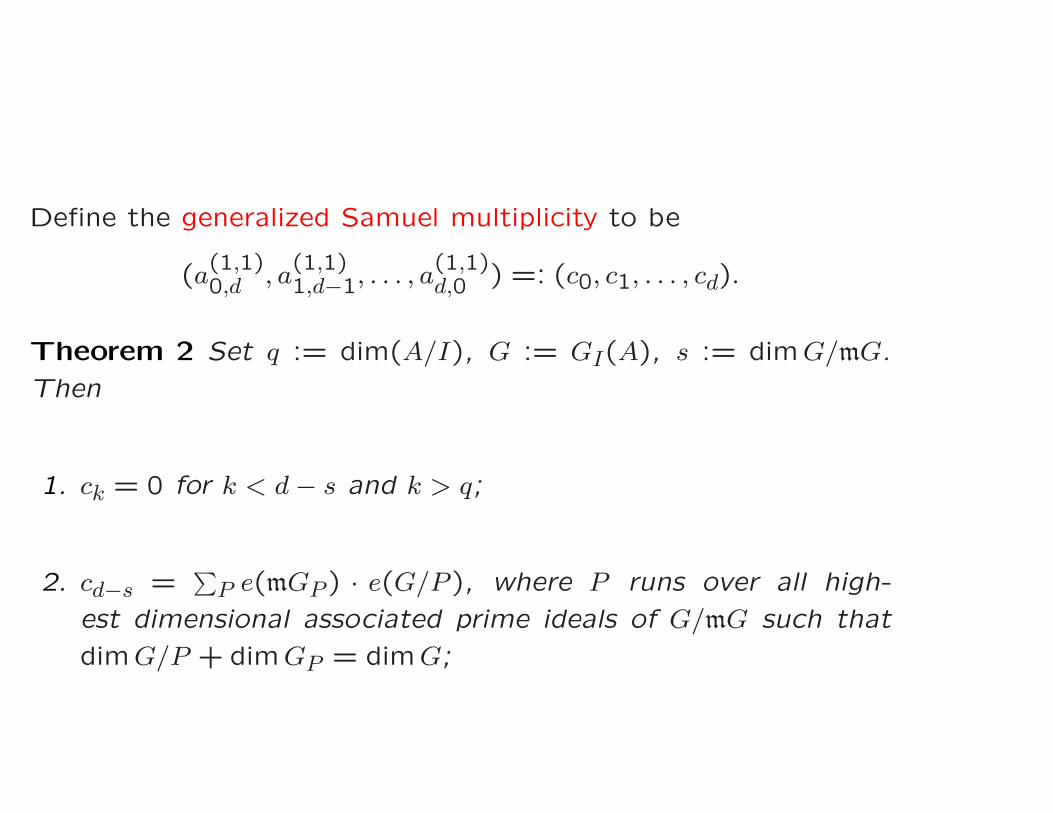
Define the generalized Samuel multiplicity to be

(a(1,1)0,d , a

(1,1)1,d−1, . . . , a

(1,1)d,0 ) =: (c0, c1, . . . , cd).

Theorem 2 Set q := dim(A/I), G := GI(A), s := dimG/mG.

Then

1. ck = 0 for k < d − s and k > q;

2. cd−s =∑

P e(mGP ) · e(G/P ), where P runs over all high-

est dimensional associated prime ideals of G/mG such that

dimG/P + dimGP = dimG;

3. cq =∑

p e(Ap) · e(A/p), where p runs over all highest dimen-

sional associated prime ideals of A/p such that dimA/p +

dimAp = dimA;

4. If A is the ring of the ruled join J := J(X, Y ) ⊂ P2n+1 (lo-

calized at the irrelevant homogeneous maximal ideal), I the

ideal of the ‘diagonal’ ∆ ⊂ P2n+1 and π: J → XY the canon-

ical projection onto the embedded join XY ⊂ Pn, then

c0 = deg∑

Γ⊆J

deg(Γ/XY ) deg(π(Γ)),

ck = deg vk−1, k = 1, . . . , d − 1 = dim J,

cd = 0.

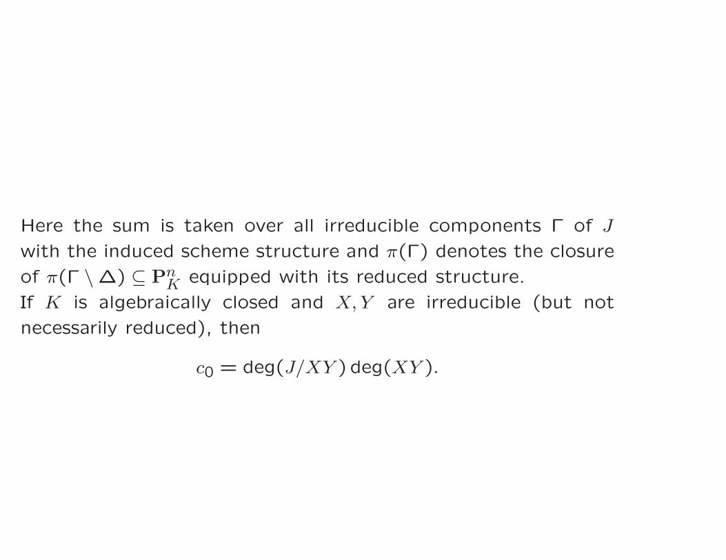
Here the sum is taken over all irreducible components Γ of J

with the induced scheme structure and π(Γ) denotes the closure

of π(Γ \ ∆) ⊆ PnK equipped with its reduced structure.

If K is algebraically closed and X, Y are irreducible (but not

necessarily reduced), then

c0 = deg(J/XY ) deg(XY ).

Segre numbers of Gaffney and Gassler, 1999

A = OX,0, (X,0) ⊂ (Cn,0) a reduced closed analytic space of

pure dimension d and I an ideal which defines a nowhere dense

subspace of (X,0). They considered the blowup of X along I

X × Pµ(I)−1 ⊃ BlI(X)

b→ X

with exceptional divisor E and defined the kth Segre number as

ek(I, Y ) := mult0(b∗(H1 · · ·Hk−1 · E · BlIX)),

where Hi is a generic hyperplane on BlIX induced by one in

Pµ(I)−1. Note that

ek(I, Y ) = cd−k(A, I), k = 1, . . . , d,

that is, Segre numbers are a special case of the generalized

Samuel multiplicity.

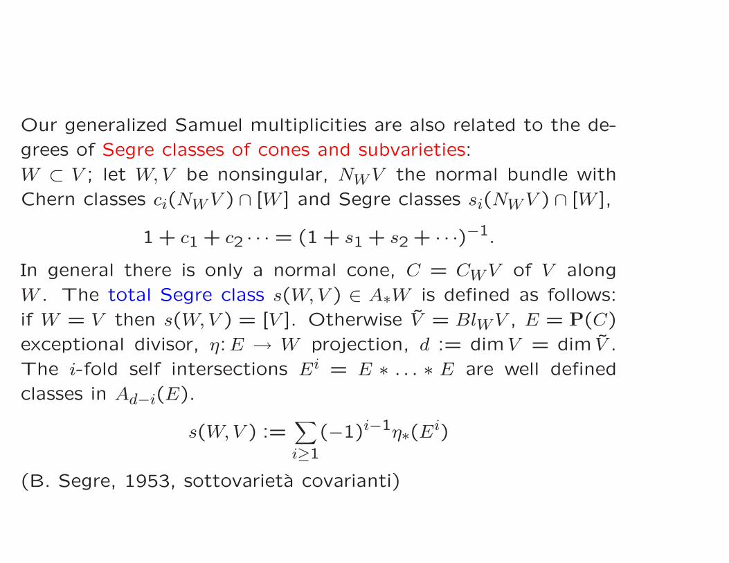
Our generalized Samuel multiplicities are also related to the de-

grees of Segre classes of cones and subvarieties:

W ⊂ V ; let W, V be nonsingular, NWV the normal bundle with

Chern classes ci(NWV ) ∩ [W ] and Segre classes si(NWV ) ∩ [W ],

1 + c1 + c2 · · · = (1 + s1 + s2 + · · ·)−1.

In general there is only a normal cone, C = CWV of V along

W . The total Segre class s(W, V ) ∈ A∗W is defined as follows:

if W = V then s(W, V ) = [V ]. Otherwise V = BlWV , E = P(C)

exceptional divisor, η:E → W projection, d := dimV = dim V .

The i-fold self intersections Ei = E ∗ . . . ∗ E are well defined

classes in Ad−i(E).

s(W, V ) :=∑

i≥1

(−1)i−1η∗(Ei)

(B. Segre, 1953, sottovarieta covarianti)

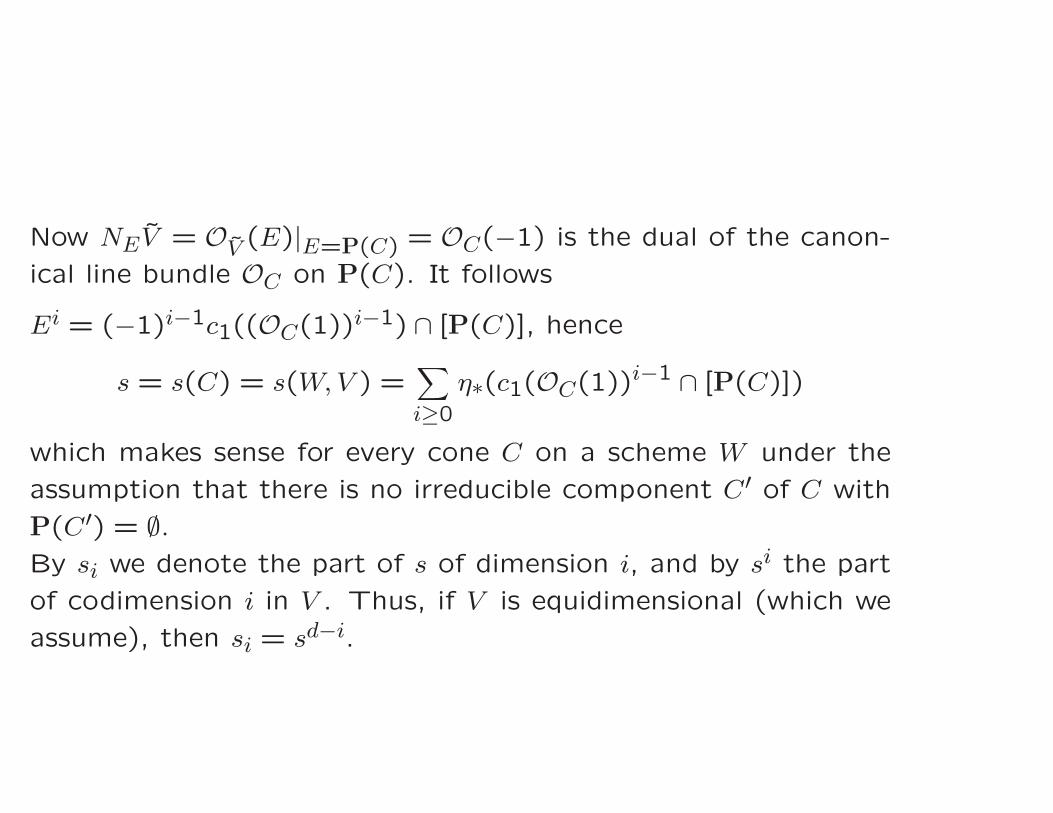
Now NEV = OV (E)|E=P(C) = OC(−1) is the dual of the canon-

ical line bundle OC on P(C). It follows

Ei = (−1)i−1c1((OC(1))i−1) ∩ [P(C)], hence

s = s(C) = s(W, V ) =∑

i≥0

η∗(c1(OC(1))i−1 ∩ [P(C)])

which makes sense for every cone C on a scheme W under the

assumption that there is no irreducible component C′ of C with

P(C′) = ∅.

By si we denote the part of s of dimension i, and by si the part

of codimension i in V . Thus, if V is equidimensional (which we

assume), then si = sd−i.

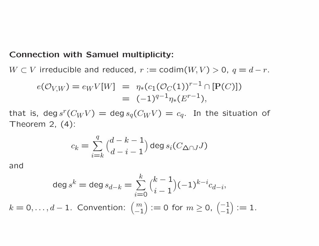
Connection with Samuel multiplicity:

W ⊂ V irreducible and reduced, r := codim(W, V ) > 0, q = d− r.

e(OV,W ) = eWV [W ] = η∗(c1(OC(1))r−1 ∩ [P(C)])

= (−1)q−1η∗(Er−1),

that is, deg sr(CWV ) = deg sq(CWV ) = cq. In the situation of

Theorem 2, (4):

ck =q

∑

i=k

(d − k − 1

d − i − 1

)

deg si(C∆∩JJ)

and

deg sk = deg sd−k =k

∑

i=0

(k − 1

i − 1

)

(−1)k−icd−i,

k = 0, . . . , d − 1. Convention:(

m−1

)

:= 0 for m ≥ 0,(

−1−1

)

:= 1.

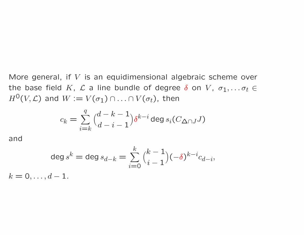
More general, if V is an equidimensional algebraic scheme over

the base field K, L a line bundle of degree δ on V , σ1, . . . σt ∈

H0(V,L) and W := V (σ1) ∩ . . . ∩ V (σt), then

ck =q

∑

i=k

(d − k − 1

d − i − 1

)

δk−i deg si(C∆∩JJ)

and

deg sk = deg sd−k =k

∑

i=0

(k − 1

i − 1

)

(−δ)k−icd−i,

k = 0, . . . , d − 1.

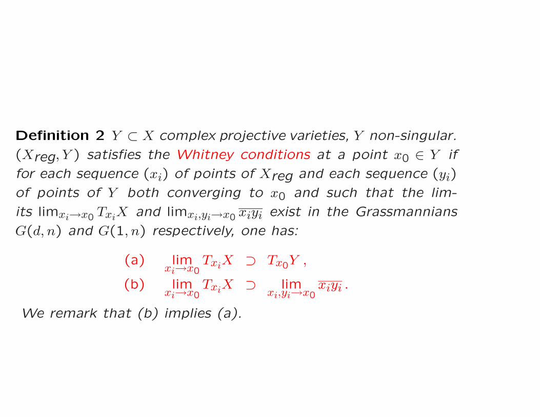
Definition 2 Y ⊂ X complex projective varieties, Y non-singular.

(Xreg, Y ) satisfies the Whitney conditions at a point x0 ∈ Y if

for each sequence (xi) of points of Xreg and each sequence (yi)

of points of Y both converging to x0 and such that the lim-

its limxi→x0 TxiX and limxi,yi→x0 xiyi exist in the Grassmannians

G(d, n) and G(1, n) respectively, one has:

(a) limxi→x0

TxiX ⊃ Tx0Y ,

(b) limxi→x0

TxiX ⊃ limxi,yi→x0

xiyi .

We remark that (b) implies (a).

Definition 3 A Whitney stratification of X (d = dimX) is given

by a filtration of X by algebraic sets Fi

X = F0 ⊇ F1 ⊇ . . . ⊇ Fd+1 = ∅

such that

(i) Fi \ Fi+1 is either empty or is a non-singular quasi-projective

variety of pure codimension i. (The connected components

of Fi \ Fi+1 are called the strata of the stratification.)

(ii) Whenever Sj and Sk are connected components of Fi \ Fi+1

and Fl \Fl+1 respectively with Sj ⊂ Sk, then the pair (Sk, Sj)

satisfies the Whitney conditions (a) and (b).

Polar varieties

L(k) = (n − d + k − 2)-dimensional linear subspace of Pn, 1 ≤

k ≤ d = dimX. The kth polar variety (or polar locus) of X

associated with L(k) is

P (Lk, X) := closure of x ∈ Xreg | dim(TxX ∩ L(k)) ≥ k − 1 .

For k = 0 we set P (L(0), X) := X.

If L(k) is generic, we write Pk(X) = P (L(k), X) and if

L(0) ⊂ L(1) ⊂ . . . ⊂ L(d)

is a generic flag, then we have

X = P0(X) ⊃ P1(X) ⊃ . . . ⊃ Pd(X) .

Let x ∈ X. Teissier showed that the sequence of multiplicities

m0 = ex(P0(X)), . . . , md−1 = ex(Pd−1(X))

does not depend upon the choice of the general flag.

Theorem 3 (Teissier, 1982) The pair (Xreg, Y ) satisfies the

Whitney conditions in x0 if and only if the sequence of polar

multiplicities

m0 = ey(X), m1 = ey(P1(X)), . . . , md−1 = ey(Pd−1(X))

is locally constant in Y around x0.

We propose the following function g to measure the singularity

of X in a point x of X:

A := OX×X,(x,x), I := diagonal ideal in A,

g(x) :=d

∑

i=0

ci(I, A) = e(GI(A)).

Note that dimA = 2d, cd+1 = · · · = c2d = 0 and that

(c0(I, A), c1(I, A), . . . , cd(I, A))

is a refinement of the multiplicity

cd(I, A) = exX = e(OX,x)

of X at x.

Theorem 4 (Achilles-Manaresi, 2003) Let X ⊂ Pn be a (re-

duced) surface and x ∈ X be a closed point. Then

Xj := x ∈ X | g(x) ≥ j, j = 0,1, . . .

are closed subschemes of X or empty, and the connected com-

ponents of

Sg(j) := g−1(j) = Xj \ Xj+1

are the strata of a Whitney stratification of X (the coarsest one

if n = 3).

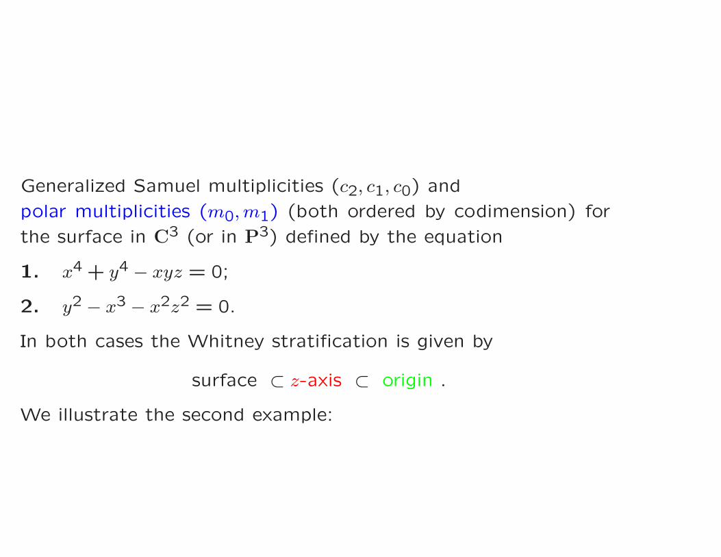
Generalized Samuel multiplicities (c2, c1, c0) and

polar multiplicities (m0, m1) (both ordered by codimension) for

the surface in C3 (or in P3) defined by the equation

1. x4 + y4 − xyz = 0;

2. y2 − x3 − x2z2 = 0.

In both cases the Whitney stratification is given by

surface ⊂ z-axis ⊂ origin .

We illustrate the second example:

z6

y¼ x

-

x

(2,2,0) (2,0)

x

(1,0,0) (1,0)

x

(2,3,0) (2,1)