Computation of 3D weld pool surface from the slope field and point

INSTITUTE OF PHYSICS PUBLISHING MEASUREMENT SCIENCE AND TECHNOLOGY

Meas. Sci. Technol. 15 (2004) 389–403 PII: S0957-0233(04)66893-7

Computation of 3D weld pool surfacefrom the slope field and point tracking oflaser beamsG Saeed, M Lou and Y M Zhang

Center for Manufacturing and Department of Electrical and Computer Engineering,College of Engineering, University of Kentucky, Lexington, KY 40506, USA

E-mail: [email protected]

Received 31 July 2003, in final form 20 November 2003, accepted forpublication 3 December 2003Published 19 December 2003Online at stacks.iop.org/MST/15/389 (DOI: 10.1088/0957-0233/15/2/012)

AbstractA novel computation method of the 3D weld pool surface from specularreflection of laser beams is presented in this paper. The mathematical modelfor the three-dimensional surface measurement technique has beendeveloped. The structured pattern of a laser is projected on the weld pool ina molten state and the reflection observed using a CCD camera. Thesereflected patterns can be tracked using image processing techniquesincluding optical flow and moving point tracking. A simulation model hasbeen developed implementing these techniques. The movement of thereflected laser during the welding process is indicative of the change in stateof the weld pool. The surface slope field is calculated from the law ofreflection and is used to compute the 3D surface of the weld pool. Themeasurement technique is tested on objects with a priori knowledge ofgeometry having a specular surface to test the effectiveness of themeasurement technique.

Keywords: structured light, welding, surface

(Some figures in this article are in colour only in the electronic version)

1. Introduction

Welding has become an indispensable tool for many industriesbecause of the basic role of joining of materials in themanufacturing industry. Some welding techniques, such asgas tungsten arc welding (GTAW), produce high quality welds.For critical and accurate joining where the weld quality mustbe ensured such as for the root pass and for the welding ofadvanced materials, GTAW is often used to produce a high-quality weld because of its capability in precision control ofthe fusion process [1].

In an arc welding process, the electric arc heats the workpiece and the molten pool. The temperature gradient onthe pool surface creates a difference in the surface tensionthat drives the liquid metal flow. The electromagnetic forceassociated with the welding current flow also drives the liquidmetal flow. The fluid flow driven convection, which isthe major heat transfer form in the weld pool, controls the

geometry of the fusion zone. Further, the geometry of thefusion zone determines how the weld pool surface is deformedunder arc pressure and gravity. The deformation of the weldpool is a determining factor for the distribution of the arc andthe distribution of the current flow (thus the electromagneticforce). Finally, the surface tension depends on the deformationof the weld pool surface and the distribution of the arc (heatinput flux and the temperature field). Hence, a chain reactionand strong coupling of heat transfer, fluid flow, and geometricaldeformation exists in the weld pool. The physical processesoccurring in the weld pool are very complicated.

Due to the extreme complexity, analytic methods ingeneral cannot adequately describe the physical phenomenaassociated with arc welding processes. Numerical analysishas been a powerful tool in modelling these phenomenaand revealing their fundamentals. However, in order toconfirm the effectiveness of the numerical models, thecalculated results must be compared with experimental data.

0957-0233/04/020389+15$30.00 © 2004 IOP Publishing Ltd Printed in the UK 389

http://stacks.iop.org/MST/15/389

G Saeed et al

Ideally, experimental data for temperature field [2, 3], fluidflow [4, 5], fusion zone geometry [6, 7], and pool surfacedeformation [4, 8–11] are all required.

Although the temperature field and the fusion zonegeometry can be measured using existing methods, theobservation and measurement of the deformation of thepool surface and the fluid flow in the weld pool remaindifficult. The strong illumination from the arc disqualifiesmost visual technologies for possible applications in arcwelding. The specular surface of the weld pool adds anotherdifficulty. Hence, despite the importance of observation andmeasurement of fluid flow and the pool surface, only limitedsolutions have been obtained to date. This paper will focus onthe measurement of the surface of the weld pool, which willsignificantly benefit the development of the numerical models.

To measure the three-dimensional surface of the weldpool, a sensing system was developed at the Universityof Kentucky using a specific high shutter speed camerasystem and a specific optic grid which consists of a gridand frosted glass [12, 13]. A recent study has been done tomathematically model this sensing system in order to optimizethe design [14]. While this measurement system can visualizethe three-dimensional pool surface by the deformed laserstripes projected through the specific optic grid, it requiresa specific camera system whose shutter is synchronized witha pulsed laser so that the intensity of the laser stripes is muchstronger than that of the arc during imaging. The acquiredquality image of the weld pool surface makes this systemsuitable for laboratory studies, but the high capital investmentof the specific camera system affects its affordability in real-time control applications. To develop a cost-effective systemfor real-time control applications, this paper proposes a novelsensing technique which only uses a high-speed digital cameraand laser and requires no synchronization between the cameraand laser. Band pass filters centred at the laser beam’swavelength are mounted on the camera to prevent the arc lightand other light sources from entering the camera.

This paper is organized as follows: section 2 providesa description of the sensing technique. In section 3, themathematical model of the weld pool will be ascertained. Insection 4, the optical flow tracking method will be introduced.Section 5 will use the optical flow concepts from imageprocessing to analyse the optical points moving in the plane.The reflected points will be used to calculate the slope field ofthe weld pool surface and the 3D surface reconstructed fromthe slope field in section 6. Section 7 will conclude all of theabove work and present ideas for future work.

2. Description of proposed sensing technique

In the proposed sensing technique, a laser is used to illuminatethe weld pool surface. The corresponding reflected raysare completely determined by the slope of the weld poolinterface and the point where they hit the weld pool (alsocalled the intersection points). Figure 1 illustrates the sensingmechanism used. By tracking the reflected rays and computingthe slope field of the weld pool surface, the three-dimensionalweld pool shape can be determined.

In the laboratory setting, an He–Ne laser connected toprojector adapters is used to create a set of parallel incident

Figure 1. Proposed observation approach.

laser beams in the form of a laser dot matrix. The laser dotmatrix is set to cover the weld pool surface area entirely. Whenthese rays hit the solid base metal, their specular reflection isnegligible. Those which hit the liquid metal surface of theweld pool are almost completely reflected. Since the angleand position of the incident laser rays have already been set,and if the equation of the reflected ray is known, the reflectedpoint including its slope and position in the three-dimensionalworld can be determined based on the direction of the incidentrays and the reflection law.

The equation of a reflected ray in the three-dimensionalworld can be determined by knowing any two points on it.A method using dual planes to intercept two points in thereflection path was considered initially. The image of areflected ray on the two planes gives two points on it. As a resultthe reflected ray can be directly determined from the imageswithout substantial computation. But due to the limitation ofthis method, which was the inability of the camera to get clearimages of both the planes at the same time, this method wasnot used. In this paper, an algorithm will be proposed based onobserving only one plane which intersects the reflected rays.The reflected rays will be constructed using an approximationand the location of this one point.

The movement of the reflected laser on the intersectionplane can be tracked to monitor the state of the three-dimensional weld pool surface. During welding, the points onthe plane will move with the change of the weld pool surface.Some points may disappear or reappear and some of themwill change their relative positions. Tracking these points is atypical feature point tracking problem in pattern recognition.Given a sequence of frames corresponding to a dynamic scene,multi-frame correspondence of a set of selected image points,called feature points of interest, is used to determine the motiontrajectories of those points. This paper tries to synthesizesome of the existing algorithms for finding and tracking featurepoints.

3. Mathematical model and optical theory

3.1. Mathematical model

The welding electrode is considered to be above the work piecein the z direction and it moves in the x direction at a constantspeed u. A moving coordinate system is so chosen that itsorigin is at the centre of the welding electrode. The equationthat governs the balance at the liquid–vapour and solid–liquid

390

Computation of 3D weld pool surface from the slope field and point tracking of laser beams

Figure 2. Three-dimensional solid–liquid weld pool (front view). The weld pool surface is shallow because its depth is 0.05 mm while itswidth is 4 mm.

interfaces under the quasi-steady state condition is used toobtain the shapes of these interfaces [4, 8–11]. The solid–liquid interface Ss(x, y) is given below as

Ss(x, y) = Ks

2Lm

(AP

πρv

) 23(

Lm + Cp(Tm − T0)

3R0

) 13

× exp

(−2(x + 2R0 Pes)

2

d2s

)exp

(−2y2

L2s

)(1)

where ds = Ls − 2R0 if x � −2R0 Pes, else ds = Ls + 2R0,Ks and Ls are given by

Ks = [Lm + Cp(Tm − T0)]2

Lm[Lb + Lm + Cp(Tm − T0)];

Ls =(

3AP R0

πρv[Lb + Lm + Cp(Tm − T0)]

) 13

,

and Pes is defined as the Peclet parameter and is given byPes = vR0

as[14].

The other parameters with their values are summarized intable 1.

The width of the weld is typically considered to be thewidth of the solid–liquid interface profile at the surface ofthe work piece. Figure 2 shows a Matlab simulation ofequation (1) to obtain the three-dimensional solid–liquid weldpool interface.

It should be pointed out that the above analytical modelsare derived from laser welding. Although laser weld poolsare in general different from those of a gas tungsten arc,shallow laser weld pools generated by a low power, defocused(large diameter) beam should be similar to those of a gastungsten arc. Further, the focus of the present research isto measure three-dimensional surfaces of weld pools andthe measurement system is modelled to study the effect ofthe system parameters on measurement results. The surfaceof the weld pool is given only as input parameters. Moreimportantly and practically, limited work has been done toestablish analytical models for gas tungsten arc weld pools.Hence, the analytical models derived from laser welding are

Table 1. Values of parameters used in the weld pool equation.

Values of thermo-Name and notation physical properties

Power, P (W ) 2000Density, ρ (kg m−3) 7500 (7000)

liquid (solid) stateMelting temperature, Tm (K) 1810Boiling temperature, Tb (K) 3342Work piece initial temperature, T0 (K) 50Specific heat capacitance, Cp (J kg−1 K−1) 678.5 (636.7)Latent heat of fusion, Lm (J kg−1) 2.72 × 105

Latent heat of boiling, Lb (J kg−1) 6.3 × 106

Diffusivity for the liquid state, αl (m2 s−1) 5.223 × 10−6

Diffusivity for the solid state, αs (m2 s−1) 6.435 × 10−6

Radius or arc/laser, R0 (m) 0.0003Speed of welding, v (m s−1) 0.02

used to approximate gas tungsten weld pool surfaces using anenergy beam wider than typical laser applications in this paper.

3.2. Optical geometry

3.2.1. Incident line. The incident laser rays are described bydirection vectors and the coordinates of the laser source point.

xi, j (t) = xi, j (0) + px × t,

yi, j (t) = yi, j (0) + py × t

zi, j (t) = zi, j (0) + pz × t

(2)

where [xi, j (0),yi, j (0), zi, j (0)] represents the coordinates of alaser source in the real world and [px , py, pz] is the directionvector of the laser beam. The parameter t is an independentvariable.

3.2.2. Normal line [15, 16]. Suppose S is a surface withequation F(x, y, z) = n. Let P = (x0, y0, z0) be a pointon S. Let C be any curve that lies on surface S and passesthrough point P . Curve C is described by a continuous vector

391

G Saeed et al

function r(t) = (x(t), y(t), z(t)). Let t0 be the parametervalue corresponding to P ; that is r(t0) = (x0, y0, z0). Since Clies on S, any point (x(t), y(t), z(t)) must satisfy the equationfor S, that is,

F(x(t), y(t), z(t)) = n. (3)

If x , y and z are differentiable functions of t and F is alsodifferentiable, then the chain rule can be used to differentiateboth sides as follows:

∂ F

∂x

dx

dt+

∂ F

∂y

dy

dt+

∂ F

∂z

dz

dt= 0. (4)

However, since ∇ F = (Fx , Fy, Fz) and r ′(t) = (x ′(t),y ′(t), z′(t)), the above equation can be written in terms of adot product as ∇ F · r ′(t) = 0. In particular, when t = t0,r(t0) = (x0, y0, z0), then

∇ F(x0, y0, z0) · r ′(t0) = 0. (5)

This implies that the gradient vector ∇ F(x0 , y0, z0) at P istangent to vector r ′(t0) at any curve C on S that passes throughP . Since ∇ F(x0, y0, z0) �= 0, it is natural to define the tangentplane to F(x(t), y(t), z(t)) = k at P as the plane that passesthrough P and has normal vector ∇ F(x0, y0, z0). The normalline to S at P is the line passing through P and perpendicularto tangent plane. The direction of the normal line is thereforegiven by the gradient vector ∇ F(x0, y0, z0) and its symmetricequations are thus

x − x0

Fx(x0, y0, z0)= y − y0

Fy(x0, y0, z0)= z − z0

Fz(x0, y0, z0). (6)

In the special case in which the equation of a surface Sis of the form z = f (x, y) (that is, S is a function f of twovariables), the equation can be rewritten as

F(x, y, z) = f (x, y) − z = 0 (7)

and we consider S as a weld pool surface with equationz = f (x, y). Then

Fx(x0, y0, z0) = fx (x0, y0)

Fy(x0, y0, z0) = f y(x0, y0)

Fz(x0, y0, z0) = −1.

(8)

3.2.3. Reflected line. The reflected lines were calculatedbased on the law of reflection, which states that the incidentangle of a light beam is equal to the angle of reflection. Figure 3illustrates this concept where θi is equal to θr.

From figure 3, suppose ki is the angle of the incident raymeasured from the horizon and θ is the slope angle of the weldpool interface. Then,

θr = θi = π

2− ki + θ. (9)

The angle of the reflected line from the horizon is

kr = π − ki + 2θr. (10)

The function of the reflected line can be written as

xr = tan(krx ) × t + xinter

yr = tan(kry) × t + yinter

zr = t + zinter

(11)

normal line

reflected beamincident beam

tangent

θθ

θθ

ri

Figure 3. Reflected rays from a weld pool interface.

where (xinter, yinter, zinter) is the intersection point of theincident ray and the reflector; krx and kry are kr (the angle of theslope of the reflected line) in x and y directions respectively.

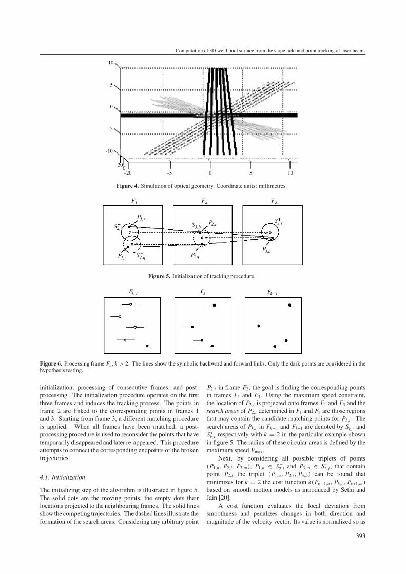
Figure 4 shows a simulation of the proposed method byMatlab. In the figure, dotted lines represent a set of parallelincident laser beams which illuminate the 3D weld pool surfaceof figure 2. The dark bold lines represent the normal lines ofthe weld pool surface, and the remaining lines represent thereflected laser beams.

4. Feature point tracking [18]

If only one incident ray is used to illuminate the weld pool,there will be only one reflected point on the plane. However,in the proposed method, a set of laser rays is used which, afterreflection, creates a dot matrix of reflected points on the imageplane. While the size and shape of these dots may not changesignificantly, the pattern formed by them will be distorted andthus vary as the weld pool surface changes. For the rays whichhit the solid base metal or solidified weld metal, the specularreflection is negligible. Rays that hit the liquid metal surfaceof the weld pool will reflect nearly completely. As a result,the reflected points may temporarily disappear, group, enteror leave the field of view. The reflected points can be calledfeature points or points of interest. This section will discusshow to determine the motion trajectories of those points whengiven a sequence of frames.

Typically, the characteristics of the motion of featurepoints are classified and described using different motionmodels, such as the average deviation conditioned bycompetition and alternative model [17], the smooth motionmodel [20], and the proximal uniformity model [17]. Manyalgorithms or methods are provided based on the motionmodels.

Feature point based motion tracking was used, in thelong image sequences algorithm in which dynamic sceneswith multiple independently moving objects are consideredand feature points may temporarily disappear, enter and leavethe field of view. Most of the existing approaches to featurepoint tracking have limited capabilities in handling incompletetrajectories especially when the number of points and theirspeeds are large and trajectory ambiguities are frequent.The basic matching algorithm has three basic steps [18–20]:

392


10-20

-10

20

5

5

-5

-5

0

0

0

10

Figure 4. Simulation of optical geometry. Coordinate units: millimetres.

F1 F2 F3

S SS

S

PP

PPP1,r

1,r

2,q 2,q

3,b

3,b

2,i2,i

2,i

Figure 5. Initialization of tracking procedure.

Fk-1 Fk+1Fk

Figure 6. Processing frame Fk , k > 2. The lines show the symbolic backward and forward links. Only the dark points are considered in thehypothesis testing.

initialization, processing of consecutive frames, and post-processing. The initialization procedure operates on the firstthree frames and induces the tracking process. The points inframe 2 are linked to the corresponding points in frames 1and 3. Starting from frame 3, a different matching procedureis applied. When all frames have been matched, a post-processing procedure is used to reconsider the points that havetemporarily disappeared and later re-appeared. This procedureattempts to connect the corresponding endpoints of the brokentrajectories.

4.1. Initialization

The initializing step of the algorithm is illustrated in figure 5.The solid dots are the moving points, the empty dots theirlocations projected to the neighbouring frames. The solid linesshow the competing trajectories. The dashed lines illustrate theformation of the search areas. Considering any arbitrary point

P2,i in frame F2, the goal is finding the corresponding pointsin frames F1 and F3. Using the maximum speed constraint,the location of P2,i is projected onto frames F1 and F3 and thesearch areas of P2,i determined in F1 and F3 are those regionsthat may contain the candidate matching points for P2,i . Thesearch areas of Pk,i in Fk−1 and Fk+1 are denoted by S−

k,i andS+

k,i respectively with k = 2 in the particular example shownin figure 5. The radius of these circular areas is defined by themaximum speed Vmax.

Next, by considering all possible triplets of points(P1,n, P2,i , P3,m), P1,n ∈ S−

2,i and P3,m ∈ S+2,i , that contain

point P2,i the triplet (P1,a, P2,i , P3,b) can be found thatminimizes for k = 2 the cost function δ(Pk−1,n, Pk,i , Pk+1,m)

based on smooth motion models as introduced by Sethi andJain [20].

A cost function evaluates the local deviation fromsmoothness and penalizes changes in both direction andmagnitude of the velocity vector. Its value is normalized so as

393

G Saeed et al

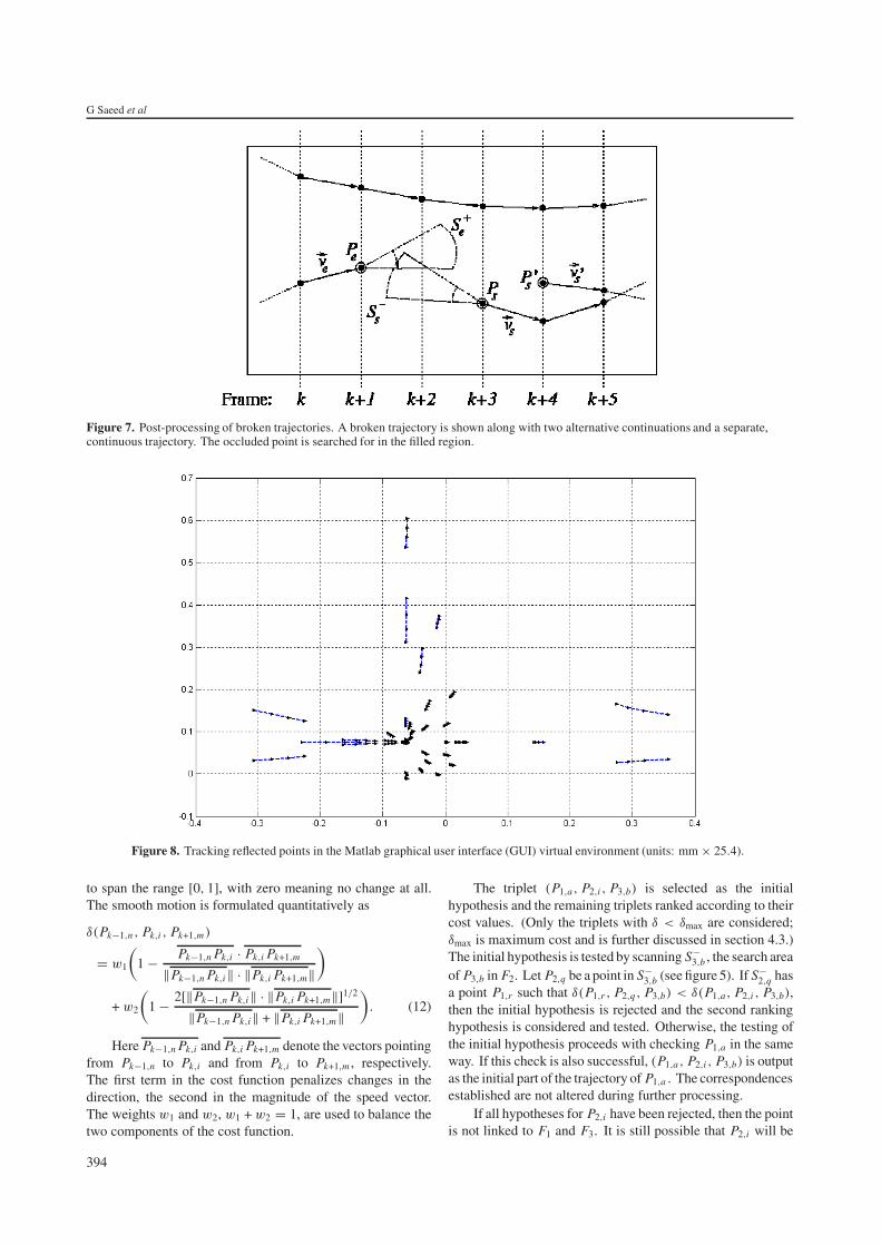
Figure 7. Post-processing of broken trajectories. A broken trajectory is shown along with two alternative continuations and a separate,continuous trajectory. The occluded point is searched for in the filled region.

Figure 8. Tracking reflected points in the Matlab graphical user interface (GUI) virtual environment (units: mm × 25.4).

to span the range [0, 1], with zero meaning no change at all.The smooth motion is formulated quantitatively as

δ(Pk−1,n , Pk,i , Pk+1,m)

= w1

(1 − Pk−1,n Pk,i · Pk,i Pk+1,m

‖Pk−1,n Pk,i‖ · ‖Pk,i Pk+1,m‖)

+ w2

(1 − 2[‖Pk−1,n Pk,i‖ · ‖Pk,i Pk+1,m‖]1/2

‖Pk−1,n Pk,i‖ + ‖Pk,i Pk+1,m‖)

. (12)

Here Pk−1,n Pk,i and Pk,i Pk+1,m denote the vectors pointingfrom Pk−1,n to Pk,i and from Pk,i to Pk+1,m , respectively.The first term in the cost function penalizes changes in thedirection, the second in the magnitude of the speed vector.The weights w1 and w2, w1 + w2 = 1, are used to balance thetwo components of the cost function.

The triplet (P1,a, P2,i , P3,b) is selected as the initialhypothesis and the remaining triplets ranked according to theircost values. (Only the triplets with δ < δmax are considered;δmax is maximum cost and is further discussed in section 4.3.)The initial hypothesis is tested by scanning S−

3,b , the search areaof P3,b in F2. Let P2,q be a point in S−

3,b (see figure 5). If S−2,q has

a point P1,r such that δ(P1,r , P2,q, P3,b) < δ(P1,a, P2,i , P3,b),then the initial hypothesis is rejected and the second rankinghypothesis is considered and tested. Otherwise, the testing ofthe initial hypothesis proceeds with checking P1,a in the sameway. If this check is also successful, (P1,a, P2,i , P3,b) is outputas the initial part of the trajectory of P1,a . The correspondencesestablished are not altered during further processing.

If all hypotheses for P2,i have been rejected, then the pointis not linked to F1 and F3. It is still possible that P2,i will be

394


Optical flow

Reflected laserfrom Surface 1

Reflected laserfrom Surface2 Normal line

Surface 1

Normal line ofSurface 1

Normal line ofSurface 2

Opticalflow



Interface depthchange

Incident laserbeam

Surface 1Surface 2

Slope direction

Normal line of Surface 2

Incident laserbeam

Surface 2

Surface 1

(a) (b)

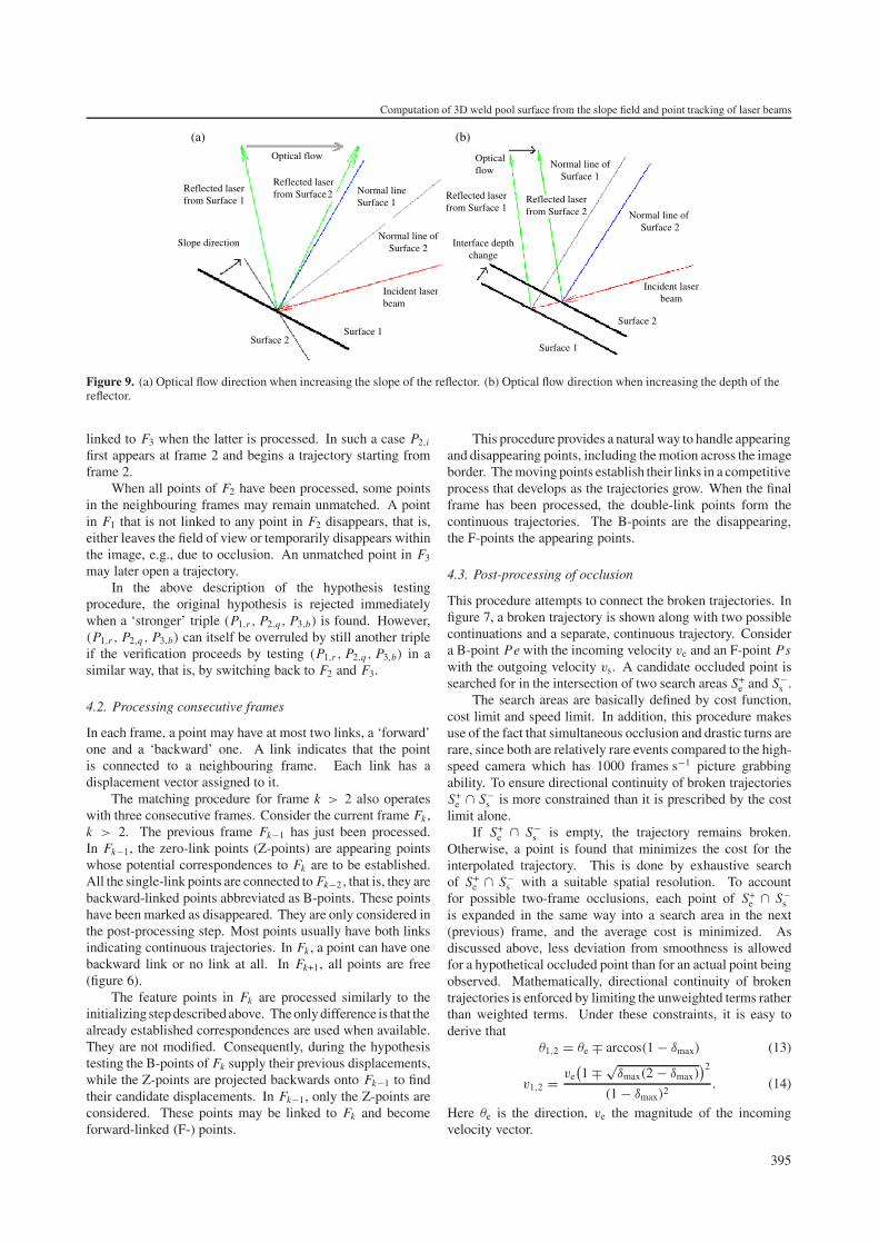
Figure 9. (a) Optical flow direction when increasing the slope of the reflector. (b) Optical flow direction when increasing the depth of thereflector.

linked to F3 when the latter is processed. In such a case P2,i

first appears at frame 2 and begins a trajectory starting fromframe 2.

When all points of F2 have been processed, some pointsin the neighbouring frames may remain unmatched. A pointin F1 that is not linked to any point in F2 disappears, that is,either leaves the field of view or temporarily disappears withinthe image, e.g., due to occlusion. An unmatched point in F3

may later open a trajectory.In the above description of the hypothesis testing

procedure, the original hypothesis is rejected immediatelywhen a ‘stronger’ triple (P1,r , P2,q, P3,b) is found. However,(P1,r , P2,q , P3,b) can itself be overruled by still another tripleif the verification proceeds by testing (P1,r , P2,q , P3,b) in asimilar way, that is, by switching back to F2 and F3.

4.2. Processing consecutive frames

In each frame, a point may have at most two links, a ‘forward’one and a ‘backward’ one. A link indicates that the pointis connected to a neighbouring frame. Each link has adisplacement vector assigned to it.

The matching procedure for frame k > 2 also operateswith three consecutive frames. Consider the current frame Fk ,k > 2. The previous frame Fk−1 has just been processed.In Fk−1, the zero-link points (Z-points) are appearing pointswhose potential correspondences to Fk are to be established.All the single-link points are connected to Fk−2 , that is, they arebackward-linked points abbreviated as B-points. These pointshave been marked as disappeared. They are only considered inthe post-processing step. Most points usually have both linksindicating continuous trajectories. In Fk , a point can have onebackward link or no link at all. In Fk+1, all points are free(figure 6).

The feature points in Fk are processed similarly to theinitializing step described above. The only difference is that thealready established correspondences are used when available.They are not modified. Consequently, during the hypothesistesting the B-points of Fk supply their previous displacements,while the Z-points are projected backwards onto Fk−1 to findtheir candidate displacements. In Fk−1, only the Z-points areconsidered. These points may be linked to Fk and becomeforward-linked (F-) points.

This procedure provides a natural way to handle appearingand disappearing points, including the motion across the imageborder. The moving points establish their links in a competitiveprocess that develops as the trajectories grow. When the finalframe has been processed, the double-link points form thecontinuous trajectories. The B-points are the disappearing,the F-points the appearing points.

4.3. Post-processing of occlusion

This procedure attempts to connect the broken trajectories. Infigure 7, a broken trajectory is shown along with two possiblecontinuations and a separate, continuous trajectory. Considera B-point Pe with the incoming velocity ve and an F-point Pswith the outgoing velocity vs. A candidate occluded point issearched for in the intersection of two search areas S+

e and S−s .

The search areas are basically defined by cost function,cost limit and speed limit. In addition, this procedure makesuse of the fact that simultaneous occlusion and drastic turns arerare, since both are relatively rare events compared to the high-speed camera which has 1000 frames s−1 picture grabbingability. To ensure directional continuity of broken trajectoriesS+

e ∩ S−s is more constrained than it is prescribed by the cost

limit alone.If S+

e ∩ S−s is empty, the trajectory remains broken.

Otherwise, a point is found that minimizes the cost for theinterpolated trajectory. This is done by exhaustive searchof S+

e ∩ S−s with a suitable spatial resolution. To account

for possible two-frame occlusions, each point of S+e ∩ S−

sis expanded in the same way into a search area in the next(previous) frame, and the average cost is minimized. Asdiscussed above, less deviation from smoothness is allowedfor a hypothetical occluded point than for an actual point beingobserved. Mathematically, directional continuity of brokentrajectories is enforced by limiting the unweighted terms ratherthan weighted terms. Under these constraints, it is easy toderive that

θ1,2 = θe ∓ arccos(1 − δmax) (13)

v1,2 = ve(1 ∓ √

δmax(2 − δmax))2

(1 − δmax)2. (14)

Here θe is the direction, ve the magnitude of the incomingvelocity vector.

395

G Saeed et al

Figure 10. Optical flow of reflected rays (units mm ×25.4).

Figure 11. Rays diverging after passing through the focal centre ofa concave mirror.

From these equations, the maximum allowed directionchange for broken trajectories is π/2, when δmax = 1. Whenδmax = 0.5, the turn limit is π/3. 0 � v1 � ve, while v2 � ve.When δmax is set close to unity, v1 ≈ 0 and v2 ve.

4.4. Tracking reflected points by Matlab simulation

In equation (1), if the welding current is changed (113–120–126–133 A), then the weld pool interface will be distorted.With increasing current, the depth of the weld pool willincrease, and at the same time, the reflected lines from theinterface will change their direction. The intersection points ofreflected lines on the image plane will move with the distortionof the weld pool surface. Using the above tracking method,the movement of every intersection point can be tracked inthe Matlab simulation, as shown in figure 8. The dots are theposition of feature points at each state, and the connecting lineshows the correspondence established between them by thetracking algorithm.

Figure 12. Simplification of coordinates for a reflected point.

5. Optical flow [21–24]

Optical flow is the apparent motion of brightness patternsacross the image plane of a computer vision system or acrossthe retina of the eye in a biological vision system. Opticalflow arises from movement of objects in the scene or frommovement of the camera (or eye) through the scene.

Calculation of the optical flow is used as a cue to aidthe processing of video segmentation. In this case, since theilluminating laser source is fixed in position and angle duringthe experiment, the movement of the feature points created bythe reflected beams can be seen as the optical flow, or in otherwords, the motion field.

5.1. Estimation of optical flow

Assume the weld pool surface is stationary and can be modelledby a mathematical equation, which can be written as a functionF(x, y, z,), and assume that X is the coordinate matrix of theprojected pattern (the 3D space position of a set of parallel laserbeams), and X ′ the coordinate matrix after reflection, then the

396


(a)

(b)

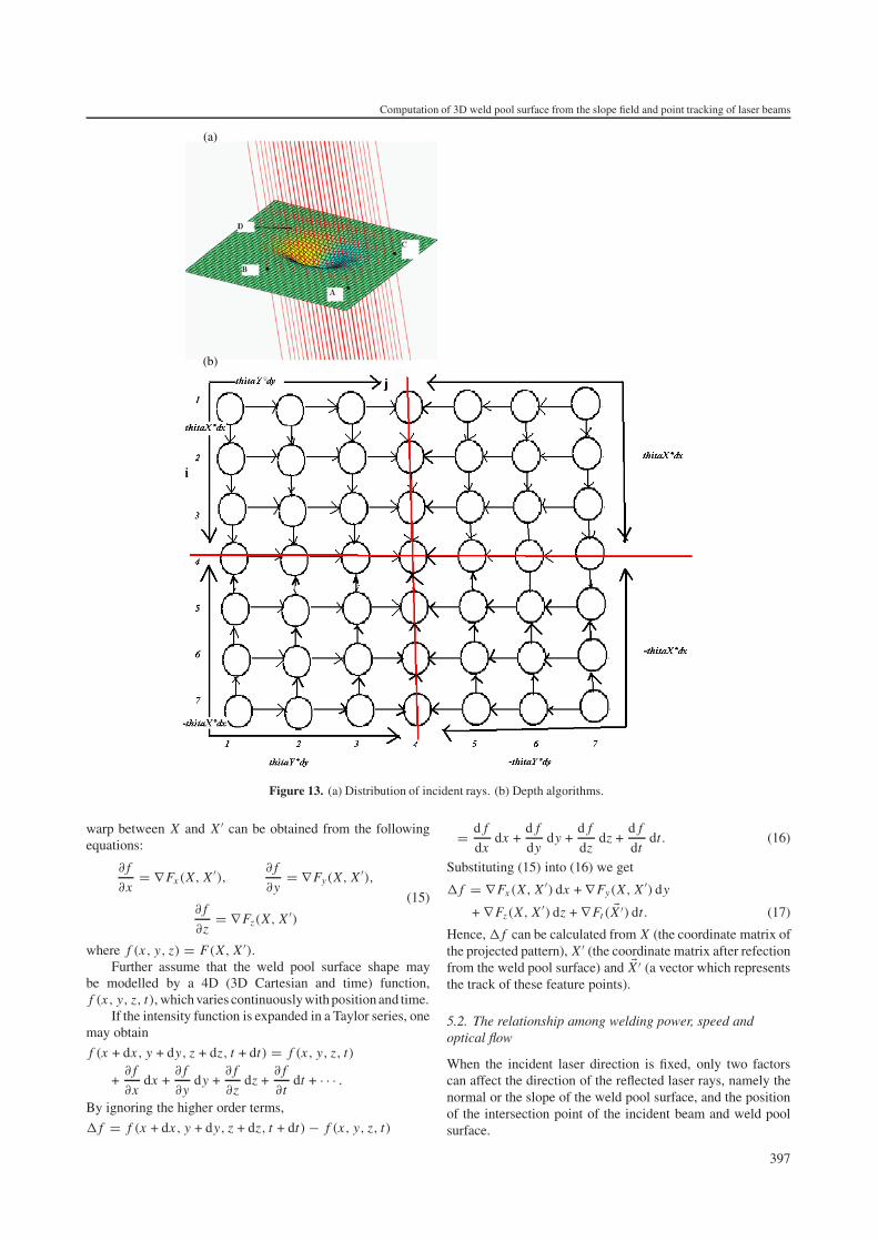
Figure 13. (a) Distribution of incident rays. (b) Depth algorithms.

warp between X and X ′ can be obtained from the followingequations:

∂ f

∂x= ∇ Fx(X, X ′),

∂ f

∂y= ∇ Fy(X, X ′),

∂ f

∂z= ∇ Fz(X, X ′)

(15)

where f (x, y, z) = F(X, X ′).Further assume that the weld pool surface shape may

be modelled by a 4D (3D Cartesian and time) function,f (x, y, z, t), which varies continuously with position and time.

If the intensity function is expanded in a Taylor series, onemay obtain

f (x + dx, y + dy, z + dz, t + dt) = f (x, y, z, t)

+∂ f

∂xdx +

∂ f

∂ydy +

∂ f

∂zdz +

∂ f

∂tdt + · · · .

By ignoring the higher order terms,

� f = f (x + dx, y + dy, z + dz, t + dt) − f (x, y, z, t)

= d f

dxdx +

d f

dydy +

d f

dzdz +

d f

dtdt. (16)

Substituting (15) into (16) we get

� f = ∇ Fx(X, X ′) dx + ∇ Fy(X, X ′) dy

+ ∇ Fz(X, X ′) dz + ∇ Ft( �X ′) dt. (17)

Hence, � f can be calculated from X (the coordinate matrix ofthe projected pattern), X ′ (the coordinate matrix after refectionfrom the weld pool surface) and �X ′ (a vector which representsthe track of these feature points).

5.2. The relationship among welding power, speed andoptical flow

When the incident laser direction is fixed, only two factorscan affect the direction of the reflected laser rays, namely thenormal or the slope of the weld pool surface, and the positionof the intersection point of the incident beam and weld poolsurface.

397

G Saeed et al

(a)

(b)

Figure 14. (a) Actual weld pool surface, (b) weld pool surface estimated from slope field. (c) Superposition of actual and estimated weldpool surfaces.

Figure 9(a) illustrates a situation where the slope of thereflecting surface (weld pool) increases. An increase in theslope of the surface would mean an increase in the depth of theweld pool. Following the rule of reflection, the optical flow canbe marked in the image. Figure 9(b) illustrates another casewhere the reflecting surface undergoes translational motion.As can be seen from figures 9(a) and (b), the direction ofoptical flow is same for both cases. However, the magnitudeof the optical flow created by the change in interface slopewill linearly increase with the increase in distance betweenthe imaging plane and the surface, while the optical flowmagnitude for the second case, that is translational motion,will remain constant no matter how far the imaging plane isplaced from the surface. If the imaging plane is kept far awayfrom the weld pool, then the optical flow due to translational

motion of the weld pool will be very small compared to theoptical flow due to the change in slope, and hence it can beignored. The optical flow will therefore be directly related tothe change of interface slope. � f can be calculated from theoptical flow (equation (17)).

Using Matlab simulation, the direct relationship betweenwelding power and optical flow, and the relationship betweenwelding speed and optical flow, can both be explored. Infigure 10, a simulation result of the concept is shown, whenthe current is increased from 113 to 125 A in a 3 A incrementeach time; the slope and depth increase at the same time. Themajority of the reflected points move away from the opticalflow centre.

The weld pool looks like a parabolic mirror. When thesurface slope increases, the focus point approaches the mirror

398


(c)

Figure 14. (Continued.)

surface. Due to the high temperature of the arc and interferenceof the welding torch the imaging plane and camera are placedfar away. If we assume that the focus point is close to themirror, then after passing the focus point, the reflected rayswill diverge as shown in figure 11. So if the relative distancebetween the weld pool and image plane is much bigger thanthe focal length, then the optical flow direction will divergefrom the flow centre as the simulation in figure 10 indicates.

6. Computation of 3D weld pool surface by slopefield

6.1. Calculation of slope field from laser reflection

For GTAW, the dimensions of the weld pool surface aretypically less than 5 mm in width, 6 mm in length and 0.5 mmin depth if the current is below 150 A as used for precisionjoining. This implies that the depth is ten times less thanthe width and length. The slope of the weld pool surfaceshould be small. Based on this characteristic, if the incidentrays are fixed and the resolutions for the width, length anddepth are identical, the x and y coordinates of the intersectionpoints B as shown in figure 12 can be approximated using thecoordinates of point A which are considered known. Denotethe coordinates of point A as [x, y, z] and those of point B[x ′, y ′, z′]. The coordinates of point B are approximated using[x, y, z′]. With this approximation the only unknown variableis z′ which can be calculated from the slopes krx and kry usingequations as detailed in this section.

Recall equation (11); if the image plane is set far awayfrom the weld pool surface, for example, 10 cm, then Z inter ≈ 0and t = Zr = hplane where hplane denotes the height of the planein relation to the work piece.

In equation (11), parameters such as xinter, yinter and t canbe set before the experiment. From the high-speed cameraobserving the reflected points and optical flow on the imageplane, (xr, yr) can be calculated. Then using equation (10),the direction vector of the reflected rays (krx , kry,−1) can be

computed. Finally, from equations (8) and (9), the slopes krx

and kry can be calculated.

6.2. Transferring 2D slope field to 3D shape

[xinter, yinter] and �θ can be drawn in one 2D image. It canbe imagined as a slope field. The slope vector starts from[xinter, yinter], and the direction and magnitude is representedby the slope vector, �θ . In order to transform the 2D slope fieldinto the 3D shape the depth needs to be calculated using Z =f (�xinter,�yinter, �θ). The initial rays are uniformly distributedto illuminate the whole weld-pool surface, as illustrated infigure 13(a). The depths at edge points, A, B, C and D, are verysmall in comparison with the average depth of the weld pool,and thus can be considered to be zero. From these four edgepoints, the depths of all other points can be calculated usingequation (18) as given below and demonstrated in figure 13(b).

Zi, j =4∑

i=1

4∑j=1

[ai, j × tan(�θx ) × �xinter

+ bi, j × tan(�θy) × �yinter]

+4∑

i=7

4∑j=1

[ai, j × tan(�̄θ x ) × �xinter


+4∑

i=7

4∑j=7



+4∑

i=1

4∑j=7


+ bi, j × tan(�θy) × �yinter] (18)

where ai, j + bi, j = 0.25 if i, j = 4, otherwise ai, j + bi, j =1 when i, j �= 4; θx and θy are the slope angles θ inx and y directions respectively; �xinter and �yinter are the

399

G Saeed et al

(a) (b)

(c)

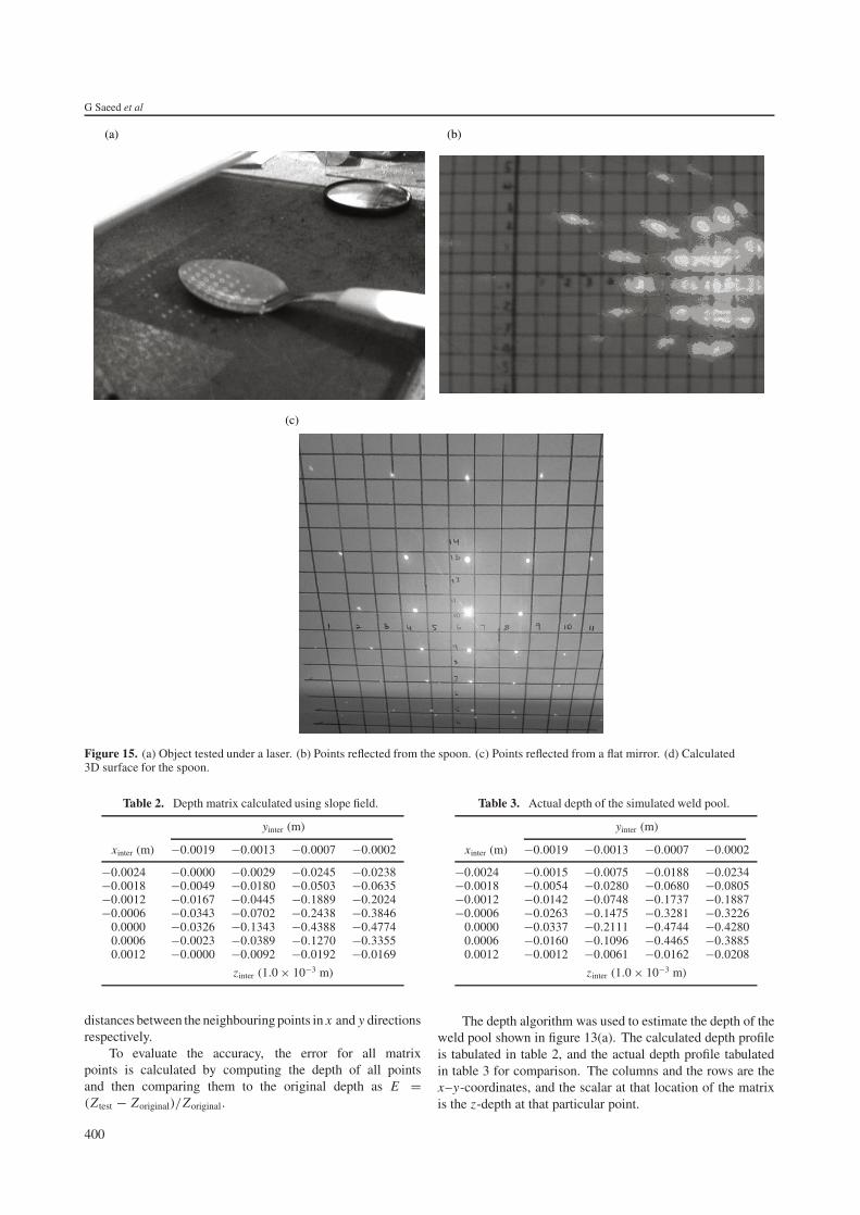
Figure 15. (a) Object tested under a laser. (b) Points reflected from the spoon. (c) Points reflected from a flat mirror. (d) Calculated3D surface for the spoon.

Table 2. Depth matrix calculated using slope field.

yinter (m)

xinter (m) −0.0019 −0.0013 −0.0007 −0.0002

−0.0024 −0.0000 −0.0029 −0.0245 −0.0238−0.0018 −0.0049 −0.0180 −0.0503 −0.0635−0.0012 −0.0167 −0.0445 −0.1889 −0.2024−0.0006 −0.0343 −0.0702 −0.2438 −0.3846

0.0000 −0.0326 −0.1343 −0.4388 −0.47740.0006 −0.0023 −0.0389 −0.1270 −0.33550.0012 −0.0000 −0.0092 −0.0192 −0.0169

zinter (1.0 × 10−3 m)

distances between the neighbouring points in x and y directionsrespectively.

To evaluate the accuracy, the error for all matrixpoints is calculated by computing the depth of all pointsand then comparing them to the original depth as E =(Z test − Zoriginal)/Zoriginal.

Table 3. Actual depth of the simulated weld pool.

yinter (m)

xinter (m) −0.0019 −0.0013 −0.0007 −0.0002

−0.0024 −0.0015 −0.0075 −0.0188 −0.0234−0.0018 −0.0054 −0.0280 −0.0680 −0.0805−0.0012 −0.0142 −0.0748 −0.1737 −0.1887−0.0006 −0.0263 −0.1475 −0.3281 −0.3226

0.0000 −0.0337 −0.2111 −0.4744 −0.42800.0006 −0.0160 −0.1096 −0.4465 −0.38850.0012 −0.0012 −0.0061 −0.0162 −0.0208

zinter (1.0 × 10−3 m)

The depth algorithm was used to estimate the depth of theweld pool shown in figure 13(a). The calculated depth profileis tabulated in table 2, and the actual depth profile tabulatedin table 3 for comparison. The columns and the rows are thex–y-coordinates, and the scalar at that location of the matrixis the z-depth at that particular point.

400


(c)


For the weld pool surface, the innermost depth is thekey parameter for its control. There are two major factorscontributing to the error in calculating this key parameter.

(1) The projected structure light is a point matrix and theresultant slope field is discrete. Hence, the resultant3D surface shape cannot represent the continuous changein an actual 3D surface shape. In the above test, thesimulated approximate depth according to table 3 is4.7736 × 10−4 m, and the deepest intersection point fromtable 2 is −4.7438 × 10−4 m. The error is 0.63%.

(2) Since incident rays may not illuminate the deepest point onthe weld pool surface, the deepest intersection point mustbe lower than the deepest point on the actual weld poolsurface, min(Z inter) > min(Zwelding). In the weld poolsimulation, the deepest point on the weld pool should be−5.2863×10−4 m. Compared to the approximated result,the error is 9.7%.

Figure 14 shows the approximation results in comparisonwith the actual weld pool surface. In particular, figure 14(a)shows the actual weld pool surface made using the GUIsimulation. Figure 14(b) gives the approximated weld poolsurface from the 2D slope field. Figure 14(c) shows asuperposition of the above two. From figure 14(c), thedepth is almost the same between the actual 3D shape andthe approximated 3D shape. However, due to the aboveapproximation method, especially in x and y coordinates, theapproximated shape has a little distortion in x and y directions.

6.3. Sample test 1

Using the above method, the 3D surfaces of objects withspecular reflection can be measured using a laser. For example,a set of laser ray points can be projected onto a spoon

(figure 15(a)) and the reflected points (figure 15(b)) can becompared with the points reflected from a flat mirror surface(figure 15(c)). The optical flow and slope field can then becalculated. Finally, the 3D surface shape can be derived fromthe slope field (figure 15(d)).

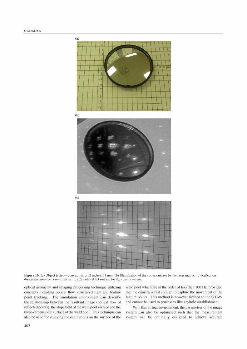
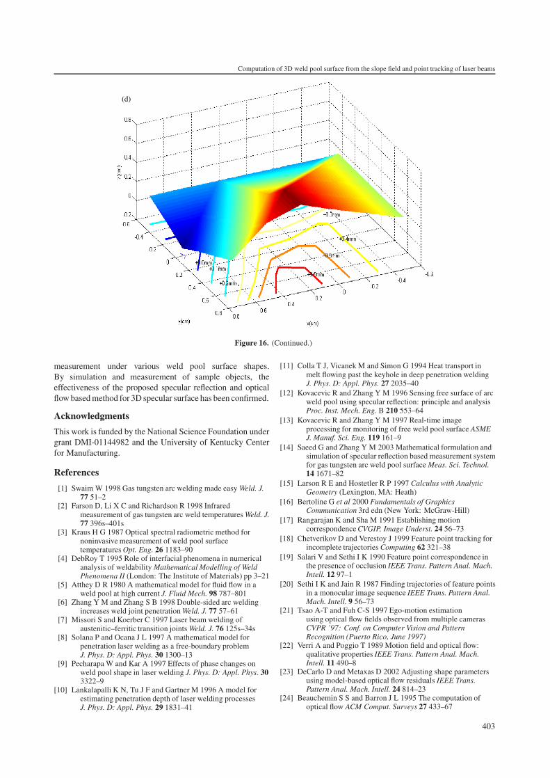
6.4. Sample test 2

In this example, a convex mirror surface is observed(figure 16(a)). To this end, a set of laser matrix points isprojected onto the mirror surface (figure 16(b)). The distortionof reflected laser points (figure 16(c)) is compared with thelaser points reflected from a flat mirror. Finally, the 3Dsurface is calculated from the slope field (figure 16(d)). Inthe calculated 3D surface, the maximum height is 0.6817 cm.The actual maximum height of the convex mirror surfaceis 0.680 59 cm. The actual height was measured using acoordinate measuring machine (CMM) at the meteorologylaboratory at the University of Kentucky. The error is only0.16%.

7. Conclusion

Monitoring of the free weld pool surface is an important issuefor studying and controlling welding processes. However,due to the strong arc and the mirror-like surface, limitedachievement has been made. The novel computation of the3D weld pool surface from specular reflection as proposedin this paper provides a solution. This paper summarizes theinitial research work which establishes the knowledge base andsimulation environment.

In particular, this paper has established the mathematicalmodel for the three-dimensional surface measurementmechanism, and has set up a simulation environment based on

401

G Saeed et al

(a)

(b)

(c)

Figure 16. (a) Object tested—convex mirror, 2 inches/51 mm. (b) Illumination of the convex mirror by the laser matrix. (c) Reflectiondistortion from the convex mirror. (d) Calculated 3D surface for the convex mirror.

optical geometry and imaging processing technique utilizingconcepts including optical flow, structured light and featurepoint tracking. The simulation environment can describethe relationship between the resultant image (optical flow ofreflected points), the slope field of the weld pool surface and thethree-dimensional surface of the weld pool. This technique canalso be used for studying the oscillations on the surface of the

weld pool which are in the order of less than 100 Hz, providedthat the camera is fast enough to capture the movement of thefeature points. This method is however limited to the GTAWand cannot be used in processes like keyhole establishment.

With this virtual environment, the parameters of the imagesystem can also be optimized such that the measurementsystem will be optimally designed to achieve accurate

402


(d)


measurement under various weld pool surface shapes.By simulation and measurement of sample objects, theeffectiveness of the proposed specular reflection and opticalflow based method for 3D specular surface has been confirmed.

Acknowledgments

This work is funded by the National Science Foundation undergrant DMI-01144982 and the University of Kentucky Centerfor Manufacturing.

References

[1] Swaim W 1998 Gas tungsten arc welding made easy Weld. J.77 51–2

[2] Farson D, Li X C and Richardson R 1998 Infraredmeasurement of gas tungsten arc weld temperatures Weld. J.77 396s–401s

[3] Kraus H G 1987 Optical spectral radiometric method fornoninvasive measurement of weld pool surfacetemperatures Opt. Eng. 26 1183–90

[4] DebRoy T 1995 Role of interfacial phenomena in numericalanalysis of weldability Mathematical Modelling of WeldPhenomena II (London: The Institute of Materials) pp 3–21

[5] Atthey D R 1980 A mathematical model for fluid flow in aweld pool at high current J. Fluid Mech. 98 787–801

[6] Zhang Y M and Zhang S B 1998 Double-sided arc weldingincreases weld joint penetration Weld. J. 77 57–61

[7] Missori S and Koerber C 1997 Laser beam welding ofaustenitic–ferritic transition joints Weld. J. 76 125s–34s

[8] Solana P and Ocana J L 1997 A mathematical model forpenetration laser welding as a free-boundary problemJ. Phys. D: Appl. Phys. 30 1300–13

[9] Pecharapa W and Kar A 1997 Effects of phase changes onweld pool shape in laser welding J. Phys. D: Appl. Phys. 303322–9

[10] Lankalapalli K N, Tu J F and Gartner M 1996 A model forestimating penetration depth of laser welding processesJ. Phys. D: Appl. Phys. 29 1831–41

[11] Colla T J, Vicanek M and Simon G 1994 Heat transport inmelt flowing past the keyhole in deep penetration weldingJ. Phys. D: Appl. Phys. 27 2035–40

[12] Kovacevic R and Zhang Y M 1996 Sensing free surface of arcweld pool using specular reflection: principle and analysisProc. Inst. Mech. Eng. B 210 553–64

[13] Kovacevic R and Zhang Y M 1997 Real-time imageprocessing for monitoring of free weld pool surface ASMEJ. Manuf. Sci. Eng. 119 161–9

[14] Saeed G and Zhang Y M 2003 Mathematical formulation andsimulation of specular reflection based measurement systemfor gas tungsten arc weld pool surface Meas. Sci. Technol.14 1671–82

[15] Larson R E and Hostetler R P 1997 Calculus with AnalyticGeometry (Lexington, MA: Heath)

[16] Bertoline G et al 2000 Fundamentals of GraphicsCommunication 3rd edn (New York: McGraw-Hill)

[17] Rangarajan K and Sha M 1991 Establishing motioncorrespondence CVGIP, Image Underst. 24 56–73

[18] Chetverikov D and Verestoy J 1999 Feature point tracking forincomplete trajectories Computing 62 321–38

[19] Salari V and Sethi I K 1990 Feature point correspondence inthe presence of occlusion IEEE Trans. Pattern Anal. Mach.Intell. 12 97–1

[20] Sethi I K and Jain R 1987 Finding trajectories of feature pointsin a monocular image sequence IEEE Trans. Pattern Anal.Mach. Intell. 9 56–73

[21] Tsao A-T and Fuh C-S 1997 Ego-motion estimationusing optical flow fields observed from multiple camerasCVPR ’97: Conf. on Computer Vision and PatternRecognition (Puerto Rico, June 1997)

[22] Verri A and Poggio T 1989 Motion field and optical flow:qualitative properties IEEE Trans. Pattern Anal. Mach.Intell. 11 490–8

[23] DeCarlo D and Metaxas D 2002 Adjusting shape parametersusing model-based optical flow residuals IEEE Trans.Pattern Anal. Mach. Intell. 24 814–23

[24] Beauchemin S S and Barron J L 1995 The computation ofoptical flow ACM Comput. Surveys 27 433–67

403

Computation of 3D weld pool surface from the slope field and point

Documents

Transcript of Computation of 3D weld pool surface from the slope field and point