COMPUTATIONAL LEARNING THEORY

Sally A� Goldman� Washington University� St� Louis Missouri

� Introduction

Since the late �fties� computer scientists �particularly those working in the area of arti�cial intel�

ligence� have been trying to understand how to construct computer programs that perform tasks

we normally think of as requiring human intelligence� and which can improve their performance

over time by modifying their behavior in response to experience� In other words� one objective

has been to design computer programs that can learn� For example� Samuels designed a program

to play checkers in the early sixties that could improve its performance as it gained experience

playing against human opponents� More recently� research on arti�cial neural networks has stim�

ulated interest in the design of systems capable of performing tasks that are di�cult to describe

algorithmically �such as recognizing a spoken word or identifying an object in a complex scene��

by exposure to many examples�

As a concrete example consider the task of hand�written character recognition� A learning

algorithm is given a set of examples where each contains a hand�written character as speci�ed

by a set of attributes �e�g� the height of the letter� along with the name �label� for the intended

character� This set of examples is often called the training data� The goal of the learner is to

e�ciently construct a rule �often referred to as a hypothesis or classi�er� that can be used to

take some previously unseen character and with high accuracy determine the proper label�

Computational learning theory is a branch of theoretical computer science that formally

studies how to design computer programs that are capable of learning� and identi�es the com�

putational limits of learning by machines� Historically� researchers in the arti�cial intelligence

community have judged learning algorithms empirically� according to their performance on sam�

ple problems� While such evaluations provide much useful information and insight� often it is hard

using such evaluations to make meaningful comparisons among competing learning algorithms�

Computational learning theory provides a formal framework in which to precisely formulate

and address questions regarding the performance of dierent learning algorithms so that careful

comparisons of both the predictive power and the computational e�ciency of alternative learning

algorithms can be made� Three key aspects that must be formalized are the way in which the

learner interacts with its environment� the de�nition of successfully completing the learning task�

and a formal de�nition of e�ciency of both data usage �sample complexity� and processing time

�time complexity�� It is important to remember that the theoretical learning models studied

are abstractions from real�life problems� Thus close connections with experimentalists are useful

to help validate or modify these abstractions so that the theoretical results help to explain or

predict empirical performance� In this direction� computational learning theory research has

close connections to machine learning research� In addition to its predictive capability� some

other important features of a good theoretical model are simplicity� robustness to variations in

the learning scenario� and an ability to create insights to empirically observed phenomena�

The �rst theoretical studies of machine learning were performed by inductive inference re�

searchers �see �Angluin and Smith� � ��� beginning with the introduction of the �rst formal

de�nition of learning given by �Gold� ����� In Gold�s model� the learner receives a sequence

of examples and is required to make a sequence of guesses as to the underlying rule �concept�

such that this sequence converges at some �nite point to a single guess that correctly names

the unknown rule� A key distinguishing characteristic is that Gold�s model does not attempt to

capture any notion of the e�ciency of the learning process whereas the �eld of computational

learning theory emphasizes the computational feasibility of the learning algorithm�

Another closely related �eld is that of pattern recognition �see �Duda and Hart� ���� and

�Devroye� Gy�or�� and Lugosi� ������ Much of the theory developed by learning theory researchers

to evaluate the amount of data needed to learn directly adapts results from the �elds of statistics

and pattern recognition� A key distinguishing factor is that learning theory researchers study

both the data �information� requirements for learning and the time complexity of the learning

algorithm� �In contrast� pattern recognition researchers tend to focus on issues related to the

data requirements�� Finally� there are a lot of close relations to work on arti�cial neural networks�

While much of neural network research is empirical� there is also a good amount of theoretical

�

work �see �Devroye� Gy�or�� and Lugosi� ������

This chapter is structured as follows� In Section � we describe the basic framework of concept

learning and give notation that we use throughout the chapter� Next� in Section � we describe the

PAC �distribution�free� model that began the �eld of computational learning theory� An impor�

tant early result in the �eld is the demonstration of the relationships between the VC�dimension�

a combinatorial measure� and the data requirements for PAC learning� We then discuss some

commonly studied noise models and general techniques for PAC learning from noisy data�

In Section � we cover some of the other commonly studied formal learning models� In Sec�

tion �� we study an on�line learning model� Unlike the PAC model in which there is a training

period� in the on�line learning model the learner must improve the quality of its predictions as it

functions in the world� Next� in Section ���� we study the query model which is very similar to

the on�line model except that the learner plays a more active role�

As in other theoretical �elds� along with having techniques to prove positive results� another

important component of learning theory research is to develop and apply methods to prove when

a learning problem is hard� In Section � we describe some techniques used to show that learning

problems are hard� Next� in Section �� we explore a variation of the PAC model called the

weak learning model� and study techniques for boosting the performance of a mediocre learning

algorithm� Finally� we close with a brief overview of some of the many current research issues

being studied within the �eld of computational learning theory�

� General Framework

For ease of exposition� we initially focus on concept learning in which the learner�s goal is to infer

how an unknown target function classi�es �as positive or negative� examples from a given domain�

In the character recognition example� one possible task of the learner would be to classify each

character as a numeral or non�numeral� Most of the de�nitions given here naturally extend to

the general setting of learning functions with multiple�valued or real�valued outputs� Later in

Section �� we brie�y discuss the more general problem of learning a real�valued function�

�

...

Figure �� The left �gure shows �in ��� a concept from Chalfspace and the right �gure shows a

concept for C�shalfspace for s � �� The points from �� that are classi�ed as positive are shaded�

The unshaded points are classi�ed as negative�

��� Notation

The instance space �domain� X is the set of all possible objects �instances� to be classi�ed� Two

very common domains are the boolean hypercube f�� gn� and the continuous n�dimensional

space �n� For example� if there are n boolean attributes then each example can be expressed as

an element of f�� gn� Likewise� if there are n real�valued attributes� then �n can be used� A

concept f is a boolean function over domain X � Each x � X is referred to as an example �point��

A concept class C is a collection of subsets of X � That is C � �X � Typically �but not always��

it is assumed that the learner has prior knowledge of C� Examples are classi�ed according to

membership of a target concept f � C� Often� instead of using this set theoretic view of C� a

functional view is used in which f�x� gives the classi�cation of concept f � C for each example

x � X � An example x � X is a positive example of f if f�x� � �equivalently x � f�� or a

negative example of f if f�x� � � �or equivalently x �� f�� Often C is decomposed into subclasses

Cn according to some natural size measure n for encoding an example� For example� in the

boolean domain� n is the number of boolean attributes� Let Xn denote the set of examples to be

classi�ed for each problem of size n� X �Sn�� Xn�

We use the class Chalfspace� the set of halfspaces in �n� and the class C�shalfspace� the set of all the

intersections of up to s halfspaces in �d� to illustrate some of the basic techniques for designing

�

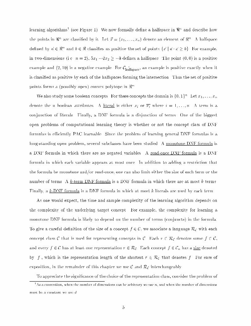
learning algorithms� �see Figure �� We now formally de�ne a halfspace in �n and describe how

the points in �n are classi�ed by it� Let �x � �x�� � � � � xn� denote an element of �n� A halfspace

de�ned by �a � �n and b � � classi�es as positive the set of points f�x j �a � �x � bg� For example�

in two�dimensions �i�e� n � ��� �x�� �x� � �� de�nes a halfspace� The point ��� �� is a positive

example and ��� �� is a negative example� For C�shalfspace� an example is positive exactly when it

is classi�ed as positive by each of the halfspaces forming the intersection� Thus the set of positive

points forms a �possibly open� convex polytope in �n�

We also study some boolean concepts� For these concepts the domain is f�� gn� Let x�� � � � � xn

denote the n boolean attributes� A literal is either xi or xi where i � � � � � � n� A term is a

conjunction of literals� Finally� a DNF formula is a disjunction of terms� One of the biggest

open problems of computational learning theory is whether or not the concept class of DNF

formulas is e�ciently PAC learnable� Since the problem of learning general DNF formulas is a

long�standing open problem� several subclasses have been studied� A monotone DNF formula is

a DNF formula in which there are no negated variables� A read�once DNF formula is a DNF

formula in which each variable appears at most once� In addition to adding a restriction that

the formula be monotone and�or read�once� one can also limit either the size of each term or the

number of terms� A k�term DNF formula is a DNF formula in which there are at most k terms�

Finally� a k�DNF formula is a DNF formula in which at most k literals are used by each term�

As one would expect� the time and sample complexity of the learning algorithm depends on

the complexity of the underlying target concept� For example� the complexity for learning a

monotone DNF formula is likely to depend on the number of terms �conjuncts� in the formula�

To give a careful de�nition of the size of a concept f � C� we associate a language RC with each

concept class C that is used for representing concepts in C� Each r � RC denotes some f � C�

and every f � C has at least one representation r � RC� Each concept f � Cn has a size denoted

by jf j� which is the representation length of the shortest r � RC that denotes f � For ease of

exposition� in the remainder of this chapter we use C and RC interchangeably�

To appreciate the signi�cance of the choice of the representation class� consider the problem of

�As a convention� when the number of dimensions can be arbitrary we use n� and when the number of dimensions

must be a constant we use d�

�

learning a regular language�� The question as to whether an algorithm is e�cient depends heavily

on the representation class� As de�ned more formally below� an e�cient learning algorithm must

have time and sample complexity polynomial in jf j where f is the target concept� The target

regular language could be represented as a deterministic �nite�state automaton �DFA� or as

a non�deterministic �nite�state automaton �NFA�� However� the length of the representation

as a NFA can be exponentially smaller than the shortest representation as a DFA� Thus� the

learner may be allowed exponentially more time when learning the class of regular languages as

represented by DFAs versus when learning the class of regular languages as represented by NFAs�

Often to make the representation class clear� the concept class names the representation� Thus

instead of talking about learning a regular language� we talk about learning a DFA or an NFA�

Thus the problem of learning a DFA is easier than learning an NFA� Similar issues arise when

learning boolean functions� For example� whether the function is represented as a decision tree�

a DNF formula� or a boolean circuit greatly aects the representation size�

� PAC Learning Model

The �eld of computational learning theory began with Valiant�s seminal work �Valiant� � ��

in which he de�ned the PAC��distribution�free� learning model� In the PAC model examples

are generated according to an unknown probability distribution D� and the goal of a learning

algorithm is to classify with high accuracy �with respect to the distribution D� any further

�unclassi�ed� examples�

We now formally de�ne the PAC model� To obtain information about an unknown target

function f � Cn� the learner is provided access to labeled �positive and negative� examples of

f � drawn randomly according to some unknown target distribution D over Xn� The learner is

also given as input � and � such that � � �� � � � and an upper bound k on jf j� The learner�s

goal is to output� with probability at least � �� a hypothesis h � Cn that has probability at

�See Section ��� of Chapter �� and Section � of Chapter �� in this handbook for background on regular

languages� DFAs and NFAs�

�PAC is an acronym coined by Dana Angluin for probably approximately correct�

�

most � of disagreeing with f on a randomly drawn example from D �thus� h has error at most

��� If such a learning algorithm A exists �that is� an algorithm A meeting the goal for any n � �

any target concept f � Cn� any target distribution D� any �� � � �� and any k � jf j�� then C

is PAC learnable� A PAC learning algorithm is a polynomial�time �e�cient� algorithm if the

number of examples drawn and the computation time are polynomial in n� k� �� and �� We

note that most learning algorithms are really functions from samples to hypotheses �i�e� given a

sample S the learning algorithm produces a hypothesis h�� It is only for the analysis in which

we say that for a given � and �� the learning algorithm is guaranteed with probability at least

� � to output a hypothesis with error at most � given a sample whose size is a function of �� ��

n and k� Thus� empirically� one can generally run a PAC algorithm on provided data and then

empirically measure the error of the �nal hypothesis� One exception is when trying to empirically

use statistical query algorithms since� for most of these algorithms� the algorithm uses � for more

than just determining the desired sample size� �See Section ��� for a discussion of statistical

query algorithms� and �Goldman and Scott� ���� for a discussion of their empirical use��

As originally formulated� PAC learnability also required the hypothesis to be a member of

the concept class Cn� We refer to this more stringent learning model as proper PAC�learnability�

The work of �Pitt and Valiant� � � shows that a prerequisite for proper PAC�learning is the

ability to solve the consistent hypothesis problem� which is the problem of �nding a concept

f � C that is consistent with a provided sample� Their result implies that if the consistent

hypothesis problem is NP�hard for a given concept class �as they show is the case for the class of

k�term DNF formulas� and NP �� RP� then the learning problem is hard�� A more general form

of learning in which the goal is to �nd any polynomial�time algorithm that classi�es instances

accurately in the PAC sense is commonly called prediction� In this less stringent variation of the

PAC model� the algorithm need not output a hypothesis from the concept class C but instead

is just required to make its prediction in polynomial time� This idea of prediction in the PAC

model originated in the paper of �Haussler� Littlestone� and Warmuth� ����� and is discussed

in �Pitt and Warmuth� ����� Throughout the remainder of this chapter� when referring to the

�For background on Complexity Classes see Chapter �� �NP dened and Chapter ��� Section � �RP dened

of this handbook�

�

PAC learning model we allow the learner to output any hypothesis that can be evaluated in

polynomial time� That is� given a hypothesis h and an example x� we require that h�x� can be

computed in polynomial time� We refer to the model in which the learner is required to output

a hypothesis h � Cn as the proper PAC learning model�

Many variations of the PAC model are known to be equivalent �in terms of what concept

classes are e�ciently learnable� to the model de�ned above� We now brie�y discuss one of

these variations� In the above de�nition of the PAC model� along with receiving �� �� and n

as input� the learner also receives k� an upperbound on jf j� The learner must be given � and

�� Further� by looking at just one example� the value of n is known� Yet giving the learner

knowledge of k may appear to make the problem easier� However� if the demand of polynomial�

time computation is replaced with expected polynomial�time computation� then the learning

algorithm need not be given the parameter k� but could �guess� it instead� We now brie�y

review the standard doubling technique used to convert an algorithm A designed to have k as

input to an algorithm B that has no prior knowledge of k� Algorithm B begins with an estimate�

say � for its upperbound on k and runs algorithm A using this estimate to obtain hypothesis

h� Then algorithm B uses a hypothesis testing procedure to determine if the error of h is at

most �� Since the learner can only gather a random sample of examples� it is not possible

to distinguish a hypothesis with error � from one with error just greater than �� However�

by drawing a su�ciently large sample and looking at the empirical performance of h on that

sample� we can distinguish a hypothesis with error at most �� from one with error more than

�� In particular� given a sample� of size m �l��� ln �

�

m� if h misclassi�es at most ��

� �m examples

then B accepts h� Otherwise� algorithm B doubles its estimate for k and repeats the process�

For the technical details of the above argument as well as for a discussion the other equivalences�

see �Haussler� Kearns� Littlestone� and Warmuth� ����

�Cherno� bounds are used to compute the sample size so that the hypothesis testing procedure gives the desired

output with high probability�

+

-

-

++

++

+ -+

+-

+

--+

--

-- -

++

-

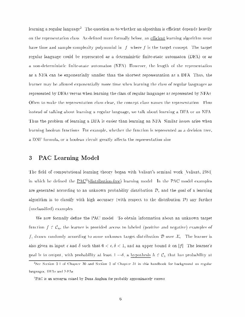
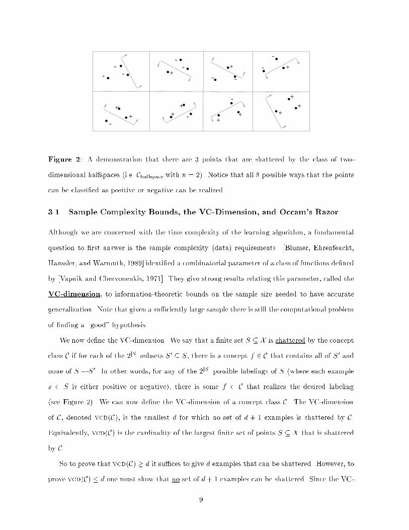
Figure �� A demonstration that there are � points that are shattered by the class of two�

dimensional halfspaces �i�e� Chalfspace with n � ��� Notice that all possible ways that the points

can be classi�ed as positive or negative can be realized�

��� Sample Complexity Bounds� the VC�Dimension� and Occam�s Razor

Although we are concerned with the time complexity of the learning algorithm� a fundamental

question to �rst answer is the sample complexity �data� requirements� �Blumer� Ehrenfeucht�

Haussler� and Warmuth� � �� identi�ed a combinatorial parameter of a class of functions de�ned

by �Vapnik and Chervonenkis� ���� They give strong results relating this parameter� called the

VC�dimension� to information�theoretic bounds on the sample size needed to have accurate

generalization� Note that given a su�ciently large sample there is still the computational problem

of �nding a �good� hypothesis�

We now de�ne the VC�dimension� We say that a �nite set S � X is shattered by the concept

class C if for each of the �jSj subsets S� � S� there is a concept f � C that contains all of S� and

none of S � S�� In other words� for any of the �jSj possible labelings of S �where each example

s � S is either positive or negative�� there is some f � C that realizes the desired labeling

�see Figure ��� We can now de�ne the VC�dimension of a concept class C� The VC�dimension

of C� denoted vcd�C�� is the smallest d for which no set of d � examples is shattered by C�

Equivalently� vcd�C� is the cardinality of the largest �nite set of points S � X that is shattered

by C�

So to prove that vcd�C� � d it su�ces to give d examples that can be shattered� However� to

prove vcd�C� � d one must show that no set of d� examples can be shattered� Since the VC�

�

dimension is so fundamental in determining the sample complexity required for PAC learning�

we now go through several sample computations of the VC�dimension�

Axis�parallel rectangles in ��� For this concept class the points lying on or inside the target

rectangle are positive� and points lying outside the target rectangle are negative� First� it

is easily seen that there is a set of four points �e�g� f��� �� ������ �� ��� ��� ��g� that can

be shattered� Thus vcd�C� � �� We now argue that no set of �ve points can be shattered�

The smallest bounding axis�parallel rectangle de�ned by the �ve points is in fact de�ned by

at most four of the points� For p a non�de�ning point in the set� we see that the set cannot

be shattered since it is not possible for p to be classi�ed as negative while also classifying

the others as positive� Thus vcd�C� � ��

Halfspaces in ��� Points lying in or on the halfspace are positive� and the remaining points are

negative� It is easily shown that any three non�collinear points �e�g� ��� �� ��� ��� �� ��� are

shattered by C �recall Figure ��� Thus vcd�C� � �� We now show that no set of size four

can be shattered by C� If at least three of the points are collinear then there is no halfspace

that contains the two extreme points but does not contain the middle points� Thus the four

points cannot be shattered if any three are collinear� Next� suppose that the points form

a quadrilateral� There is no halfspace which labels one pair of diagonally opposite points

positive and the other pair of diagonally opposite points negative� The �nal case is that

one point p is in the triangle de�ned by the other three� In this case there is no halfspace

which labels p dierently from the other three� Thus clearly the four points cannot be

shattered� Therefore we have demonstrated that vcd�C� � �� Generalizing to halfspaces

in �n� it can be shown that vcd�Chalfspace� � n � �see �Blumer� Ehrenfeucht� Haussler�

and Warmuth� � ����

Closed sets in ��� All points lying in the set or on the boundary of the set are positive� and

all points lying outside the set are negative� Any set can be shattered by C� since a closed

set can assume any shape in ��� Thus� the largest set that can be shattered by C is in�nite�

and hence vcd�C� � �

�

We now brie�y discuss techniques that aid in computing the VC�dimension of more complex

concept classes� Suppose we wanted to compute the VC�dimension of C�shalfspace� the class of

intersections of up to s halfspaces over �d� We would like to make use of our knowledge of the

VC�dimension of Chalfspace� the class of halfspaces over �d� �Blumer� Ehrenfeucht� Haussler� and

Warmuth� � �� gave the following result� let C be a concept class with vcd�C� � D� Then the

class de�ned by the intersection of up to s concepts from C has VC�dimension� at most �Ds lg��s��

In fact� the above result applies when replacing intersection with any boolean function� Thus

the concept class C�shalfspace �where each halfspace is de�ned over �d� has VC�dimension at most

��d� �s lg��s��

We now discuss the signi�cance of the VC�dimension to the PAC model� One important

property is that for D � vcd�C�� the number of dierent labelings that can be realized �also

referred to as behaviors� using C for a set S is at most�ejSjD

�D� Thus for a constant D we

have polynomial growth in the number of labelings versus the exponential growth of �jSj� A key

result in the PAC model is that of �Blumer� Ehrenfeucht� Haussler� and Warmuth� � �� that

gives an upperbound on the sample complexity needed to PAC learn in terms of �� �� and the

VC�dimension of the hypothesis class� They proved that one can design a learning algorithm

A for concept class C using hypothesis space H in the following manner� Any concept h � H

consistent with a sample of size max��� lg

�� �

�vcd�H� lg ��

�

�has error at most � with probability

at least � �� To obtain a polynomial�time PAC learning algorithm what remains is to solve

the algorithmic problem of �nding a hypothesis from H consistent with the labeled sample�

Furthermore� �Ehrenfeucht and Haussler� � �� proved an information�theoretic lower bound that

learning any concept class C requires ���� log

�� � vcd�C

�

�examples in the worst case� As an

example application� see Figure ��

A key limitation of this technique to design a PAC learning algorithm is that the hypothesis

must be drawn from some �xed hypothesis classH� In particular� the complexity of the hypothesis

class must be independent of the sample size� However� often the algorithmic problem of �nding

such a hypothesis from the desired class is NP�hard�

�Note that throughout this chapter� lg is used for the base � logarithm� When the base of the logarithm is not

signicant �such as when using asymptotic notation� we use log�

PAC�learn�halfspace�n� �� ��

Draw a labeled sample S of size max���lg �

�� � �n���

�lg ��

�

�Use a polynomial�time linear programming algorithm to �nd a halfspace h consistent with SOutput h

Figure �� A PAC algorithm to learn a concept from Chalfspace� Recall that vcd�Chalfspace� � n��

As an example suppose we tried to modify PAC�learn�halfspace from Figure � to e�ciently

PAC learn the class of intersections of at most s halfspaces in �d for d the number of dimensions

a constant� Suppose we are given a sample S of m example points labeled according to some

f � C�shalfspace� The algorithmic problem of �nding a hypothesis from C�shalfspace can be formulated

as a set covering problem in the following manner� An instance of the set covering problem is a

set U and a family T of subsets of U such that �St�T t� � U � A solution is a smallest cardinality

subset G of T such that�S

g�G g�

� U � Consider any halfspace g that correctly classi�es all

positive examples from S� We say that g covers all of the negative examples from S that are

also classi�ed as negative by g� Thus U is the set of negative examples from S� and T is the set

of representative halfspaces �one for each behavior with respect to S� that correctly classify all

positive examples from S�

So �nding a minimum sized hypothesis from C�shalfspace consistent with the sample S is exactly

the problem of �nding the minimum number of halfspaces that are required to cover all negative

points in S� Given that the set covering problem is NP�complete� how can we proceed We

can apply the greedy approximation algorithm that has a ratio bound of ln jUj � to �nd a

hypothesis consistent with S that is the intersection of at most ln jSj� halfspaces� However�

since the VC�dimension of the hypothesis grows with the size of the sample� the basic technique

described above cannot be applied� In general� when using a set covering approach� the size of

the hypothesis often depends on the size of the sample�

�Blumer� Ehrenfeucht� Haussler� and Warmuth� � � and � �� extended this basic tech�

nique by showing that �nding a hypothesis h consistent with a sample S for which the size

of h is sub�linear in jSj is su�cient to guarantee PAC learnability� In other words� by ob�

taining su�cient data compression one obtains good generalization� More formally� let HAk�n�m

�

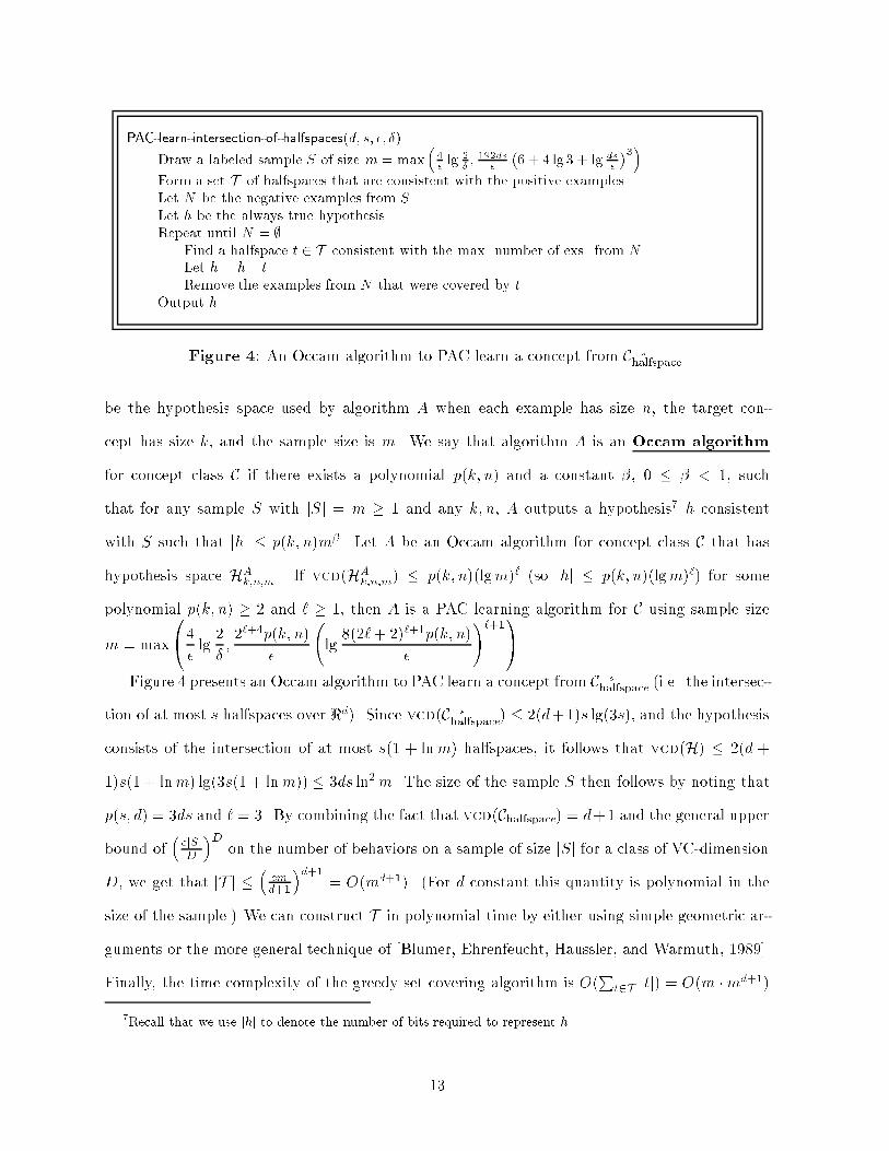
PAC�learn�intersection�of�halfspaces�d� s� �� ��

Draw a labeled sample S of size m � max���lg �

�� ��ds

�

�� � � lg � lg ds

�

���Form a set T of halfspaces that are consistent with the positive examplesLet N be the negative examples from SLet h be the always true hypothesisRepeat until N � �

Find a halfspace t � T consistent with the max number of exs from NLet h � h � tRemove the examples from N that were covered by t

Output h

Figure �� An Occam algorithm to PAC learn a concept from C�shalfspace�

be the hypothesis space used by algorithm A when each example has size n� the target con�

cept has size k� and the sample size is m� We say that algorithm A is an Occam algorithm

for concept class C if there exists a polynomial p�k� n� and a constant � � � � � such

that for any sample S with jSj � m � and any k� n� A outputs a hypothesis h consistent

with S such that jhj � p�k� n�m�� Let A be an Occam algorithm for concept class C that has

hypothesis space HAk�n�m� If vcd�HA

k�n�m� � p�k� n��lgm�� �so jhj � p�k� n��lgm��� for some

polynomial p�k� n� � � and � � � then A is a PAC learning algorithm for C using sample size

m � max

���

�lg

�

������p�k� n�

�

�lg

���� �����p�k� n�

�

���A�

Figure � presents an Occam algorithm to PAC learn a concept from C�shalfspace �i�e� the intersec�

tion of at most s halfspaces over �d�� Since vcd�C�shalfspace� � ��d��s lg��s�� and the hypothesis

consists of the intersection of at most s� � lnm� halfspaces� it follows that vcd�H� � ��d �

�s� � lnm� lg��s� � lnm�� � �ds ln�m� The size of the sample S then follows by noting that

p�s� d� � �ds and � � �� By combining the fact that vcd�Chalfspace� � d� and the general upper

bound of�ejSjD

�Don the number of behaviors on a sample of size jSj for a class of VC�dimension

D� we get that jT j ��emd��

�d��� O�md���� �For d constant this quantity is polynomial in the

size of the sample�� We can construct T in polynomial time by either using simple geometric ar�

guments or the more general technique of �Blumer� Ehrenfeucht� Haussler� and Warmuth� � ���

Finally� the time complexity of the greedy set covering algorithm is O�P

t�T jtj� � O�m �md���

�Recall that we use jhj to denote the number of bits required to represent h�

�

which is polynomial in s �the number of halfspaces�� �� and � for d �the number of dimensions�

constant�

For the problem of learning the intersection of halfspaces the greedy covering technique pro�

vided substantial data compression� Namely� the size of our hypothesis only had a logarithmic

dependence on the size of the sample� In general� only a sub�linear dependence is required as

given by the following result of �Blumer� Ehrenfeucht� Haussler� and Warmuth� � ��� Let A be

an Occam algorithm for concept class C that has hypothesis space HAk�n�m� If vcd�HypAk�n�m� �

p�k� n�m� �so jhj � p�k� n�m�� for some polynomial p�k� n� � � and � � then A is a PAC

learning algorithm for C using sample size m � max

��

�ln

��

�� ln �

�� p�k� n�

� ����

�

��� Models of Noise

The basic de�nition of PAC learning assumes that the data received is drawn randomly from

D and properly labeled according to the target concept� Clearly� for learning algorithms to be

of practical use they most be robust to noise in the training data� In order to theoretically

study an algorithm�s tolerance to noise� several formal models of noise have been studied� In

the model of Random Classi�cation Noise��Angluin and Laird� � �� with probability � ��

the learner receives the uncorrupted example �x� ��� However� with probability �� the learner

receives the example �x� !��� So in this noise model� learner usually gets a correct example� but

some small fraction � of the time the learner receives an example in which the label has been

inverted� In the model of Malicious Classi�cation Noise��Sloan� � �� with probability ��� the

learner receives the uncorrupted example �x� ��� However� with probability �� the learner receives

the example �x� ��� in which x is unchanged� but the label �� is selected by an adversary who

has in�nite computing power and has knowledge of the learning algorithm� the target concept�

and the distribution D� In the previous two models� only the labels are corrupted� Another

noise model is that of Malicious Noise��Valiant� � ���� In this model� with probability � ��

the learner receives the uncorrupted example �x� ��� However� with probability �� the learner

receives an example �x�� ��� about which no assumptions whatsoever may be made� In particular�

this example �and its label� may be maliciously selected by an adversary� Thus in this model�

the learner usually gets a correct example� but some small fraction � of the time the learner gets

�

noisy examples and the nature of the noise is unknown�

We now de�ne two noise models that are only de�ned when the instance space is f�� gn�

In the model of Uniform Random Attribute Noise ��Sloan� � ��� the example �b� � � �bn� �� is

corrupted by a random process that independently �ips each bit bi to !bi with probability � for

� i � n� Note that the label of the �true� example is never altered� In this noise model� the

attributes� values are subject to noise� but that noise is as benign as possible� For example� the

attributes� values might be sent over a noisy channel� but the label is not� Finally� in the model of

Product Random Attribute Noise��Goldman and Sloan� ������ the example �b� � � �bn� �� is cor�

rupted by a random process of independently �ipping each bit bi to !bi with some �xed probability

�i � � for each � i � n� Thus unlike the model of uniform random attribute noise� the noise

rate associated with each bit of the example may be dierent�

��� Gaining Noise Tolerance in the PAC Model

Some of the �rst work on designing noise�tolerant PAC algorithms was done by �Angluin and

Laird� � �� They gave an algorithm for learning boolean conjunctions that tolerates random

classi�cation noise of a rate approaching the information�theoretic barrier of �� Furthermore�

they proved that the general technique of �nding a hypothesis that minimizes disagreements with

a su�ciently large sample allows one to handle random classi�cation noise of any rate approaching

�� However� they showed that even the very simple problem of minimizing disagreements �when

there are no assumptions about the noise� is NP�hard� Until recently� there have been a small

number of e�cient noise�tolerant PAC algorithms� but no general techniques were available to

design such algorithms� and there was little work to characterize which concept classes could be

e�ciently learned in the presence of noise�

The �rst �computationally feasible� tool to design noise�tolerant PAC algorithms was pro�

vided by the statistical query model� �rst introduced by �Kearns� ����� and since improved

by �Aslam and Decatur� ����� In this model� rather than sampling labeled examples� the

learner requests the value of various statistics� A relative�error statistical query �Aslam and

Decatur� ���� takes the form SQ� � �� �� where is a predicate over labeled examples� � is a

relative error bound� and � is a threshold� As an example� let to be ��h�x� � � �� � ���

�

which is true when x is a negative example but the hypothesis classi�es x as positive� So the

probability that is true for a random example is the false positive error of hypothesis h� For

target concept f � we de�ne P� � PrD � �x� f�x��� � � where PrD is used to denote that x is

drawn at random from distribution D� If P� � � then SQ� � �� �� may return �� If � is not re�

turned� then SQ� � �� �� must return an estimate "P� such that P����� � "P� � P������ The

learner may also request unlabeled examples �since we are only concerned about classi�cation

noise��

Let�s take our algorithm� PAC�learn�intersection�of�halfspaces and reformulate it as a relative�

error statistical query algorithm� First we draw an unlabeled sample Su that we use to generate

the set T of halfspaces to use for our covering� Similar to before� we place a halfspace in T

corresponding to each possible way in which the points of Su can be divided� Recall that before�

we only place a halfspace in T if it properly labeled the positive examples� Since we have an

unlabeled sample we cannot use such an approach� Instead� we use a statistical query �for each

potential halfspace� to check if a given halfspace is consistent with most of the positive examples�

Finally� when performing the greedy covering step we cannot pick the halfspace that covers the

most negative examples� but rather the one that covers the �most� �based on our empirical

estimate� negative weight� Figure � shows our algorithm in more depth�

We now cover the key ideas in proving that SQ�learn�intersection�of�halfspaces is correct� First�

we pick Su so that any hypothesis consistent with Su �if we knew the labels� would have error

at most ��r with probability � �

� � Since our hypothesis class is C�rhalfspace� and vcd�C�rhalfspace� �

��d� �r lg��r�� we obtain the sample size for Su�

For each of the s halfspaces that form the target concept� there is some halfspace in T

consistent with that halfspace over Su� and thus that has error at most ���r� on the positive

region� For each such halfspace t our estimate "P� �for the probability that t�x� � � and � � �

is at most ��r �

�� � �

�r � Thus� we place s halfspaces in Tgood that produce a hypothesis with false

negative error � ���r�� Let ei � Pr�h�x� � � � �� �i�e� the false positive error� after i rounds

of the while loop� Since ei is our current error and ���r� is a lower bound on the error we could

�

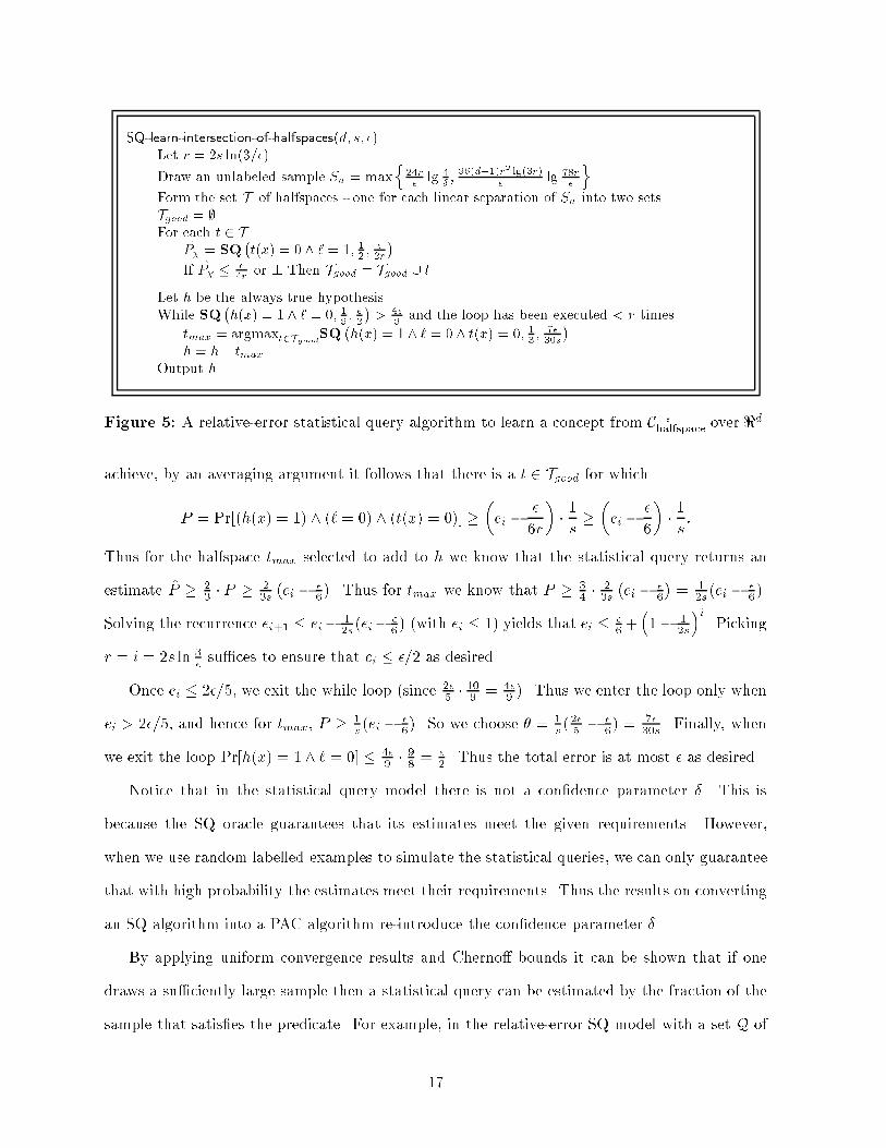
SQ�learn�intersection�of�halfspaces�d� s� ��Let r � �s ln����

Draw an unlabeled sample Su � maxn

��r�lg �

�� �d���r� lg��r�

�lg ��r

�

oForm the set T of halfspaces � one for each linear separation of Su into two setsTgood � �For each t � T

�P� � SQ�t�x� � � � � �� �� �

��r

�If �P� �

��r or � Then Tgood � Tgood � t

Let h be the always true hypothesisWhile SQ

�h�x� � � � � � � � �

��

�� ��

and the loop has been executed � r times

tmax � argmaxt�TgoodSQ�h�x� � � � � � � t�x� � � �� �

����s

�h � h � tmax

Output h

Figure � A relative�error statistical query algorithm to learn a concept from C�shalfspace over �d�

achieve� by an averaging argument it follows that there is a t � Tgood for which

P � Pr��h�x� � � �� � �� �t�x� � ��� �

�ei �

�

�r

��

s�

�ei �

�

�

��

s�

Thus for the halfspace tmax selected to add to h we know that the statistical query returns an

estimate "P � �� � P � �

�s

�ei �

��

�� Thus for tmax we know that P � �

� ���s

�ei �

��

�� �

�s�ei �����

Solving the recurrence ei�� � ei���s�ei�

��� �with ei � � yields that ei �

�� �

�� �

�s

�i� Picking

r � i � �s ln �� su�ces to ensure that ei � �� as desired�

Once ei � ���� we exit the while loop �since ��� �

�� � ��

�� Thus we enter the loop only when

ei � ���� and hence for tmax� P � �s �ei �

���� So we choose � � �

s ���� �

��� �

���s � Finally� when

we exit the loop Pr�h�x� � � � �� � �� �

� � �

� � Thus the total error is at most � as desired�

Notice that in the statistical query model there is not a con�dence parameter �� This is

because the SQ oracle guarantees that its estimates meet the given requirements� However�

when we use random labelled examples to simulate the statistical queries� we can only guarantee

that with high probability the estimates meet their requirements� Thus the results on converting

an SQ algorithm into a PAC algorithm re�introduce the con�dence parameter ��

By applying uniform convergence results and Cherno bounds it can be shown that if one

draws a su�ciently large sample then a statistical query can be estimated by the fraction of the

sample that satis�es the predicate� For example� in the relative�error SQ model with a set Q of

�

possible queries� �Aslam and Decatur� ���� show that a sample of size O�

��� log

jQj�

�su�ces to

appropriately answer � � �� �� for every � Q with probability at least � �� �If vcd�Q� � q

then a sample of size O�

q�� log

�� � �

�� log��

�su�ces��

To handle random classi�cation noise of any rate approaching � more complex methods

are used for answering the statistical queries� Roughly� using knowledge of the noise process

and a su�ciently accurate estimate of the noise rate �which must itself be determined by the

algorithm�� the noise process can be �inverted�� The total sample complexity required to simulate

an SQ algorithm in the presence of classi�cation noise of rate � � �b is #O�

log�jQj�����������b�

�where

�� �respectively� ��� is the minimum value of � �respectively� �� across all queries and � �

���� �� The soft�oh notation � #O� is similar to the standard big�oh notation except dominate

log factors are also removed� Alternatively� for the query space Q� the sample complexity is

O�

vcd�Q�����������b�

hlog

��

����������b

�� log �

�

i�� Notice that the amount by which �b is less than

� is just �����b

� �����b

� Thus the above are polynomial as long as �� � �b is at least one over

a polynomial�

� Exact and Mistake Bounded Learning Models

The PAC learning model is a batch model$there is a separation between the training phase and

the performance phase� In the training phase the learner is presented with labeled examples $

no predictions are expected� Then at the end of the training phase the learner must output

a hypothesis h to classify unseen examples� Also� since the learner never �nds out the true

classi�cation for the unlabeled instances� all learning occurs in the training phase� In many

settings� the learner does not have the luxury of a training phase but rather must learn as it

performs� We now study two closely related learning models designed for such a setting�

��� On�line Learning Model

To motivate the on�line learning model �also known as the mistake�bounded learning model��

suppose that when arriving at work �in Boston� you may either park in the street or park in

a garage� In fact� between your o�ce building and the garage there is a street on which you

can always �nd a spot� On most days� street parking is preferable since you avoid paying the

%� garage fee� Unfortunately� when parking on the street you risk being towed �%��� due to

street cleaning� snow emergency� special events� etc� When calling the city to �nd out when they

tow� you are unable to get any reasonable guidance and decide the best thing to do is just learn

from experience� There are many pieces of information that you might consider in making your

prediction� e�g� the date� the day of the week� the weather� We make the following assumption�

after you commit yourself to one choice or the other you learn of the right decision� In this

example� the city has rules dictating when they tow& you just don�t know them� If you park on

the street� at the end of the day you know if your car was towed& otherwise when walking to the

garage you see if the street is clear �i�e� you learn if you would have been towed�� The on�line

model is designed to study algorithms for learning to make accurate predictions in circumstances

such as these� Note that unlike the problems addressed by many techniques from reinforcement

learning� here there is immediate �versus delayed� feedback�

We now de�ne the on�line learning model for the general setting in which the target function

has a real�valued output �without loss of generality� scaled to be between � and �� An on�line

learning algorithm for C is an algorithm that runs under the following scenario� A learning session

consists of a set of trials� In each trial� the learner is given an unlabeled instance x � X � The

learner uses its current hypothesis to predict a value p�x� for the unknown �real�valued� target

concept f � C and then the learner is told the correct value for f�x�� Several loss functions have

been considered to measure the quality of the learner�s predictions� Three commonly used loss

functions are the following� the square loss de�ned by ���p�x�� f�x�� � �f�x��p�x���� the log loss

de�ned by �log�p�x�� f�x�� � �f�x� log p�x����f�x�� log��p�x��� and the absolute loss de�ned

by ���p�x�� f�x�� � jf�x�� p�x�j�

The goal of the learner is to make predictions so that total loss over all predictions is min�

imized� In this learning model� most often a worst�case model for the environment is assumed�

There is some known concept class from which the target concept is selected� An adversary

�with unlimited computing power and knowledge of the learner�s algorithm� then selects both

the target function and the presentation order for the instances� In this model there is no training

�

phase $ Instead� the learner receives unlabeled instances throughout the entire learning session�

However� after each prediction the learner �discovers� the correct value� This feedback can then

be used by the learner to improve its hypothesis�

We now discuss the special case when the target function is boolean and correspondingly�

predictions must be either � or � In this special case the loss function most commonly used is

the absolute loss� Notice that if the prediction is correct then the value of the loss function is ��

and if the prediction is incorrect then the value of the loss function is � Thus the total loss of the

learner is exactly the number of prediction mistakes� Thus� in the worst�case model we assume

that an adversary selects the order in which the instances are presented to the learner and we

evaluate the learner by the maximum number of mistakes made during the learning session� Our

goal is to minimize the worst�case number of mistakes using an e�cient learning algorithm �i�e�

each prediction is made in polynomial time�� Observe that such mistake bounds are quite strong

in that the order in which examples are presented does not matter& however� it is impossible to

tell how early the mistakes will occur� �Littlestone� � � has shown that in this learning model

vcd�C� is a lower bound on the number of prediction mistakes�

����� Handling Irrelevant Attributes

Here we consider the common scenario in which there are many attributes the learner could

consider� yet the target concept depends on a small number of them� Thus most of the attributes

are irrelevant to the target concept� We now brie�y describe one early algorithm� Winnow of

�Littlestone� � �� that handles a large number of irrelevant attributes� More speci�cally� for

Winnow� the number of mistakes only grows logarithmically with the number of irrelevant at�

tributes� Winnow �or modi�cations of it� have many nice features such as noise tolerance and

the ability to handle the situation in which the target concept is changing� Also� Winnow can

directly be applied to the agnostic learning model �Kearns� Schapire� and Sellie� ����� In the

agnostic learning model no assumptions are made about the target concept� In particular� the

learner is unaware of any concept class that contains the target concept� Instead� we compare the

performance of an agnostic algorithm �typically in terms of the number of mistakes or based on

some other loss function� to the performance of the best hypothesis selected from a comparison

��

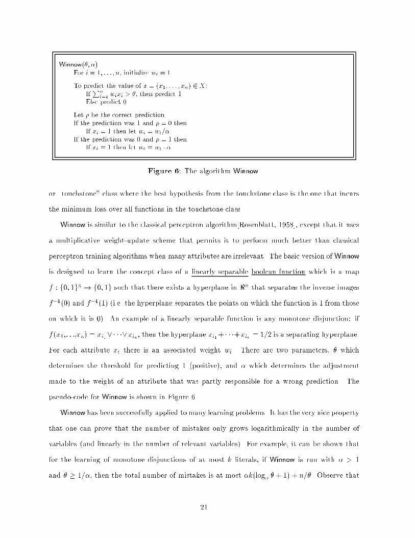
Winnow�� �For i � �� � � � � n� initialize wi � �

To predict the value of x � �x�� � � � � xn� � X�IfPn

i � wixi � � then predict �Else predict

Let � be the correct predictionIf the prediction was � and � � then

If xi � � then let wi � wi�If the prediction was and � � � then

If xi � � then let wi � wi

Figure � The algorithm Winnow�

or �touchstone� class where the best hypothesis from the touchstone class is the one that incurs

the minimum loss over all functions in the touchstone class�

Winnow is similar to the classical perceptron algorithm�Rosenblatt� �� �� except that it uses

a multiplicative weight�update scheme that permits it to perform much better than classical

perceptron training algorithms when many attributes are irrelevant� The basic version of Winnow

is designed to learn the concept class of a linearly separable boolean function which is a map

f � f�� gn � f�� g such that there exists a hyperplane in �n that separates the inverse images

f����� and f���� �i�e� the hyperplane separates the points on which the function is from those

on which it is ��� An example of a linearly separable function is any monotone disjunction� if

f�x��� � ��xn� � xi� � � � xik � then the hyperplane xi�� � � ��xik � � is a separating hyperplane�

For each attribute xi there is an associated weight wi� There are two parameters� � which

determines the threshold for predicting �positive�� and � which determines the adjustment

made to the weight of an attribute that was partly responsible for a wrong prediction� The

pseudo�code for Winnow is shown in Figure ��

Winnow has been successfully applied to many learning problems� It has the very nice property

that one can prove that the number of mistakes only grows logarithmically in the number of

variables �and linearly in the number of relevant variables�� For example� it can be shown that

for the learning of monotone disjunctions of at most k literals� if Winnow is run with � �

and � � �� then the total number of mistakes is at most �k�log � � � � n�� Observe that

�

Winnow need not have prior knowledge of k although the number of mistakes depends on k�

�Littlestone� � �� showed how to optimally choose � and � if an upperbound on k is known a

priori� Also� while Winnow is designed to learn a linearly separable class� reductions �discussed

in Section ��� can be used to apply Winnow to classes for which the positive and negative points

are not linearly separable� e�g� k�DNF�

����� The Halving Algorithm and Weighted Majority Algorithm

We now discuss some of the key techniques for designing good on�line learning algorithms for

the special case of concept learning �i�e� learning boolean�valued functions�� If one momentarily

ignores the issue of computation time� then the halving algorithm performs very well� It works

as follows� Initially all concepts in the concept class C are candidates for the target concept�

To make a prediction for instance x� the learner takes a majority vote based on all remaining

candidates �breaking a tie arbitrarily�� Then when the feedback is received� all concepts that

disagree are removed from the set of candidates� It can be shown that at each step the number

of candidates is reduced by a factor of at least �� Thus� the number of prediction mistakes made

by the halving algorithm is at most lg jCj�

Clearly the halving algorithm will perform poorly if the data is noisy� We now brie�y discuss

the weighted majority algorithm which is one of several multiplicative weight�update schemes

for generalizing the halving algorithm to tolerate noise� Also� the weighted majority algorithm

provides a simple and eective method for constructing a learning algorithm A that is provided

with a pool of �experts�� one of which is known to perform well� but A does not know which

one� Associated with each expert is a weight that gives A�s con�dence in the accuracy of that

expert� When asked to make a prediction� A predicts by combining the votes from its experts

based on their associated weights� When an expert suggests the wrong prediction� A passes that

information to the given expert and reduces its associated weight using a multiplicative weight�

updating scheme� Namely� the weight associated with each expert that mispredicts is multiplied

by some weight � � � � By selecting � � this algorithm is robust against noise in the data�

Figure � shows the weighted majority algorithm in more depth�

We now brie�y discuss some learning problems in which weighted majority is applicable�

��

Weighted Majority Algorithm �WM�Let wi be the weight associated with algorithm Ai

For � � i � nLet wi � �

To make a prediction for an instance x � X�Let A� be the set of algorithms that predicted Let A� be the set of algorithms that predicted �Let q� �

PAi�A�

wi

Let q� �P

Ai�A�wi

Predict i� q� q�If a mistake is made�

Let be the predictionFor � � i � n

If Ai�s prediction for x is Let wi � wi � �where � � � ��Inform Ai of the mistake

Figure �� The weighted majority algorithm�

Suppose one knows that the correct prediction comes from some target concept selected from a

known concept class� Then one can apply the weighted majority algorithm where each concept in

the class is one of the algorithms in the pool� For such situations� the weighted majority algorithm

is a robust generalization of the halving algorithm� �In fact� the halving algorithm corresponds

to the special case where � ��� As another example� the weighted majority algorithm can often

be applied to help in situations in which the prediction algorithm has a parameter that must be

selected and the best choice for the parameter depends on the target� In such cases one can build

the pool of algorithms by choosing various values for the parameter�

We now describe some of the results known about the performance of the weighted majority

algorithm� If the best algorithm in the pool A makes at most m mistakes� then the worst case

number of mistakes made by the weighted majority algorithm is O�log jAj�m� where the constant

hidden within the big�oh notation depends on � Speci�cally� the number of mistakes made by

the weighted majority algorithm is at most�log jAj�m log �

�

log �

���

if one algorithm in A makes at most

m mistakes�log jAj

k�m log �

�

log �

���

if there exists a set of k algorithms in A such that each algorithm

makes at most m mistakes� andlog jAj

k�m

klog �

�

log ����

if the total number of mistakes made by a set of

k algorithms in A is m�

��

When jAj is not polynomial� the weighted majority algorithm �when directly implemented��

is not computationally feasible� Recently� �Maass and Warmuth� ���� introduced what they call

the virtual weight technique to implicitly maintain the exponentially large set of weights so that

the time to compute a prediction and then update the �virtual� weights is polynomial� More

speci�cally� the basic idea is to simulate Winnow by grouping concepts that �behave alike� on

seen examples into blocks� For each block only one weight has to be computed and one constructs

the blocks so that the number of concepts combined in each block as well as the weight for the

block can be e�ciently computed� While the number of blocks increases as new counterexamples

are received� the total number of blocks is polynomial in the number of mistakes� Thus all

predictions and updates can be performed in time polynomial in the number of blocks� which

is in turn polynomial in the number of prediction mistakes of Winnow� Many variations of the

basic weighted majority algorithm have also been studied� The results of �Cesa�Bianchi� et al��

���� demonstrate how to tune as a function of an upper bound on the noise rate�

��� Query Learning Model

A very well�studied formal learning model is the membership and equivalence query model de�

veloped by Angluin �Angluin� � �� In this model �often called the exact learning model� the

learner�s goal is to learn exactly how an unknown �boolean� target function f � taken from some

known concept class C� classi�es all instances from the domain� This goal is commonly referred

to as exact identi�cation� The learner has available two types of queries to �nd out about f �

one is a membership query� in which the learner supplies an instance x from the domain

and is told f�x�� The other query provided is an equivalence query in which the learner

presents a candidate function h and either is told that h � f �in which case learning is com�

plete�� or else is given a counterexample x for which h�x� �� f�x�� There is a very close

relationship between this learning model and the on�line learning model �supplemented with

membership queries� when applied to a classi�cation problem� Using a standard transformation

�Angluin� � � Littlestone� � �� algorithms that use membership and equivalence queries can

easily be converted to on�line learning algorithms that use membership queries� Under such a

transformation the number of counterexamples provided to the learner in response to the learner�s

��

equivalence queries directly corresponds to the number of mistakes made by the on�line algorithm�

In this model a number of interesting polynomial time algorithms are known for learning

deterministic �nite automata �Angluin� � ��� Horn sentences �Angluin� Frazier� and Pitt� �����

read�once formulas �Angluin� Hellerstein� and Karpinski� ����� read�twice DNF formulas �Aizen�

stein and Pitt� ���� decision trees �Bshouty and Mansour� ����� and many others� It is easily

shown that membership queries alone are not su�cient for e�cient learning of these classes� and

Angluin has developed a technique of �approximate �ngerprints� to show that equivalence queries

alone are also not enough �Angluin� ����� �In both cases the arguments are information theo�

retic� and hold even when the computation time is unbounded�� The work of �Bshouty� Goldman�

Hancock and Matar� ���� extended Angluin�s results to establish tight bounds on how many

equivalence queries are required for a number of these classes� Maass and Tur'an studied upper

and lower bounds on the number of equivalence queries required for learning �when computation

time is unbounded�� both with and without membership queries �Maass and Tur'an� �����

It is known that any class learnable exactly from equivalence queries can be learned in the

PAC setting �Angluin� � �� At a high level the exact learning algorithm is transformed to a

PAC algorithm by having the learner use random examples to �search� for a counterexample to

the hypothesis of the exact learner� If a counterexample is found� it is given as a response to the

equivalence query� Furthermore� if a su�ciently large sample was drawn and no counterexample

was found then the hypothesis has error at most � �with probability at least � ��� The converse

does not hold �Blum� ����� That is� there are concept classes that are e�ciently PAC learnable

but cannot be e�ciently learned in the exact model�

We now describe Angluin�s algorithm for learning monotone DNF formulas �see Figure �� A

prime implicant t of a formula f is a satis�able conjunction of literals such that t implies f but no

proper subterm of t implies f � For example� f � �a c� �b !c� has prime implicants a c� b !c�

and ab� The number of prime implicants of a general DNF formula may be exponentially larger

than the number of terms in the formula� However� for monotone DNF the number of prime

implicants is no greater than the number of terms in the formula� The key to the analysis is to

show that at each iteration� the term t is a new prime implicant of f � the target concept� Since

��

Learn�Monotone�DNFh� falseDo forever

Make equivalence query with hIf �yes�� output h and haltElse let x � b�b� bn be the counterexample

Let t �Vbi � yi

For i � �� � � � � nIf bi � � perform membership query on x with ith bit �ippedIf �yes�� t � t n fyig and x � b� �bi bn

Let h � h � t

Figure �� An algorithm that uses membership and equivalence queries to exactly learn an

unknown monotone DNF formula over the domain f�� gn� Let fy�� y�� � � � � yng be the boolean

variables and let h be the learner�s hypothesis�

the loop iterates exactly once for each prime implicant there are at most m counterexamples

where m is the number of terms in the target formula� Since at most n membership queries are

performed during each iteration there are at most nm membership queries overall�

� Hardness Results

In order to understand what concept classes are learnable� it is essential to develop techniques

to prove when a learning problem is hard� Within the learning theory community� there are

two basic type of hardness results that apply to all of the models discussed here� There are

representation�dependent hardness results in which one proves that one cannot e�ciently

learn C using a hypothesis class of H� These hardness results typically rely on some complexity

theory assumption� such as RP �� NP� For example� given that RP �� NP� �Pitt and Warmuth�

���� showed that k�term�DNF is not learnable using the hypothesis class of k�term�DNF� While

such results provide some information� what one would really like to obtain is a hardness re�

sult for learning a concept class using any reasonable �i�e� polynomially evaluatable� hypothesis

class� �For example� while we have a representation�dependent hardness result for learning k�

For background on Complexity Classes see Chapter �� �NP dened and Chapter ��� Section � �RP dened

of this handbook�

��

term�DNF� there is a simple algorithm to PAC learn the class of k�term�DNF formulas using

a hypothesis class of k�CNF formulas�� Representation�independent hardness results meet

this more stringent goal� However� they depend on cryptographic �versus complexity theoretic�

assumptions� �Kearns and Valiant� � �� gave representation�independent hardness results for

learning several concept classes such as Boolean formulas� deterministic �nite automata� and

constant�depth threshold circuits �a simpli�ed form of �neural networks��� These hardness re�

sults are based on assumptions regarding the intractability of various cryptographic schemes such

as factoring Blum integers and breaking the RSA function�

�� Prediction�Preserving Reductions

Given that we have some representation�independent hardness result �assuming the security of

various cryptographic schemes� one would like a �simple� way to prove that other problems are

hard in a similar fashion as one proves a desired algorithm is intractable by reducing a known

NP�complete problem to it � Such a complexity theory for predictability has been provided

by �Pitt and Warmuth� ����� They formally de�ne a prediction preserving reduction from con�

cept class C over domain X to concept class C� over domain X � �denoted by C � C�� that

allows an e�cient learning algorithm for C� to be used to obtain any e�cient learning algo�

rithm for C� The requirements for such a prediction�preserving reduction are� �� an e�cient

instance transformation g from X to X �� and ��� the existence of an image concept� The instance

transformation g must be polynomial time computable� Hence if g�x� � x� then the size of x�

must be polynomially related to the size of x� So for x � Xn� g�x� � Xp�n where p�n� is some

polynomial function of n� It is also important that g be independent of the target function� We

now de�ne what is meant by the existence of an image concept� For every f � Cn there must exist

some f � � C�p�n such that for all x � Xn� f�x� � f ��g�x�� and the number of bits to represent f �

is polynomially related to the number of bits to represent f �

As an example� let C be the class of DNF formulas over X � f�� gn� and C� be the class

of monotone DNF formulas over X � � f�� g�n� We now show that C � C�� Let y�� � � � � yn be

See Chapter �� of this handbook for background on reducibility and completeness�

��

the variables for each concept from C� Let y��� � � � � y��n be the variables for C�� The intuition

behind the reduction is that variable yi for the DNF problem is associated with variable y�i�� for

the monotone DNF problem� And variable yi for the DNF problem is associated with variable

y�i for the monotone DNF problem� So for example x � b�b� � � �bn where each bi � f�� g and

g�x� � b��� b��b��� b�� � � �bn�� bn�� Given a target concept f � C� the image concept f � is

obtained by replacing each non�negated variable yi from f with y��i�� and each negated variable

yi from f with y��i� It is easily con�rmed that all required conditions are met�

If C � C�� what implications are there with respect to learnability Observe that if we

are given a polynomial prediction algorithm A� for C�� one can use A� to obtain a polynomial

prediction algorithm A for C as follows� If A� requests a labeled example then A can obtain a

labeled example x � X from its oracle and give g�x� to A�� Finally� when A� outputs hypothesis

h�� A can make a prediction for x � X using h�g�x��� Thus if C is known not to be learnable

then C� also is not learnable� Thus the reduction given above implies that the class of monotone

DNF formulas is just as hard to learn in the PAC model as the class of arbitrary DNF formulas�

Equivalently� if there were an e�cient PAC algorithm for the class of monotone DNF formulas�

then there would also be an e�cient PAC algorithm for arbitrary DNF formulas�

�Pitt and Warmuth� ���� gave a prediction preserving reduction from the class of boolean

formulas to class of DFAs� Thus since �Kearns and Valiant� � �� proved that boolean formula

are not predictable �under cryptographic assumptions�� it immediately follows that DFAs are not

predictable� In other words� DFAs cannot be e�ciently learned from random examples alone�

Recall that any algorithm to exactly learn using only equivalence queries can be converted into

an e�cient PAC algorithm� Thus if DFAs are not e�ciently PAC learnable �under cryptographic

assumptions�� it immediately follows that DFAs are not e�ciently learnable from only equivalence

queries �under cryptographic assumptions�� Contrasting this negative result� recall that DFAs

are exactly learnable from membership and equivalence queries �Angluin� � ��� and thus are

PAC learnable with membership queries�

Notice that for C � C �� the result that an e�cient learning algorithm for C� also provides an

e�cient algorithm for C relies heavily on the fact that membership queries are NOT allowed� The

�

problem created by membership queries �whether in the PAC or exact model� is that algorithm

A� for C� may make a membership query on an example x� � X � for which g���x�� is not in X �

For example� the reduction described earlier demonstrates that if there is an e�cient algorithm

to PAC learn monotone DNF formulas then there is an e�cient algorithm to PAC learn DNF

formulas� Notice that we already have an algorithm Learn�Monotone�DNF that exactly learns this

class with membership and equivalence queries �and thus can PAC learn the class when provided

with membership queries�� Yet� the question of whether or not there is an algorithm with access

to a membership oracle to PAC learn DNF formulas remains one of the biggest open questions

within the �eld� We now describe the problem with using the algorithm Learn�Monotone�DNF to

obtain an algorithm for general DNF formulas� Suppose that we have � boolean variables �thus

the domain is f�� g��� The algorithm Learn�Monotone�DNF could perform a membership query

on the example ����� While this example is in the domain f�� g� there is no x � f�� g� for

which g�x� � ����� Thus the provided membership oracle for the DNF problem cannot be

used to respond to the membership query posed by Learn�Monotone�DNF�

We now de�ne a more restricted type of reduction C �wmq C� that yields results even when

membership queries are allowed� For these reductions� we just add the following third condition

to the two conditions already described� for all x� � X �� if x� is not in the image of g �i�e� there

is no x � X such that g�x� � x��� then the classi�cation of x� for the image concept must always

be positive or always be negative� As an example� we show that C �wmq C� where C is the class

of DNF formulas and C� is the class of read�thrice DNF formulas �meaning that each literal can

appear at most three times�� Thus learning a read�thrice DNF formula �even with membership

queries� is as hard as learning general DNF formula �with membership queries�� Let s be the

number of literals in f � �If s is not known a priori the standard doubling technique can be

applied�� The mapping g maps from an x � f�� gn to an x� � f�� gsn� More speci�cally� g�x�

simply repeats� s times� each bit of x� To see that there is an image concept� note that we have

s variables for each concept in C� associated with each variable for a concept in C� Thus we can

rewrite f � C as a formula f � � C� in which each variable only appears once� At this point we

have shown C � C � but still need to do more to satisfy the new third condition� We want to

��

ensure that the s variables �call them ���� � � � � ��s� for f � associated with one literal �i of f all take

the same value� We do this by de�ning our �nal image concept as� f � (� � � � (n where n

is the number of variables and (i is of the form ���� � ���� � � � ���s�� � ��s� ���s � ����� This

formula evaluates to true exactly when ���� � � � � ��s have the same value� Thus an x� for which no

g�x� � x� will not satisfy some (i and thus we can respond �no� to a membership query on x��

Finally� f � is a read�thrice DNF formula� This reduction also proves that boolean formulas �wmq

read�thrice boolean formulas�

� Weak Learning and Hypothesis Boosting

As originally de�ned� the PAC model requires the learner to produce� with arbitrarily high

probability� a hypothesis that is arbitrarily close to the target concept� While for many problems

it is easy to �nd simple algorithms ��rules�of�thumb�� that are often correct� it seems much harder

to �nd a single hypothesis that is highly accurate� Informally� a weak learning algorithm is

one that outputs a hypothesis that has some advantage over random guessing� �To contrast this

sometimes a PAC learning algorithm is called a strong learning algorithm�� This motivates the

question� are there concept classes for which there is an e�cient weak learner� but there is no

e�cient PAC learner Somewhat surprisingly the answer is no �Schapire� ����� The technique

used to prove this result is to take a weak learner and transform �boost� it into a PAC learner�

The general method of converting a rough rule�of�thumb �weak learner� into a highly accurate

prediction rule �PAC learner� is referred to as hypothesis boosting���

We now formally de�ne the weak learning model �Kearns and Valiant� � �� Schapire� �����

As in the PAC model� there is the instance space X and the concept class C� Also the examples

are drawn randomly and independently according to a �xed but unknown distribution D on X �

The learner�s hypothesis h must be a polynomial time function that given an x � X returns a

prediction of f�x� for f � C� the unknown target concept� The accuracy requirements for the

��We note that one can easily boost the condence � by rst designing an algorithm A that works for say � � ���

and then running A several times taking a majority vote� For an arbitrary � � � the number of runs of A needed

are polynomial in lg ����

��

hypothesis of a weak learner are as follows� There is a polynomial function p�n� and algorithm A

such that� for all n � � f � Cn� for all distributions D� and for all � � � � � algorithm A� given

n� �� and access to labeled examples from D� outputs a hypothesis h such that� with probability

� � �� errorD�h� is at most ��� p�n��� Algorithm A should run in time polynomial in n

and ��

If C is strongly learnable� then it is weakly learnable$just �x � � � �or any constant less

than ��� The converse �weak learnability implying strong learnability� is not at all obvious� In

fact� if one restricts the distributions under which the weak learning algorithm runs then weak

learnability does not imply strong learnability� Namely� �Kearns and Valiant� � �� have shown

that under a uniform distribution� monotone boolean functions are weakly� but not strongly�

learnable� Thus it is important to take advantage of the requirement that the weak learning al�

gorithm must work for all distributions� Using this property� �Schapire� ���� proved the converse

result� if concept class C is weakly learnable� then it is strongly learnable�

Proving that weak learnability implies strong learnability has also been called the hypothesis

boosting problem� because a way must be found to boost the accuracy of slightly�better�than�half

hypotheses to be arbitrarily close to � There have been several boosting algorithms proposed

since the original work of �Schapire� ����� Figure � describes AdaBoost �Freund and Schapire�

���� that has shown promise in empirical use� The key to forcing the weak learner to output

hypotheses that can be combined to create a highly accurate hypothesis is to create dierent

distributions on which the weak learner is trained�

Freund and Schapire �Freund and Schapire� ���� have done some experiments showing that

by applying AdaBoost to some simple rules of thumb or using C��� �Quinlan� ���� as the weak

learner they can perform better than previous algorithms on some standard benchmarks� Also�

Freund and Schapire have presented a more general version for AdaBoost for the situation in

which the predictions are real�valued �versus binary�� Some of the practical advantages of Ad�

aBoost are that is is fast� simple and easy to program� requires no parameters to tune �besides

T � the number of rounds�� no prior knowledge is needed about the weak learner� it is provably

eective� and it is �exible since you can combine it with any classi�er that �nds weak hypotheses�

�

AdaBoostFor i � �� � � � �m

D��i� � ��mFor t � �� � � � � T

Call WeakLearn providing it with the distribution Dt to obtain the hypothesis htCalculate the error of ht � �t �

Xi�ht�xi�� yi

Dt�i�

If �t � ���� set T � t � and abort the loopLet �t � �t��� �t�Update distribution Dt�Let Zt be a normalization constant so Dt�� is a valid probability distributionIf ht�xi� � yi

Let Dt�� �Dt�i�Zt

�tElse

Let Dt�� �Dt�i�Zt

Output the �nal hypothesis�

hfin�x� � argmaxy�Y

Xt�ht�x� y

log�

�t

Figure � The procedure AdaBoost to boost the accuracy of a mediocre hypothesis �created

by WeakLearn to a very accurate hypothesis� The input is a sequence h�x�� y��� � � � � �xm� ym�i of

labeled examples where each label comes from the set Y � f� � � � � kg�

��

� Research Issues and Summary

In this chapter� we have described the fundamental models and techniques of computational

learning theory� There are many interesting research directions besides those discussed here�

One general direction of research is in de�ning new� more realistic models� and models that cap�

ture dierent learning scenarios� Here are a few examples� Often� as in the problem of weather

prediction� the target concept is probabilistic in nature� Thus �Kearns and Schapire� ���� in�

troduced the p�concepts model� Also there has been a lot of work in extending the VC theory

to real�valued domains �e�g� �Haussler� ������ In both the PAC and on�line models� many al�

gorithms use membership queries� While most work has assumed that the answers provided to

the membership queries are reliable� in reality a learner must be able to handle inconclusive and

noisy results from the membership queries� See �Blum� Chalasani� Goldman� and Slonim� ����

for a summary of several models introduced to address this situation� As one last example� there

has been much work recently in exploring models of a �helpful teacher�� since teaching is often

used to assist human learning �e�g� �Goldman and Mathias� ���� Angluin and Krik)is� ������

Finally� there has been work to bridge the computational learning research with the research

from other �elds such as neural networks� natural language processing� DNA analysis� inductive

logic programming� information retrieval� expert systems� and many others�

� Dening Terms

Classi�cation Noise A model of noise in which the the label may be reported incorrectly�

In the random classi�cation noise model� with probability � the label is inverted� In the

malicious classi�cation noise model� with probability � an adversary can choose the label�

In both models with probability � � the example is not corrupted� The quantity � is

referred to as the noise rate�

Concept Class A set of rules from which the target function is selected�

Counterexample A counterexample x to a hypothesis h �where the target concept is f� is

either an example for which f�x� � and h�x� � � �a positive counterexample� or for

��

which f�x� � � and h�x� � �a negative counterexample��

Equivalence Query A query to an oracle in which the learner provides a hypothesis h and is

either told that h is logically equivalent to the target or otherwise given a counterexample�

Hypothesis Boosting The process of taking a weak learner that predicts correctly just over half

of the time and transforming �boosting� it into a PAC �strong� learner whose predictions

are as accurate as desired�

Hypothesis Class The class of functions from which the learner�s hypothesis is selected�

Membership Query The learner supplies the membership oracle with an instance x from the

domain and is told the value of f�x��

Occam Algorithm An algorithm that draws a sample S and then outputs a hypothesis con�

sistent with the examples in S such that the size of the hypothesis is sublinear in S �i�e� it

performs some data compression��

On�Line Learning Model The learning session consists of a set of trials where in each trial�

the learner is given an unlabeled instance x � X � The learner uses its current hypothesis

to predict a value p�x� for the unknown �real�valued� target and is then told the correct

value for f�x�� The performance of the learner is measured in terms of the sum of the loss

over all predictions�

PAC Learning This is a batch model in which �rst there is a training phase in which the learner

sees examples drawn randomly from an unknown distribution D� and labeled according to

the unknown target concept f drawn from a known concept class C� The learner�s goal is

to output a hypothesis that has error at most � with probability at least ��� �The learner

receives � and � as inputs�� In the proper PAC learning model the learner must output

a hypothesis from C� In the non�proper PAC learning model the learner can output any

hypothesis h for which h�x� can be computed in polynomial time�

Representation�Dependent Hardness Result A hardness result in which one proves that

one cannot e�ciently learn C using a hypothesis class of H� These hardness results typically

��

rely on some complexity theory assumption such as RP �� NP�

Representation�Independent Hardness Result A hardness result in which no assumption

is made about the hypothesis class used by the learner �except the hypothesis can be

evaluated in polynomial time�� These hardness results typically rely on cryptographic

assumptions such as the di�culty of breaking RSA�

Statistical Query Model A learning model in which the learner does not have access to labeled

examples� but rather only can ask queries about statistics about the labeled examples and

receive unlabeled examples� Any statistical query algorithm can be converted to a PAC

algorithm that can handle random classi�cation noise �as well as some other types of noise��

Vapnik�Chervonenkis �VC� Dimension A �nite set S � X is shattered by C if for each of

the �jSj subsets S� � S� there is a concept f � C that contains all of S� and none of S�S�� In

other words� for any of the �jSj possible labelings of S �where each example s � S is either

positive or negative�� there is some f � C that realizes the desired labeling �see Figure ���

The Vapnik�Chervonenkis dimension of C� denoted as vcd�C�� is the smallest d for which

no set of d � examples is shattered by C� Equivalently� vcd�C� is the cardinality of the

largest �nite set of points S � X that is shattered by C�

Weak Learning Model A variant of the PAC model in which the learner is only required to

output a hypothesis that with probability � � �� has error at most ��� p�n��� I�e�� it

does noticeably better than random guessing� Recall in the standard PAC �strong learning�

model the learner must output a hypothesis with arbitrarily low error�

References

�Aizenstein and Pitt� ��� Aizenstein� H� and Pitt� L� ��� Exact learning of read�

twice DNF formulas� In Proc� ��th Annu� IEEE Sympos� Found� Comput� Sci� ����� IEEE

Computer Society Press� pp� ��*���

��

�Angluin� � �� Angluin� D� � �� Learning regular sets from queries and counterexamples�

Inform� Comput� ��� � �Nov��� �*���

�Angluin� � � Angluin� D� � � Queries and concept learning� Machine Learning �� �

�April�� ��*����

�Angluin� ���� Angluin� D� ���� Negative results for equivalence queries� Machine Learn�

ing �� �*���

�Angluin� Frazier� and Pitt� ���� Angluin� D�� Frazier� M�� and Pitt� L� ���� Learn�

ing conjunctions of Horn clauses� Machine Learning �� ��*���

�Angluin� Hellerstein� and Karpinski� ���� Angluin� D�� Hellerstein� L�� and Karpinski�

M� ���� Learning read�once formulas with queries� J� ACM � �*���

�Angluin and Krik)is� ���� Angluin� D�� Krik�is� M� ���� Teachers� learners and black

boxes� In Proc� �th Annu� Conf� on Comput� Learning Theory ������ ACM Press� New

York� NY� pp� � �*����

�Angluin and Laird� � � Angluin� D� and Laird� P� � � Learning from noisy exam�

ples� Machine Learning �� �� ���*����

�Angluin and Smith� � �� Angluin� D� and Smith� C� � �� Inductive inference� In En�

cyclopedia of Arti�cial Intelligence� pp� ���*� � J� Wiley and Sons� New York�

�Anthony and Biggs� ���� Anthony� M� and Biggs� N� ���� Computational Learning

Theory� Cambridge Tracts in Theoretical Computer Science ��� Cambridge Tracts in Theo�

retical Computer Science ����� Cambridge University Press�

�Aslam and Decatur� ���� Aslam� J� A� and Decatur� S� E� ���� Speci�cation and sim�

ulation of statistical query algorithms for e�ciency and noise tolerance� Journal of Computer

and System Sciences � To appear�

��

�Blum� ���� Blum� A� ���� Separating distribution�free and mistake�bound learning mod�

els over the Boolean domain� In Proc� of the ��st Symposium on the Foundations of Comp�

Sci� ������ IEEE Computer Society Press� Los Alamitos� CA� pp� �*� �

�Blum� Chalasani� Goldman� and Slonim� ���� Blum� A�� Chalasani� P�� Goldman� S� A��

and Slonim� D� K� ���� Learning with unreliable boundary queries� In Proc� �th Annu�

Conf� on Comput� Learning Theory ������ ACM Press� New York� NY� pp� � *���

�Blumer� Ehrenfeucht� Haussler� and Warmuth� � �� Blumer� A�� Ehrenfeucht� A�� Haus�

sler� D�� and Warmuth� M� K� � �� Occam�s razor� Inform� Proc� Lett� �� ���*� ��

�Blumer� Ehrenfeucht� Haussler� and Warmuth� � �� Blumer� A�� Ehrenfeucht� A�� Haus�

sler� D�� and Warmuth� M� K� � �� Learnability and the Vapnik�Chervonenkis di�

mension� J� ACM ��� �� ���*����

�Bshouty� Goldman� Hancock� and Matar� ���� Bshouty� N�� Goldman� S�� Hancock� T��

and Matar� S� ���� Asking questions to minimize errors� Journal of Computer and

System Sciences ��� � �April�� �� *� ��

�Bshouty and Mansour� ���� Bshouty� N� H� and Mansour� Y� ���� Simple learning

algorithms for decision trees and multivariate polynomials� In Proceedings of the ��th Annual

Symposium on Foundations of Computer Science ������ IEEE Computer Society Press� Los

Alamitos� CA� pp� ���*��

�Cesa�Bianchi� Freund� Helmbold� Haussler� Schapire� and Warmuth� ���� Cesa�Bianchi� N��

Freund� Y�� Helmbold� D� P�� Haussler� D�� Schapire� R� E�� and Warmuth� M� K�

���� How to use expert advice� In Proc� ��th Annu� ACM Sympos� Theory Comput� ������

ACM Press� New York� NY� pp� � �*��� Expanded version in Univ� of Calif� Computer

Research Lab TR UCSC�CRL������� From Santa Cruz� CA�

�Devroye� Gy�or�� and Lugosi� ���� Devroye� L�� Gy�orfi� L�� and Lugosi� G� ���� A

Probabalistic Theory of Pattern Recognition� Applications of Mathematics� Applications of

Mathematics� Springer�Verlag� New York�

��

�Duda and Hart� ���� Duda� R� O� and Hart� P� E� ���� Pattern Classi�cation and

Scene Analysis� Wiley�

�Ehrenfeucht and Haussler� � �� Ehrenfeucht� A� and Haussler� D� � �� A general

lower bound on the number of examples needed for learning� Inform� Comput� ��� � �Sept���

���*���

�Freund and Schapire� ���� Freund� Y� and Schapire� R� ���� Experiments with a new

boosting algorithm� In Proceedings of the Thirteenth International Conference on Machine

Learning ������ Morgan Kaufmann� pp� � *���

�Gold� ���� Gold� E� M� ���� Language identi�cation in the limit� Inform� Control ��

���*����

�Goldman and Mathias� ���� Goldman� S� and Mathias� D� ���� Teaching a smarter

learner� J� of Comput� Syst� Sci� ��� � �April�� ���*����

�Goldman and Sloan� ���� Goldman� S� and Sloan� R� ���� Can PAC learning algo�

rithms tolerate random attribute noise Algorithmica �� �July�� ��* ��

�Goldman and Scott� ���� Goldman� S� A� and Scott� S� D� ���� A theoretical and

empirical study of a noise�tolerant algorithm to learn geometric patterns� In Proceedings of

the Thirteenth International Conference on Machine Learning ������ Morgan Kaufmann� pp�

�*���

�Haussler� ���� Haussler� D� ���� Decision theoretic generalizations of the PAC model

for neural net and other learning applications� Inform� Comput� �� �Sept��� � *���

�Haussler� Kearns� Littlestone� and Warmuth� ��� Haussler� D�� Kearns� M�� Little�

stone� N�� and Warmuth� M� K� ��� Equivalence of models for polynomial learn�

ability� Inform� Comput� ��� � �Dec��� ��*��

�Haussler� Littlestone� and Warmuth� ���� Haussler� D�� Littlestone� N�� and War�

muth� M� K� ���� Predicting f�� g functions on randomly drawn points� Inform�

Comput� ���� �� � �*����

�

�Kearns� ���� Kearns� M� ���� E�cient noise�tolerant learning from statistical queries�

In Proc� ��th Annu� ACM Sympos� Theory Comput� ������ ACM Press� New York� NY� pp�

���*���

�Kearns and Valiant� � �� Kearns� M� and Valiant� L� G� � �� Cryptographic limita�

tions on learning Boolean formulae and �nite automata� In Proc� of the ��st Symposium on

Theory of Computing �� ��� ACM Press� New York� NY� pp� ���*����

�Kearns and Vazirani� ���� Kearns� M� and Vazirani� U� ���� An Introduction to Com�

putational Learning Theory� MIT Press� Cambridge� Massachusetts�

�Kearns and Schapire� ���� Kearns� M� J� and Schapire� R� E� ���� E�cient

distribution�free learning of probabilistic concepts� In Proc� of the ��st Symposium on the

Foundations of Comp� Sci� ������ IEEE Computer Society Press� Los Alamitos� CA� pp�

� �*���

�Kearns� Schapire� and Sellie� ���� Kearns� M� J�� Schapire� R� E�� and Sellie� L� M�

���� Toward e�cient agnostic learning� Machine Learning ��� ���� �*���

�Kodrato and Michalski� ���� Kodratoff� Y� and Michalski� R� S�� Eds� ���� Ma�

chine Learning� An Arti�cial Intelligence Approach� vol� III� Morgan Kaufmann� Los Altos�

California�

�Littlestone� � � Littlestone� N� � � Learning when irrelevant attributes abound� A

new linear�threshold algorithm� Machine Learning �� � �*� �

�Maass and Tur'an� ���� Maass� W� and Tur�an� G� ���� Lower bound methods and

separation results for on�line learning models� Machine Learning �� ��*���

�Maass and Warmuth� ���� Maass� W� and Warmuth� M� K� ���� E�cient learning

with virtual threshold gates� In Proc� ��th International Conference on Machine Learning

������ Morgan Kaufmann� pp� �� *� ��

�Natarajan� ��� Natarajan� B� K� ��� Machine Learning� A Theoretical Approach�

Morgan Kaufmann� San Mateo� CA�

��

�Pitt and Valiant� � � Pitt� L� and Valiant� L� � � Computational limitations on

learning from examples� J� ACM ��� ���*� ��

�Pitt and Warmuth� ���� Pitt� L� and Warmuth� M� K� ���� Prediction preserving

reducibility� J� of Comput� Syst� Sci� �� � �Dec��� ���*���� Special issue of the for the Third

Annual Conference of Structure in Complexity Theory �Washington� DC�� June ��

�Quinlan� ���� Quinlan� J� R� ���� C��� Programs for machine learning� Morgan Kauf�

mann�

�Rosenblatt� �� � Rosenblatt� F� �� � The perceptron� A probabilistic model for in�

formation storage and organization in the brain� Psych� Rev� ��� � �*���� �Reprinted in

Neurocomputing �MIT Press� � ����

�Schapire� ���� Schapire� R� E� ���� The strength of weak learnability� Machine Learn�

ing �� �� ��*����

�Sloan� � � Sloan� R� � � Types of noise in data for concept learning� In Proc� �st

Annu� Workshop on Comput� Learning Theory �San Mateo� CA� � �� Morgan Kaufmann�

pp� �*���

�Valiant� � �� Valiant� L� G� � �� A theory of the learnable� Commun� ACM ���

�Nov��� ��*���

�Valiant� � �� Valiant� L� G� � �� Learning disjunctions of conjunctions� In Proceed�

ings of the �th International Joint Conference on Arti�cial Intelligence� vol� � �Los Angeles�

California� � ��� International Joint Committee for Arti�cial Intelligence� pp� ���*����

�Vapnik and Chervonenkis� ��� Vapnik� V� N� and Chervonenkis� A� Y� ��� On the

uniform convergence of relative frequencies of events to their probabilities� Theory of Probab�

and its Applications ��� �� ���*� ��

��

Further Information

Good introductions to computational learning theory �along with pointers to relevant liter�

ature� can be found in such textbooks as �Kearns and Vazirani� ������Natarajan� ���� and

�Anthony and Biggs� ����� Many recent results can be found in the proceedings from the fol�

lowing conferences� ACM Conference on Computational Learning Theory �COLT�� European

Conference on Computational Learning Theory �EuroCOLT�� International Workshop on Algo�

rithmic Learning Theory �ALT�� International Conference on Machine Learning �ICML�� IEEE

Symposium on Foundations of Computer Science �FOCS�� ACM Symposium on Theoretical

Computing �STOC�� and Neural Information Processing Conference �NIPS��

Some major journals in which many learning theory papers can be found are� Machine

Learning� Journal of the ACM� SIAM Journal of Computing� Information and Computation� and

Journal of Computer and System Sciences� See �Kodrato and Michalski� ���� for background

information on machine learning� and see �Angluin and Smith� � �� for a discussion of inductive

inference models and research�

�