ROYAL HOLLOWAY UNIVERISTY OF LONDON

JPEG compression How images are generally compressed using JPEG

Candidate Number: 1600085

Contents Compression using JPEG ..................................................................................................................................................... 1

YCbCr colour transform ........................................................................................................................................................ 1

Down Sampling ................................................................................................................................................................... 2

Discrete Cosine Transform (DCT): ....................................................................................................................................... 2

Discrete Cosine Transform formulae: ............................................................................................................................. 4

Quantization: ...................................................................................................................................................................... 5

Entropy Coding:................................................................................................................................................................... 6

Conclusion ........................................................................................................................................................................... 8

Questions not answered in this Project: ............................................................................................................................. 8

Bibliography: ....................................................................................................................................................................... 9

1 Candidate number: 1600085

Compression using JPEG JPEG is a widely known compression method used to store images efficiently. JPEG reduces the size of the original image

at the cost of image quality. The size is greatly reduced and the change in quality is almost undetectable by human eye.

The quality of image is reduced because some data is discarded and is unrecoverable which classes JPEG as a lossy

compression method. This is of course different from the lossless data compression methods such as PNG in which there

is no loss of image data. By using JPEG, images can be reduced to roughly 5% of the normal size which saves tremendous

amount of storage and is particularly useful for companies that store huge amounts of images.

JPEG Compression procedure:

Original image

in RGB

YCbCr colour transform

Down

Sampling

Discrete Cosine

Transform

Quantization

Entropy

Encoding

Encoded JPEG

image

Original Image in RGB colour space

Images are made up of pixels and the colour of each pixel in the original image can be represented by 3-dimensional

vector (R,G,B). The colour of each pixel can be specified using intensities of red, green and blue. The intensity of each

colour varies from 0 to 255. Hence each color component can be represented as an integer. In a typical natural image,

there is a significant amount of correlation between these components i.e. take a pixel and the pixels around this pixel

will be similar. It is consequence of the fast that surfaces are smooth. Our aim is to find redundancies in order to reduce

the amount of data required to represent the image.

YCbCr colour transform We use colour space transform from RGB to YCbCr whose vector components represent luminance (Y), blue chrominance

(Cb) and red chrominance (Cr). Note that YCbCr is not a colour space but rather a way of encoding RGB information.

Below is the transformation matrix which converts RGB to YCbCr. The matrix is constant and most importantly invertible

meaning that we can transform back to RGB when reconstructing the image.

We split the image into blocks (Figure 1) where each block consists of 8x8 pixels, one of the blocks from figure 1 is

zoomed in to show 8x8 pixel block in Figure 2. If the image cannot be divided exactly into 8x8 pixel blocks then we add

extra information.

Figure 1 Figure 2

2 Candidate number: 1600085

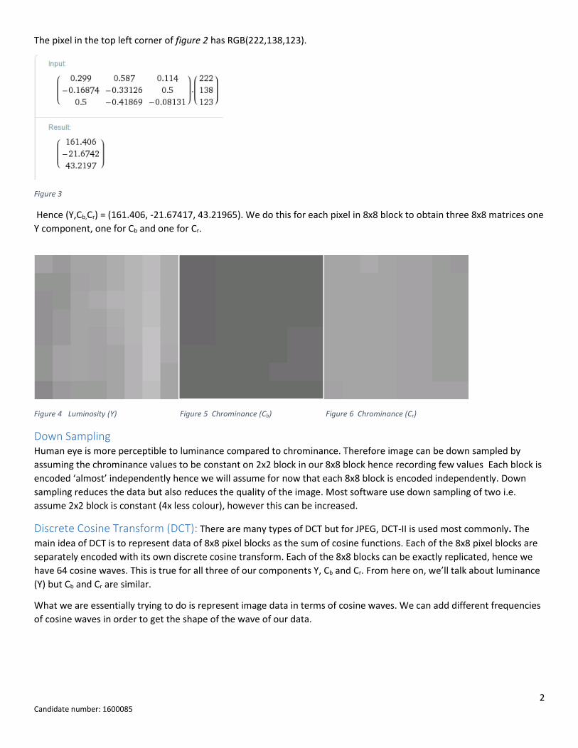
The pixel in the top left corner of figure 2 has RGB(222,138,123).

Figure 3

Hence (Y,Cb,Cr) = (161.406, -21.67417, 43.21965). We do this for each pixel in 8x8 block to obtain three 8x8 matrices one

Y component, one for Cb and one for Cr.

Figure 4 Luminosity (Y) Figure 5 Chrominance (Cb) Figure 6 Chrominance (Cr)

Down Sampling Human eye is more perceptible to luminance compared to chrominance. Therefore image can be down sampled by

assuming the chrominance values to be constant on 2x2 block in our 8x8 block hence recording few values Each block is

encoded ‘almost’ independently hence we will assume for now that each 8x8 block is encoded independently. Down

sampling reduces the data but also reduces the quality of the image. Most software use down sampling of two i.e.

assume 2x2 block is constant (4x less colour), however this can be increased.

Discrete Cosine Transform (DCT): There are many types of DCT but for JPEG, DCT-II is used most commonly. The

main idea of DCT is to represent data of 8x8 pixel blocks as the sum of cosine functions. Each of the 8x8 pixel blocks are

separately encoded with its own discrete cosine transform. Each of the 8x8 blocks can be exactly replicated, hence we

have 64 cosine waves. This is true for all three of our components Y, Cb and Cr. From here on, we’ll talk about luminance

(Y) but Cb and Cr are similar.

What we are essentially trying to do is represent image data in terms of cosine waves. We can add different frequencies

of cosine waves in order to get the shape of the wave of our data.

3 Candidate number: 1600085

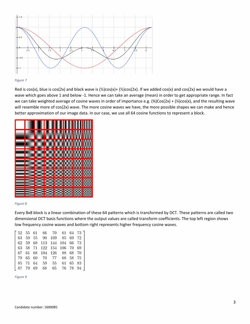
Figure 7

Red is cos(x), blue is cos(2x) and black wave is (½)cos(x)+ (½)cos(2x). If we added cos(x) and cos(2x) we would have a

wave which goes above 1 and below -1. Hence we can take an average (mean) in order to get appropriate range. In fact

we can take weighted average of cosine waves in order of importance e.g. (¾)Cos(2x) + (¼)cos(x), and the resulting wave

will resemble more of cos(2x) wave. The more cosine waves we have, the more possible shapes we can make and hence

better approximation of our image data. In our case, we use all 64 cosine functions to represent a block.

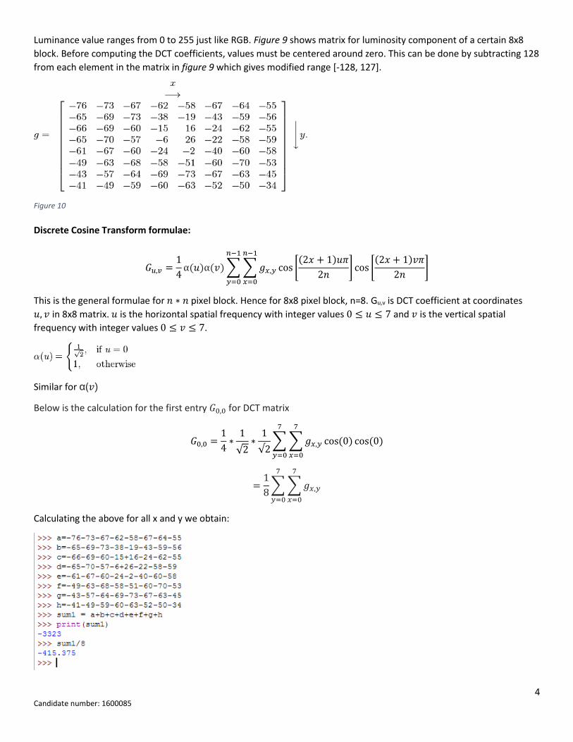
Figure 8

Every 8x8 block is a linear combination of these 64 patterns which is transformed by DCT. These patterns are called two

dimensional DCT basis functions where the output values are called transform coefficients. The top left region shows

low frequency cosine waves and bottom right represents higher frequency cosine waves.

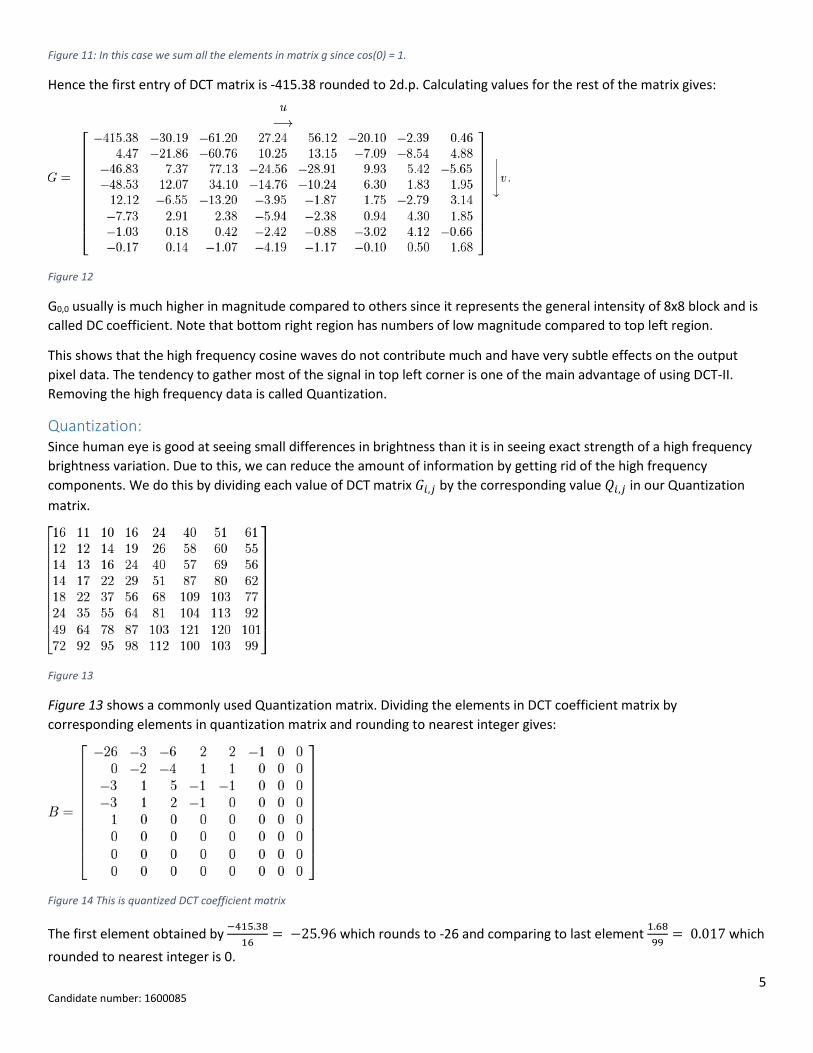
Figure 9

4 Candidate number: 1600085

Luminance value ranges from 0 to 255 just like RGB. Figure 9 shows matrix for luminosity component of a certain 8x8

block. Before computing the DCT coefficients, values must be centered around zero. This can be done by subtracting 128

from each element in the matrix in figure 9 which gives modified range [-128, 127].

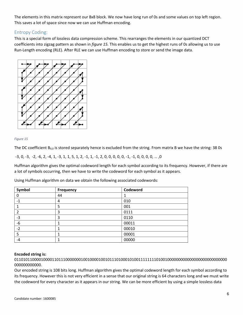
Figure 10

Discrete Cosine Transform formulae:

𝐺𝑢,𝑣 =1

4α(𝑢)α(𝑣) ∑ ∑ 𝑔𝑥,𝑦 cos [

(2𝑥 + 1)𝑢𝜋

2𝑛]

𝑛−1

𝑥=0

𝑛−1

𝑦=0

cos [(2𝑥 + 1)𝑣𝜋

2𝑛]

This is the general formulae for 𝑛 ∗ 𝑛 pixel block. Hence for 8x8 pixel block, n=8. Gu,v is DCT coefficient at coordinates

𝑢, 𝑣 in 8x8 matrix. 𝑢 is the horizontal spatial frequency with integer values 0 ≤ 𝑢 ≤ 7 and 𝑣 is the vertical spatial

frequency with integer values 0 ≤ 𝑣 ≤ 7.

Similar for α(𝑣)

Below is the calculation for the first entry 𝐺0,0 for DCT matrix

𝐺0,0 =1

4∗

1

√2∗

1

√2∑ ∑ 𝑔𝑥,𝑦 cos(0)

7

𝑥=0

7

𝑦=0

cos(0)

=1

8∑ ∑ 𝑔𝑥,𝑦

7

𝑥=0

7

𝑦=0

Calculating the above for all x and y we obtain:

5 Candidate number: 1600085

Figure 11: In this case we sum all the elements in matrix g since cos(0) = 1.

Hence the first entry of DCT matrix is -415.38 rounded to 2d.p. Calculating values for the rest of the matrix gives:

Figure 12

G0,0 usually is much higher in magnitude compared to others since it represents the general intensity of 8x8 block and is

called DC coefficient. Note that bottom right region has numbers of low magnitude compared to top left region.

This shows that the high frequency cosine waves do not contribute much and have very subtle effects on the output

pixel data. The tendency to gather most of the signal in top left corner is one of the main advantage of using DCT-II.

Removing the high frequency data is called Quantization.

Quantization: Since human eye is good at seeing small differences in brightness than it is in seeing exact strength of a high frequency

brightness variation. Due to this, we can reduce the amount of information by getting rid of the high frequency

components. We do this by dividing each value of DCT matrix 𝐺𝑖,𝑗 by the corresponding value 𝑄𝑖,𝑗 in our Quantization

matrix.

Figure 13

Figure 13 shows a commonly used Quantization matrix. Dividing the elements in DCT coefficient matrix by

corresponding elements in quantization matrix and rounding to nearest integer gives:

Figure 14 This is quantized DCT coefficient matrix

The first element obtained by −415.38

16= −25.96 which rounds to -26 and comparing to last element

1.68

99= 0.017 which

rounded to nearest integer is 0.

6 Candidate number: 1600085

The elements in this matrix represent our 8x8 block. We now have long run of 0s and some values on top left region.

This saves a lot of space since now we can use Huffman encoding.

Entropy Coding: This is a special form of lossless data compression scheme. This rearranges the elements in our quantized DCT

coefficients into zigzag pattern as shown in figure 15. This enables us to get the highest runs of 0s allowing us to use

Run-Length encoding (RLE). After RLE we can use Huffman encoding to store or send the image data.

Figure 15

The DC coefficient B0,0 is stored separately hence is excluded from the string. From matrix B we have the string: 38 0s

-3, 0, -3, -2, -6, 2, -4, 1, -3, 1, 1, 5, 1, 2, -1, 1, -1, 2, 0, 0, 0, 0, 0, -1, -1, 0, 0, 0, 0, … ,0

Huffman algorithm gives the optimal codeword length for each symbol according to its frequency. However, if there are

a lot of symbols occurring, then we have to write the codeword for each symbol as it appears.

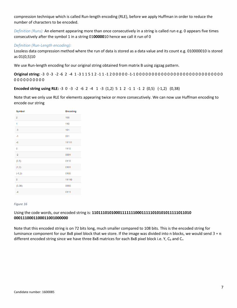
Using Huffman algorithm on data we obtain the following associated codewords:

Symbol Frequency Codeword

0 44 1

-1 4 010

1 5 001

2 3 0111

-3 3 0110

-6 1 00011

-2 1 00010

5 1 00001

-4 1 00000

Encoded string is: 011010110000100001101110000000100100001001011101000101001111111101001000000000000000000000000000000000000000. Our encoded string is 108 bits long. Huffman algorithm gives the optimal codeword length for each symbol according to

its frequency. However this is not very efficient in a sense that our original string is 64 characters long and we must write

the codeword for every character as it appears in our string. We can be more efficient by using a simple lossless data

7 Candidate number: 1600085

compression technique which is called Run-length encoding (RLE), before we apply Huffman in order to reduce the

number of characters to be encoded.

Definition (Runs): An element appearing more than once consecutively in a string is called run e.g. 0 appears five times

consecutively after the symbol 1 in a string 010000010 hence we call it run of 0

Definition (Run-Length encoding):

Lossless data compression method where the run of data is stored as a data value and its count e.g. 010000010 is stored

as 01(0,5)10

We use Run-length encoding for our original string obtained from matrix B using zigzag pattern.

Original string: -3 0 -3 -2 -6 2 -4 1 -3 1 1 5 1 2 -1 1 -1 2 0 0 0 0 0 -1-1 0 0 0 0 0 0 0 0 0 0 0 0 0 0 0 0 0 0 0 0 0 0 0 0 0 0 0 0

0 0 0 0 0 0 0 0 0 0

Encoded string using RLE: -3 0 -3 -2 -6 2 -4 1 -3 (1,2) 5 1 2 -1 1 -1 2 (0,5) (-1,2) (0,38)

Note that we only use RLE for elements appearing twice or more consecutively. We can now use Huffman encoding to

encode our string

Figure 16

Using the code words, our encoded string is: 1101110101000111111100011111010101011111011010 0001110001100011001000000 Note that this encoded string is on 72 bits long, much smaller compared to 108 bits. This is the encoded string for luminance component for our 8x8 pixel block that we store. If the image was divided into n blocks, we would send 3 ∗ 𝑛 different encoded string since we have three 8x8 matrices for each 8x8 pixel block i.e. Y, Cb and Cr.

8 Candidate number: 1600085

Conclusion This completes the general procedure for JPEG compression. Different software may use different variations in each stage e.g. higher ratio of down sampling of chrominance, different quantization matrix or different lossless encoding method for entropy encoding and other minor changes to achieve the required size or quality. However the general idea remains the same. Each of the stages are obviously reversible in order to reconstruct the original image. Some data is lost permanently and quality of the image may be lowered. Although in most cases, human eye would not be able to distinguish the difference between JPEG and the original image.

Questions not answered in this Project: 1. How 3x3 matrix for RGB to YCbCr derived and why are there different variations of these matrices?

2. How is the quantization matrix derived? What is the optimal Quantizer?

3. How is DCT formulae derived?

4. There are many other types of transforms such as Kahunen-Loeve transform, Discrete Fourier transform etc.

Why use DCT-II?

Karhunen–Loève transform (KLT) minimizes the total mean square error for the pixels. In fact it gives optimal

error however KLT is not used in practice since the co-efficient matrix is not constant and is image dependent.

This costs too much and is computationally slow. In fact for certain types of images, DCT is Kahunen-Loeve

transform. Also DCT assumes the pixels next to each other are similar, which is a reasonable assumption since

natural images are smooth and pixels are highly correlated. Discrete Cosine Transform is suboptimal but it is

very fast and efficient. However, more research is needed to answer this question in more depth.

9 Candidate number: 1600085

Bibliography:

[1] David Austin, Image Compression: Seeing What’s Not There [online]. Grand Valley State Univeristy [viewed 08 Jan 2016] Available from: http://www.ams.org/samplings/feature-column/fcarc-image-compression [2] Randell Heyman, How JPEG works. 23 Jan 2015 [viewed 02 Jan 2016] Available from: https://www.youtube.com/watch?v=f2odrCGjOFY [3] Mikulic, Discrete Cosine Transform. 01 Sept 2001 [viewed 04 Jan 2016] Available from: https://unix4lyfe.org/dct/ [4] JPEG: Wikipedia. 08 Jan 2016 [viewed 06 Jan 2016] Available from: https://en.wikipedia.org/wiki/JPEG#Discrete_cosine_transform [5] Discrete Cosine Transform: Wikipedia. 20 Dec 2015 [viewed 04 Jan 2016] Available from: https://en.wikipedia.org/wiki/Discrete_cosine_transform [6] Dheera Venkatraman, Online Plotting tool. Available from: http://fooplot.com/#W3sidHlwZSI6MTAwMH1d [7] Timur, Huffman coding calculator. Available from: http://planetcalc.com/2481/ [8] JPEG ‘files’ & Colour (JPEG Pt1): Computerphile. 21 Apr 2015 [viewed 28 dec 2015]. Available from: https://www.youtube.com/watch?v=n_uNPbdenRs [9] JPEGDCT, Discrete Cosine Transform (JPEG Pt2): Computerphile. 22 May 2015 [viewed 28 dec 2015]. Available from: https://www.youtube.com/watch?v=Q2aEzeMDHMA [10] Digital image processing: p010 – The Discrete Cosine Transform (DCT): Alireza Saberi. 15 March 2013 [viewed 02 Jan 2016]. Available from: https://www.youtube.com/watch?v=_bltj_7Ne2c [11] Digital image processing: p009 JPEGs 8x8 blocks: Alireza Saberi. 15 March 2013 [viewed 02 Jan 2016]. Available from: https://www.youtube.com/watch?v=pZuaOjfsv0Y [12] Run-length encoding: Wikipedia. 07 Dec 2015 [viewed 08 Jan 2016]. Available from: https://en.wikipedia.org/wiki/Run-length_encoding