NBER WORKING PAPER SERIES

COMPREHENSIVE VERSUS SELECTIVE SCHOOLING IN ENGLAND IN WALES:

WHAT DO WE KNOW?

Jörn-Steffen PischkeAlan Manning

Working Paper 12176http://www.nber.org/papers/w12176

NATIONAL BUREAU OF ECONOMIC RESEARCH1050 Massachusetts Avenue

Cambridge, MA 02138April 2006

We thank Ghazala Azmat and Michele Pellizzari for excellent research assistance. We thank seminarparticipants at the NBER Education Program Meetings and particularly Esther Duflo for helpful commentson a previous version of this paper. Pischke thanks the NBER for their hospitality during a visit when muchof the work for this project was performed. The views expressed herein are those of the author(s) and do notnecessarily reflect the views of the National Bureau of Economic Research.

©2006 by Jörn-Steffen Pischke and Alan Manning. All rights reserved. Short sections of text, not to exceedtwo paragraphs, may be quoted without explicit permission provided that full credit, including © notice, isgiven to the source.

Comprehensive versus Selective Schooling in England in Wales: What Do We Know?Jörn-Steffen Pischke and Alan Manning NBER Working Paper No. 12176April 2006JEL No. I21, I28

ABSTRACT

British secondary schools moved from a system of extensive and early selection and tracking in

secondary schools to one with comprehensive schools during the 1960s and 70s. Before the reform,

students would take an exam at age eleven, which determined whether they would attend an

academically oriented grammar school or a lower level secondary school. The reform proceeded at

an uneven pace in different areas, so that both secondary school systems coexist during the 1960s

and 70s. The British transition therefore provides an excellent laboratory for the study of the impact

of a comprehensive versus a selective school system on student achievement. Previous studies

analyzing this transition have typically used a value-added methodology: they compare outcomes

for students passing through either type of school controlling for achievement levels at the time of

entering secondary education. While this seems like a reasonable research design, we demonstrate

that it is unlikely to successfully eliminate selection effects in who attends what type of school. Very

similar results are obtained by looking at the effect of secondary school environment on achievement

at age 11 and controlling for age 7 achievement. Since children only enter secondary school at age

11, these effects are likely due to selection bias. Careful choice of treatment and control areas, and

using political control of the county as an instrument for early implementation of the comprehensive

regime do not solve this problem.

Jörn-Steffen Pischke Centre for Economic Performance London School of Economics Houghton Street London WC2A 2AE UKand NBERs.pischke@lse.ac.uk

Alan ManningCentre for Economic Performance London School of Economics Houghton Street London WC2A 2AE UKa.manning@lse.ac.uk

1

Introduction

National school systems differ widely in the amount of ability tracking of students they provide

in secondary school. Some systems (e.g. the US) are based on comprehensive schools, where

students of all abilities attend the same school, although there is typically some tracking within

schools. Other systems (e.g. Germany) channel students at an early age into different types of

schools based on academic ability. British schools moved from a system of extensive tracking to

one with comprehensive schools in the 1960s and 70s. The British experience is interesting,

because it involved a major and well defined change in terms of the ability grouping of

secondary school students. Hence, it offers potentially very promising research designs in order

to assess the impact of the secondary school regime on student achievement. It is unsurprising

that numerous studies in the education and economics of education literatures analyze the British

experience.

In the traditional British school system, students were tracked into either an academically

selective grammar school at age 11, or they would attend a secondary modern school, which was

academically less demanding. Starting in the 1950s, there was dissatisfaction with selection at

the local level, and some local authorities began to experiment with comprehensive schools. In

1965, the central government asked the Local Education Authorities (LEAs) to draw up plans to

switch to a comprehensive system. The implementation proceeded slowly, with faster growing,

more Labour leaning LEAs moving to comprehensive schools more quickly, while those without

expanding numbers of students, and more Conservative leaning Authorities implemented the

change more slowly. In fact, there are still a number of LEAs to date which provide grammar

schools as an option.

Much of the research on comprehensive education in Britain uses the National Child

Development Study (NCDS), a panel which tracks members of the 1958 birth cohort. The

sample members entered secondary school in 1969, at a time when some LEAs in Britain had

started to provide comprehensive schools already, while others continued to offer the traditional

selective schools. Hence, the comparisons using the NCDS are essentially cross-sectional.

While Kerckhoff et al. (1996) claim that comprehensive areas differ little from selective areas,

we find that comprehensive areas are systematically poorer, and have students with lower

previous achievement. A raw comparison of students attending comprehensive and selective

2

schools is therefore not possible. Most previous studies rely on some form of a value added

specification, where student performance at age 16 is a function of student performance at age

11, the secondary school environment, and possibly other control variables.

This seems an entirely reasonably research design, particularly since the NCDS offers a large set

of controls on student ability and family background. We demonstrate in this paper that this

methodology is nevertheless unlikely to be completely successful in removing the selection bias

between comprehensive and selective school students. The NCDS provides test scores at ages 7,

11, and 16. It is therefore possible to run an analogous specification for student performance at

age 11 on student performance at age 7, and the secondary school environment. Since students

at age 11 have not started attending secondary school yet, the secondary school environment

should have no influence on age 11 outcomes if the specification successfully removes the

selection bias. This exercise is therefore a falsification test for the value added specification.

OLS value added specifications tend to lead to a small negative average effect of comprehensive

schooling compared to selective schooling in our sample. We demonstrate that effects of a

similar size or larger are obtained when using age 11 test scores as outcomes. This suggests that

the methodology is unable to remove the selection bias between students attending different

schools. A more interesting finding of the previous literature (particularly Kerkhoff et al., 1996)

may be that comprehensive schools tend to be equalizing, in that they lower the performance of

the most able students, and raise the performance of the least able. We show that this result is

also likely due to selection bias.

We also demonstrate that various approaches to improve on the methodology used previously are

not more successful. Most studies on this question compare students attending comprehensive

and selective schools. Since many LEAs were in the middle of comprehensive reorganization in

the 1970s, these schools often coexisted within the same LEA. A better use of the policy

variation, possibly removing some of the selection, is the comparison of LEAs which are either

purely comprehensive or purely selective in 1969, when the NCDS cohort enters secondary

school. We show that this does not help in removing the selection bias. Another approach is the

use of instrumental variables (IV) for comprehensive reorganization (see, for example, Galinda-

Rueda and Vignoles, 2004). Political control of the county is a good predictor of early

3

reorganization, and conditional on county socio demographic characteristics is a plausible

instrument. We show that the IV strategy similarly fails.

At a theoretical level, there are good arguments for selection as well as for comprehensive

education. The main argument for selection or tracking is presumably that it is much easier to

teach lower variance classes. Since teachers can focus on the ability level of particular groups of

students, students of all ability levels might benefit from selection. One argument against

selection is that there might be positive peer effects from the most able students. By tracking

these students into separate classrooms, the most able students may benefit from being with each

other. However, the lower ability ranges loose from not having this peer group around. We

know very little about the different impact of peer group effects on different types of students

empirically, so it is difficult to judge a priori whether this leads to lower or higher average

performance in a selective system.

Another argument, particularly against early selection as in post-war Britain, is that eventual

ability levels are difficult to predict at an age as early as 10 or 11. Moreover, secondary selection

is based on a single exam, clearly a noisy mechanism. This may result in some kids ending up in

the wrong track. This suggests that particularly middle ability kids may loose in the British style

selective system. Since there are arguments going either way, the issue eventually is an

empirical one.

The findings in the empirical literature about selection differ widely. Many researchers looking

at the British secondary reorganization conclude that the evidence does not support claims to the

superiority of either system (see, for example, Crook, Power, and Whitty, 1999). On the other

hand, there are also studies which find more pronounced effects going one way or the other.

Jesson (2000) uses data from the 1990s on those LEAs which still remain selective. Also using a

value added approach, he argues that comprehensive LEAs systematically outperform selective

LEAs in Britain. Based on the findings from the NCDS, these results are equally suspect. We

conclude that little can be learned from the existing literature on the British reorganization on the

performance of comprehensive versus selective schools.

Two recent papers by Hansushek and Wößmann (2006) and Waldinger (2006) apply an approach

roughly similar to ours to educational inequality across countries. Both papers investigate

4

whether inequality in educational outcomes is related to the amount of secondary school tracking

and selection across countries. These papers apply a differences-in-differences approach

comparing outcomes between secondary and primary schooling. Hanushek and Wößmann find

evidence that tracking raises educational inequality, while Waldinger does not. However,

Waldinger shows that the Hanushek and Wößmann results are not very robust to alternative

sample and variable specifications.

The remainder of this paper is organized as follows. The next section briefly describes the

institutional background of British secondary education, and the history of comprehensive

reorganization. Section 3 discusses the empirical framework, and the approaches used in some

of the existing literature. The following section describes the data and key variables. Results are

discussed in section 5, and the final section concludes.

Secondary Education in Britain1

After World War II, secondary education was provided mainly in grammar and secondary

modern schools. The 11+ exam, taken at the age of 10 or 11, determined whether a student was

allowed to attend the selective and academically oriented grammar school. About 25 percent of

students would attend grammars, with the remainder attending less challenging secondary

modern schools. While this was the consensus model, education policy making in Britain was

always rather decentralized, with the local educational authorities (LEAs) being the main

administrative units, which retained a lot of decision making power about the exact make-up of

the local school system. The 1944 Education Act only prescribed separate secondary schools

and a transfer at age 11 leaving open the possibility for LEAs to experiment with other schemes,

including comprehensive schools. Early drives for the establishment of comprehensives at the

local level were typically, although not exclusively, in Labour dominated urban areas, like

London, Bristol, and Coventry.

The existing consensus about secondary schooling at the national level also began to crack in the

1950s. There was growing unease about the selection process using the 11+ examination, which

1 This section draws heavily on the descriptions in Kerkhoff et al. (1996) and Griffith (1971).

5

determined the admission to grammar schools. Moreover, it became obvious that there were

other alternatives to a selective system than large comprehensive schools serving all children age

11 to 18 at once. The Leicestershire LEA, for example, began to experiment with abandoning

the 11+ and creating a comprehensive school up to age 14.

By the early 1960s, many, if not most, LEAs were working on reorganization plans, which were

trying to end the traditional selective system, or were challenging it in one way or another.

While Labour led LEAs played a leading role in this development, the trend cut across party

lines, with some Conservative authorities being among the most fervent advocates to ending

selection. As a response, the 1964 Education Act passed by the Conservative government

abandoned the principle of school transfer at age 11.

Only in 1963 had the Labour Party fully embraced the comprehensive principle at the national

level and called for the end of selection at their party conference. When Labour came to power

in 1964, its goal was to accelerate the existing trend for comprehensive reorganization, which

was well underway at the local level. However, there was a great diversity of views on how this

reorganization should be achieved. Rather than compelling LEAs on a particular system of

comprehensive schooling, the government issued Circular 10/65 in July 1965, requesting local

authorities to submit detailed plans on how to establish comprehensives. The circular itself

suggested no fewer than six different models of comprehensive reorganization. The middle

school model, pioneered in Leicestershire, often turned out to be popular with Conservatives,

because it allowed them to retain the grammar schools as the upper schools (an example is the

Leeds LEA). Nevertheless, in practice, most comprehensive schools eventually became 11 – 16

or 11 – 18 schools.

By the mid-1960s, secondary education in England and Wales was rather diverse. In some

LEAs, comprehensive reorganization had been well under way for years. The majority were

drawing up plans to respond to the central government’s request in some way or another. A

small number of LEAs resisted the call by the central government completely. This diversity

was not limited to the LEAs but often extended to divisions and districts within the LEAs.

Overall, the period from 1965 to 1974 was one where new comprehensive schools were

established in most parts of the country, and the fraction of students served by these schools

increased dramatically. In 1965, there were still only 262 comprehensive schools in England and

6

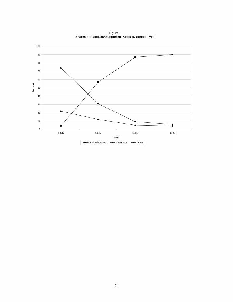
Wales. By 1974 this number had grown to 2,677, and these were attended by 62 percent of

secondary students in LEA maintained schools (see Figure 1).

One of the key issues of contention during this period was less the establishment of

comprehensive schools, as the closing of existing grammar schools, some of which had a long

tradition. As a result, new comprehensive schools often coexisted with the traditional grammar

schools in many places, hence perpetuating selection despite reorganization. There was also

great variety in the form the new comprehensive schools took. Some were purpose built, others

were amalgamated out of existing schools, often on different physical sites. Some served pupils

until they reached the university entrance exams at age 18 (A-levels), while others ended at 16

and students who wanted to stay in school longer were served by separate so called sixth form

colleges.

The pace of reorganization was very different in different places as well. When the

Conservatives won the national elections in 1970, Education Secretary Margaret Thatcher

effectively rescinded circular 10/65. But this change in national policy was unable to stem the

existing tide, and, in fact, more comprehensives were opened under Mrs. Thatcher’s helm at the

Education Department than under any of her predecessors or successors. Nevertheless, while the

change in the government did not reverse the longer-term trend, the comprehensive movement

never regained the same thrust it had during the 1960s. Comprehensive reorganization, while

concentrated in the 1960s and 70s, does continue into the 1990s (see Figure 1). A few LEAs still

maintain grammar schools, and the political discussion about the merits of selection continue in

Britain until this day.

This investigation, like many previous ones, focuses on England and Wales, which went through

the protracted transformation process just described. Scotland transformed to a comprehensive

system more quickly, and without much local discretion. Nevertheless, Scotland is not

particularly useful as a comparison group because it has a very different educational system from

England and Wales with its own school leaving exams and university system (undergraduate

degrees taking 4 years compared to 3 in England). Northern Ireland kept the selective system

during this period but it is not included in the NCDS, and also differs sufficiently from the rest of

the UK to make a comparison difficult.

7

Methodological Considerations and Comparison with the Previous Literature

The goal of the investigation is to determine how a student or set of students who were educated

in a comprehensive school would have fared, had they been part of the selective system instead.

Beyond the impact of the secondary system on the average outcomes on students, we might be

interested in the distributional aspects of the policy change: for example, do high ability or low

ability students benefit more from one system or the other. The main challenge in the evaluation

of these questions is that participation in comprehensive schooling may be correlated with the

ability or family background of the student.

Suppose that outcomes for a student at age 16 are given by the following linear relationship

iiiiii SFACy 16161616161616 ελδγβα +++++= (1)

where y16i is the test score at age 16, Ci is an indicator for a student attending a comprehensive

school, and Ai, Fi and Si, are the student’s ability, family background, and primary school inputs,

respectively. The coefficient β16 measures the impact of comprehensive schooling on student

achievement and is the parameter of interest. γ16, δ16, and λ16 are the loadings on ability, family

background, and primary school inputs for age 16 achievement. These effects may be different

from the loadings for outcomes at other ages. ε16 is a random term, due to the fact that test

scores measure actual student achievement only with error, to account for differences in

secondary school inputs other than comprehensive schooling etc. A similar relationship to (1)

holds for student achievement at age 11:

iiiii SFAy 111111111111 ελδγα ++++= (2)

and Ci does not enter in this case.

The key challenge in estimating the relationship in (1) is that complete information particularly

on ability but possibly also on the relevant family background and school input variables is not

available. In order to overcome this data deficiency, researchers have turned to “value added

models.” Instead of trying to estimate (1) directly, these models estimate

8

iiii yCy 161116 ηρβα +++= (3)

In order to compare (3) to the earlier equations (1) and (2), multiply (2) by ρ and subtract it from

both sides of (1). This yields:

iiiiiiioi SFAyCy 1116111611161116111616 )()()( ρεερλλρδδργγρβα −+−+−+−+++= (4)

It is obvious from (4) that the value added model implies the restriction γ16 = ργ11 and analogous

ones for the other parameters (see Todd and Wolpin, 2003, for a more detailed discussion of the

restrictions inherent in the value added model). These are stringent restrictions: they say, for

example, that the effect of ability has a reduced impact on student achievement at age 16

compared to age 11 (assuming that ρ < 1), and this reduction is the same as the reduction in the

impact of primary school inputs.

One way to address this problem is to let the lagged test score proxy ability (which is typically

most difficult to observe), and to include additional controls for family background and primary

school inputs in (3), so that the augmented value added model now takes the form:

iiiiii SFyCy 161116 ηλδρβα ′++++′+′= (5)

This is a model which is frequently estimated in the literature, e.g. it is the specification adopted

by Kerkhoff et al. (1996).

If the restrictions leading to the value added specification (3) are true, then the coefficients δ and

λ in (5) should be zero. Estimating (5) and testing this restriction is therefore effectively a test of

the narrower value added model (suggested, for example, by Todd and Wolpin, 2003). Maybe

more importantly, even if δ and λ are non-zero in (5), if the estimates of β from (3) and β’ from

(5) are very similar, this is an indicator that the remaining family background factors and primary

school inputs are largely orthogonal to the comprehensive school assignment, conditional on the

lagged test score. This would generally raise the researcher’s confidence that other potentially

omitted factors are also orthogonal to the comprehensive school treatment. We will therefore

look at this implication in our data below.

9

Looking at (4) makes clear that measurement error in age 11 test scores will be part of the error

term of that equation. If Ci is correlated with true age 11 achievement, then measurement in the

test scores will invariably bias the estimate of β, the coefficient of interest. We will be able to

explore this issue because multiple test scores are available on the NCDS. Hence it is possible to

instrument one test score with an alternative score.

Return to student achievement at age 11 as described in equation (2). If we want to estimate this

equation, we face the same problem that particularly ability is not available. However, the

NCDS also contains age 7 test scores so that we can estimate:

iii yy 11711 ηρα ′′+′′+′′= (6)

or possibly (6) augmented by family background factors and pre-primary inputs. Notice from

the discussion above that the value added model essentially implies a stationary student

achievement process. If equation (3) is valid for age 16 achievement, then equation (6) ought to

be valid for age 11 achievement. Moreover, the coefficients ρ and ρ” ought to be the same

(except for the fact that there is only a four year gap between 7 and 11, while there is a five year

gap between 11 and 16).

Most important for our investigation, including the indicator Ci in (6) serves as a specification

test. To the degree that the secondary school environment does not affect outcomes at age 11, it

should have a zero coefficient if (6) is correctly specified. If comprehensive schooling matters

for age 11 test scores, then this implies that equation (6) is misspecified. Given the close

analogies between equations (6) and (3), this most likely implies that (3) or (5) are misspecified

as well.

The studies by Kerkhoff et al. (1996) and Galinda-Rueda and Vignoles (2005) both focus on

comparing students attending comprehensive schools with students attending selective schools.

However, as we argued above, comprehensive and selective schools coexisted in the majority of

LEAs at the time the NCDS cohort entered secondary schools. The bulk of the identification

will therefore come from these mixed LEAs. But if grammar schools coexist alongside

comprehensive schools in the LEA it is unclear whether the comprehensive schools will really

have an intake which is representative of all students or whether the grammar schools will keep

10

cream skimming the best students. The comprehensive schools would effectively just be

relabeled secondary modern schools in this case. This approach also makes no direct use of the

policy variation introduced by the British transition to comprehensive education.2

As an alternative, we also compare students in LEAs which are purely selective with those in

LEAs which are purely comprehensive in 1969. This approach is not without problems either,

because LEAs which switched to the comprehensive system early enough for the 1969 entering

cohort tend to be systematically poorer and have lower ability students. Nevertheless, there are

two advantages to this approach. The first is that only these pure LEAs truly compare a

comprehensive and a selective regime. Comprehensive schools in mixed LEAs may have a very

different composition because of the cream skimming effect. The second advantage is that the

control strategy in equations (3) or (5) is more believable when only the between LEA variation

is being used. Whether a student attended, say, a comprehensive or a grammar school within an

LEA is a question of individual school choice. The controls therefore need to reflect all the

factors relevant to that individual choice. While this is a tall order, across LEAs we only need to

control for the fact that the average characteristics of students in comprehensive and selective

LEAs differ. Measurement error and omitted variables are therefore likely to be of much less

consequence.

A different approach is to estimate versions of equations (3) or (5) by instrumental variables.

Galinda-Rueda and Vignoles (2005) present estimates where they use political control in the

county as an instrument for comprehensive school attendance. The discussion above suggested

that this might be a valid instrument, conditional on county socio-demographic characteristics.

The validity of the IV approach can similarly be checked by estimating the age 11 model. Since

the instrument is an LEA level variable, we implement this approach only in the LEA level

analysis.

2 Kerkhoff et al. (1996) acknowledge this problem, and also compare only LEAs which are either purely selective or purely comprehensive. However, they downplay this approach because it results in relatively small sample sizes.

11

Data and Variables

Our main data source is the National Child Development Study (NCDS). The survey includes

everyone born between March 3 and 9, 1958. After a parental survey at birth, there were follow-

ups at ages 7, 11, 16, 23, 33, and 41. The original survey included 17,414 births. However, the

study has had significant attrition, and by the time of the fifth wave at age 33, information is only

available for 11,407 sample members. Extensive information on the life course of each

individual is available, including interviews with the sample member, parents, teachers, health

professionals, and results on aptitude and medical tests, as well as on official school leaving

exams (O-levels and A-levels). Our sample includes all individuals in England and Wales, on

whom there is information from the schools in the age 7, 11, and 16 surveys.

We make no attempt to replicate the exact results in any specific previous study. Sample and

variable definitions are therefore idiosyncratic to this analysis. A variety of achievement tests

were given to the NCDS sample members at ages 7, 11, and 16. Each test is scored on its own

scale. In order to make results easier to read, we have converted all test scores to a 0 – 100 scale.

The key outcome measure we analyze is the math test score at age 16. The same reading test

was given to the sample members at ages 11 and 16, and the test was not really appropriate at

age 16. As a consequence, we concentrate on the math test results at 16. A variety of other

outcomes would be available (like O-level and A-level participation and results, post-secondary

schooling, etc.). However, test score outcomes have featured prominently in the previous

literature. They also most easily allow the comparison with age 11 outcomes.

In order to classify LEAs as either comprehensive or selective, we relied on data on school

attendance by LEA from Education Statistics for the years 1967, 1971, and 1974, and on

descriptions of secondary reorganization plans in Comprehensive Schools Committee (1967) and

Benn (1971). The NCDS distinguishes 164 LEAs in 1969. According to our classification there

are 26 comprehensive and 29 selective LEAs with observations in the sample, while 109 LEAs

are not used. A list is given in appendix table 3.

We supplemented the NCDS data with some area characteristics from the 1971 Census, which

we merged with the 1969 residential LEA of the sample member. In addition, we collected data

for the political composition of the county or county borough, which we use as instrumental

12

variables. Local political control in Britain is organized in a number of counties. Some cities are

administered independently of the counties (these are called county boroughs). The LEAs

outside Greater London in 1969 coincided either with a county or county borough. We collected

information on the outcomes of local elections in 1961 from the newspaper The Times and

supplemented it with information from the Municipal Yearbook (1962). The Times typically also

reported which party held control of the county council, which is the variable we use. Where

this information is missing, and one party held the majority of the seats, we assigned control to

that party. There are a few counties and county boroughs, which were established between 1961

and 1969. In these cases, we used political control in the main predecessor area in 1961.

Empirical Results

Table 1 shows regressions of the math test score at age 16 on a dummy variable whether the

student attends a comprehensive school. Different specifications add different sets of control

variables, which are described in Appendix table 1. Column (1) shows the raw difference

between comprehensive school students and those attending selective schools, either grammars

or secondary moderns. Comprehensive students score 7.7 points lower on average. This is about

a third of the student level standard deviation of the math score, which is 22.4, so that the raw

difference is not insubstantial.

Of course, the raw difference probably reflects mostly the fact that comprehensive schools in the

sample had a different intake than selective schools. Hence, column (2) presents a value added

specification like equation (3) by adding the math test score at age 11, when students entered

secondary school. The comprehensive coefficient now changes to -2.2, only about a third the

original difference. Nevertheless, this specification still indicates that comprehensive school

students score worse than students in selective schools.

The remaining columns in the table probe whether this estimate might reflect the causal effect of

comprehensive education using the standard technique of adding additional covariates. In

column (3), we add four other age 11 test scores (a reading, verbal, non-verbal, and a design

copy score). Adding these additional scores changes the result relatively little to about -2.1.

13

Column (4) introduces demographic and family background variables, making this an augmented

value added specification as in equation (5). The set of background variables is roughly similar

to the ones used in Kerkhoff et al. (1996) (we use dummies for gender, more than two siblings,

twins, no mother figure, no father figure, and four dummies for father’s occupation). The

estimate in column (4) changes relatively little compared to column (3). Finally, using almost 50

covariates about the family, primary school experience, and county characteristics in the last

column yields a coefficient of -1.5.3 While this is closer to zero, it is still not very different from

the estimate in column (2).

The test of the narrow value added specification suggested by Todd and Wolpin (2003) amounts

to an F-test on the background variables in columns (4) and (5). The F-statistics are 27.9 and

11.9 respectively. Both are highly significant with p-values well below the 0.1 percent level.

This means that the narrow value added specification is clearly rejected. On the other hand, the

comprehensive school coefficient changes little as these covariates are added, suggesting that the

background variables are more or less uncorrelated with the student attending a comprehensive

school, conditional on the lagged test scores. Hence, it seems unlikely that other variables could

be found which would change the estimate if added to the last specification. This would suggest

that a coefficient in the order -2.0 or -1.5 actually reflects the causal effect of the comprehensive

experience. An effect of this size, about 0.07 to 0.09 standard deviations of the math test score,

is not huge but could well be of a plausible magnitude for a policy like comprehensive schooling.

Table 2 probes this conclusion by repeating the same exercise, but using the math test score at 11

as the dependent variable, and test scores at age 7 as the controls. The raw difference between

selective and comprehensive school students in age 11 math scores in column (1) is 8.4, about

the same magnitude as for the age 16 scores. Adding the age 7 math score lowers the difference

only to 6.0. This may be due to the fact that the age 7 math score is not as good a predictor of

age 11 performance, as the age 11 score is of age 16 performance. It is indeed the case that the

raw correlation of age 16 and age 11 scores is much higher than that of age 11 and age 7 scores,

0.77 compared to 0.56. This may not be surprising, since children are just learning basic

arithmetic at age 7, so the age 7 score is a more noisy measure of actual ability to do math at 11. 3 This results in a smaller sample because of missing values in some of the covariates. The change in the comprehensive coefficient from column (4) to (5) is entirely due to the additional covariates, not the change in the sample.

14

Hence, it is not surprising that adding additional test scores for reading and drawing in column

(3) makes more of a difference. The coefficient is -4.9 now. Similarly, the comprehensive-

selective difference falls to 4.0 when the Kerkhoff et al. (1996) type background variables are

added, and to 3.3 when a large set of about 40 background controls are added. The covariates

are also highly significant again. These results probably all reflect that age 11 performance is

more difficult to predict than performance at age 16. If we were to look at results like those in

table 2, and wanted to draw a causal inference, we would be much more cautious because the

results are more sensitive to the set of included controls.

But more importantly, the results in table 2 suggest that the value added specification, controlling

for lagged test scores and background characteristics, is not a panacea in this context. If the

strategy worked well in purging the regressions of any selection, we would expect the

comprehensive school coefficient to be zero, at least in column (5). However, this coefficient is

actually twice as large in absolute value as the corresponding coefficient in table 1. If this result

is likely to reflect selection bias, then we should be equally worried about the results in table 1.

There are various possibilities why we might expect a negative effect in table 2. One is that

attending a comprehensive school in the future actually affected students during their primary

school experience. Primary schools in selective areas would spend much time preparing children

for the 11+ examination. Hence, it might not be surprising that students who eventually went to

selective schools did much better on an age 11 exam than those going on to comprehensive

schools. While there is certainly some truth to this explanation, we doubt that it can provide

much comfort. It is unlikely that the primary school experience has twice as large an impact on

student achievement than actually attending a comprehensive school, although it is of course

possible.

Secondly, many of the comprehensive school students in this sample actually attended mixed

LEAs. In many of those LEAs it might not have been clear during the primary years whether the

child would eventually attend a selective or comprehensive school. Hence, comprehensive

school students might have obtained the same exam preparation during their primary years. In

order to examine this issue, we start from the specification in column (4) and limit the sample to

LEAs that were neither clearly comprehensive nor clearly selective. Depending on how stringent

this selection is done, we obtain coefficients between -4.4 and -3.8, very similar to the coefficient

15

in column (4). This may still not be the best comparison, because rural counties might have been

mixed, but this reflects mostly differences between districts rather than mixing in the local areas.

Hence, a better test is to limit the sample also to urban areas, where comprehensive and selective

schools most likely coexisted in mixed areas. The range of coefficients is now -4.4 to -1.6, with

the latter number referring to the most stringent sample selection. Unfortunately, the sample

sizes for this exercise are also small, and the standard errors also reach a size of 1.5. But even

the most conservative estimate of -1.6 is still of the same magnitude as those in table 1.4 So

there is little reason to believe that the table 1 estimates do not simply reflect selection bias.

A further possibility for the larger differences found for comprehensive students in table 2 is the

larger degree of measurement error in age 7 test scores. Since the lagged math test score seems

to be the most important control variable, and adding other test scores has only a minor impact,

we return to the specification with only the lagged math test score (but we now add the small set

of background covariates). On the other hand, contemporaneous test scores are rather highly

correlated (for example, the age 11 math test score has a raw correlation of 0.74 with the age 11

reading test score). Hence, we instrument the math test score either with the reading test score,

or with all the other available test scores.

Results from this exercise are shown in table 3. Columns (1) and (4) show the OLS estimates.

Columns (2) and (5) show the IV estimates, instrumenting the lagged math test score by the

lagged reading test score. The coefficient on the lagged test score increases in each case but by a

much larger amount in case of the regressions for the age 11 scores. In fact, the IV coefficient

on the lagged test score is above 1 in column (5). At the same time, the coefficient on

comprehensive schools drops in absolute value by about a third. This indicates that

measurement error in the lagged scores might indeed be a problem, and this accounts for some of

the estimated negative effects of the comprehensive experience. But again, this does not

eliminate the negative estimates for the age 11 scores. Similar results are obtained in columns

(3) and (6) using all the other lagged scores as instruments.

These results indicate that measurement error in lagged test scores is indeed important, and that it

likely leads to bias in the coefficients of interest. Nevertheless, measurement error also is not the

4 These results are robust to the type of adjustment we make for measurement error in table 3 below.

16

explanation to the puzzle, since we still find strongly negative effects for age 11 scores. This

means that selection remains a plausible and maybe even likely explanation for these findings,

and hence sheds doubt on the age 16 results as well.

So far, we have only investigated the average effects of the comprehensive school experience.

Much interest in the literature (e.g. Kerkhoff et al., 1996 and Galindo-Rueda and Vignoles, 2004)

has focused on the distributional effects, however. Table 4 turns our attention to this issue. Like

in Kerkhoff et al. (1996), we introduce an interaction between attending a comprehensive school

and lagged ability. We summarize ability in this case by the average of the math, reading,

verbal, and non-verbal test scores at age 11, and by the average of the math, reading, and

drawing score at age 7. The ability measures are also on a scale of 0 – 100.

Like the previous authors, we find a strong interaction effect in column (1) for the age 16 results.

While the main effect of attending a comprehensive school is positive, the interaction is negative.

A hypothetical student at the 10th percentile of ability (with a score of 24.6) would score about 1

point higher in math at age 16 after attending comprehensive school. Contrast this with a student

at the 90th ability percentile (scoring 75.8), who would score about 4 points lower after attending

a comprehensive school. This result suggested to the previous authors that comprehensive

schools are good for weaker students while selective schools are good for the better students.

This is plausible, since the best students would be attending grammar schools in the selective

system.

This conclusion is again tempered by the results in column (2), where we repeat the exercise

with age 11 math scores. The basic result is the same, but the point estimates suggest an even

steeper ability gradient. Hence, the ability interaction may also simply be due to selection

effects. It suggests that comprehensives may have a more compressed intake in terms of abilities

than selective schools. This could be because different types of schools attract different types of

students, or because the areas switching to comprehensive schools earlier were more

homogeneous.

Of course, using covariates to fully control for the selection in what type of secondary school a

student attends is a tall order. So it may not be so surprising that this exercise fails. A more

promising approach is to only use the variation at the LEA level by comparing LEAs which were

17

solidly comprehensive or solidly selective for the NCDS students. This exploits the policy

variation of the British experience more directly. Furthermore, controlling for differences in

student characteristics at the LEA level should be much easier than at the student level. Hence,

we repeat the same type of results for our subsample of LEAs, which we classified into one of

these two categories.

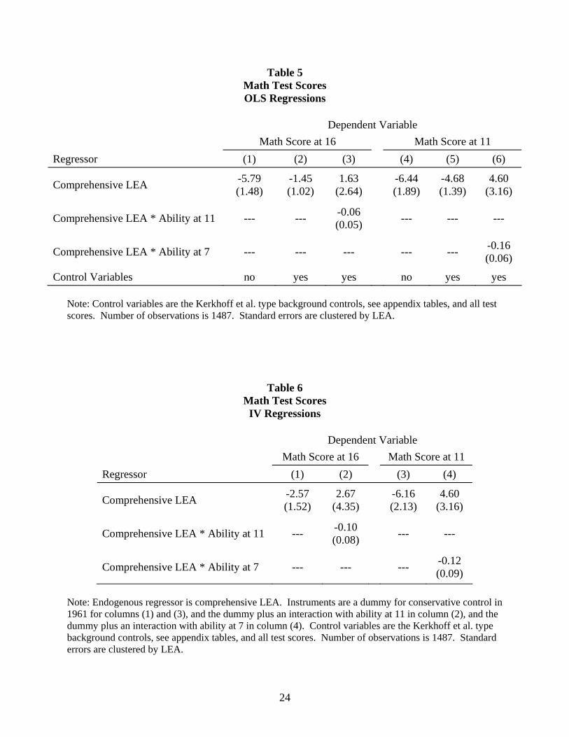
Table 5 displays the results. The raw difference between students in comprehensive and

selective LEAs is 5.8 points. This is smaller than the raw difference between all comprehensive

and selective students. Nevertheless, it is large compared to the variation in test scores between

LEAs, which is 9.1 using all LEAs. Adding control variables in column (2) again lowers the

coefficient to about -1.5, very similar to the finding in table 1 based on comprehensive school

attendance. Furthermore, the interactions with lagged ability in column (3) also suggest similar

distribution effects as in table 4, but these effects are now somewhat smaller in magnitude. Not

surprisingly, the results are also less precise in this much smaller sample. Are the LEA level

results likely more reliable? The results for the math score at age 11 suggest the opposite. These

results are also very close to those in tables 2 and 4. Hence, this strategy is not really any more

convincing than the previous one either.

Finally, we follow the suggestion in Galindo-Rueda and Vignoles (2005) and use political

composition of the county as an instrument for comprehensive status. Our instrument,

conservative control of the county or borough in 1961, predicts comprehensive status very well.

The t-statistic on the instrument in the first stage corresponding to column (1) in table 6 is 32.4.

The IV estimate of the comprehensive effect is -2.6, slightly more negative than the OLS

estimate in column (2) of table 5. We also repeat the specifications interacting ability with

comprehensive status in column (2). In this case, we use the interaction of ability and

conservative control as an instrument for the interaction term. Again, the results are roughly

similar to the OLS results. Moreover, columns (3) and (4) show that we also obtain comparable

results for the age 11 test scores yet again. The instrumental variables strategy also does not

seem to be able to remove the selection bias successfully.

18

Conclusion

We have argued in this paper that the experience in England and Wales provides potentially a

useful experiment to study the impact of comprehensive versus selective schooling. Much of the

research on this issue has adopted popular value added specifications for test score outcomes of

affected and unaffected students. We have argued that a useful specification test for these types

of models is to apply them to students during their primary school years by using age 11 test

scores at the dependent variable, and controlling for age 7 test scores. As long as students do not

fare differently in primary school, depending on whether they end up in a comprehensive or a

selective school in the secondary system, these regressions should show a zero comprehensive

effect if all selection is successfully controlled.

Our results indicate the opposite. Throughout the analysis, we have found rather similar patterns

of results for the age 16 test scores and for the age 11 test scores. We conclude from this that it

is prudent to be cautious about interpreting the age 16 results causally. As long as the age 11

results reflect selection bias, this may also be the case for the age 16 results.

Of course, it is possible to argue that our age 11 results are biased, while the age 16

specifications have removed all selection effects successfully. There are various arguments to

make this case, like the fact that age 7 controls are poorer predictors of age 11 outcomes, the fact

that primary school teaching may differ depending on whether the students are going to take the

11+ exam, etc. We have tried to show that none of these are likely to fully explain the age 11

results.

Nevertheless we agree that it is a possibility that the age 16 results are right and the age 11

results are wrong. However, identification always requires a leap of faith. We are typically

willing to make this leap of faith when a research design seem particularly plausible (as in an

experiment) or when we have prior knowledge or additional evidence that a particular

identification strategy is likely to remove the selection bias successfully. In this case, we have

presented evidence to the contrary: that there is a good case to be made that selection bias exists

in the estimates comparing students in comprehensive and selective schools. Our case does not

have to be ironclad to make us worried about the interpretations in the previous literature.

19

Our worry also extends to studies which do not use the NCDS. Similar value added

specifications have been applied to other data in order to answer this question (for example

Jesson, 2000 using more recent data). While we have not explicitly demonstrated potential

problems with these estimates, we would remain cautious in drawing strong conclusions from a

research design that essentially mirrors that adopted by the studies analyzing the NCDS data.

We conclude that we probably do not know very much about the effect of comprehensive

schooling in Britain, or elsewhere for that matter.

20

References

Benn, Caroline (1971) 1971 Survey of Comprehensive Reorganization Plans and Lists of Comprehensive Schools in England, Wales, and Scotland. Comprehensive Schools Committee.

Comprehensive Schools Committee (1967) Comprehensive Education. Secondary Reorganization in England and Wales. Survey No. 1 1966/7.

Crook, D.R., S. Power, and G. Whitty (1999) The Grammar School Question, London: Institute for Education.

Galindo-Rueda, Fernando and Anna Vignoles (2005) “The heterogeneous effect of selection in secondary schools: Understanding the changing role of ability,” CEE Discussion Paper No. 52.

Griffith, A. (1971) Secondary School Reorganization in England and Wales, London: Routledge & Kegan Paul.

Hanushek, Eric and Ludger Wößmann (2006) “Does Educational Tracking Affect Performance and Inequality? Differences-in-Differences Evidence across Countries,” Economic Journal 116, C63-C76.

Jesson, David (2000) “The Comparative Evaluation of GCSE Value-Added Performance by Type of School and LEA,” University of York Discussion Papers in Economics No. 2000/52.

Kerckhoff, Alan C., Ken Fogelman, David Crook, and David Reeder (1996) Going Comprehensive in England and Wales. A Study of Uneven Change, London: The Woburn Press.

Municipal Yearbook (1962, 1968) London: Municipal Journal Ltd.

Todd, Petra and Kenneth Wolpin (2003) “On the Specification and Estimation of the Production Function for Coginitive Achievement” Economic Journal 113, F3-F33.

Waldinger, Fabian (2006) “Does Tracking Affect the Importance of Family Background on

Students' Test Scores?” mimeographed, London School of Economics

21

Figure 1Shares of Publically Supported Pupils by School Type

0

10

20

30

40

50

60

70

80

90

100

1965 1975 1985 1995

Year

Perc

ent

Comprehensive Grammar Other

22

Table 1 Math Test Scores at 16

OLS Regressions

Regressor (1) (2) (3) (4) (5)

Attends Comprehensive School -7.74 (0.54)

-2.18 (0.35)

-2.07 (0.34)

-1.80 (0.34)

-1.48 (0.37)

Control Variables: Math Test Score at 11 no yes yes yes yes Other Test Scores at 11 no no yes yes yes

Kerkhoff et al. type background controls no no no yes yes

Large set of background controls no no no no yes Number of observations 6734 6734 6734 6734 5747

Note: Control variables are described in Appendix table 1

Table 2 Math Test Scores at 11

OLS Regressions

Regressor (1) (2) (3) (4) (5)

Attends Comprehensive School -8.39 (0.62)

-6.01 (0.52)

-4.91 (0.46)

-3.96 (0.45)

-3.29 (0.45)

Control Variables: Math Test Score at 7 no yes yes yes yes Other Test Scores at 7 no no yes yes yes

Kerkhoff et al. type background controls no no no yes yes

Large set of background controls no no no no yes Number of observations 6734 6734 6734 6734 6223

Note: Control variables are described in Appendix table 2

23

Table 3 Math Test Scores

Dependent Variable Math Test Score at 16 Math Test Score at 11 Estimation Method OLS IV IV OLS IV IV Regressor (1) (2) (3) (4) (5) (6)

Attends Comprehensive School

-1.88 (0.35)

-1.24 (0.36)

-1.28 (0.36)

-4.59 (0.50)

-2.90 (0.62)

-2.91 (0.62)

Math Test Score at 11 0.63 (0.01)

0.73 (0.01)

0.73 (0.01) --- --- ---

Math Test Score at 7 --- --- --- 0.54 (0.01)

1.14 (0.03)

1.14 (0.02)

Instruments: Reading Test Score at 11 no yes yes no no no Other Test Scores at 11 no no yes no no no Reading Test Score at 7 no no no no yes yes Other Test Scores at 7 no no no no no yes

Note: Endogenous regressor is the math test score at 11. Control variables are the Kerkhoff et al. type background controls, see appendix tables. Number of observations is 6734.

Table 4 Math Test Scores OLS Regressions

Dependent Variable

Math Score at 16

Math Score at 11

Regressor (1) (2)

Attends Comprehensive School 3.49 (0.96)

5.66 (1.75)

Comprehensive School * Ability at 11 -0.10 (0.02) ---

Comprehensive School * Ability at 7 --- -0.17 (0.03)

Note: Control variables are the Kerkhoff et al. type background controls, see appendix tables, and all test scores. Number of observations is 6734.

24

Table 5 Math Test Scores OLS Regressions

Dependent Variable Math Score at 16 Math Score at 11 Regressor (1) (2) (3) (4) (5) (6)

Comprehensive LEA -5.79 (1.48)

-1.45 (1.02)

1.63 (2.64)

-6.44 (1.89)

-4.68 (1.39)

4.60 (3.16)

Comprehensive LEA * Ability at 11 --- --- -0.06 (0.05)

--- --- ---

Comprehensive LEA * Ability at 7 --- --- ---

--- --- -0.16 (0.06)

Control Variables no yes yes no yes yes Note: Control variables are the Kerkhoff et al. type background controls, see appendix tables, and all test scores. Number of observations is 1487. Standard errors are clustered by LEA.

Table 6 Math Test Scores

IV Regressions

Dependent Variable Math Score at 16 Math Score at 11 Regressor (1) (2) (3) (4)

Comprehensive LEA -2.57 (1.52)

2.67 (4.35)

-6.16 (2.13)

4.60 (3.16)

Comprehensive LEA * Ability at 11 --- -0.10 (0.08)

--- ---

Comprehensive LEA * Ability at 7 --- ---

--- -0.12 (0.09)

Note: Endogenous regressor is comprehensive LEA. Instruments are a dummy for conservative control in 1961 for columns (1) and (3), and the dummy plus an interaction with ability at 11 in column (2), and the dummy plus an interaction with ability at 7 in column (4). Control variables are the Kerkhoff et al. type background controls, see appendix tables, and all test scores. Number of observations is 1487. Standard errors are clustered by LEA.

25

Appendix Table 1 Summary Statistics for Age 16 Regressions

Variable Number of Obs. Mean Standard

Deviation Math Test Score at 16 6734 42.4 22.4 Attends Comprehensive School 6734 0.547 ---

Control Variables

Math Test Score at 11 6734 44.0 25.8

Other Test Scores

Reading Test Score at 11 6734 47.4 17.8 Verbal Test Score at 11 6734 57.7 23.0 Nonverbal Test Score at 11 6734 54.4 18.4 Design Copy Score at 11 6734 70.3 11.4

Kerkhoff et al. type background controls

Female 6734 0.491 --- Two or more siblings 6734 0.608 --- Twin 6734 0.026 --- No mother figure at 11 6734 0.005 --- No father figure at 11 6734 0.034 --- Father’s occupation at 11: professional 6734 0.055 --- Father’s occupation at 11: intermediate 6734 0.184 --- Father’s occupation at 11: skilled 6734 0.519 --- Father’s occupation at 11: semi-skilled 6734 0.161 ---

continued

26

Appendix Table 1 (continued) Summary Statistics for Age 16 Regressions

Variable Number of Obs. Mean Standard

Deviation Large set of background controls

No father figure at 7 5747 0.020 --- Wales 5747 0.070 --- Borough council 5747 0.353 --- Father unemployed at 11 5747 0.026 --- Mother works at 11 5747 0.629 --- Free meal at school at 11 5747 0.077 --- Family had financial trouble last 12 months at 11 5747 0.091 --- Accommodation rented from council at 11 5747 0.382 --- Child doesn’t share bedroom at 11 5747 0.471 --- Accommodation as bath at 11 5747 0.951 --- Accommodation has indoor lavatory at 11 5747 0.899 --- Has moved 2 or more times since birth at 11 5747 0.355 --- Parents expect child to leave school at min. SLA 5747 0.045 --- Child goes to public library often at 11 5747 0.256 --- Child had contact with criminal justice system betw. age 7 and 11 5747 0.015 --- Missed school for 1 week to 1 month at 11 5747 0.317 --- Missed school for more than 1 month at 11 5747 0.048 --- Mom had health problems between age 7 and 11 5747 0.034 --- Child plans to get job after school 5747 0.196 --- Child plans to go to university after school 5747 0.290 --- Watches TV most of the day at 11 5747 0.848 --- Child attends private school at 11 5747 0.033 --- Child attends special needs school at 11 5747 0.005 --- School size at 11 5747 323.0 139.7 Class size at 11 5747 34.8 7.2 Attended two or more schools by 11 5747 0.454 --- Age group tracked at 11, higher ability track 5747 0.157 --- Age group tracked at 11, intermediate ability track 5747 0.111 --- Age group tracked at 11, lower ability track 5747 0.091 --- Teacher rating of general ability at 11 (score 1-5) 5747 3.06 0.84 Teacher rating of math ability at 11 (score 1-5) 5747 2.97 0.92 Teacher rating of use of books at 11 (score 1-5) 5747 3.20 0.85 Teacher rating of oral ability at 11 (score 1-5) 5747 3.11 0.75 County level proportion hhs in council housing, 1971 5747 0.291 0.090 County level proportion employment manufacturing, 1971 5747 0.355 0.099 County level proportion single parents, 1971 5747 0.089 0.026 County level proportion men who are economically active, 1971 5747 0.607 0.018 County level proportion men born in UK, 1971 5747 0.940 0.052

27

Appendix Table 2 Summary Statistics for Age 11 Regressions

Variable Number of Obs. Mean Standard

Deviation Math Test Score at 11 6734 44.0 25.8 Attends Comprehensive School 6734 0.547 ---

Control Variables

Math Test Score at 7 6734 52.9 24.5

Other Test Scores

Reading Test Score at 7 6734 79.4 22.5 Drawing Test Score at 7 6734 41.4 11.7

Kerkhoff et al. type background controls

Female 6734 0.491 --- Two or more siblings 6734 0.608 --- Twin 6734 0.026 --- No father figure at 7 6734 0.021 --- Father’s occupation at 7: professional 6734 0.053 --- Father’s occupation at 7: intermediate 6734 0.149 --- Father’s occupation at 7: skilled 6734 0.545 --- Father’s occupation at 7: semi-skilled 6734 0.163 ---

continued

28

Appendix Table 2 (continued) Summary Statistics for Age 11 Regressions

Variable Number of Obs. Mean Standard

Deviation Large set of background controls

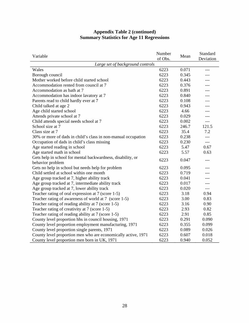
Wales 6223 0.071 --- Borough council 6223 0.345 --- Mother worked before child started school 6223 0.443 --- Accommodation rented from council at 7 6223 0.376 --- Accommodation as bath at 7 6223 0.891 --- Accommodation has indoor lavatory at 7 6223 0.840 --- Parents read to child hardly ever at 7 6223 0.108 --- Child talked at age 2 6223 0.943 --- Age child started school 6223 4.66 --- Attends private school at 7 6223 0.029 --- Child attends special needs school at 7 6223 0.002 --- School size at 7 6223 246.7 121.5 Class size at 7 6223 35.4 7.2 30% or more of dads in child’s class in non-manual occupation 6223 0.238 --- Occupation of dads in child’s class missing 6223 0.230 --- Age started reading in school 6223 5.47 0.67 Age started math in school 6223 5.57 0.63 Gets help in school for mental backwardness, disability, or behavior problem 6223 0.047 ---

Gets no help in school but needs help for problem 6223 0.095 --- Child settled at school within one month 6223 0.719 --- Age group tracked at 7, higher ability track 6223 0.041 --- Age group tracked at 7, intermediate ability track 6223 0.017 --- Age group tracked at 7, lower ability track 6223 0.020 --- Teacher rating of oral expression at 7 (score 1-5) 6223 3.18 0.94 Teacher rating of awareness of world at 7 (score 1-5) 6223 3.00 0.83 Teacher rating of reading ability at 7 (score 1-5) 6223 3.16 0.90 Teacher rating of creativity at 7 (score 1-5) 6223 2.93 0.82 Teacher rating of reading ability at 7 (score 1-5) 6223 2.91 0.85 County level proportion hhs in council housing, 1971 6223 0.291 0.090 County level proportion employment manufacturing, 1971 6223 0.355 0.099 County level proportion single parents, 1971 6223 0.089 0.026 County level proportion men who are economically active, 1971 6223 0.607 0.018 County level proportion men born in UK, 1971 6223 0.940 0.052

29

Appendix Table 3 Treatment and Control LEAs

Selective LEAs Comprehensive LEAs Barrow in Furness Anglesey Blackpool Blackburn Bolton Cardiff Bournemouth Carlisle Brighton Darlington Buckinghamshire Flintshire Burton upon Trent Gateshead Canterbury Isle of Wight Cheshire Leicestershire Dewsbury Luton Dudley Merioneth Eastbourne Montgomeryshire Great Yarmouth Newcastle upon Tyne Halifax Newport Hastings Norwich Ipswich Oldham Leicester Oxfordshire Norfolk Preston Portsmouth Rochdale Solihull Rotherham South Shields Sheffield Southend on Sea Stoke on Trent Southport Swansea Torbay Tynemouth Warley Wallasey Warrington West Bromwich Warwickshire Worcester York