Compound Poisson approximation: a user’s guide

A. D. Barbour1,2 and O. Chryssaphinou2

Universitat Zurich and University of Athens

Abstract.Compound Poisson approximation is a useful tool in a variety of applications, including

insurance mathematics, reliability theory, and molecular sequence analysis. In this paper,we review the ways in which Stein’s method can currently be used to derive bounds on theerror in such approximations. The theoretical basis for the construction of error boundsis systematically discussed, and a number of specific examples are used for illustration.We give no numerical comparisons in this paper, contenting ourselves with references tothe literature, where compound Poisson approximations derived using Stein’s method areshown frequently to improve upon bounds obtained from problem specific, ad hoc methods.

Keywords: Compound Poisson, Stein’s method, Total Variation Distance, KolmogorovDistance.

AMS 1991 Subject Classifications: 60 02, 60C05, 60E15, 60F05, 60K10, 62E17, 92D20

1 Partially supported by Schweizer Nationalfonds Grant 20-50686.972 Partially supported by University of Athens Research Grant 70-4-2558

1

1. Motivation

Many probability models (Aldous, 1989) involve rare, isolated and weakly dependentclumps of interesting occurences. A typical example is that of clusters of extreme events,such as earthquakes of magnitude exceeding 4.0; when one event occurs, several moremay follow in quick succession, before normality returns. Clusters of events can then beexpected to take place almost ‘at random’, according to a Poisson process, in which casethe number of clusters occurring in a given time interval would have a distribution closeto a Poisson distribution Po(λ) with some mean λ, and the sizes of the individual clumpsmight well also be assumed to be approximately independent and identically distributedwith some distribution µ. If these assumptions were precisely true, the total number W ofoccurrences would then have a compound Poisson distribution CP (λ,µ), the distributionof the sum of a random Po(λ)–distributed number of independent random variables, eachwith distribution µ: more formally, CP (λ,µ) is defined by

CP (λ,µ) = L

M∑j=1

Yj

= L

∑i≥1

iMi

,

for any λ > 0 and any probability distribution µ on IN, where (Yj , j ≥ 1) are independent,have distribution µ and are independent also of M ∼ Po(λ); and where (Mi, i ≥ 1) areindependent, with Mi ∼ Po(λµi). The former representation is that which ties in withthe description above. The latter is an equivalent definition, which emphasizes that thenumber of clumps of each size i ≥ 1 itself has a Poisson distribution, and that thesenumbers are independent; this structure can also be useful.

In practice, the assumptions above are usually not satisfied exactly; the clumps mayoccur only approximately as a Poisson process, and the clump sizes may not quite beindependent. If this is the case, and if the CP (λ,µ) distribution is being used to ap-proximate the distribution of W , it is important to know how accurate the approximationreally is. In this paper, we are interested in showing how to quantify this closeness,when W =

∑γ∈ΓXγ is a countable sum of non–negative integer valued random variables

(Xγ , γ ∈ Γ). We review estimates for the distance between L(W ) and CP (λ,µ), for suit-ably chosen λ and µ, with respect to the Kolmogorov distance dK and the total variationdistance dTV , where, for probability distributions P and Q on 6 6 +,

dK(P,Q) := supj≥0|P[0, j] −Q[0, j]|; dTV (P,Q) := sup

A⊂6 6 +

|PA −QA|.

The Xγ are to be thought of as being generally weakly dependent, apart possibly fromsome strong local dependence, but we retain generality and flexibility by avoiding as faras possible making any specific assumptions in this respect.

2

1.1 Insurance.

A simple model of an insurance portfolio assumes a finite number n of insured risks,each of which may lead to a claim with a small probability, independently of all the others.The distribution of the total number N of claims is then well approximated by the Poissondistribution Po(λ), with λ =

∑nj=1 pj , even if the claim probabilities pj are not equal. Fur-

thermore, as observed by Michel (1988) (see also Le Cam, 1965), if all claim amounts areindependent and identically distributed, the difference in terms of total variation distancebetween the distribution of the aggregated claim amount and an appropriate compoundPoisson distribution is no greater than the total variation distance ∆ ≤ λ−1

∑ni=1 p

2i (Bar-

bour and Hall, 1984) between the distribution of the total number of claims N and Po(λ).If the occurrences of claims are weakly dependent, but the claim amounts are still indepen-dent and identically distributed, Goovaerts and Dhaene (1996) have noted that Michel’sobservation can still be applied, and that the new value of ∆, which will usually be largerthan λ−1

∑ni=1 p

2i , because of the dependence, can be estimated using the Stein–Chen

method (Barbour, Holst and Janson, 1992).In many insurance applications, however, there may be strong local dependence be-

tween claim occurrences. For instance, in storm damage insurance, the (rare) single oc-currence of a tornado in a particular town may lead to some random number of claims onthe portfolio. Since the distribution of this number of claims may well depend on the timeof year, the preceding argument, even assuming independent and identically distributedindividual claim amounts, cannot be applied, because the aggregate claim amounts result-ing from occurrences of tornadoes are no longer independent and identically distributed.Despite this, it still seems reasonable to suppose that the distribution of the total numberof claims is close to a compound Poisson distribution in total variation, in which case, ifonce again the individual claim amounts are independent and identically distributed, thedistribution of the aggregated claim amount is itself at least as close in total variation toan appropriate compound Poisson distribution, again by Michel’s observation. To exploitthis idea, if the possibility of substantial local dependence between the random claim num-bers is also to be allowed, it is necessary to have an equivalent of the Stein–Chen method,which quantifies the error in total variation when approximating the distribution of a sumof nonnegative random variables, most of them taking the value zero with high probability,by a compound Poisson distribution. Once such an equivalent has been developed, there isthe further advantage that one can dispense with Michel’s observation and the assumptionof independent and identically distributed individual claim amounts, and prove compoundPoisson approximations to the total claim amount directly.

1.2 Reliability.

We consider a system of n linearly arranged components, having independent lifetimeswith common distribution function F , connected in such a way that the system fails if at

3

least k consecutive components fail. This reliability system is called the Consecutive–k–out–of–n:F (C(k, n :F )) system. Over the last two decades, the C(k, n :F ) and relatedsystems have been extensively studied by many authors. One can find a rich literaturein Chao, Fu and Koutras (1995). The advantages of using such a system are that it hashigher reliability than a series system, but is less expensive to build than a parallel system.It has applications in telecommunication systems, oil pipelines, vacuum systems, computerring networks, spacecraft relay stations, and many other engineering systems.

The reliability of this system — the probability that it has not failed — has beenexactly determined, but the explicit formula is quite complicated, especially if n and k

are large. For this reason, upper and lower bounds for the reliability have been derived.In this context, the Stein-Chen method for Poisson approximation has proved a power-ful tool. The approach is as follows. For any fixed time T , we associate independentBernoulli Be(p) random variables J1, . . . , Jn with the components, where p = 1 − F (T );Ji takes the value 1(0) if the ith component works(fails), i = 1, . . . , n. We then define therandom variable W =

∑n−k+1i=1 Ii, where Ii =

∏i+k−1j=i (1 − Jj) takes the value 1 if all the

components i, i+1, . . . , i+k−1 fail and 0 in all other cases. Clearly, the C(k, n:F ) systemfails if and only if W > 0. Although the components themselves work independently, theindicators Ii are locally dependent, tending to occur in clusters. Nonetheless, the ran-dom variable W is reasonably well approximated by a Poisson distribution Po(λ) withλ =

∑n−k+1j=1 qk, where q = 1−p, provided that p is small. This has been established using

the Stein-Chen “local” approach (Barbour, Holst and Janson (1992, (8.4.2)), Chryssaphi-nou and Papastavridis (1990), Godbole (1991), and Roos (1993)), and the argument worksequally well for more general situations, such as when the failure probabilities may differfrom component to component. However, the probability IP[W = 0] is more accuratelyestimated by using a Poisson approximation for the distribution of the number of clusters,or, alternatively, a compound Poisson approximation to the distribution of W .

Some more complicated problems, which arise in the design of reliable electronic de-vices and in pattern detection, inspired Salvia and Lasher (1990) to consider a planarversion of the above system. They introduce the Two dimensional Consecutive–k–out–of–

n:F (C(k2, n2:F )) system, which consists of n× n components placed on a square grid; itfails if there is a square subgrid of size at least k × k with all its components failed. Theexact reliability of this system is not known, and thus approximations to it are essential.Salvia and Lasher (1990) obtained bounds for the reliability of the system by relating itto certain C(k, n:F ) systems. Koutras, Papadopoulos and Papastavridis (1993) proposedbounds using results of Arratia, Goldstein and Gordon (1989, 1990) using the Stein-Chenmethod for Poisson approximation.

With the same assumptions about the operating behaviour of the components as forthe C(k, n:F ) system, we define the random variable W =

∑n−k+1i,j=1 Iij , where Iij = I[all

4

components in a k × k subgrid with left lowermost component (i, j) are failed]. Then thereliability of the system is just IP[W = 0]. The indicators Iij and Ii′j′ are independentunless | i − i′ |≤ k − 1 and | j − j′ |≤ k − 1 but the local dependence between the Ii,j isnow frequently relatively strong. For example, the conditional probability that Ii+1,j = 1given that Ii,j = 1 is qk, as compared with the unconditional probability of qk

2. Thus the

indicators Ii,j tend to occur in clusters, and the random variable W is best approximatedby a compound Poisson distribution. The reliability IP[W = 0] is then approximated bye−IEN , where N is the number of clusters, rather than by the Poisson approximation e−IEW ,the two quantities differing inasmuch as IEW = CIEN , where C is the expected clustersize : see Barbour, Chryssaphinou and Roos (1995,1996)

1.3 Sequence matching.

Biological systematics has been revolutionized by the discovery of the double helixand the genetic code, and by the development of cheap, fast and automatic sequencingmachines. The degree of relationship between closely related species can now be assessedin terms of the similarity of their genomes. For more distant species, relationship at theDNA level may well have become obscured because too many random mutations haveoccurred since divergence, but functionally vital elements of the amino acid sequencescomposing their proteins are still likely to have been conserved. Thus unusual similaritybetween (parts of) sequences can be used as evidence for relationship. It then becomesimportant to be able to determine what measure of similarity can be interpreted as unusual.

The simplest model is to suppose that two finite sequences x and y of length n fromthe same finite alphabet A (|A| = 4 for DNA, |A| = 20 for amino acid sequences) are to becompared, which, on the null hypothesis of no relation, are each independently composedof letters drawn independently from A with the same probability distribution ν. A measureof relatedness might be the count W =

∑n−mi,j=1 Iij , where

Iij =m∏l=0

I[xi+l = yj+l],

the number of pairs of subsequences of length m+ 1 from the two sequences which exactlymatch, where m is to be suitably chosen. The indicators Iij and Ii′j′ are independentunless either |i− i′| ≤ m or |j − j′| ≤ m, so that dependence between the Iij is in generalweak; however, the conditional probability that Ii+1,j+1 = 1 given that Iij = 1 is typicallysubstantial (at least 1/|A|), so that matching pairs tend to occur in local clusters. Hence acompound Poisson distribution is a suitable candidate for approximating the distributionof W . There are, of course, many generalizations of the model, the most important, forthe purposes of practical algorithms, being to allow some degree of mismatching in thepairs of interest, through insertions and deletions of sequence segments and through thereplacement of one amino acid by another similar one; see Neuhauser (1994, 1996).

5

2. Compound Poisson approximation

2.1 The Poisson process approach.

A first approach to compound Poisson approximation for sums of dependent indicatorsis to proceed by way of Poisson point process approximation. This is a very natural ideain the context of an underlying process consisting of rare, isolated and weakly dependentclumps of events. In such a system, the locations of the clumps, when suitably defined,occur more or less as a Poisson process on the index set Γ, and, if the sizes of the clumpsare added to Γ as an extra index dimension, then the process of clump locations and sizeson Γ× IN is also almost a Poisson process. The typical strategy is to assign a location toeach clump by using exactly one of the indices γ ∈ Γ as the representative of each clump,and to replace W =

∑γ∈ΓXγ by a sum

W =∑γ∈Γ

∑l≥1

lIγl, (2.1)

where Iγl now denotes the indicator of the event that γ is the index of the representative of aclump of size l; thus, for each clump, exactly one of the Iγl takes the value 1, and no index γis representative of more than one clump. Poisson process approximation in total variationto the point process Ξ =

∑γ∈Γ

∑l≥1 Iγlδl, where δl denotes the point mass at l, is then

accomplished by using Stein’s method for Poisson process approximation, and compoundPoisson approximation in total variation to the random variable W =

∑γ∈Γ

∑l≥1 lIγl,

with exactly the same error estimate, follows as a consequence. There have been manysuccessful applications of this approach, a number of which are given in Arratia, Goldsteinand Gordon (1989,1990).

To formulate the results, we introduce some notation. For each (γ, l) ∈ Γ × IN, letB(γ, l) ⊂ Γ× IN be a set containing γ × IN, and set

b1 =∑

(γ,l)∈Γ×IN

∑(β,j)∈B(γ,l)

IEIγlIEIβj ; b2 =∑

(γ,l)∈Γ×IN

∑(β,j)∈B(γ,l)(β,j)6=(γ,l)

IE(IγlIβj); (2.2)

b3 =∑

(γ,l)∈Γ×IN

IE|IEIγl − IEIγl |σ(Iβj ; (β, j) /∈ B(γ, l))|. (2.3)

The set B(γ, l) can be thought of as indexing the immediate neighbourhood of (γ, l), andshould be chosen so that the indicators Iβj , whose indices (β, j) do not belong to it,collectively have little or no influence on the value of Iγl. The degree of influence fromoutside the immediate neighbourhood, aggregated over all (γ, l), is measured by b3. Analternative expression for it is

b3 = IEN∑

(γ,l)∈Γ×IN

wγlIE∣∣∣∣ IP[Iγl = 1 |σ(Iβj ; (β, j) /∈ B(γ, l))]

IP[Iγl = 1]− 1∣∣∣∣ ,

6

where N :=∑

(γ,l)∈Γ×IN Iγl denotes the total number of clumps, and the wγl are theweights IEIγl/IEN . This represents b3 as the product of IEN and a weighted average of ameasure of the dependence of the distribution of Iγl on what happens outside its immediateneighbourhood, the events in σ(Iβj ; (β, j) /∈ B(γ, l)). Local dependence, which should alsobe weak for a Poisson process approximation to be good, is summarized in b2. This quantitycan be interpreted in a similar way, as the product of IEN and a weighted average of theexpected number of further clumps occurring in the immediate neighbourhood of an indexpair (γ, l), conditional on Iγl = 1. Finally, b1 has a similar interpretation, as IEN timesa weighted average, but now of the unconditional expected number of clumps with indexpairs (β, l) ∈ (γ, l)∪B(γ, l); this is a measure of the ‘extent’ of the neighbourhoods, andshould also be small if Poisson process approximation is to be accurate. Thus the choiceof the sets B(γ, l) is critical to the success of the approach.

With these definitions, the following compound Poisson estimate, derived by wayof a Poisson process approximation, can be proved as in Arratia, Goldstein and Gor-don (1990, Section 4.2.1), with improved coefficients of b1 and b2 from Barbour, Holst andJanson (1992, Theorem 10.A).

CPA PP. If W =∑γ∈Γ

∑l≥1 lIγl is as defined above, and λ :=

∑γ∈Γ

∑l≥1 IEIγl = IEN

and µl := λ−1∑γ∈Γ IEIγl, l ≥ 1, then

dTV (L(W ),CP (λ,µ)) ≤ b1 + b2 + b3. (2.4)

By choosing the sets B(γ, l) carefully, very good results can be obtained, as long as λ isnot too large.

There are two drawbacks to the point process approach. First, the identificationof a unique representative for each clump (‘declumping’) is rarely natural, and can posedifficulties. Secondly, if λ is large, the error estimates derived in this way are frequently farfrom accurate, because the error involved in point process approximation in total variationis often much larger than that for compound Poisson approximation to L(W ). However,the point process approach still provides flexible, useful and explicit error estimates forcompound Poisson approximation.

Example A. Let Xij = IiI[Yi ≥ j], 1 ≤ i ≤ n, j ≥ 1, be a double array of indicators, inwhich the Ii ∼ Be (pi) are independent, and the Yi ∼ µ(i) are independent of each otherand of the Ii. Set

W =n∑i=1

∑j≥1

Xij =n∑i=1

IiYi.

‘Declumping’ is easily achieved by using representatives γ ∈ 1, 2, . . . , n × 1, denotedfor short by i, and then defining Iil = IiI[Yi = l] for each i, l. Then λ =

∑ni=1 pi and µl =

7

λ−1∑ni=1 piµ

(i)l , and, taking B(i, l) = i× IN for each i, it also follows that b1 =

∑ni=1 p

2i

and b2 = b3 = 0. The Poisson process estimate CPA PP thus immediately implies that

dTV (L(W ),CP (λ,µ)) ≤n∑i=1

p2i . (2.5)

To illustrate the implications of (2.5), let p(n) be chosen in such a way that p(n)→ 0and np(n)→∞ as n→∞, and consider three choices of the pi = p

(n)i and µ(i) = µ(in).

Case (a). Suppose that p(n)i = p(n) and µ(in) = µ for all i. Then (2.5) gives a total

variation error bound of np(n)2 for approximation by CP (np(n),µ); however, the trueerror is actually much less, being at most p(n).Case (b). Suppose that the p(n)

i and µ(in) are as in Case (a) for 2 ≤ i ≤ n, and that µ issuch that µ1 > 0; suppose also that p(n)

1 = 12 and that µ(1n) = δ1 for all n. Then (2.5)

gives an error estimate of at least 1/4 for approximation by CP (λn,µn), where

λn = (n− 1)p(n) + 12 and µn = λ−1

n (n− 1)p(n)µ+ 12δ1;

here, the true error in fact tends to 0 with n, being of order O(p(n) + [np(n)]−1).Case (c). Suppose that everything is as in Case (b), except that now µ26 6 + = 1, sothat, in particular, µ1 = 0. In this case, the error estimate of order O(1) furnished by (2.5)is of the correct order.

The contrast between Cases (b) and (c) indicates that improving upon the error estimatesfor compound Poisson approximation that are derived using the point process approach islikely to be a delicate matter.

2.2 The direct approach.

If IEW is large but finite, there is advantage to be gained by taking a direct approachby way of Stein’s method for the compound Poisson distribution, introduced in Barbour,Chen and Loh (1992). Here, there is no need to rewrite W =

∑γ∈ΓXγ in ‘declumped’

form. Instead, for each γ, decompose W into non–negative integer valued random variablesin the form

W = Wγ + Zγ + Uγ +Xγ , (2.6)

where, for the representation to be useful, Wγ should be almost independent of (Xγ , Uγ),and Uγ and Zγ should not be too large: the sense in which these requirements are to beinterpreted becomes clear shortly. Such a decomposition is often realized by partitioningthe indices 1, 2, . . . , n into subsets γ, Sγ , Nγ and Tγ , and setting

Uγ =∑β∈Sγ

Xβ and Zγ =∑β∈Nγ

Xβ

8

(Roos, 1994); Sγ contains those Xβ , β 6= γ, which strongly influence Xγ , Tγ those Xβ

whose cumulative effect on (Xγ , Uγ) is negligible, and Nγ the remainder. This procedureis the analogue of the ‘local’ approach to Poisson approximation (Barbour, Holst andJanson (1992), pp 9–10), which is recovered, for 0–1 valued Xγ , by taking Sγ = ∅ andhence Uγ = 0. Define the parameters λ and µ of the canonical approximating compoundPoisson distribution as follows:

Canonical parameters:

λµl =1l

∑γ∈Γ

IEXγI[Xγ + Uγ = l], l ≥ 1;

λ =∑l≥1

λµl =∑γ∈Γ

IE( Xγ

Xγ + Uγ

)I[Xγ + Uγ ≥ 1]

.

(2.7)

Note that, if the Xγ are 0–1 valued and Sγ = ∅, then µ1 = 1 and all other µi are zero, andλ = IEW , all consistent with the simple Poisson approximation.

Then, setting π(γ)jk = jIP[Xγ = j, Uγ = k]/m1γ , j ≥ 1, k ≥ 0, where m1γ = IEXγ ,

define the four following quantities which appear in the error estimates, and which shouldbe small for the estimates to be good:

δ1 =∑γ∈Γ

m1γ

∑j≥1

∑k≥0

π(γ)jk IE

∣∣∣∣ IP[Xγ = j, Uγ = k |Wγ ]IP[Xγ = j, Uγ = k]

− 1∣∣∣∣; (2.8)

δ2 = 2∑γ∈Γ

IEXγdTV (L(Wγ |Xγ , Uγ),L(Wγ))

; (2.9)

δ3 =∑γ∈Γ

IEXγdW (L(Wγ |Xγ , Uγ),L(Wγ))

; (2.10)

δ4 =∑γ∈Γ

IE(XγZγ) + IEXγIEXγ + Uγ + Zγ . (2.11)

In (2.10), the distance dW is the Wasserstein L1 metric on probability measures over 6 6 +:

dW (P,Q) = supf∈Lip1

∣∣∣∣∫ f dP −∫f dQ

∣∣∣∣ ,where Lip1 = f : |f(r)− f(s)| ≤ |r − s|, r, s ∈ 6 6 +.

The quantities δl, 1 ≤ l ≤ 4, can be interpreted as follows. To start with, δ4 is ananalogue of b1 + b2 in (2.2), combining the effects of local dependence and neighbourhoodsize, and it reduces to the corresponding element in the Poisson ‘local’ bounds (Barbour,Holst and Janson, (1.28)) if the Xγ are 0–1 valued and Sγ = ∅. Two points should be

9

noted. First, the two weighted averages are now multiplied by the expectation∑γ∈Γ IEXγ

of W , and not by the expected number λ of clumps. Secondly, in the term∑γ∈Γ

IE(XγZγ) = IEW∑γ∈Γ

w′γ∑l≥1

lIP[Xγ = l]IEXγ

IE(Zγ |Xγ = l),

where the weights w′γ are defined by w′γ := IEXγ/IEW , the average is over conditionalexpectations of Zγ given the value of Xγ , and does not include any contribution from thestrongly dependent Uγ ; the effect of the Uγ is already accounted for in the definition ofthe canonical parameters (2.7).

Each of the quantities δ1, δ2 and δ3 is a measure of the effect of any long range depen-dence on the joint distribution of (Xγ , Uγ), and can be contrasted with b3 in (2.3). In δ2and δ3, it is expressed in terms of the effect on the distribution of the ‘distant’ Wγ exer-cised by the value of (Xγ , Uγ), measured either in terms of total variation or Wassersteindistance. In δ1, the dependence is rewritten in terms of the effect on the distribution of(Xγ , Uγ) exercised by Wγ . All three can be viewed as weighted averages of measures of de-pendence at a distance, multiplied by IEW . For independent Xi, one can take Zi = Ui = 0,for which choice δ1 = δ2 = δ3 = 0, and δ4 reduces to

∑ni=1(IEXi)2.

Remark. The distances d(L(Wγ |Xγ , Uγ),L(Wγ)) appearing in (2.9) and (2.10) are oftenbounded by constructing random variables W 1,i,l

γ and W 2,i,lγ on the same probability space,

for each i ≥ 1 and l ≥ 0, with L(W 1,i,lγ ) = L(Wγ | (Xγ , Uγ) = (i, l)) and L(W 2,i,l

γ ) = L(Wγ),in such a way that W 1,i,l

γ and W 2,i,lγ are close — for instance, so that they coincide with

high probability. In practice, it is often easier to make a coupling of L(Wγ | (Xγ , Uγ , Yγ) =(i, l, y)) and L(Wγ), where Yγ summarizes additional information, for example the exactknowledge of (Iβ , β ∈ Sγ) rather than just the value of Uγ . This causes no extra difficulty,since it is always the case that

IEXγd(L(Wγ |Xγ , Uγ),L(Wγ)) ≤ IEXγd(L(Wγ |Xγ , Uγ , Yγ),L(Wγ)).

In terms of these quantities, the following estimate can be established: see Roos (1994),Barbour and Utev (1999, Theorem 1.9), Barbour (1999, Equations (5.13) and (5.14)).

CPA 1A. There exist constants

HKl = HK

l (λ,µ) ≤ HTVl = HTV

l (λ,µ), l = 0, 1,

which do not involve W in any way, such that, if λ and µ are the canonical parameters,

then

dK(L(W ),CP (λ,µ)) ≤ ε0HK0 + ε1H

K1 ; dTV (L(W ),CP (λ,µ)) ≤ ε0H

TV0 + ε1H

TV1 ;(2.12)

10

in either bound, one can take (i) ε0 = min(δ1, δ2) and ε1 = δ4, or (ii) ε0 = 0 and ε1 = δ3+δ4.

In general, when evaluating δ2 and δ3, it is often possible to compute the distances betweendistributions by means of couplings. Variant (ii), when applied with Zi = 0, gives theanalogue of the Poisson coupling estimate; variant (i) leads to the analogue of the Poissonlocal estimate (Barbour, Holst and Janson 1992, Theorems 1.B and 1.A, respectively).

If approximation by another compound Poisson distribution with parameters λ′ and µ′

is preferred, a similar estimate is available (Barbour 1999, Compound Poisson Estimate 2).One advantage of allowing distributions other than the canonical compound Poisson dis-tribution as approximations is that the canonical distribution may be very complicated,whereas an approximation of the same order may be obtainable with a very simple com-pound Poisson distribution.

CPA 1B. For any choices λ′ and µ′, we have

dK(L(W ),CP (λ′,µ′)) ≤ ε′0H ′K0 + ε′1H′K1 ; dTV (L(W ),CP (λ′,µ′)) ≤ ε′0H ′TV0 + ε′1H

′TV1 ,

(2.13)where H ′Kl = HK

l (λ′,µ′) and H ′TVl = HTVl (λ′,µ′) for l = 0, 1, and where

ε′0 = ε0 + |λm1 − λ′m′1| and ε′1 = ε1 + λm1dW (Q′, Q), (2.14)

with ε0 and ε1 as for CPA 1A; here m1 =∑l≥1 lµl, and the probability measures Q and Q′

on IN are such that Qi = iµi/m1 and Q′i = iµ′i/m′1. In particular, if λ′m′1 = λm1,

then ε′0 = ε0.

Remark. If λ′m′1 = λm1, then one can instead take

ε′1 = ε1 +∑l≥1

l(l − 1)|λ′µ′l − λµl| (2.15)

(Roos, 1994, Theorem 3). The formulae for the elements λµl from the canonical parametersare easy to obtain from (2.7), and the alternative parameters λ′ and µ′ are usually chosenfor their simplicity, so that this quantity is easy to compute.

In order to exploit CPA 1A and CPA 1B, it thus remains to find suitable bounds forHKl (λ,µ) and HTV

l (λ,µ), l = 0, 1. In the Poisson case — µ = δ1 — it is known that

HTV0 (λ, δ1) ≤ min1,

√2/eλ; HTV

1 (λ, δ1) ≤ min1, λ−1, (2.16)

(Barbour, Holst and Janson, Lemma 1.1.1 and Remark 10.2.4). If bounds with similar λ–dependence could also be found for general compound Poisson distributions, the estimatesof CPA 1A and CPA 1B would greatly improve upon the error estimates derived in CPA PP.

11

The reason for this is quite simple. In the constituents δl, 1 ≤ l ≤ 4, of the bounds given inCPA 1A and CPA 1B, as also in b1, b2 and b3 of CPA PP, average measures of dependenceat each location are multiplied by the mean of W or by λ, the mean number of clumps,each of which increases in proportion to the overall size of the system. Bounds of thismagnitude are an intrinsic feature of total variation approximation for Poisson processes,and are thus unavoidable in CPA PP, but, as in the Poisson case, the same need not be trueof total variation approximation to L(W ). In particular, whenever HTV

1 (λ,µ) = O(λ−1)is true, the elements in the estimate CPA 1A involving ε1 can be made independent of thesystem size, since the factor λ−1 neutralizes the growth of the multiplying factor IEW in δ3and δ4: this is particularly advantageous for variant (ii) of the estimates. Unfortunately,the only known analogue of (2.16) for general µ is the bound

HTVl (λ,µ) ≤ min1, (λµ1)−1eλ, l = 0, 1, (2.17)

proved in Barbour, Chen and Loh (1992). This bound can be useful for small λ, but forlarger λ the exponential factor rapidly makes itself felt. What is more, it is shown inBarbour and Utev (1998) that there can be no general analogue of (2.16) in which thebounds decrease with λ.

Placing some restrictions on µ, however, better bounds can be obtained. Under thecondition

iµi ≥ (i+ 1)µi+1, i ≥ 1, (2.18)

it follows that (Barbour, Chen and Loh, 1992)

HTV0 (λ,µ) ≤ min

1,

1√λ(µ1 − 2µ2)

(2− 1√

λ(µ1 − 2µ2)

);

HTV1 (λ,µ) ≤ min

1,

1λ(µ1 − 2µ2)

(1

4λ(µ1 − 2µ2)+ log+2λ(µ1 − 2µ2)

).

(2.19)

Alternatively, if the condition

θ := m−11 (m2 −m1) < 1/2 (2.20)

holds, where m2 :=∑l≥1 l

2µl, then it follows that

HTV0 (λ,µ) ≤ 1

(1− 2θ)√λm1

; HTV1 (λ,µ) ≤ 1

(1− 2θ)λm1, (2.21)

(Barbour and Xia, 1999b), these latter bounds being of exactly the same order in λ asthose of (2.16) for the Poisson distribution. Note that, for the canonical parameters λand µ,

θ =∑γ∈Γ

IE(XγUγ)/∑γ∈Γ

IEXγ (2.22)

12

is a weighted average of the conditional expectations of the excess clump sizes Uγ at γ,given the possible positive values of Xγ ; if the Xγ are indicators and the pairs (Xγ , Uγ)are identically distributed, then θ = IE(Uγ |Xγ = 1).

Neither of the conditions (2.18) and (2.20) allows the approximating compound Pois-son to be too far from a Poisson distribution — indeed, in the latter case, it follows thatm1 < 3/2 and hence that µ1 > 1/2. Nonetheless, there are many applications, for exam-ple in the area of scan statistics, in which a Poisson approximation is a reasonable butcrude first approximation, and approximation by a compound Poisson distribution whichis not too far from the Poisson can be very much better. In such cases, the bounds (2.19)and (2.21) combined with the error estimates given in CPA 1A and CPA 1B can prove ex-tremely effective; see, for example, (3.4), (3.7) and (3.20) below. For Kolmogorov distance,sharper bounds under Condition (2.18) are also available (Barbour and Xia, 1999a):

HK0 (λ,µ) ≤ min

1,√

2eλµ1

; HK

1 (λ,µ) ≤ min

12,

1λµ1 + 1

. (2.23)

If neither (2.18) nor (2.20) holds, there is as yet no simple fix, though the theorems inSection 2.3 frequently make it possible to obtain approximation errors of best asymptoticorder, albeit with unpalatable constants.

Example A (continued). Define Γ = (i, j) : 1 ≤ i ≤ n, j ≥ 1, and use the decomposition(2.6) with Uij =

∑l 6=j Xil and Zij = 0. Then the pair (Xij , Uij) is independent of Wij ,

so that δ1 = δ2 = δ3 = ε0 = 0, and ε1 = δ4 =∑ni=1 p

2i (IEYi)

2; λ =∑ni=1 pi and

µl = λ−1∑ni=1 piµ

(i)l are as before. Then the direct estimate CPA 1A gives

dTV (L(W ),CP (λ,µ)) ≤ HTV1 (λ,µ)

n∑i=1

p2i (IEYi)

2. (2.24)

If Condition (2.20) holds, then in Case (a) the bound (2.21) implies an error estimateof (1 − 2θ)−1m1p(n), of the correct asymptotic order; in Case (b), the error estimate isless than

(1− 2θ)−1m1p(n) + [4(n− 1)m1p(n)]−1,

again of the correct asymptotic order; Case (c) is incompatible with Condition (2.20).If Condition (2.18) holds with µ1 > 2µ2 and m1 < ∞, then in Cases (a) and (b) the

bound (2.19) leads to error estimates which are asymptotically slightly larger, the orderbeing in both cases multiplied by a factor of lognp(n); again, Case (c) is impossible. Ifneither of Conditions (2.18) and (2.20) are satisfied, the error estimate derived from (2.24)using (2.17) becomes rapidly worse as n increases, and is useless if m1 =∞.

Comparison with the Poisson process estimate. If a ‘declumping’ has been achieved, onecan also use it in conjunction with CPA 1A and 1B. If W =

∑γ∈Γ

∑l≥1 lIγl, as in (2.1),

13

with∑l≥1 Iγl ∈ 0, 1 for each γ, decompose W as in (2.6), but with Γ = Γ× IN in place

of Γ, taking

Xγl = lIγl; Uγl = 0; Zγl =∑

(β,j)∈B(γ,l)(β,j)6=(γ,l)

jIβj ; Wγl =∑

(βj)/∈B(γ,l)

jIβj , (2.25)

where B(γ, l) is as for CPA PP. The canonical parameters λ and µ defined using (2.7) areexactly as for CPA PP, and we can take ε0 = δ1 = b∗3 and ε1 = δ4 = b∗1 + b∗2 in CPA 1Aand 1B, where

b∗1 =∑

(γ,l)∈Γ×IN

∑(β,j)∈B(γ,l)

jlIEIγlIEIβj ; b∗2 =∑

(γ,l)∈Γ×IN

∑(β,j)∈B(γ,l)(β,j)6=(γ,l)

jlIE(IγlIβj);

b∗3 =∑

(γ,l)∈Γ×IN

lIE|IEIγl − IEIγl |σ(Iβj ; (β, j) /∈ B(γ, l))|.(2.26)

This gives the following estimate.

CPA 1C. In the setting of CPA PP, for any choices λ′ and µ′, we have

dK(L(W ),CP (λ′,µ′)) ≤ ε′0H ′K0 + ε′1H′K1 ; dTV (L(W ),CP (λ′,µ′)) ≤ ε′0H ′TV0 + ε′1H

′TV1 ,

(2.27)where H ′Kl = HK

l (λ′,µ′) and H ′TVl = HTVl (λ′,µ′) for l = 0, 1, where b∗1, b∗2 and b∗3 are as

defined in (2.26), and where, as in (2.14),

ε′0 = b∗3 + |λm1 − λ′m′1| and ε′1 = b∗1 + b∗2 + λm1dW (Q′, Q). (2.28)

Comparing the error estimate in (2.27) to that of (2.4), note that the quantities b∗tare larger than the corresponding bt, because of the factors j and l. Thus CPA 1C isnever better than CPA PP unless the HTV

l (λ,µ) are small. This is the case under Con-dition (2.20) as soon as λ becomes large, and then CPA 1C is substantially better thanCPA PP; the same is typically true if Condition (2.18) is satisfied. In other circumstances,CPA PP is normally preferable to CPA 1C, and the direct estimates CPA 1A and 1B areonly competitive if a more advantageous decomposition of W as in (2.6) can be found,without using the declumping.

2.3 Improved estimates.

The weakness of the estimates CPA 1A–1C when the HTVl (λ,µ) are not small sug-

gests that modification of the original Stein argument is needed. One such approach wasexploited in Barbour and Utev (1998, 1999).

14

CPA 2A. If W is decomposed as in (2.6), and if λ > 2, µ and δl, 1 ≤ l ≤ 4, are as in (2.7)–

(2.11), then, for any λ′ > 2 and µ′ satisfying λ′m′1 = λm1, and such that∑j≥1 µ

′jrj <∞

for some r > 1 and that µ′ is aperiodic (µ′l 6 6 + < 1 for all l ≥ 2), we have

dTV (L(W ),CP (λ′,µ′)) ≤ (λ′)−1/2ε0S0(µ′) + (λ′)−1ε′1S1(µ′) + IP[W ≤ φ(µ′)λm1]S2(µ′)(2.29)

whenever λ′m′1 ≥ 2(1 − φ(µ′))−1, where 3/4 < φ(µ′) < 1 and Sl(µ′) < ∞, 0 ≤ l ≤ 2,

and where ε0 and ε′1 are as given in (2.14) and CPA 1A.

The detailed way in which φ(µ′) is to be chosen and in which the Sl(µ′) depend on theradius of convergence of the power series

∑j≥1 µ

′jzj and on the nearness of µ′ to being

periodic are explicitly specified in Barbour and Utev (1999). The third term in (2.29) isa penalty incurred in modifying the straightforward Stein argument. Similar estimatesfor Kolmogorov distance are given in Barbour and Utev (1998), under less restrictiveconditions on µ′.

Note that if a ‘declumping’ has been achieved as in (2.1), then CPA 2A can be appliedwith ε0 = b∗3 and ε1 = b∗1 + b∗2, as defined in (2.26), giving the following estimate.

CPA 2B. If W is declumped as in (2.1) and if λ > 2 and µ are as for CPA PP, then, for

any λ′ > 2 and µ′ satisfying λ′m′1 = λm1, and such that∑j≥1 µ

′jrj < ∞ for some r > 1

and that µ′ is aperiodic (µ′l 6 6 + < 1 for all l ≥ 2), we have

dTV (L(W ),CP (λ′,µ′)) ≤ (λ′)−1/2ε0S0(µ′) + (λ′)−1ε′1S1(µ′) + IP[W ≤ φ(µ′)λm1]S2(µ′)(2.30)

whenever λ′m′1 ≥ 2(1 − φ(µ′))−1, where 3/4 < φ(µ′) < 1 and Sl(µ′) < ∞, 0 ≤ l ≤ 2,

and where ε0 = b∗3 and ε′1 is as given in (2.28).

The advantage of CPA 2A over CPA 1B is that good behaviour as λ increases is ob-tained under much less restrictive conditions on µ′ than those of (2.18) and (2.20). Strongrestrictions on the form of µ′ are replaced by requiring the existence of an exponentialmoment and an aperiodic µ, and the latter condition is essential. For fixed aperiodic µ′

having a finite exponential moment, the coefficients of ε0 and ε′1 are of exactly the samesatisfactory λ–order as in the Poisson case (2.16), and, provided that λ is reasonablylarge, the third term in (2.29) may be relatively unimportant. This makes for excellentasymptotic orders in the error estimates. The disadvantage is that the expressions forSl(µ′) given in Barbour and Utev (1999), while explicit, are very complicated, and canbe expected to be quite large in practical applications: thus error estimates of the correctasymptotic order may be obtained at the cost of unreasonably large constant factors. Inthe same way, CPA 2B frequently improves upon CPA PP in the asymptotic order of theerror estimate, at the expense of introducing unwieldy constant factors.

15

Example A (continued). Suppose that∑j≥1 µjz

j has radius of convergence greater than 1and that µ is aperiodic. Take λ′ and µ′ to be the canonical parameters. In Cases (a)and (b), the Sl(µn) are bounded uniformly in n, and φ(µn) is bounded away from 1.Hence, from (2.29), error estimates of order O(p(n) + exp−np(n)α) for some α > 0 areobtained, with Bernstein’s inequality being used to derive the exponential bound for thethird term in (2.29). This is of the ideal order O(p(n)), except when np(n)→∞ very slowlywith n. At first sight, it appears that the same error estimate should also follow in Case (c),contradicting the fact that the true distance in total variation is of order O(1). The reasonwhy this estimate is not obtained in case (c) is that the distribution µn approaches aperiodic limit µ as n→∞, and the Sl(µn) become unbounded.

In situations where asymptotic rates of approximation are of interest, both λ = λn andµ = µn typically vary with n. In such cases, the error estimate given in CPA 2A dependson n not only in the obvious way, through the quantities λ′n, ε0 = ε

(n)0 and ε′1 = ε′1

(n),but also because the Sl(µ′n), l = 0, 1, 2, and φ(µ′n) depend on n through their dependenceon µ′n. This latter dependence is in general quite complicated. However, the followingresult, which is proved in Mansson (1999, Proposition 2.3), is useful in showing that, forasymptotics, a single choice often suffices for the Sl and for φ.

Proposition. Suppose that ν is an aperiodic probability measure on IN, and that the µ′nare such that, for some r0 > 1 and c > 0,

(i) supn≥1

∑j≥1

µ′jnrj0 <∞;

(ii) infn≥1

µjn ≥ cνj for each j ≥ 1.

Then

S∗l := supn≥1

Sl(µ′n) <∞, l = 0, 1, 2, and 3/4 < φ∗ := supn≥1

φ(µ′n) < 1,

and CPA 2A holds for each n, with S∗l and φ∗ in place of Sl(µ′n) and φ(µ′n), whenever

infn≥1 λ′n > 2(1− φ∗)−1.

The proposition can then be combined with the estimate CPA 2A to give good asymptoticrates in a wide variety of problems.

3. Examples

3.1 Runs

A. Success runs

16

The problem of success runs is very well known in the literature, having already beenconsidered by von Mises (1921) in the context of Poisson approximation. It is the simplestprototype for many problems in the general area of reliability and sequence analysis (Ar-ratia, Goldstein and Gordon (1989, 1990), Arratia, Gordon and Waterman (1990)), andgives a good test of the effectiveness of the various compound Poisson approximations.

To formulate the problem, consider the independent identically distributed Bernoullirandom variables ξ1, . . . , ξn , where IP[ξi = 1] = p = 1 − IP[ξ0 = 0], i = 1, . . . , n. We areinterested in compound Poisson approximation to the number of k–runs of consecutive 1’s.In order to avoid trivialities and edge effects, we assume that n > 4k − 3 and we identifyall indices of the form i + nj for j ∈ Z. We define Iγ =

∏γ+k−1i=γ ξi and W =

∑γ∈Γ Iγ ,

Γ = 1, . . . , n, and set ψ := IEIγ = pk. It is clear that the random variable W counts thenumber of locations among the first n at which a run of 1’s of length at least k begins. Itis also clear that runs of 1’s occur in “clumps”; that is, if there is a run of 1’s of length k

beginning at position γ, then with probability p there will also be a run of 1’s of length k

at position γ + 1, with probability p2 a run of length k beginning at position γ + 2 and soforth. This is an example, with average clump size 1 + p + p2 + p3 + . . ., of the “Poissonclumping heuristic” described by Aldous (1989).

We start by applying the Poisson process approach, as in Arratia, Goldstein and Gor-don (1990). Defining the random variable R =

∑γ∈ΓXγ , where Xγ = (1− ξγ−1)Iγ , with

X1 = I1 we observe that R+∏ni=1 ξi counts the number of clumps, and is approximately

Poisson Po(IER) distributed with mean

IER = ψ[(n− 1)(1− p) + 1]

For interesting results, we want IER to be bounded away from 0, which is essentially thecondition that k ≤ log1/p(n(1− p)). Note that if we are interested in the distribution Mn

of the longest of these 1’s runs, then we have IP[Mn < k] = IP[R = 0].The size of each clump minus one is the length by which the associated run of 1’s

exceeds k, and is approximately distributed as a geometric random variable with param-eter p. Furthermore, the clump sizes are almost independent of each other and of thetotal number R of clumps, so that the distribution of W is approximately Poisson Po(IER)compounded by geometric Ge (p), the Polya–Aeppli distribution PA (IER, p): this is equi-valently expressed as CP (λ,µ) with

λ = IER; µl = pl−1(1− p), l ≥ 1. (3.1)

Although a clump size l could take any value between 1 and n, we shall simplify thecalculation by considering only l ∈ L = 1, 2, . . . , [n/2]− k − 1, and declump by definingIγl = (1 − ξγ−1)ξγξγ+1 . . . ξγ+k+l−2(1 − ξγ+k+l−1) for (γ, l) ∈ Γ × L; then the random

17

variable

W ∗ =∑γ∈Γ

∑l∈L

lIγl = W − nn∏i=1

ξi −∑γ∈Γ

n−k∑[n/2]−k

lIγl

satisfiesdTV (L(W ),L(W ∗)) ≤ pn + np(n/2)−2.

Now takeB(γ, l) = (β, j) : j ∈ L, γ − k − j ≤ β ≤ γ + k + l,

and apply the estimate CPA PP. Simple calculations show that

b1 ≤ n(1− p)ψ22 + (2k + 1)(1− p); b2 ≤ 2n(1− p)ψ2; b3 = 0, (3.2)

and hence the error estimate that results from CPA PP is of order O(nkψ2) = O(kψIEW ).We next turn to the direct approximations CPA 1A and 1B, as exemplified in the

thesis of Roos (1993). We define neighbourhoods of dependence for each γ ∈ Γ, takinginto account the dependence structure of the problem:

Sγ = γ − (k − 1), . . . , γ − 1, γ + 1, . . . , γ + k − 1,Nγ = γ − 2(k − 1), . . . , γ − k, γ + k, . . . , γ + 2(k − 1),Tγ = Γ \ γ ∪ Sγ ∪Nγ

Under the above partioning of Γ, we have a decomposition of the random variable W asin (2.6), with

Wγ =∑β∈Tγ

Iβ , Uγ =∑β∈Sγ

Iβ and Zγ =∑β∈Nγ

Iβ .

We observe that |Sγ | = |Nγ | = 2(k− 1) and that Iβ : β ∈ Sγ ∪ γ are independentof Iβ : β ∈ Tγ for each γ ∈ Γ, so that δ2 = δ3 = δ4 = 0. Furthermore, we have∑

γ∈Γ

((IEIγ)2 + IEIγIEUγ + Zγ) = (4k − 3)nψ2;

∑γ∈Γ

IEIγZγ) = 2(k − 1)nψ2,

and thus, by CPA 1A,

dTV (L(W ),CP (λ,µ)) ≤ HTV1 (λ,µ)

∑γ∈Γ

((IEIγ)2 + IEIγIEUγ + Zγ+ IEIγZγ)

= HTV1 (λ,µ)(6k − 5)nψ2,

18

and the canonical parameters λ and µ are as given in (2.7). These can be explicitlycomputed:

λµi = ni−1IEIkI[Uk + Ik] = i= npki−1IP[I1 + . . .+ Ik−1 + Ik+1 + . . .+ I2k−1 = i− 1|Ik = 1]

= npki−1IP[Vk−1 + V ′k−1 = i− 1],

where Vk−1 and V ′k−1 are independent and Ge(p) truncated at k − 1 distributed randomvariables. Evaluating the last probability, we get

λµi =

nψpi−1(1− p)2, if i = 1, . . . , k − 1;i−1nψ2pi−1(1− p) + (2k − i− 2)pi−1(1− p)2, if i = k, . . . , 2k − 2;(2k − 1)−1nψp2k−2, if i = 2k − 1;

λ =2k−1∑i=1

λµi.

Finally, Roos (1993) showed that Condition (2.18) is satisfied if p ≤ 1/3, so that HTV1 (λ,µ)

can be bounded using (2.19): writing M = λ(µ1 − 2µ2) = npk(1 − p)2(1 − 2p), we derivethe error estimate

dTV (L(W ),CP (λ,µ)) ≤

1 ∧ 1M

[1

4M+ log+ 2M

](6k − 5)nψ2. (3.3)

The estimate (3.3), of order O(kψ log(nψ)), is a big improvement over the bound oforder O(nkψ2) obtained by using CPA PP and (3.2), whenever IEW = nψ is at all large.Furthermore, Condition (2.20) is satisfied for p < 1/5, since θ ≤ 2p/(1 − p), and (2.21)then gives the error estimate

dTV (L(W ),CP (λ,µ)) ≤ (6k − 5)ψ(1− p)/(1− 5p), (3.4)

of even better asymptotic order O(kψ). It is shown in Barbour, Chryssaphinou andVaggelatou (1999, (2.9)) that the canonical compound Poisson distribution can be re-placed, using (2.15) , by the Polya–Aeppli distribution PA (nψ(1 − p), p) (see (3.1)), if4kψ(1 − p)/(1 − 5p) is added to the error estimate. The Markov chain approach of Er-hardsson (1999), outlined in Section 3.6, also gives an approximation of the same orderwhen p < 1/5, but with a better constant factor.

If (essentially) no restriction on p is to be imposed, the estimate CPA 2A is stillavailable; this has been applied in Eichelsbacher and Roos (1999, Section 3.1) to give anerror of order O(kψ + exp(−αknψ)) for some αk > 0, with an unspecified constant. Theterm involving the exponential comes from the third term in (2.29). Finally, Barbour andXia (1999b) examined the same problem in the special case where k = 2. Using a much

19

less straightforward argument and a slightly different approximating compound Poissondistribution, they obtained an explicit error estimate of order O(ψ(nψ)−1/2), which issurprisingly even better than the best of the estimates above, which in this case is of orderO(ψ).

B. Increasing sequences

Consider a sequence X1, . . . , Xn of independent random variables with the same con-tinuous distribution F , and the events Xi−r+1 < . . . < Xi of appearances of increasingsequences of length r, for i = r, . . . , n. Pittel (1981) and Revesz (1983) considered thelimiting behaviour of random variables closely related to the number W of appearances ofthe above event in a sequence of n such trials; we shall approximate its distribution by acompound Poisson distribution, using the estimate CPA 1C. This W could well be usedas a test for local dependence in a supposedly random X–sequence, such as the innova-tions in a supposedly GARCH(1,1) process, being used to model a financial time series,or in ARCH and ARMA processes, as well as in quality control: see Wolfowitz (1944) andEngle (1995).

We first define the indicators

Ii = I[Xi−r+1 < . . . < Xi] for i = r, . . . , n,

so that W =∑ni=r Ii, with IE(W ) = (n− r+ 1)ψ and ψ := 1/r!. Then, in order to achieve

a declumping, we define the indicator random variable Ii,k for the event “a k-clump occursat the ith trial”, that is

Ii,k = I[Xi−r > Xi−r+1 < . . . < Xi < . . . < Xi+k−1 > Xi+k], k ≥ 1.

In this definition, it is assumed that there is a doubly infinite sequence of random variablesXi, i ∈ 6 6 , at our disposal, so that edge effects play no role. This simplifies the analysis, butintroduces an error, in that we actually approximate the distribution of a new ‘declumped’random variable W =

∑ni=r

∑k≥1 kIi,k, which is not quite the same as W ; however,

W differs from W only when, in the infinite sequence, either X0 < X1 < · · · < Xr orXn−r+1 < · · · < Xn < Xn+1, and hence

IP(W 6= W ) ≤ 2(r + 1)!

=2ψr + 1

. (3.5)

The indicator Ii,k is dependent only on the random variables Xi−r, . . . , Xi+k, and isthus independent of all the indicators Ij,l for which j + l < i − r or j − r > i + k. Thisobservation leads us to define the neighbourhoods of dependence by

B(i, k) := (j, l) : i− l − r ≤ j ≤ i+ k + r ∩ (1, . . . , n × IN), (3.6)

20

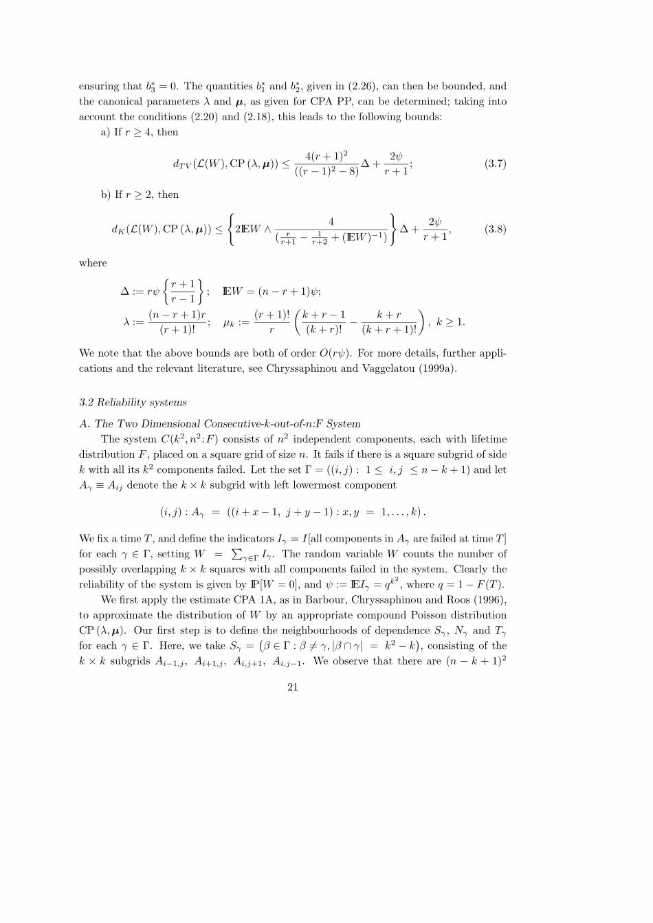
ensuring that b∗3 = 0. The quantities b∗1 and b∗2, given in (2.26), can then be bounded, andthe canonical parameters λ and µ, as given for CPA PP, can be determined; taking intoaccount the conditions (2.20) and (2.18), this leads to the following bounds:

a) If r ≥ 4, then

dTV (L(W ),CP (λ,µ)) ≤ 4(r + 1)2

((r − 1)2 − 8)∆ +

2ψr + 1

; (3.7)

b) If r ≥ 2, then

dK(L(W ),CP (λ,µ)) ≤

2IEW ∧ 4

( rr+1 −

1r+2 + (IEW )−1)

∆ +

2ψr + 1

, (3.8)

where

∆ := rψ

r + 1r − 1

; IEW = (n− r + 1)ψ;

λ :=(n− r + 1)r

(r + 1)!; µk :=

(r + 1)!r

(k + r − 1(k + r)!

− k + r

(k + r + 1)!

), k ≥ 1.

We note that the above bounds are both of order O(rψ). For more details, further appli-cations and the relevant literature, see Chryssaphinou and Vaggelatou (1999a).

3.2 Reliability systems

A. The Two Dimensional Consecutive-k-out-of-n:F System

The system C(k2, n2 :F ) consists of n2 independent components, each with lifetimedistribution F , placed on a square grid of size n. It fails if there is a square subgrid of sidek with all its k2 components failed. Let the set Γ = ((i, j) : 1 ≤ i, j ≤ n− k + 1) and letAγ ≡ Aij denote the k × k subgrid with left lowermost component

(i, j) : Aγ = ((i+ x− 1, j + y − 1) : x, y = 1, . . . , k) .

We fix a time T , and define the indicators Iγ = I[all components in Aγ are failed at time T ]for each γ ∈ Γ, setting W =

∑γ∈Γ Iγ . The random variable W counts the number of

possibly overlapping k × k squares with all components failed in the system. Clearly thereliability of the system is given by IP[W = 0], and ψ := IEIγ = qk

2, where q = 1− F (T ).

We first apply the estimate CPA 1A, as in Barbour, Chryssaphinou and Roos (1996),to approximate the distribution of W by an appropriate compound Poisson distributionCP (λ,µ). Our first step is to define the neighbourhoods of dependence Sγ , Nγ and Tγfor each γ ∈ Γ. Here, we take Sγ =

(β ∈ Γ : β 6= γ, |β ∩ γ| = k2 − k

), consisting of the

k × k subgrids Ai−1,j , Ai+1,j , Ai,j+1, Ai,j−1. We observe that there are (n − k + 1)2

21

possible positions of the k× k subgrid Aγ , of which 4 are corners, 4(n− k− 1) are bordersand the remaining (n − k − 1)2 are interior to Γ, and that then |Sγ | is equal to 2, 3 and4 respectively. Next we take Tγ = (γ ∈ Γ : γ ∩ β = ∅) for all β ∈ Sγ ∪ γ so thatδ2 = δ3 = δ4 = 0, and assign the remaining k × k subgrids to Nγ . Since |Sγ | ≤ 4, we findthat |Sγ | + |Nγ | ≤ (2k + 1)2 − 1. Then W can be written in the form

W = Wγ + Zγ + Uγ + Iγ

as in (2.6), where Uγ =∑γ∈Sγ Iγ , Zγ =

∑γ∈Nγ Iγ and Wγ =

∑γ∈Tγ Iγ .

We now compute the value of δ4 from (2.11), obtaining∑γ∈Γ

(IEIγ)2 = (n− k + 1)2ψ2,

∑γ∈Γ

IEIγIEUγ + Zγ =∑γ∈Γ

∑β∈Sγ∪Nγ

IEIγIEIβ ≤ (n− k + 1)2((2k + 1)2 − 1)ψ2,

∑γ∈Γ

IEIγZγ =∑γ∈Γ

∑β∈Γbγ

IEIγIβ

≤ (n− k + 1)2ψ2

((8k − 4)ψ + 4

(k−1∑r=1

k−1∑s=1

qk2−rs +

k−2∑s=1

qk2−ks

)),

where the complicated sums arise because of the differing overlaps possible between twok × k squares.

Next we compute the canonical parameters from (2.7), obtaining

λµr =1r

∑γ∈Γ

IE

IγIIγ +

∑β∈Sγ

Iβ = r

=

1r

n−k+1∑i=1

n−k+1∑j=1

IEIijI[Iij + Ii,j−1 + Ii−1,j + Ii,j+1 + Ii+1,j = r]

= r−1ψ4π1(r) + 4(n− k − 1)π2(r) + (n− k − 1)2π3(r)

(3.9)

for r = 1, . . . , 5, and λ =∑5r=1 λµr, where

π1(r) = IP

∑β∈Sγ

Iβ = r − 1|Iγ = 1

= IP[Bi(2, qk) = r − 1] for the corner indicators,

π2(r) = IP

∑β∈Sγ

Iβ = r − 1|Iγ = 1

= IP[Bi(3, qk) = r − 1] for the border indicators,

π3(r) = IP

∑β∈Sγ

Iβ = r − 1|Iγ = 1

= IP[Bi(4, qk) = r − 1] for the interior indicators.

22

Hence, applying the approximation CPA 1A, we have

dTV (L(W ),CP (λ,µ))

≤ HTV1 (λ,µ)(n− k + 1)2ψ

((4k2 + 12k − 3)ψ + 4

(k−1∑r=1

k−1∑s=1

qk2−rs +

k−2∑s=1

qk2−ks

)).

(3.10)In reliability applications, it is usual to suppose that λ ≤ λm1 = (n − k + 1)2ψ is smalland the reliability high, in which case the bound HTV

1 (λ,µ) ≤ eλ from (2.17) is adequate.In the above example, the computation of λ and µ is not very complicated, since

we have only to calculate 5 terms, and the resulting error estimate is uniformly of orderO(q2k−1) in λ ≤ 1. This provides an improvement on the order O(qk) obtainable by us-ing the Poisson “local”approach, by the factor O(qk−1). Bigger improvements still couldbe obtained by expanding the set Sγ , but at the cost of more complicated calculationsneeded to determine λ and µ. The same approach is still valid for the case of unequalfailure probabilities, when computer algebra can be used to evaluate the canonical pa-rameters. From tables (see Barbour, Chryssaphinou and Roos (1996)), one can see thatthese error estimates are mostly comparable to or better than those presented by Fu andKoutras (1994), though, for k = 2, the Stein-Chen method is not good in either the Poissonor the compound Poisson approach.

For larger λ, relevant for reliability calculations if the system tolerates up to a largenumber m of failed k × k squares before it collapses, note that

λ(m2 −m1) =5∑r=1

r(r − 1)λµr ≤ 4qkλm1,

so that θ ≤ 4qk. Thus, from (2.21), we can take (n−k+1)2ψHTV1 (λ,µ) = (1−8qk)−1, pro-

vided that 8qk < 1, yielding an error estimate which is still of asymptotic order O(q2k−1).If 8qk ≥ 1 and λ is large, a larger neighbourhood Sγ is needed, if accurate approximationis to be achieved, together with the asymptotically sharper estimate of CPA 2A. For thelatter, a bound on IP[W ≤ φIEW ] for φ < 1 is also required; Janson’s (1990) inequalityshows for instance that here

IP[W ≤ φIEW ] ≤ exp−αIEW/(1 + 4k2qk)

for some α = α(φ) > 0: see Eichelsbacher and Roos (1999, Section 3.3).

B. Multiple failure mode systems

Reliability systems which are subject to more than one type of failure are also ofinterest; see Barlow et al. (1963), Ross (1979), Satoh et al. (1993) and Koutras (1997). The

23

system that we discuss here is also a generalization of consecutive–k–out–of–n:F systemC(k, n:F ), but in a different direction from that of C(k2, n2 :F ). We consider a systemconsisting of n linearly arranged components, in each of which any one of r defects maybe present. The system fails if, for any 1 ≤ i ≤ r, at least ki consecutive componentshave the defect of type i. We denote such a system by C(k1, . . . , kr;n:F ). With the ncomponents, we associate the sequence of random variables X(n) = X1, . . . , Xn takingvalues in A = 0, 1, . . . , r, assuming it to be generated by a stationary Markov chain. Thestate 0 denotes a correctly functioning component, while i denotes a component defectof type i. Such a model can arise as the equilibrium distribution of a reversible nearestneighbour birth and death process, in which a correctly functioning component can becomedefective, or a defective component return to normal working (for example, after repair),with suitably chosen rates depending only on the states of the immediately neighbouringcomponents: see, for example, Preston (1973). In Chryssaphinou and Vaggelatou (1999b),this model is successfully analyzed by using CPA 1C and a declumping. The techniquesrequired are more complicated than those used above, because of the Markov dependence,and are similar in spirit to those that we use in Section 3.4, when counting the occurrencesof copies of a word in a string of letters. The error bounds that they obtain are of orderO(ψ log(1/ψ) max1≤i≤r ki), where ψ =

∑ri=1 ψi and ψi = IP[X1 = X2 = · · · = Xki = i],

and where the constants implicit in the order depend on the transition matrix of theunderlying Markov chain.

C. Connected-s Systems

Many reliability systems can be represented as graphs G(V,E) with V a set of ver-tices (machines) and E a set of edges (connections) between them; see Chen, Hwang andLi (1993). Here, we suppose that the n vertices are independently subject to failure, withprobabilities qi, 1 ≤ i ≤ n. The system has a collection of s–vertex ‘sensitive’ subsets, oftenminimal cut sets in the underlying graph, and the system fails if there are at least m suchsubsets with all vertices failed. The Two Dimensional Consecutive–k–out–of–n:F systemis a particular example of a connected–k2 system.

Let Γ denote the set of all sensitive sets and γ = (k1, . . . , ks) its typical element,where k1, . . . , ks are the indices of the s vertices. Set Iγ = I[all vertices in the set γ arefailed], and W =

∑γ∈Γ Iγ ; then the reliability of the system is equal to IP [W ≤ m− 1],

and IEW =∑γ∈Γ

∏i∈γ qi. To define neighbourhoods of dependence, we first specify the

minimum number R of items in common to α and γ when α ∈ Sγ . The possible choices ofR are 1, 2, . . . , s− 1. Note that the choice of R = s leads to the Poisson “local” approach.

24

For 1 ≤ R ≤ s− 1, we define the sets:

Sγ(R) = α ∈ Γ \ γ : |α ∩ γ| = r, r = R, . . . , s− 1;Nγ(R) = β : |β ∩ α| ≥ 1 for some α ∈ γ ∪ Sγ(R) \ γ ∪ Sγ(R);Tγ(R) = Γ \ γ ∪ Γvsγ (R) ∪ Γbγ(R).

With the above definitions, and after some computations, CPA 1A implies that

dTV (L(W ),CP (λ(R),µ(R))) ≤ HTV1 (λ(R),µ(R))Q(R)qs−R+1

max IEW, (3.11)

whereQ(R) = 1 + max

γ∈Γ|Sγ(R)|+ 2 max

γ∈Γ|Nγ(R)|

and qmax is the largest failure probability of an individual item.Thus, for equal q’s, if |Γ| is large and q small, but IEW = |Γ|ψ is of order 1, where

ψ := qs, compound Poisson approximation is reasonable with R = 1 if Q(1) is muchless than |Γ|. If, instead, IEW is large, the approximation CPA 2A can be used to showthat the error in compound Poisson approximation is of order ψQ(1) + IP[W ≤ φIEW ] forsuitable φ < 1, and Janson’s (1990) inequality can be used to bound the latter probability.However, if the structure of Sγ(1) is complicated, it may be difficult to compute thecanonical parameters, either numerically or by using computer algebra. In such cases, alarger value of R and correspondingly smaller Sγ(R) can be chosen, which will however givean error estimate of higher order: we adopted this strategy in the C(k2, n2:F ) example,taking R = k2 − k. Finally, we note that the Poisson estimate is typically poorer thanthe compound Poisson estimates, but that Poisson approximation may be much easier toachieve.

The above general approach is illustrated in Barbour, Chryssaphinou and Roos (1996),where the reliability of a model called “The double pipeline” is approximated by an ap-propriate compound Poisson using CPA 1A.

3.3 Scan statistics.

A. Two dimensional scan statistics

As an example of the application of compound Poisson approximation to scan statis-tics, we take the two dimensional discrete scan statistic which was applied by Glaz (1996)to the problem of detecting minefields: see also Chen and Glaz (1996). Other applicationsare to be found in Glaz et al. (1994) and in Barbour and Mansson (1999).

A two dimensional rectangular region R = [0, L1] × [0, L2] is inspected for theoccurrence of certain events. Fix n1, n2 ≥ 1, and divide R into n1n2 subregions

Jl1,l2 := [(l1 − 1)h1, l1h1]× [(l2 − 1)h2, l2h2] , 1 ≤ li ≤ ni,

25

each of size h1 × h2, where hi = Li/ni; set Γ = (i, j) : 1 ≤ i ≤ n1 − k1 + 1, 1 ≤ j ≤n2−k2 + 1. For γ ∈ Γ, let the random variable Yγ count the number of events that occurin the subregion Jγ . Set Bi,j = (l1, l2) : i ≤ l1 ≤ i + k1 − 1, j ≤ l2 ≤ j + k2 − 1, anddefine the random variable

Sγ =∑β∈Bγ

Yβ , γ ∈ Γ,

which counts the total number of events in the rectangular subregion Bγ of R, whichconsists of k1k2 adjacent smaller subregions. If Sγ exceeds a level m , then we will saythat m events are clustered within the region. Finally, the two dimensional discrete scanstatistic is defined by

Sk = maxSγ ; γ ∈ Γ, k = (k1, k2)

It is of interest to test the null hypotheses of randomness under which it is assumed thatthe Yβ are independent distributed according to a binomial distribution with parametersN and p0 versus the alternative that they are distributed according to a binomial withparameters N and p1, with p1 > p0.

In order to deal with the testing procedure, an accurate approximation for the distri-bution IP(Sk ≥ m) is necessary. A compound Poisson approximation is used for this. Toderive one, we associate the random variable Sk with the random variable

W =∑γ∈Γ

Iγ , where Iγ = I[Sγ ≥ m].

Clearly, the random variable W counts the number of sets of k1×k2 rectangular subregionsin which at least m events occur. Thus we have

IP(W ≥ 1) = IP(Sk ≥ m).

Assuming a Bernoulli model for the number of events in each h1 × h2 subregion, weobserve that the problem of approximating L(W ) by a compound Poisson distribution canbe approached in very much the same way as the two dimensional consecutive k-out-of-n:Fsystem C(k2, n2:F ). In fact, C(k2, n2:F ) is then a particular case of the two dimensionaldiscrete scan statistic, with k1 = k2 = k, n1 = n2 = n and m = k2. The extra generalityin the choices of dimensions k and n makes essentially no difference to the argument, butallowing m < k1k2 is a significant change, since, as m becomes smaller, the dependencebetween neighbouring k1×k2 sets decreases more slowly with decreasing degree of overlap.Thus, in the notation of Section 3.2(C), a large choice of R such as k1k2 − maxk1, k2may no longer give an adequate approximation. In principle, the choice R = 1 would begood, but the computation of µ(R) may only be feasible using a computer. If the Bernoullimodel were replaced by the more general Binomial model, an analogous approach couldstill be used, though the computation of µ(R) would become still more involved.

26

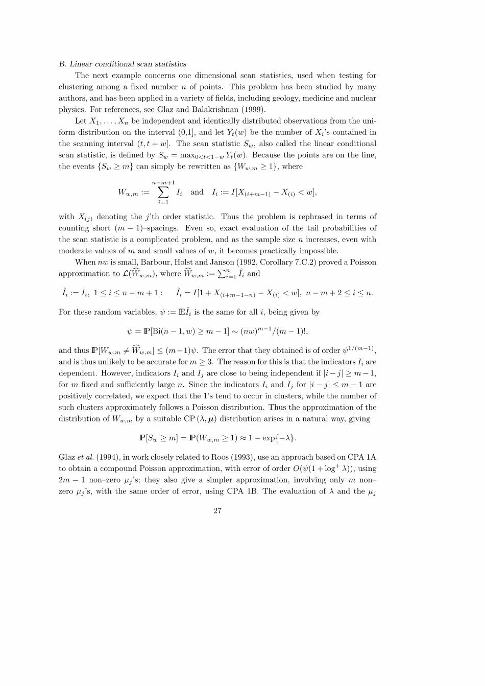
B. Linear conditional scan statistics

The next example concerns one dimensional scan statistics, used when testing forclustering among a fixed number n of points. This problem has been studied by manyauthors, and has been applied in a variety of fields, including geology, medicine and nuclearphysics. For references, see Glaz and Balakrishnan (1999).

Let X1, . . . , Xn be independent and identically distributed observations from the uni-form distribution on the interval (0,1], and let Yt(w) be the number of Xi’s contained inthe scanning interval (t, t + w]. The scan statistic Sw, also called the linear conditionalscan statistic, is defined by Sw = max0<t<1−w Yt(w). Because the points are on the line,the events Sw ≥ m can simply be rewritten as Ww,m ≥ 1, where

Ww,m :=n−m+1∑i=1

Ii and Ii := I[X(i+m−1) −X(i) < w],

with X(j) denoting the j’th order statistic. Thus the problem is rephrased in terms ofcounting short (m − 1)–spacings. Even so, exact evaluation of the tail probabilities ofthe scan statistic is a complicated problem, and as the sample size n increases, even withmoderate values of m and small values of w, it becomes practically impossible.

When nw is small, Barbour, Holst and Janson (1992, Corollary 7.C.2) proved a Poissonapproximation to L(Ww,m), where Ww,m :=

∑ni=1 Ii and

Ii := Ii, 1 ≤ i ≤ n−m+ 1 : Ii = I[1 +X(i+m−1−n) −X(i) < w], n−m+ 2 ≤ i ≤ n.

For these random variables, ψ := IEIi is the same for all i, being given by

ψ = IP[Bi(n− 1, w) ≥ m− 1] ∼ (nw)m−1/(m− 1)!,

and thus IP[Ww,m 6= Ww,m] ≤ (m−1)ψ. The error that they obtained is of order ψ1/(m−1),and is thus unlikely to be accurate form ≥ 3. The reason for this is that the indicators Ii aredependent. However, indicators Ii and Ij are close to being independent if |i− j| ≥ m− 1,for m fixed and sufficiently large n. Since the indicators Ii and Ij for |i− j| ≤ m− 1 arepositively correlated, we expect that the 1’s tend to occur in clusters, while the number ofsuch clusters approximately follows a Poisson distribution. Thus the approximation of thedistribution of Ww,m by a suitable CP (λ,µ) distribution arises in a natural way, giving

IP[Sw ≥ m] = IP(Ww,m ≥ 1) ≈ 1− exp−λ.

Glaz et al. (1994), in work closely related to Roos (1993), use an approach based on CPA 1Ato obtain a compound Poisson approximation, with error of order O(ψ(1 + log+ λ)), using2m − 1 non–zero µj ’s; they also give a simpler approximation, involving only m non–zero µj ’s, with the same order of error, using CPA 1B. The evaluation of λ and the µj

27

was accomplished using the clumping heuristic of Aldous (1989). Huffer and Lin (1997)suggested an alternative compound Poisson approximation.

3.4 Occurrences of a word in a sequence of letters

Let Ξi, i ≥ 0 be independent and identically distributed random variables takingvalues in a set (alphabet) Ω = ω1, . . . , ωq, q ≥ 2, with probabilities ps = IP[Ξi = ωs],s = 1, . . . , q, i ≥ 0. Let A = α1 . . . αk be a fixed string or word of length k. Wedefine the random variable W which counts the overlapping appearances of the word A

in the sequence Ξ1, . . . ,Ξn. Chryssaphinou and Papastavridis (1988b), using generatingfunctions and combinatorial arguments, proved that the random variable W converges indistribution to a compound Poisson distribution under quite general conditions. Barbour,Holst and Janson (1992) examined the accuracy of Poisson approximation for L(W ) takinginto account the set of periods (see Theorem 8.F). In Example 10.4.2 of the same reference,the case of small periods was examined using a compound Poisson approximation, theaccuracy of which is always much better. Applying CPA PP, together with combinatorialarguments based on the set of principal periods of A, Chryssaphinou, Papastavridis andVaggelatou (1999) obtained an upper bound on the total variation distance between L(W )and an appropriate compound Poisson distribution, but of the same accuracy as thatobtained by Barbour, Holst and Janson (1992). As we shall see later, we can obtainsharper error estimates.

This model has been used to solve problems which arise in many areas. In particular,for a finite sequence Ξ1, . . . ,Ξn of letters taken from the alphabet A,C,G, T, the abovementioned results have proved useful for determining critical values for test statistics in theanalysis of DNA sequences. For more literature see Arratia, Goldstein and Gordon (1989,1990), Arratia, Martin, Reinert and Waterman (1996), Barbour, Holst and Janson (1992)and Waterman (1995).

The assumption of independent Ξi is not a good one for DNA sequences. In whatfollows, we show how to derive compound Poisson approximation for sequences modelledby Markov chains, as in Schbath (1995). We assume that the finite sequence Ξ(n) =Ξ1, . . . ,Ξn of random variables, taking values in the alphabet A = A,C,G, T, arisesfrom a stationary realization of an irreducible, aperiodic, homogeneous Markov chain onthe finite state space A; the more general case of an m–order chain can be treated as afirst–order chain on Am. Let Π(αi, αi+1) denote the first order transition probabilities ofthe chain, and π(αi) the invariant probability of αi.

Define the indicator random variables Iγ , with γ ∈ Γ = 1, . . . , n − k + 1, by Iγ =I[Ξγ = α1, . . . ,Ξγ+k−1 = αk]; then W =

∑γ∈Γ Iγ . We say that A has period p if αi = αi+p

for all i = 1, . . . , k− p, and let P(A) denote the set of periods of A. We also define the setof “principal periods” P ′(A) of A, consisting of the minimal period and of those which are

28

not a multiple of it.Schbath (1995), applying CPA PP, proved that if the IEW are bounded as n → ∞,

then L(W ) can be approximated by a compound Poisson distribution. Her argument runsmuch as follows. First, replace W by a random variable W ∗ which is easier to analyze,defined using the entire doubly infinite stationary sequence Ξi−∞≤i≤∞. Set

Iγl := I[ an l−clump of A′s starts at γ in the infinite sequence]; W ∗ :=∑γ∈Γ

∑l≥1

lIγl.

An l–clump consists of exactly l overlapping occurrences of A, whose union does not overlapany preceding or subsequent occurrence of A. Only the sequence Ξ(n) is observable inpractice, and the definition of Iγl may involve ξi for indices i /∈ 1, 2, . . . , n, so that we areactually interested in the random variable W rather than W ∗. However, W 6= W ∗ only ifa copy of A in the infinite sequence overlaps one of the ends of the interval 1, 2, . . . , n,so that

dTV (L(W ),L(W ∗)) ≤ IP[W 6= W ∗] ≤ 2(k − 1)ψ, (3.12)

where

ψ := IEIγ = π(A) = π(α1)k−1∏i=1

Π(αi, αi+1).

The bound (3.12), of order kψ, is no larger than other terms in the later estimates. Fur-thermore,

IEIγl = (1− L)2Ll−1ψ where L =∑

p∈P′(A)

p∏i=1

Π(αi, αi+1), (3.13)

so that IEW ∗ = (n− k + 1)ψ = IEW .In order to apply CPA PP to W ∗, we begin by defining the neighbourhoods B(γ, l).

In doing so, we introduce an integer r which determines their size, and which can then bechosen to minimize the estimates obtained. Denote by Z(γ, l) the set which contains thepositions of the letters defining the random variable Iγl. We say that the indices (γ, l) and(β, j) are not neighbours if the respective Z(γ, l) and Z(β, j) are separated by at least rpositions, r > 0. Then the neighbourhood Br(γ, l) is given by

Br(γ, l) = (β, j) : −(j + 2)k − r ≤ β − γ ≤ (l + 2)k + r ∩ Γ× IN.

With the above neighbourhoods, computing the quantities (2.2), one obtains (Schbath,1995)

b(r)1 ≤ 2(n− k + 1) (kψ + (2k + r + 1)ψ∗)ψ∗

29

andb(r)2 ≤ 2

πinf(n− k + 1) (kψ + (r − k + 1)ψ∗) +

4π(α1)

(n− k + 1)kψ2,

whereψ∗ =

∑l≥1

IEIγl = ψ(1− L)

and πinf := mina∈A π(a). The long range dependence term b3 of (2.3) can be boundedusing the geometric ergodicity of the Markov chain ξi, Schbath (1995) showing thatb(r)3 = O(n2ρr) for some 0 ≤ ρ < 1. Hence, combining CPA PP with (3.12) through the

triangle inequality, it follows that

dTV (L(W ),CP (λ,µ)) ≤ C1n(k + r + 1)ψ2 + C2n2ρr + 2kψ, (3.14)

where the quantities C1 and C2 are of order O(1), the parameters λ and µ are given by

λµl = (n− k + 1)IEIγl; λ = (n− k + 1)ψ(1− L),

and r can be chosen at will.To illustrate the possible asymptotics, let n = nm, A = Am and k = km all depend on

m ≥ 1, in such a way that ψm := π(Am)→ 0 as m→∞. Note that the quantities ψ and ψ∗

are typically geometrically small as functions of k, so that if the mean IE(Wm) = nmψmis kept bounded then km/ log nm stays bounded away from 0 and ∞. Taking r = rm =3 lognm/ log(ρ−1), the error estimate (3.14) is then of order O(ψm log(ψ−1

m )).For the same sequence of words Am, one could instead count the number of copies

of Am appearing in a sequence of letters from the Markov chain of length growing fasterwith m; for example, nm = [ψ−cm ], for any fixed c > 1. In this case, the error esti-mate (3.14) is of order O(ψ2−c

m log(ψ−1m )), which is not even small with m if c ≥ 2. Here

we see the advantage of the improved compound Poisson estimates. If we again takerm = 3 log nm/ log(ρ−1), the estimate (2.30) can be computed to be of order

ψm log(ψ−1m ) + IP[W ≤ φIEW ], (3.15)

for some φ < 1, and, for c > 1, the regenerative structure of the finite Markov chain canbe used to show that the latter term is of smaller order. Hence the improved estimateCPA 2A yields a much better asymptotic order for c > 1 than does CPA PP, by a factorof ψc−1

m .For small enough values of L, Conditions (2.18) and (2.20) are satisfied: Condi-

tion (2.18) if L ≤ 1/2, allowing (2.27) to be applied using the bounds (2.19) and (2.23), andCondition (2.20) if L < 1/5, in which case (2.27) can be applied with the bounds (2.21).

30

Details and some numerical examples are given in Barbour, Chryssaphinou and Vaggela-tou (2000, Section 3). The Markov chain approach of Erhardsson (1999) (see Section 3.6)can also be applied. The error estimates obtained from his theorems are not quite soexplicit as those derived from (2.27), but they are of comparable accuracy when IEW issmall, and of similar order O(ψm log(ψ−1

m )) in the asymptotic setting considered above.Erhardsson (1997) also considers the number of appearances of words from a prescribedset of words A(i), 1 ≤ i ≤ l; see also Chryssaphinou et al. (2000).

Reinert and Schbath (1998) consider the joint distribution of the numbers of copies ofeach of a finite set of words in a sequence of n letters, Their approximations are expressedin terms of independent compound Poisson distributions, and are valid only under a hy-pothesis which restricts the possible overlapping of clumps of a single word with clumpsof another. They do so by applying CPA PP. This is an example of the generality andusefulness of the point process approach: as yet, there is no bivariate analogue of the directcompound Poisson approach to use as an alternative.

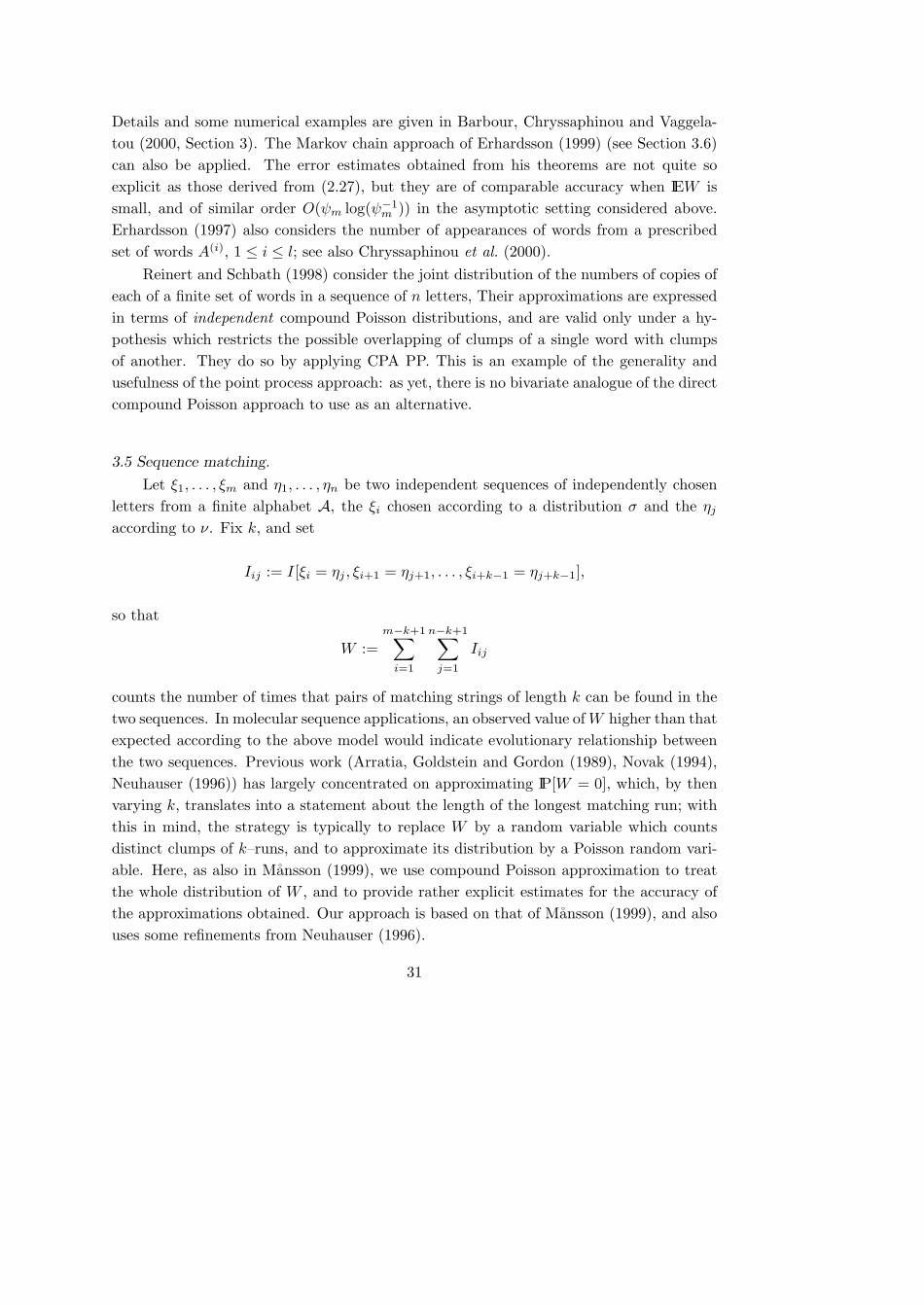
3.5 Sequence matching.

Let ξ1, . . . , ξm and η1, . . . , ηn be two independent sequences of independently chosenletters from a finite alphabet A, the ξi chosen according to a distribution σ and the ηjaccording to ν. Fix k, and set

Iij := I[ξi = ηj , ξi+1 = ηj+1, . . . , ξi+k−1 = ηj+k−1],

so that

W :=m−k+1∑i=1

n−k+1∑j=1

Iij

counts the number of times that pairs of matching strings of length k can be found in thetwo sequences. In molecular sequence applications, an observed value ofW higher than thatexpected according to the above model would indicate evolutionary relationship betweenthe two sequences. Previous work (Arratia, Goldstein and Gordon (1989), Novak (1994),Neuhauser (1996)) has largely concentrated on approximating IP[W = 0], which, by thenvarying k, translates into a statement about the length of the longest matching run; withthis in mind, the strategy is typically to replace W by a random variable which countsdistinct clumps of k–runs, and to approximate its distribution by a Poisson random vari-able. Here, as also in Mansson (1999), we use compound Poisson approximation to treatthe whole distribution of W , and to provide rather explicit estimates for the accuracy ofthe approximations obtained. Our approach is based on that of Mansson (1999), and alsouses some refinements from Neuhauser (1996).

31

In order to simplify the canonical parameters (2.7) of the approximating compoundPoisson distribution, we work instead with the random variable

W ′ :=m∑i=1

n∑j=1

Iij ,

derived from the ξ- and η-sequences by using the ‘torus convention’ ξi+m = ξi, ηj+n = ξjfor all i, j ∈ 6 6 . Since

0 ≤W ′ −W =m∑i=1

n∑j=n−k+2

Iij +m∑

i=m−k+2

n−k+1∑j=1

Iij ,

it is immediate that

dTV (L(W ),L(W ′)) ≤ (m+ n− k + 1)(k − 1)ψ, (3.16)

where ψ := pk and we assume that 0 < p :=∑α∈A σανα < 1. The random variable W ′

has expectationIEW ′ = mnpk,

and we are typically interested in values of k less than, say, 2 log(mn)/log(1/p), so thatIEW ′ is not extremely small. In order to construct a suitable decomposition of the formW ′ = Iij+Uij+Zij+Wij , as in (2.6), we note that the indicators most strongly dependenton Iij are those of the form Ii+l,j+l with |l| ≤ k − 1, so we take

Uij =∑

1≤|l|≤k−1

Ii+l,j+l

and

Zij =

∑(r,s)∈Nij

Irs

− Iij − Uij ,where

Nij = (r, s); min|r − i|, |s− j| ≤ 2(k − 1).

This yields W ′ = Iij + Uij + Zij +Wij , in such a way that Wij is independent of the pair(Iij , Uij), so that ε0 = 0 in CPA 1A(i).

The canonical parameters for compound Poisson approximation are essentially thesame as those for success runs, but with the new definition of p and with n replaced bymn:

λµi =

mnψpi−1(1− p)2, if i = 1, . . . , k − 1;i−1mnψ2pi−1(1− p) + (2k − i− 2)pi−1(1− p)2, if i = k, . . . , 2k − 2;2k − 1−1mnψp2k−2, if i = 2k − 1;

λ =2k−1∑i=1

λµi.

32

As before, Condition (2.18) is satisfied if p ≤ 1/3, and Condition (2.20) is satisfied with(1 − 2θ)−1 = (1 − p)/(1 − 5p) if p < 1/5; once again, a Polya–Aeppli PA (mnψ(1 − p), p)approximation would contribute at most an extra 4kψ(1−p)/(1−5p) to the total variationerror estimate given below. To compute ε1 of CPA 1A(i), it is immediate that

IEIijIE(Iij + Uij + Zij) ≤ (4k − 3)(m+ n)ψ2, (3.17)

and all that remains is to bound IE(IijZij).In order to express the result, we define three further quantities:

q1 :=∑α∈A

σ2ανα; q2 :=

∑α∈A

σαν2α; γ+ := max

α∈Aγα, where γα := p−1σανα, (3.18)

noting that pγ+ ≥ qi ≥ p2, i = 1, 2. We then observe that there are at most 2kn pairs(r, s) ∈ Nij such that |r − i| ≤ k − 1 and |s − j| ≥ k, for each of which IE(IijIrs) ≤ qk2 ;that there are at most 2kn pairs (r, s) ∈ Nij such that |r − i| ≥ k and |s − j| ≥ k, foreach of which IE(IijIrs) = p2k; and that there are at most 4k2 pairs (r, s) ∈ Nij such that|r − i| ≤ k − 1 and |s− j| ≤ k − 1, for each of which

IE(IijIrs) ≤ max

∑α∈A

σα(σανα)k,∑α∈A

να(σανα)k≤ (pγ+)k.

Swapping the roles of r and s in the first two cases, this finally gives the bound

IE(IijZij) ≤ 2k(mqk1 + nqk2 ) + 2k(m+ n)p2k + 4k2(pγ+)k. (3.19)

Hence, in particular, adding over the mn possible pairs (i, j) and using the improvedbounds (2.23) and (2.21), we deduce from CPA 1A(i) and (3.16) that

dK (L(W ),CP (λ,µ)) ≤ 1(1− p)2 + λ−1

∆1 + ∆2, p ≤ 1/3;

dTV (L(W ),CP (λ,µ)) ≤ 1− p1− 5p

∆1 + ∆2, p < 1/5,(3.20)

where

∆1 := 2km(q1/p)k + n(q2/p)k + 3(m+ n)pk + 2kγk+; ∆2 := k(m+ n)pk. (3.21)

In the case when p ≥ 1/5, as would be the case in the important application tothe four letter DNA alphabet with (almost) uniform distributions over the letters, thetotal variation estimate above cannot be used. However, it is once more possible to applyCPA 2A, to get error estimates of almost the same asymptotic order. The only essential

33

difficulty lies in showing that the tail probability in (2.29) is small. Here, one can apply theexponential lower tail bounds of Janson (1998, Theorem 10), which extend Suen’s (1990)inequality to cover the event appearing in (2.29). This leads to the result that, whateverthe value of p < 1, one has

dTV (L(W ),CP (λ,µ)) = O(∆1 + e−αIEW ′), (3.22)

uniformly in ∆1 ≤ 1, for some α > 0. This makes for very good asymptotics wheneverIEW →∞ at all fast; when this is not the case, the error estimate derived from CPA PPis usually close to best possible.

Most emphasis has previously been placed on asymptotics in which m and n tend toinfinity in such a way that both logm/ log n and λ converge to finite, non–zero limits. Using(3.20) and (3.21), we can make more precise statements about how well the distributionof W is then being approximated, under less restrictive conditions (provided that p is inthe permitted ranges). For m and n given, set

k = kmn := log(mn)/log(1/p)− cmn, (3.23)

for any c = cmn ≥ 0, and define

l1 = l1(m,n) := logm/ log(mn); l2 = l2(m,n) := 1− l1 : (3.24)

note also that then IEW = p−c. Considering the elements of (3.21), we immediately have

(m+ n)pk = (m−1 + n−1)p−c (3.25)

and

2kγk+ ≤

2 log(mn)log(1/p)

(mnpc)−δ0 , (3.26)

where δ0 := log(1/γ+)/log(1/p). Then, defining

δi = δi(m,n) :=

log(p/qi)lilog(1/p)

− 1, i = 1, 2, (3.27)

we also have

(qi/p)k = pk(1+δi)li = p−c(1+δi)li exp−li log(mn)(1 + δi),

i = 1, 2, which, from the definition of li, and because (1 + δi)li ≤ 1 in view of (3.27) andqi ≥ p2, implies that

m(q1/p)k ≤ m−δ1p−c; n(q2/p)k ≤ n−δ2p−c. (3.28)

34

Thus ∆1 is bounded, uniformly in c ≥ 0, by the rather explicit formula2 log(mn)log(1/p)

(p−c[m−δ1 + n−δ2 + 3(m−1 + n−1)] +

2 log(mn)log(1/p)

(mnpc)−δ0

), (3.29)

which is small so long as δ1(m,n) and δ2(m,n) are sufficiently positive and c is not toolarge; ∆2 is small if ∆1 is. In asymptotic terms, one would require that

l∗i := lim supm,n→∞

li(m,n) <log(p/qi)log(1/p)

, (3.30)

since then

lim infm,n→∞

δi ≥log(p/qi)l∗i log(1/p)

− 1 > 0, i = 1, 2,

and then ensure that c was at most some suitably small multiple of log n, correspondingto a growth in IEW of order at most (mn)δ, for some small δ > 0. Previous asymptoticshave mostly assumed that IEW remains fixed, so that this last condition was automaticallysatisfied.

As already observed in Neuhauser (1996), the condition (3.30) is stronger than isactually necessary for the approximation to be accurate asymptotically. To see why thisis, write Iij in the form ∑

k∈Sk

Iij;k, (3.31)

where

Sk :=

k ∈ 6 6 |A|+ :

∑α∈A

kα = k

; Iij;k :=

∏α∈A

I[Kij;α = kα],

and whereKij;α := #l : 0 ≤ l ≤ k − 1, ξi+l = ηj+l = α, α ∈ A.

Then it is possible for IE(Zij | Iij;k = 1) to be very large for values of k for which IEIij;kis small, with a significant contribution to IE(IijZij) resulting. In such circumstances, theelement m(q1/p)k +n(q2/p)k in ∆1 may be unduly pessimistic. This element derives fromthe inequality

|g(l + Zij +Wij)− g(l +Wij)|IijI[Uij = l − 1] ≤ ‖∆g‖ZijIijI[Uij = l − 1], (3.32)

used in deriving the basic compound Poisson estimates, which may give a larger resultthan the alternative inequality

|g(l + Zij +Wij)− g(l +Wij)|IijI[Uij = l − 1] ≤ 2‖g‖I[Zij ≥ 1]IijI[Uij = l − 1],

35

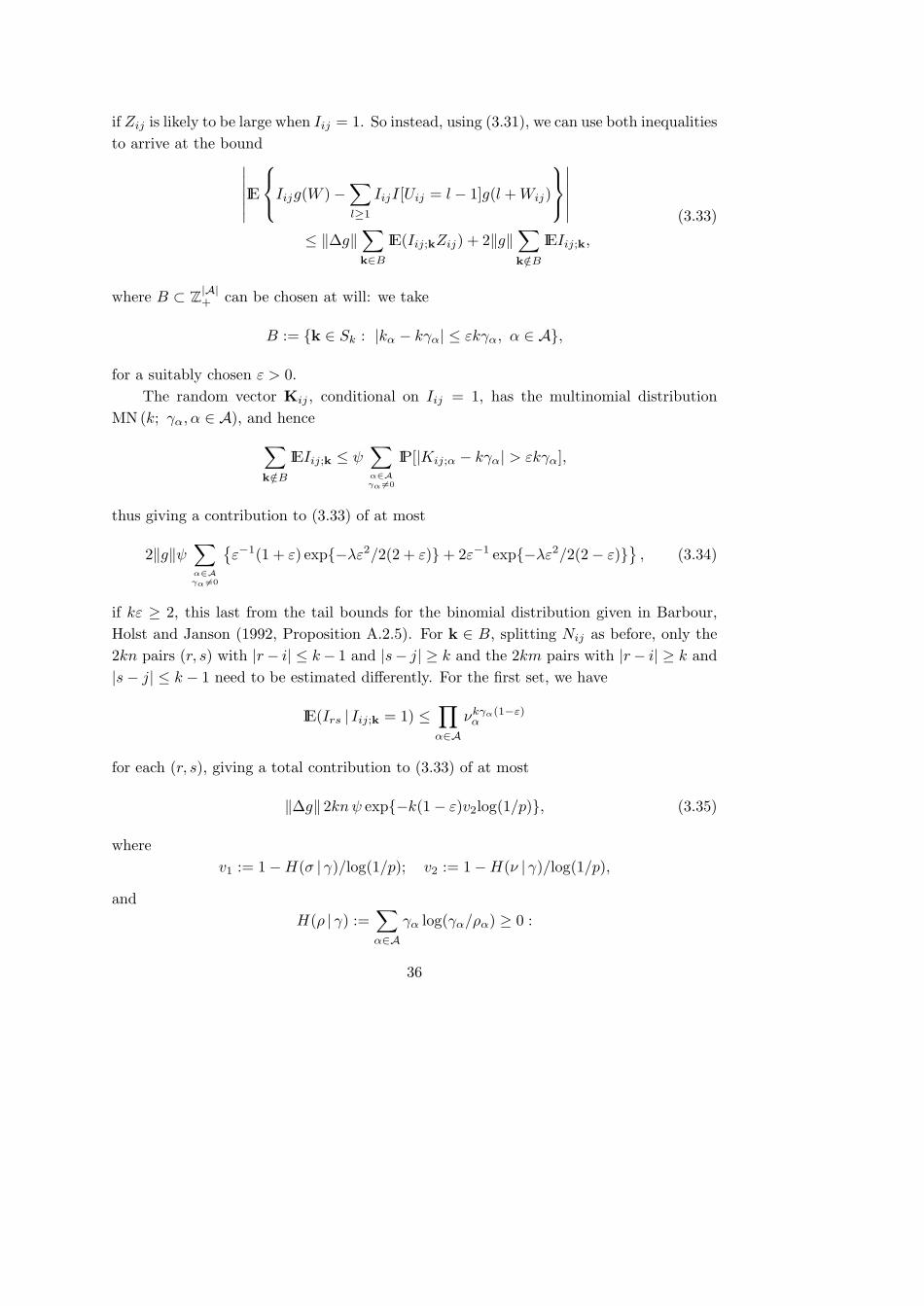
if Zij is likely to be large when Iij = 1. So instead, using (3.31), we can use both inequalitiesto arrive at the bound∣∣∣∣∣∣IE

Iijg(W )−∑l≥1

IijI[Uij = l − 1]g(l +Wij)

∣∣∣∣∣∣

≤ ‖∆g‖∑k∈B

IE(Iij;kZij) + 2‖g‖∑k/∈B

IEIij;k,

(3.33)

where B ⊂ 6 6 |A|+ can be chosen at will: we take

B := k ∈ Sk : |kα − kγα| ≤ εkγα, α ∈ A,

for a suitably chosen ε > 0.The random vector Kij , conditional on Iij = 1, has the multinomial distribution

MN (k; γα, α ∈ A), and hence∑k/∈B

IEIij;k ≤ ψ∑α∈Aγα 6=0

IP[|Kij;α − kγα| > εkγα],

thus giving a contribution to (3.33) of at most

2‖g‖ψ∑α∈Aγα 6=0

ε−1(1 + ε) exp−λε2/2(2 + ε)+ 2ε−1 exp−λε2/2(2− ε)

, (3.34)

if kε ≥ 2, this last from the tail bounds for the binomial distribution given in Barbour,Holst and Janson (1992, Proposition A.2.5). For k ∈ B, splitting Nij as before, only the2kn pairs (r, s) with |r− i| ≤ k− 1 and |s− j| ≥ k and the 2km pairs with |r− i| ≥ k and|s− j| ≤ k − 1 need to be estimated differently. For the first set, we have

IE(Irs | Iij;k = 1) ≤∏α∈A

νkγα(1−ε)α

for each (r, s), giving a total contribution to (3.33) of at most

‖∆g‖ 2knψ exp−k(1− ε)v2log(1/p), (3.35)

wherev1 := 1−H(σ | γ)/log(1/p); v2 := 1−H(ν | γ)/log(1/p),

andH(ρ | γ) :=

∑α∈A

γα log(γα/ρα) ≥ 0 :

36

the second set contributes at most

‖∆g‖ 2kmψ exp−k(1− ε)v1log(1/p) (3.36)

to (3.33). The sum of the three contributions (3.34)–(3.36) is then added over the (m−k+1)(n− k+ 1) possible pairs (i, j), and the improved bounds for ‖g‖ and ‖∆g‖ are applied.This yields alternative error estimates in place of (3.20):

dK (L(W ),CP (λ,µ)) ≤ 1(1− p)2 + λ−1

∆′1 + ∆2 + CK(p)mnψ1/2∆3, p ≤ 1/3;

dTV (L(W ),CP (λ,µ)) ≤ 1− p1− 5p

∆′1 + ∆2 + 2mnψ1/2∆3, p < 1/5,

(3.37)where

∆′1 := 2km exp−k(1− ε)v1log(1/p)+ n exp−k(1− ε)v2log(1/p)

+ 3(m+ n)pk + 2kγk+

;

∆3 :=∑α∈Aγα 6=0

ε−1(1 + ε) exp−kγαε2/2(2 + ε)+ 2ε−1 exp−kγαε2/2(2− ε)

,

(3.38)

∆2 is as in (3.21), and CK(p) := 23/2e((1− p)2 + λ−1)−1/2.In the circumstances illustrated in (3.23), provided that li < vi, i = 1, 2, a suitable

choice for ε is given by

ε = 1−max

√l1v1,

√l2v2

. (3.39)

This has the effect of replacing the exponents δ1 and δ2 in (3.29) by ε/(1− ε), and addingthe element involving ∆3; this alternative bound can then be used whenever kε ≥ 2.In asymptotic terms, it is now enough that l∗i < vi, i = 1, 2, which is a less restrictivecondition than (3.30), to allow the choice of

ε∗ = 1−max

√l∗1v1,

√l∗2v2

, (3.40)

for ε, in which case the overall error estimate is of order O(p−cn−δ) = O(IEWn−δ) forsome δ > 0; this once again converges to zero, as long as IEW only grows with n at mostas fast as a small power of n.

3.6 Markov chains.

Counting both success runs and occurrences of a word can be rephrased as particularcases of the more general problem of counting the number of visits W to a ‘rare’ set S1

37

in n steps of a recurrent Markov chain X. For success runs, as in Section 3.1, the statespace S can be taken to be 0, 1, . . . , k, by setting Xi = j if ξi = ξi−1 = · · · = ξi−j+1 andξi−j = 0, 1 ≤ j ≤ k − 1, and Xi = k otherwise; then, apart from edge effects, the numberof success runs of length k becomes the number of visits of X to S1 = k. For copies of asingle word A = a1a2 . . . ak of length k in the Markov model of Section 3.4, set Xi = j if

max(0, l : ξi−l+1, . . . , ξi = a1a2 . . . al) = j ∈ 1, 2, . . . , k,

and set Xi = (ξi, 0) otherwise; the number of copies of A is then the number of visits toS1 = k. When visits to S1 generally occur singly, a Poisson approximation to L(W )is appropriate (Barbour, Holst and Janson (1992, Section 8.5)), but it is more often thecase that there is a tendency for visits to occur in clumps, and then compound Poissonapproximation gives much sharper results.

This problem has been studied in some generality by Erhardsson (1999), exploiting theregenerative structure of a recurrent Markov chain to derive very pleasing approximationtheorems. The Markov chain X is assumed to be stationary and Harris recurrent on S,having a unique stationary distribution ν, and W =

∑ni=1 1Xi∈S1 counts the number of

visits to S1 ∈ S: define ψ := ν(S1). The approximating compound Poisson distributionCP (λ,µ) is defined in terms of regeneration cycles; λ is the expected number of cyclesin 1, 2, . . . , n which contain at least one visit to S1, and µ is the conditional distributionof the number of visits to S1 in a cycle, given that at least one occurs. In particular,if S1 is an atom — for example, a single state — then µ is geometric, and CP (λ,µ) is aPolya–Aeppli distribution. A formal definition of λ and µ is given in Erhardsson (1999,Definition 3.2).

The simplest theorem is obtained when regeneration is defined in terms of visits to anatom S0 such that ν(S0) > 0 and S0 ∩ S1 = ∅. In the example of success runs, the choiceS0 = 0 is appropriate; for the occurrence of a word, any singleton of the form (a, 0)could be used, or one could take S0 = ∪a∈A′(a, 0), for any collection A′ ⊂ A such thatπ(a, ·) is the same for all a ∈ A′. Let τS0 and τS1 denote the first times that X hits S0

and S1, τRS0the first time that the reversed chain hits S0. Then Erhardsson uses CPA 1A

combined with a coupling argument to prove that

dTV (L(W ),CP (λ,µ))

≤ 2HTV1 (λ,µ)nψ2

IEν|S1(τS0 + τRS0

) + ν−1(S0)IEν(τS0)

+ 2IPν [τS1 < τS0 ].(3.41)

Good bounds for HTV1 (λ,µ) are currently only known under either of Conditions

(2.18) and (2.20). In the examples of word counts and success runs, when Condition (2.20)holds, the results obtained for total variation approximation are nonetheless of the bestasymptotic order generally known. Erhardsson (1999) shows that (2.18) holds whenever

ν ess supx∈S1

IPx[τS1 < τS0 ] ≤ 3− 2ν ess infx∈S1

IPx[τS1 < τS0 ]−1,

38

and that thenλ(µ1 − 2µ2) ≥ nψ1− 4IPν|S1 [τS1 < τS0 ],

enabling HTV1 (λ,µ) to be effectively bounded using (2.19) in these circumstances. More

particularly, if S1 is an atom, as is the case in the examples of success runs and occur-rences of a word, then µj = (1 − p)pj−1 for j ≥ 1, where p = IPS1 [τS1 < τS0 ], and thusCondition (2.18) holds for p ≤ 1/2 with µ1 − 2µ2 = (1− p)(1− 2p), and the approximat-ing distribution is then a Polya–Aeppli distribution. However, the regenerative structureof such a Markov chain also lends itself well to proving good bounds for the quantityIP[W ≤ φλm1] in CPA 2A, so that it is to be expected that the better asymptotic ordernormally given by CPA 2A could be achieved here, too, when Condition (2.18) fails tohold.

Acknowledgement. ADB thanks the Department of Mathematics and Statistics atMonash University for their warm hospitality while part of this paper was being writ-ten.

References

[] Aldous, D.J. (1989). Probability approximations via the Poisson clumping heuristic.Springer, New York.

[] Arratia, R., Goldstein, L. and Gordon, L. (1989). Two moments suffice forPoisson approximations: the Chen–Stein method. Ann. Probab., 17, 9–25.

[] Arratia, R., Goldstein, L. and Gordon, L. (1990). Poisson approximation andthe Chen–Stein method. Stat. Sci., 5, 403–34.

[] Arratia, R., Gordon, L. and Waterman, M.S. (1990) The Erdos–Renyi law indistribution, for coin tossing and sequence matching. Ann. Statist. 18, 539–570.

[] Arratia, R., Martin, D., Reinert, G., and Waterman, M.S. (1996) Pois-son process approximation for sequence repeats and sequencing by hybridization.J. Comp. Biol , 3, 425–463.

[] Barbour, A.D. (1999) Topics in Poisson approximation. Handbook of Statistics, (toappear).

[] Barbour, A.D., Chen, L.H.Y. and Loh, W.–L. (1992). Compound Poissonapproximation for non–negative random variables via Stein’s method. Ann. Probab.20, 1843–66.

39

[] Barbour, A.D., Chryssaphinou, O., Roos, M. (1995). Compound Poisson Ap-proximation in Reliability Theory. IEEE Trans. Reliability 44, 398–402.

[] Barbour, A.D., Chryssaphinou, O., Roos, M. (1996). Compound Poisson ap-proximation in systems reliability. Naval Res. Logistics 43, 251–264.

[] Barbour, A.D., Chryssaphinou, O. and Vaggelatou, E. (2000) Applicationsof compound Poisson approximation. Statistical Distribution Theory and Inference.Eds. N. Balakrishnan, M.V. Koutras and C. Charalambides, CRC Press. (to appear).

[] Barbour, A.D. and Hall, P. (1984). On the rate of Poisson convergence. Math.Proc. Cam. Phil. Soc., 95, 473–80.

[] Barbour, A.D., Holst, L. and Janson, S. (1992). Poisson approximation. Ox-ford University Press.

[] Barbour, A.D. and Mansson, M. (1999) Compound Poisson approximation andthe clustering of random points. Adv. Appl. Probab. (to appear).

[] Barbour, A.D. and Utev, S. (1998). Solving the Stein Equation in compoundPoisson approximation. Adv. Appl. Probab. 30, 449–475.

[] Barbour, A.D. and Utev, S. (1999). Compound Poisson approximation in totalvariation. Stoch. Procs Applics 82, 89–125.

[] Barbour, A.D. and Xia, A. (1999a) Estimating Stein’s constants for compoundPoisson approximation. Bernoulli (to appear)

[] Barbour, A.D. and Xia, A. (1999b) Poisson perturbations. ESAIM: P&S 3, 131–150.

[] Barlow, R.E., Hunter, L.C. and Proschan, F. (1963) Optimum redundancywhen components are subject to two kinds of failure. J. Soc. Indust. Appl. Math. 11,64–73.

[] Le Cam, L. (1960). An approximation theorem for the Poisson binomial distribution.Pacific J. Math., 10, 1181–97.

[] Chao, M.T., Fu, J.C., and Koutras, M.V. (1995) A Survey of the Reliabil-ity Studies of Consecutive-k-Out-Of-n:F System and Related Systems. IEEE Trans.Reliability. 44, 120–127.

[] Chen, J. and Glaz, J. (1996) Two dimensional discrete scan statistics. Stat. Probab.Letters 31, 59–68.

[] Chen, R.W., Hwang, F.K., and Li, W.-C.W. (1993) Consecutive-2-out-of-n-:Fsystems with node and link failures. IEEE Trans. Reliability , 42, 497–502.

40

[] Chryssaphinou, O. and Papastavridis, S. (1988a) A limit theorem for the num-ber of non-overlapping occurrences of a pattern in a sequence of independent trials.J. Appl. Prob., 25, 428–431.

[] Chryssaphinou, O. and Papastavridis, S. (1988b) A limit theorem for the numberof overlapping appearances of a pattern in a sequence of independent trials. Prob.Theory Rel. Fields. 79, 129–143.

[] Chryssaphinou, O. and Papastavridis, S. (1990) Limit distribution for a consec-utive–k–out–of–n:F system. Adv. Appl. Prob., 22, 491–493.

[] Chryssaphinou, O., Papastavridis, S., and Vaggelatou, E. (1999) On thenumber of appearances of a word in a sequence of i.i.d. trials. Meth. Comp. Appl.Probab. 1, 329–348.

[] Chryssaphinou, O., Papastavridis, S., and Vaggelatou, E. (2000) Poisson Ap-proximation for the non–overlapping appearances of several words in Markov chains.Comb. Prob. Computing (to appear).

[] Chryssaphinou, O. and Vaggelatou, E. (1999a) Compound Poisson approxima-tion for the numbers of long increasing sequences. J. Appl. Probab. (to appear).

[] Chryssaphinou, O. and Vaggelatou, E. (1999b) Compound Poisson approxima-tion for multiple runs in a Markov chain. Ann. Inst. Statist. Math. (to appear).

[] Eichelsbacher, P. and Roos, M. (1999) Compound Poisson approximation fordissociated random variables via Stein’s method. Comb. Prob. Computing 8, 335–346.

[] Engle, R. (1995) ARCH. Oxford University Press.

[] Erhardsson, T. (1997) Compound Poisson approximation for Markov chains. Ph.D.Thesis, Royal Institute of Technology, Stockholm.

[] Erhardsson, T. (1999) Compound Poisson approximation for Markov chains usingStein’s method. Ann. Appl. Probab. 27, 565–596.

[] Fu, J.C. and Koutras, M.V. (1994) Poisson approximations for 2 dimensionalpatterns. Ann. Inst. Stat. Math. 46, 179–192.

[] Geske, M.X., Godbole, A.P., Schaffner, A.A., Skolnick, A.M., and Wall-

strom, G.L. (1995) Compound Poisson approximation for word patterns underMarkovian hypotheses. J. Appl. Prob. 32, 877–892.

[] Glaz, J. (1996) Discrete scan statistics with applications to minefield detection. InProc. Conf. SPIE, 2765, Orlando FL, 420–429.

41

[] Glaz, J. and Balakrishnan, N. (1999) Scan statistics and applications. Birk-hauser, Boston.

[] Glaz, J., Naus, J., Roos, M. and Wallenstein, S. (1994) Poisson approxima-tions for the distribution and moments of ordered m-spacings. J. Appl. Prob. 31,271–281.

[] Godbole, A. (1991) Poisson approximations for runs and patterns of rare events.Adv. Appl. Prob., 23, 851–865.

[] Godbole, A.P., Schaffner, A.A. (1993) Improved Poisson approximations forword patterns. Adv. Appl. Prob., 25, 334–347.

[] Goovaerts, M.J. and Dhaene, J. (1996) The compound Poisson approximationfor a portfolio of dependent risks. Insurance Math. Econ. 18, 81–85.

[] Huffer, F. and Lin, C.T. (1997) Approximating the distribution of the scan statis-tic using moments of the number of clumps. J. Amer. Stat. Soc. 92, 1466–1475.

[] Janson, S. (1990) Poisson approximation for large deviations. Rand. Struct. Alg. 1,221–229.

[] Janson, S. (1998) New versions of Suen’s correlation inequality. Rand. Struct. Alg.13, 467–483.

[] Koutras, M.V. (1997) Consecutive–k, r–out–of–n:DFM systems. Microelectron.Reliab. 37, 597–603.

[] Koutras, M.V., Papadopoulos, G.K., and Papastavridis, S.G. (1993) Reli-ability of 2-Dimensional Consecutive-k-out-of-n:F Systems. IEEE Trans. Reliability,44, 658-661.

[] Mansson, M. (1999). On compound Poisson approximation for sequence matching.Preprint.

[] Michel, R. (1988). An improved error bound for the compound Poisson approx-imation of a nearly homogeneous portfolio. ASTIN Bulletin, 17, 165–169.

[] von Mises, R. (1921) Das Problem der Iterationen. Z. Angew. Math. Mech., 1,298–307.

[] Neuhauser, C. (1994) A Poisson approximation for sequence comparisons with in-sertions and deletions. Ann. Statist. 22, 1603–29.

[] Neuhauser, C. (1996) A phase transition for the distribution of matching blocks.Comb. Prob. Computing 5, 139–59.

42

[] Novak, S. (1994) Poisson approximation for the number of long match patterns inrandom sequences. Theor. Prob. Appl. 39, 593–603.

[] Pittel, B.G. (1981) Limiting behavior of a process of runs. Ann. Prob. 9, 119–129.

[] Preston, C.J. (1973) Generalized Gibbs states and Markov random fields. Adv.Appl. Probab. 5, 242–261.

[] Reinert, G., and Schbath, S. (1998) Compound Poisson and Poisson processapproximations for occurrences of multiple words in Markov chains. J. Comp. Biol.,5, 223–253.

[] Revesz, P. (1983) Three problems on the lengths of increasing runs.Stoch. Proc.Appl., 15, 169–179.

[] Roos, M. (1993) Stein–Chen method for compound Poisson approximation. Ph.D.Thesis, Universitat Zurich.

[] Roos, M. (1994). Stein’s method for compound Poisson approximation: the localapproach. Ann. Appl. Prob., 4, 1177–1187.

[] Ross, S. (1979) Multivalued state component systems. Ann. Probab. 7, 379–383.

[] Salvia, A.A., and Lasher, W.C. (1990). 2-Dimensional Consecutive- k-Out-Of-n:F Models. IEEE Trans. Reliability 39, 382–385.

[] Satoh, N., Sasaki, M., Yuge, T. and Yanasi, S. (1993) Reliability of three statedevice systems. IEEE Trans. Reliability 42, 470–477.

[] Schbath, S. (1995) Compound Poisson approximation of word counts in DNA se-quences. ESAIM: P&S , 1, 1–16.

[] Suen, W.C.S. (1990) A correlation inequality and a Poisson limit theorem for non-overlapping balanced subgraphs of a random graph. Rand. Struct. Alg., 1, 231–242.

[] Waterman, M.S. (1995) Introduction to computational Biology. Chapman and Hall,London.

[] Wolfowitz, J. (1944) Asymptotic distribution of runs up and down. Ann. Math.Stat. 15, 163–172.

43