lable at ScienceDirect

Environmental Modelling & Software 26 (2011) 804e816

Contents lists avai

Environmental Modelling & Software

journal homepage: www.elsevier .com/locate/envsoft

Component-based development and sensitivity analyses of an air pollutantdry deposition model

Satoshi Hirabayashi a, Charles N. Kroll b,*, David J. Nowak c

a The Davey Tree Expert Company, 5 Moon Library, SUNY College of Environmental Science and Forestry, Syracuse, New York 13210, United Statesb Environmental Resources Engineering, SUNY College of Environmental Science and Forestry, 1 Forestry Drive, 402 Baker Laboratory, Syracuse, New York 13210, United StatescUSDA Forest Service, Northeastern Research Station, 5 Moon Library, SUNY College of Environmental Science and Forestry, Syracuse, New York 13210, United States

a r t i c l e i n f o

Article history:Received 30 August 2009Received in revised form22 November 2010Accepted 28 November 2010Available online 19 January 2011

Keywords:Air pollutantDry depositionComponent-based modelUFORESensitivity analysis

* Corresponding author. Tel.: þ1 315 470 6699; faxE-mail addresses: satoshi.hirabayashi@davey.com

edu (C.N. Kroll), dnowak@fs.fed.us (D.J. Nowak).

1364-8152/$ e see front matter � 2010 Elsevier Ltd.doi:10.1016/j.envsoft.2010.11.007

a b s t r a c t

The Urban Forest Effects-Deposition model (UFORE-D) was developed with a component-based modelingapproach. Functions of the model were separated into components that are responsible for user interface,data input/output, and core model functions. Taking advantage of the component-based approach, threeUFORE-Dapplicationswere developed: a base application toestimatedry deposition at anhourly time step,and two sensitivity analyses based onMonte Carlo simulations with a Latin hypercube sampling (LHS-MC)andaMorris one-at-a-time (MOAT) sensitivity test.With thebase application, drydeposition of CO,NO2,O3,PM10, and SO2 in the city of Baltimorewas estimated for 2005. The sensitivity applicationswere performedto examine UFORE-D model parameter sensitivity. In general, dry deposition velocity was sensitive totemperature and leaf area index (LAI). Temperature had a non-linear effect on all pollutants, while LAI wasimportant to NO2 deposition with a nearly linear effect. PAR and wind speed had limited effects on drydeposition of all pollutants; dry depositionwas affected by PAR and wind speed only up to their thresholdvalues. The component-based approach allows for seamless integration of new model elements, andprovides model developers with a platform to easily interchange model components.

� 2010 Elsevier Ltd. All rights reserved.

Software availability

Name of software: UFORE-DDeveloper: Satoshi Hirabayashi, The Davey Tree Expert Company,

5 Moon Library, SUNY-ESF, 1 Forestry Drive, Syracuse,NY 13210

Tel.: þ1 315 448 3201Fax: þ1 315 448 3216E-mail: satoshi.hirabayashi@davey.comFirst available: 2011 (integrated with i-Tree Eco)Hardware required: PC running Windows XP or laterSoftware required: NoneProgram language: Visual BasicCost: Will be freely downloadable from http://www.itreetools.org/

in 2011.

1. Introduction

Environmental computer models are traditionally developed asclosed monolithic systems (Bian, 2000; He et al., 2002). Individual

: þ1 315 470 5968.(S. Hirabayashi), cnkroll@esf.

All rights reserved.

research groups develop models suited for their purposes withintheir development platforms or modeling frameworks. Suchmodels typically allow users to access themodel only through inputand output data, with no controls over the core model elements.When the models are released into the public domain these limi-tations become an issue for users who wish to make changes to themodel. New applications are often built upon existing publicdomain models, or existing models are integrated into largermodeling frameworks. Such tasks often require users to learn andmodify the model source code, which can be hard due to differ-ences in programming languages, software architecture, or mod-eling frameworks. Data for the models are traditionally stored ina text file; however, new data storage schemes have becomepopular for improved handling of large amounts of data. To intro-duce new data formats into existing models, the model typicallymust be modified at the source code level. The lack of reusabilityand flexibility in the closed monolithic models create duplicatedefforts, resulting in wasted time and energy.

The Urban Forest Effects-Deposition model (UFORE-D) is a publicdomain computer program widely used to quantify dry deposition(i.e. pollution removal during non-precipitation periods) to forestcanopies in urban areas in North America (Nowak et al., 1998, 2000,2006; Nowak and Crane, 2000; Deutsch et al., 2005; Currie and Bass,2008). Because UFORE-D is a closed system, implemented as a large

Fig. 1. Component structure of UFORE-D applications.

S. Hirabayashi et al. / Environmental Modelling & Software 26 (2011) 804e816 805

code written in SAS (Statistical Analysis Software), it is difficult forusers to reuse UFORE-D for new applications. Furthermore, since thedata format of UFORE-D are limited to text or SAS binary formats,employing different data formats such as a relational databaserequires modifications in the source codes.

These modeling problems may be overcome by employingComponent-Based Software Engineering (CBSE) concepts. CBSE isan emerging paradigm in software development and is seen asa major new direction in the post object-oriented approach era(Bian, 2000). CBSE breaks the executable model code into separatepieces or components. A component comes packaged as a binarycode ready to perform certain tasks for the entire model. Compo-nents connect to each other at run time to form a complete model.CBSE requires a binary architecture standard to regulate howcomponents interact at run time (Argent, 2004). A widely usedstandard is the Component Object Model (COM) that Microsoftintroduced for the Windows platform (Chappell, 1996). The use ofcomponents allows component transplanting, or the so-called ‘plugand play’ approach. While maintaining model integrity, a compo-nent of the model can be easily replaced with a new component.For instance, if data input/output functions are developed ascomponents, a format change of the data requires replacing onlythese components. A component that performs model core func-tionality can be easily reused in other model applications. Evenmodels developed in different frameworks can be readily merged ifthe frameworks comply with a CBSE standard such as COM. Thus,component-based approaches can drastically enhance the reus-ability and interoperability of environmental computer models.

In this study, development of UFORE-D with COM technology isreported. The developed components can collectively perform thesame dry deposition modeling functions the original UFORE-Doffers. As a case study, the dry deposition of five criteria airpollutants (CAPs), carbon monoxide (CO), nitrogen dioxide (NO2),ozone (O3), particulate matter less than 10 microns (PM10), andsulfur dioxide (SO2), are quantified in Baltimore, MD in 2005.

Inenvironmentalmodelbuildingprocesses, examiningsensitivityof a model to changes in its parameters and inputs is an importantmodel evaluation exercise. Sensitivity analyses allow one to gainknowledge of how the modeled system functions and to identify

parameters of the model whose values need to be specified moreaccurately (Barnsley, 2007). Historically, sensitivity analyses havebeen performed in the development of environmental models(LiepmannandStephanopoulos,1985;MacKerronandWaister,1985;Caton et al., 1999; Hermann et al., 2002; Weiler, 2005; Pohlert et al.,2007) including air pollutant models (Anfossi et al., 1996; Smithet al., 2000; Simpson et al., 2003; Wu et al., 2003; MacDougallet al., 2005; Ziehn and Tomlin, 2008; Mészáros et al., 2009).A variety of sensitivity analysis techniques have been proposed andreviewed in the literature (Hamby, 1994; Campolongo and Saltelli,1997; Saltelli et al., 2000; Ravalico et al., 2005; Norton, 2008).

In the current study, two sensitivity analysis applications ofCOM-based UFORE-D are performed by reusing developed COMcomponents. Development of these two applications exemplifiesthe components’ transplantability and reusability. Through thisexercise, the UFORE-D model is run for a wide range of modelparameters that are representative of many vegetation andweatherconditions observed throughout the United States, and theparameters the model is most sensitive to are identified.

2. Component and application design

Information systems are conceptually designed around threelayers: presentation, logic, and data management (Alonso et al.,2004). The presentation layer provides a user interface and anoverall control of applications. The logic layer controls a system’sfunctionality by performing detailed processing. The datamanagement layer handles data access and management. Thisarchitecture was adopted in this study to efficiently separatefunctionalities of UFORE-D into components that are responsiblefor specific tasks.

The developed components in the three layers are illustrated inFig. 1. The five components in the data management layer, the DryDeposition component in the logic layer, and the Base component inthe presentation layer are assembled to perform the same functionsas the original UFORE-D. Two more applications, Monte Carlo withLatin hypercube sampling (LHS-MC) and Morris one-at-a-time(MOAT) sensitivity analyses, which can perform a global sensitivityanalysis of UFORE-D, are also developed. For these applications,

S. Hirabayashi et al. / Environmental Modelling & Software 26 (2011) 804e816806

components in the logic and data management layers are all reused;only components in the presentation layer are replaced.

COM components are generally developedwithMicrosoft VisualStudio, an integrated development environment (IDE) that includesfeatures for editing, compiling, linking, deploying, and debuggingsoftware. Visual Basic (VB) 6.0 is used in this study. Components inthe presentation layer are compiled into standard executables,while components in the logic and data management layers arecompiled into ActiveX dynamic link libraries (DLLs). The standardexecutables are COM clients that get a pointer to a COM server anduse its services by calling themethods of its interfaces. The DLLs areCOM server components that provide services to clients in the formof COM interface implementations (MSDN, 2009). Design andfunctions of each component are explained in the next sections.

2.1. Data read/write components

UFORE-D takes a variety of data as its input and quantifies drydeposition of air pollutants in a city. Input data includes locationrelated information, urban forest information, hourly meteorologyand air pollutant concentration data. The location informationincludes time zone, latitude, longitude, and leaf-on and leaf-off dates.Urban forest characteristics include the maximum leaf area index(LAI) during the leaf-on season, tree coverage, and evergreen canopypercentages that can be used to approximate the minimum LAIduring the leaf-off season. LAI is defined as the total area of leaves(one-sided) per unit ground surface area projected on the horizontaldatum (NASA, 2009). UFORE-D outputs hourly results as well assummaries for longer periods. These data are stored in either text orSAS binary files in the original UFORE-D, while all data are stored inMicrosoft Access databases in this study.With the relational databasemanagement functions and the structured query language (SQL) thatAccess offers, data extraction and summarization needed in theapplications of this study can be effectively and efficiently achieved.

Using the city name and code as keys, the Location Database(DB) Reader and the Urban Forest DB Reader components issue anSQL command to the corresponding Access database to extractrecords for a specific city. Using SQL commands, the MeteorologyDB Reader and the Air Pollutant DB Reader components offerflexibility for extracting records from the corresponding Accessdatabases. Hourly records extracted can be specified for a certainperiod of hours in either a specific month or a period of Julian dates.In addition, these components calculate statistics (mean, minimum,maximum, and standard deviation) of data fields in the extractedrecords. Similarly, the Output DB Writer component providesseveral methods to output results, including hourly, daily, monthly,leaf-on and leaf-off season results, and annual summaries, into thecorresponding Access databases.

2.2. Dry deposition component

The Dry Deposition component performs UFORE-D’s core func-tion, inwhich hourly dry deposition of CO, NO2, O3, PM10 and SO2 isestimatedwith hourlymeteorological and pollutantmeasurements,location information, and urban forest parameters. A brief modeldescription is included below. Readers are referred to Hirabayashiet al. (2010) for a more complete description of the model.

Pollutant flux, F (gm�2 s�1), is estimated as a product of the drydeposition velocity, Vd (m s�1), and the air pollutant concentration,C (gm�3):

F ¼ Vd$C (1)

Vd is estimated as the inverse of the sum of resistances to pollutanttransport (Baldocchi et al., 1987):

Vd ¼ ðRa þ Rb þ RcÞ�1 (2)

where Ra represents air movement resistance in the crown space(aerodynamic resistance), Rb represents transfer resistance throughthe boundary layer immediately adjacent to canopy surfaces(quasi-laminar boundary layer resistance), and Rc represents thechemical and biological absorption capacity of the canopy surfaces(canopy resistance). Ra is calculated as (Killus et al., 1984):

Ra ¼ uðzÞu2�

(3)

where u(z) is the meanwind speed at height z, and u� is the frictionvelocity calculated as a function of u(z), roughness length,displacement length, and temperature, depending upon atmo-spheric stability (Venkatram, 1980; Dyer and Bradley, 1982; Killuset al., 1984; van Ulden and Holtslag, 1985; US EPA, 1995). Rb iscalculated as (Pederson et al., 1995):

Rb ¼ 2ðScÞ2=3ðPrÞ�2=3ðku*Þ�1 (4)

where Sc is the Schmidt number, Pr is the Prandtl number, and k isthe von Karman constant (¼0.41).

Hourly Rc for NO2, O3, and SO2 is calculated based on a hybrid ofthe big-leaf and multilayer canopy deposition models (Baldocchiet al., 1987; Baldocchi, 1988; Norman, 1980). Rc depends on fourcomponents: stomatal resistance (rs), mesophyll resistance (rm),cuticular resistance (rt), and soil resistance (rsoil):

1Rc

¼ 1rs þ rm

þ 1rtþ 1rsoil

(5)

rm was set to 10 sm�1 for O3 (Hosker and Lindberg, 1982), and0 sm�1 for SO2 (Wesely, 1989). rm for NO2 was set to 100 sm�1

(Hosker and Lindberg, 1982) to account for the difference betweenwater vapor and NO2 transport within mesophyll air spaces, and toensure the Vd calculated was in the typical range reported by Lovett(1994). rt was set to 20,000 sm�1 for NO2 based upon Wesely(1989) assuming mixed forest in midsummer, and calculated as10,000 sm�1 for O3, and 8000 sm�1 for SO2 to account for thetypical variation in rt exhibited among the pollutants (Taylor et al.,1988; Lovett, 1994). rsoil was set to 2000 sm�1 (Meyers andBaldocchi, 1993). Derivation of stomatal conductance, gs, theinverse of rs, is based on its link to leaf photosynthesis. gs can beexpressed as a function of net leaf photosynthesis (A), leaf surfacerelative humidity (rh), and the leaf surface CO2 concentration (Cs)(Collatz et al., 1991; Leuning, 1990; Baldocchi, 1994):

gs ¼ mArhCs

þ b0 (6)

The coefficient m is a dimensionless slope (¼10) and b0 is the zerointercept when A is equal to or less than zero (¼0.02 molm�2 s�1).A can be expressed as (Farquhar et al., 1980; Harley et al., 1992):

A ¼ Vc � 0:5Vo � Rd (7)

Vc and Vo are the carboxylation and oxygenation rate of CO2exchange between the leaf and the atmosphere, respectively. Rd isthe dark respiration rate of the CO2 exchange. A is a function of PAR,temperature, relative humidity, and wind speed. An analyticalsolution of A is described in detail in Baldocchi (1994). While earlierstudies by Farquhar et al. (1980), Norman (1980), Leuning (1990),Collatz et al. (1991), and Harley et al. (1992) related the photo-synthesis (A) by C3 grasses to gs, later studies by Harley andBaldocchi (1995), Baldocchi and Harley (1995), Wilson et al.(2001), and Baldocchi and Wilson (2001) parameterized themodel for C3 trees. UFORE-D was parameterized for trees based onthese later studies. Cs can be expressed as (Baldocchi, 1994):

Table 1Summary statistics of the UFORE-D input parameters for LHC-MC analysis.

Parameter Minimum Mean Maximum SD

LAI 2.5 5.8 10 1.7PAR (Wm�2) 38.6 296.8 503.8 132.2Pressure (hPa) 984.6 1011.4 1037.1 8.1Relative humidity (%) 15.6 53.2 100.0 18.4Temperature (�C) �7.8 16.5 34.5 10.7Wind speed (m s�1) 0.5 4.1 11.6 2.3

Table 2Annual estimates of air pollution removal by total tree canopy cover and per unittree canopy cover in Baltimore in 2005.

Air pollutant Total pollution removal(t)

Pollution removal perunit tree cover (gm�2)

Total Range Total Range

CO 7 na 0.2 naNO2 61 23e81 1.4 0.5e1.9O3 199 44e275 4.7 1.1e6.4PM10 136 53e212 3.2 1.2e5.0SO2 44 17e76 1.0 0.4e1.8

Total 447 137e645 10.5 3.2e15.1

S. Hirabayashi et al. / Environmental Modelling & Software 26 (2011) 804e816 807

Cs ¼ Ca � Agb

(8)

Ca is atmosphere’s CO2 concentration (set to the global annualmean of 380 ppm in 2005 (NOAA, 2010)). Note that the CO2concentration in the atmosphere is increasing continuously (NOAA,2010) and urban areas tend to have higher CO2 concentrations dueto human activities (Vitousek et al., 1997; Pataki et al., 2003). HigherCO2 concentrations may decrease gs, which leads to a decrease inthe air pollutant flux due to the dry deposition (Baldocchi, 1994;Wu et al., 2003). gb is conductance across the laminar boundarylayer of a leaf, and a reciprocal of the sum of Ra and Rb for CO2exchange.

To represent rs for the canopy level from rs for the individual leaflevel, Norman’s (1980) canopy radiation transfer/interceptionmodel is employed. In this approach the canopy is divided into Nlayers of equal leaf area index increments (DLAI) and each canopylayer is divided into two classes of leaves: sunlit and shaded. In thejth layer, stomatal conductances calculated separately for sunlit andshaded leaves (gs,sun,j and gs,shade,j, respectively) and combinedaccording to the fraction of sunlit and shaded leaf area indices(LAIsun,j and LAIshade,j, respectively) provide gs,j. The summation ofgs,j for the N layers provides the gs for the entire canopy.

0 1 2 3 4 5 6 7 8 9 10 11 12 13 14 15 16 17 18 19 20 21 22 23

0.0

0.2

0.4

0.6

0.8

V d(c

m s

-1)

a NO2

Hour

0 1 2 3 4 5 6 7 8 9 10 11 12 13 14 15 16 17 18 19 20 21 22 23

Hour

0.0

0.2

0.4

0.6

0.8

V d(c

m s

-1)

c SO2

Fig. 2. Hourly estimates of Vd for (a) NO2, (b) O3

gs ¼XNj¼1

gs;j ¼XNj¼1

�gs;sun;jLAIsun;j þ gs;shade;jLAIshade;j

�(9)

Derivation of sunlit and shaded components of LAI in each layeris based on Norman (1980).

LAIsun;j ¼�TB;j � TB;jþ1

�2cos q (10)

LAIshade;j ¼ DLAI� LAIsun;j (11)

TB;j ¼ exp�� LAIj2cos q

�(12)

TB,j represents the direct solar beam transmittance below layer j.LAIj is LAI below layer j. q is solar zenith angle.

To calculate gs,sun,j and gs,shade,j, PAR components on sunlit andshaded leaves in the jth layer (PARsun,j and PARshade,j, respectively)are used for the derivation of A in Eq. (6). PAR component iscalculated based on an assumption that shaded leaves receive onlydiffused solar radiation and sunlit leaves receive both direct and

0 1 2 3 4 5 6 7 8 9 10 11 12 13 14 15 16 17 18 19 20 21 22 23

0.0

0.2

0.4

0.6

0.8

V d(c

m s

-1)

b O3

Hour

, and (c) SO2 during leaf-on season in 2005.

Fig. 3. Scatterplots of Vd for NO2 and input parameters obtained from the LHS-MC sensitivity analysis.

S. Hirabayashi et al. / Environmental Modelling & Software 26 (2011) 804e816808

diffused solar radiation. Norman (1980, 1982) and Baldocchi et al.(1987) describe these processes and solutions in detail. In thisstudy, the scaling factor (Sj) was added to their functions to scalediffused PAR through the canopy layers.

PARshade;j ¼PARdiff exp��0:5LAI0:7

�Sj

þ 0:07PARdir

�1:1� 0:1

�LAIj �

DLAI2

�

expð�cos qÞ (13)

PARsun;j ¼ PARdircos acos q

þ PARshade;j (14)

PARdiff, PARdir are the flux density of diffuse and direct PAR abovethe canopy, respectively. LAI is leaf area index for the entire canopy,and a is mean angle between leaves and the sun (¼60�).

The divisions of solar irradiance into direct and diffuse compo-nents as well as into PAR and near-infrared components are basedon the method described in Weiss and Norman (1985). PAR iscalculated as 46 percent of total solar irradiance (Norman, 1982;Monteith and Unsworth, 1990) that is calculated based on theNational Renewable Energy Laboratory Meteorological/Statistical

Table 3Pearson product moment correlation coefficient (PMCC) between Vd and eachparameter.

Air pollutant Parameters

LAI PAR Pressure Relative humidity Temperature Wind speed

NO2 0.60a 0.27a 0.001 0.45a 0.29a 0.34a

O3 0.31a 0.33a �0.004 0.54a 0.35a 0.40a

SO2 0.27a 0.33a �0.004 0.56a 0.36a 0.38a

a Significantly different than zero at a 5% level.

Solar Radiation Model (METSTAT) with inputs from the meteoro-logical data set (Maxwell, 1998).

As removals of CO and PM10 by vegetation are not directly relatedto transpiration, Rc for COwas set to a constant for the leaf-on season(50,000 sm�1) and the leaf-off season (1,000,000 sm�1) based ondata fromBidwell and Fraser (1972). For PM10, themediandepositionvelocity (Lovett,1994) was set to 0.0064 m s�1 based on a 50-percentresuspension rate of particles back to the atmosphere (Zinke, 1967).The base Vd was adjusted according to actual LAI and a surface-areaindex for bark of 1.7 (m2 of bark per m2 of ground surface covered bythe tree crown) (Whittaker andWoodwell, 1967).

2.3. Base component

A single run of the original UFORE-D estimates dry deposition fora single air pollutant on an hourly basis and creates a variety ofsummaryoutput tables. Thebase component implementsexactly thesame functions and repeats it five times to process the five airpollutants in a single run. Annual summaries created include total airpollutant removal by dry deposition in the study area, total airpollutant removalperunit tree coverarea, and rangesof thesevalues.Monthly summaries include total air pollutant removal by drydeposition for eachmonth, which shows seasonal variation of urbanforest effects on air quality. Daily summaries show daily air pollutionremoval by the entire study area and per unit tree cover area in leaf-on and leaf-off seasons.

2.4. Monte Carlo with Latin hypercube sampling (LHS-MC)component

In the Monte Carlo (MC) analysis, a large number of parametersets are generated according to the probability density functions of

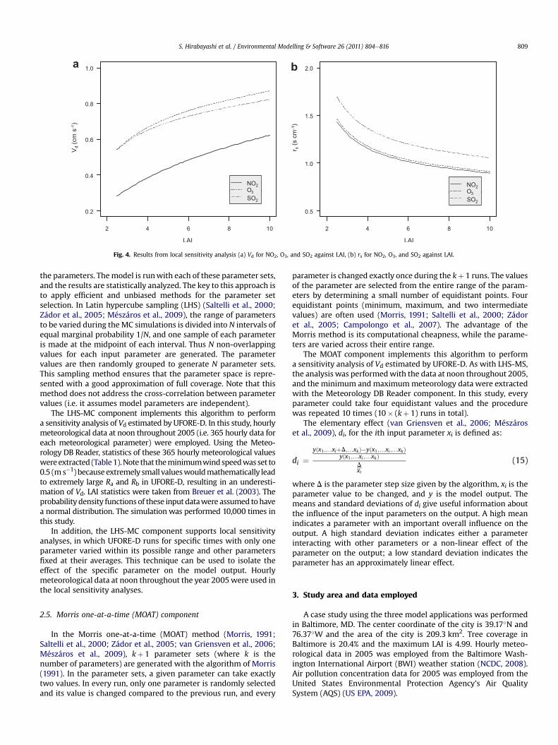
Fig. 4. Results from local sensitivity analysis (a) Vd for NO2, O3, and SO2 against LAI, (b) rs for NO2, O3, and SO2 against LAI.

S. Hirabayashi et al. / Environmental Modelling & Software 26 (2011) 804e816 809

the parameters. Themodel is runwith each of these parameter sets,and the results are statistically analyzed. The key to this approach isto apply efficient and unbiased methods for the parameter setselection. In Latin hypercube sampling (LHS) (Saltelli et al., 2000;Zádor et al., 2005; Mészáros et al., 2009), the range of parametersto be varied during the MC simulations is divided into N intervals ofequal marginal probability 1/N, and one sample of each parameteris made at the midpoint of each interval. Thus N non-overlappingvalues for each input parameter are generated. The parametervalues are then randomly grouped to generate N parameter sets.This sampling method ensures that the parameter space is repre-sented with a good approximation of full coverage. Note that thismethod does not address the cross-correlation between parametervalues (i.e. it assumes model parameters are independent).

The LHS-MC component implements this algorithm to performa sensitivity analysis of Vd estimated by UFORE-D. In this study, hourlymeteorological data at noon throughout 2005 (i.e. 365 hourly data foreach meteorological parameter) were employed. Using the Meteo-rology DB Reader, statistics of these 365 hourly meteorological valueswereextracted (Table1).Note that theminimumwindspeedwas set to0.5 (m s�1) because extremely small valueswouldmathematically leadto extremely large Ra and Rb in UFORE-D, resulting in an underesti-mation of Vd. LAI statistics were taken from Breuer et al. (2003). Theprobability density functions of these input datawere assumed tohavea normal distribution. The simulation was performed 10,000 times inthis study.

In addition, the LHS-MC component supports local sensitivityanalyses, in which UFORE-D runs for specific times with only oneparameter varied within its possible range and other parametersfixed at their averages. This technique can be used to isolate theeffect of the specific parameter on the model output. Hourlymeteorological data at noon throughout the year 2005were used inthe local sensitivity analyses.

2.5. Morris one-at-a-time (MOAT) component

In the Morris one-at-a-time (MOAT) method (Morris, 1991;Saltelli et al., 2000; Zádor et al., 2005; van Griensven et al., 2006;Mészáros et al., 2009), kþ 1 parameter sets (where k is thenumber of parameters) are generated with the algorithm of Morris(1991). In the parameter sets, a given parameter can take exactlytwo values. In every run, only one parameter is randomly selectedand its value is changed compared to the previous run, and every

parameter is changed exactly once during the kþ 1 runs. The valuesof the parameter are selected from the entire range of the param-eters by determining a small number of equidistant points. Fourequidistant points (minimum, maximum, and two intermediatevalues) are often used (Morris, 1991; Saltelli et al., 2000; Zádoret al., 2005; Campolongo et al., 2007). The advantage of theMorris method is its computational cheapness, while the parame-ters are varied across their entire range.

The MOAT component implements this algorithm to performa sensitivity analysis of Vd estimated by UFORE-D. As with LHS-MS,the analysis was performedwith the data at noon throughout 2005,and the minimum and maximummeteorology data were extractedwith the Meteorology DB Reader component. In this study, everyparameter could take four equidistant values and the procedurewas repeated 10 times (10� (kþ 1) runs in total).

The elementary effect (van Griensven et al., 2006; Mészároset al., 2009), di, for the ith input parameter xi is defined as:

di ¼yðx1;.xiþD;.xkÞ�yðx1 ;.xi;.xkÞ

yðx1 ;.xi;.xkÞDxi

(15)

where D is the parameter step size given by the algorithm, xi is theparameter value to be changed, and y is the model output. Themeans and standard deviations of di give useful information aboutthe influence of the input parameters on the output. A high meanindicates a parameter with an important overall influence on theoutput. A high standard deviation indicates either a parameterinteracting with other parameters or a non-linear effect of theparameter on the output; a low standard deviation indicates theparameter has an approximately linear effect.

3. Study area and data employed

A case study using the three model applications was performedin Baltimore, MD. The center coordinate of the city is 39.17�N and76.37�W and the area of the city is 209.3 km2. Tree coverage inBaltimore is 20.4% and the maximum LAI is 4.99. Hourly meteo-rological data in 2005 was employed from the Baltimore Wash-ington International Airport (BWI) weather station (NCDC, 2008).Air pollution concentration data for 2005 was employed from theUnited States Environmental Protection Agency’s Air QualitySystem (AQS) (US EPA, 2009).

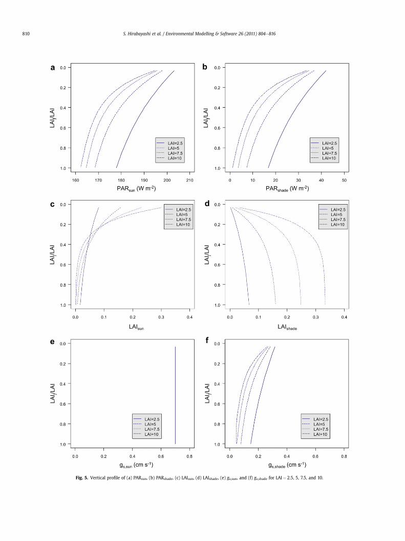
Fig. 5. Vertical profile of (a) PARsun, (b) PARshade, (c) LAIsun, (d) LAIshade, (e) gs,sun, and (f) gs,shade for LAI¼ 2.5, 5, 7.5, and 10.

S. Hirabayashi et al. / Environmental Modelling & Software 26 (2011) 804e816810

Fig. 6. Results from local sensitivity analysis (a) Vd against PAR, (b) Vd against relative humidity, and (c) Vd against temperature, and scatterplot obtained from LHS-MC for NO2 (d) Raagainst temperature, (e) Rc against temperature, and (f) resistances against wind speed.

S. Hirabayashi et al. / Environmental Modelling & Software 26 (2011) 804e816 811

4. Results and discussions

4.1. Air pollutant removal

Results obtained from the base application are presented in thissection. Table 2 presents annual removal statistics for 2005. Totalestimatedpollution removal by trees in the studyareawas447metrictonswithO3 (199 t) removed themost andCO (7 t) removed the least.Pollutant removal per unit tree cover area ranged from 0.2 gm�2 forCO to4.7 gm�2 forO3. Total pollutant removalperunit tree coverareawas 10.5 gm�2 for all five pollutants. These results are comparable tothose estimated by Nowak et al. (2006), in which the total pollutantremoval by treeswas 477metric tons and total pollutant removal perunit tree cover was 12.1 gm�2 for 1994 in Baltimore.

Vd during daytime in the leaf-on seasons for NO2 typicallyranges from 0.1 to 0.5 cm s�1 (Lovett, 1994). Daytime Vd for O3 inthe literature normally ranges from 0.3 to 1 cm s�1 and averagesaround 0.7 cm s�1 (Greenhut, 1983; Colbeck and Harrison, 1985;Davidson and Wu, 1990). Average daytime leaf-on Vd for SO2 forforests and trees in the literature typically ranges from 0.2 to2 cm s�1 and averages around 1.0 cm s�1 (Garland and Branson,1977; McMahon and Denison, 1979; Fowler and Cape, 1983;Lovett and Lindberg, 1984; Fowler, 1985; Lorenz and Murphy,1985; Murphy and Sigmon, 1990). Daytime deposition velocitiesestimated for the leaf-on season showed good agreements withthese values (Fig. 2).

4.2. LHS-MC analysis

The LHS-MC analysis provides a good estimate of the attainableminimum and maximum values of the model outputs (Zádor et al.,

2005; Mészáros et al., 2009), while the input parameters changeacross their possible ranges. This comprehensive approach is themain advantage of this method. One weakness of the method isthat it treats the parameters as independent variables, despite thefact that many inputs are highly correlated. For example, relativehumidity, temperature, and solar radiation are all highly correlatedand have a strong diurnal cycle. However, a wide range oftemperature can occur for a given relative humidity and vice versa,and this analysis covers the whole range of realistic values ofmeteorological parameters in the specific period. Nevertheless, asthis sensitivity test is simple and realistic it has been used in variousmodel developments.

A scatterplot between model parameter values and modeloutput is one of the most intuitive and straightforward techniquesto provide a qualitative measure of sensitivity (Saltelli et al., 2000).It may reveal relationships between model inputs and outputs,such as non-linear relationships and thresholds (Helton, 1993).Pearson product moment correlation coefficient (PMCC) is anothersimple measure of sensitivity, which is a measure of the linearrelationship between input and output values (Saltelli et al., 2000).Here PMCC is employed to explore the strength of the linear rela-tionship between input and output values.

Since UFORE-D calculates CO and PM10 removals based onconstants Rc and Vd, respectively, the results for these pollutantsare less affected by meteorological and vegetation parameters.Thus, the analysis presented here is limited to NO2, O3, and SO2.The input parameters analyzed are LAI, PAR, pressure, relativehumidity, temperature, and wind speed. Fig. 3 presents scatter-plots of Vd for NO2 and the given input parameter, and Table 3presents PMCC between Vd and the parameters calculated forNO2, O3, and SO2.

Fig. 7. Results from local sensitivity analysis (a) Vd against rm, (b) Vd against rt, and (c) Vd against rsoil.

S. Hirabayashi et al. / Environmental Modelling & Software 26 (2011) 804e816812

LAI is a major parameter governing the computations of rm, rt,and rs. Based on the scatterplot and the PMCC, LAI has a near linearrelationship with Vd for NO2. PMCCs indicate a smaller linear effectof LAI on Vd for O3 and SO2. Employing the same LAI statistics as thisstudy, Mészáros et al. (2009) reported that the deposition velocityof O3 increased as the LAI increased until a maximum Vd was

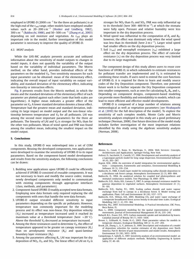
Fig. 8. Mean and standard deviation of elem

reached (when LAI is around 6), and a further increase of LAI causeda decrease of Vd. Contrary to this result, the LAI in this study didn’tcause a decrease in Vd. To isolate the effect of LAI on the modeloutput, a local sensitivity analysis was performed. In this technique,UFORE-Dwas run 100 times with only LAI varied within its possiblerange and other parameters fixed at their averages. Fig. 4(a) shows

entary effects of each parameter on Vd.

S. Hirabayashi et al. / Environmental Modelling & Software 26 (2011) 804e816 813

the result for NO2, O3, and SO2 in which Vd increases as LAIincreases. This difference was caused due to different calculationsof rs in this study and Mészáros et al.’s (2009). Mészáros et al.(2009) treated the entire canopy as one “big-leaf” and gs for theentire canopy was represented as a function of average sunlit/shaded LAI and PAR throughout the canopy.

gs ¼ LAIsunrsðPARsunÞ þ

LAIshadersðPARshadeÞ

(16)

As noted in Mészáros et al. (2009), insufficient parameterization ofPAR in their study caused a rapid decrease in both PARsun andPARshade as LAI increased. For both sunlit and shaded leaves, rs wasdetermined based solely on PAR and constant values. Therefore,a decrease in PAR directly affected an increase in rs. In Eq. (16), themagnitude of LAI increase may have been greater than that of rsincrease up to LAI’s threshold value of 6, and as a result gs and Vd

increased. When the LAI passed its threshold, however, themagnitude of rs increase may have become greater than that of LAIincrease, and thus gs and Vd became smaller.

Herewe divided the canopy into sublayers and gs for the canopywas estimated based on values for each layer. Fig. 5(a)e(f) presentsvertical profiles of PAR, LAI, and gs for sunlit and shaded leavescommonly calculated for NO2, O3, and SO2 by our model whenLAI¼ 2.5, 5, 7.5, and 10. The vertical axis, LAIj/LAI, representsvertical layers of the canopy with 1.0 and near 0.0 representing thebottom and the top of the canopy, respectively. As shown in Fig. 5(a)and (b), both PARsun and PARshade in each layer decreased as LAIincreased, but in much smaller magnitude than Mészáros et al.’s(2009). LAIsun was larger near the top of the canopy for larger LAI,though near the canopy bottom LAIsun became smaller (Fig. 5(c))since fewer leaves receive direct sunlight due to denser upperleaves; LAIshade increased as LAI increased, especially at the bottomof the layer (Fig. 5(d)). gs,sun was estimated as constant for sunlitleaves (Fig. 5(e)) regardless of LAI and canopy layers, whereasgs,shade decreased for larger LAI (Fig. 5(f)). With Eq. (9), gs wasweighted with LAI for sunlit/shaded leaves in each layer andsummed up throughout the layers to estimate gs for the entirecanopy. As a result, rs for the entire canopy was estimated as shownin Fig. 4(b). Although the magnitude of rs decrease got smaller withlarger LAI, rs never increased. Similarly, the magnitude of Vdincrease became smaller as LAI increased, though a decrease in Vddid not occur (Fig. 4(a)).

PAR has an important role in determining Vd by influencing theopening and closing of leaf stomata (Brook et al., 1999). PAR on thetop of the canopy is divided into PARsun and PARshade in each layer toestimate rs. The scatterplot (Fig. 3(b)) indicates a non-linear effect ofthe PAR on Vd for NO2. O3 and SO2 exhibited similar results (notshown here). The local sensitivity analysis of PAR for NO2 showedthat Vd increased as PAR increased until around 300e400Wm�2

(Fig. 6 (a)). This result agrees with the study by Brook et al. (1999),which reported that once the stomata were open the magnitude ofPAR became less important for Vd (i.e. stomatal opening peakedwithrelatively low levels of PAR). Wu et al. (2003) estimated that plantsreach their light saturation point at about 800Wm�2 of global solarradiation. As PAR is calculated as 46 percent of the global solarradiation (Norman, 1982; Monteith and Unsworth, 1990), thisthreshold is equivalent to a PAR of 368Wm�2, and is in goodagreement with the result presented here.

As can be seen in Fig. 3(c), (d), and Table 3, pressure, whichaffects rs through the computation of solar radiation components,PARdir and PARdiff appeared to have no relationship with Vd. Rela-tive humidity, which influences rs through the derivation of gs, hada near linear effect on Vd. Wu et al. (2003) analyzed the effects ofrelative humidity ranging from 0 to 100% on the flux of O3 and SO2.

The flux increased non-linearly with larger relative humidity untilit reached a maximum at a relative humidity of 100%. As shown inFig. 6(b), a similar behavior as reported by Wu et al. (2003) wasobserved in our local sensitivity analysis.

Temperature appeared to have a non-linear effect on Vd basedon the scatterplot in Fig. 3(e). Temperature is used to calculate allthree resistances in Eq. (2). To examine the effect of temperature oneach resistance, resistances calculated in the LHS-MC analysis wereplotted in Fig. 6(d) and (e). Ra and Rb appeared to vary independentof temperature, and the magnitude of variability was smaller thanthat of Rc. Rc had larger variability, and seemed to decrease astemperature rose up to around 20 (�C) and increased afterwards.Fig. 6(c) shows the change in Vd against the change in temperatureobtained by the local sensitivity analysis. Vd increased as temper-ature increased until about 20 �C, and further increases intemperature caused decreases in Vd. This result indicates that themaximum Vd occurs at an optimal temperature where the stomatalconductance is not limited (Wu et al., 2003; Mészáros et al., 2009).

Fig. 3(f) suggested that the relationship between Vd and windspeed was not linear. In this figure, the distribution can be dividedinto plots for the minimum to 2 m s�1 of wind speed, whereVd rapidly increased, and plots for wind speed larger than 2 m s�1,where Vd gradually increased. Wind speed primarily affects Ra andRb; the increase in turbulence that accompanies increasing windspeeds resulted in decreased Ra, whereas the increase in frictionvelocity due to the increase in wind speed resulted in decreased Rb.Fig. 6(f) presents scatterplots between wind speed and Ra, Rb, andRc. When the wind speed was less than 2 m s�1, large Ra and Rbwere dominant in determining the small Vd values shown in Fig. 3(f), and these resistances rapidly decreased as wind speedincreased. Rc didn’t appear to be affected by wind.

In several models, rm, rt, and rsoil are parameterized witha constant value. The range of rm for the three air pollutants istypically from 0 to 100 sm�1 (Hosker and Lindberg, 1982;Baldocchi, 1988; Wesely, 1989; Zhang et al., 2002). rt is typicallyset to much larger values, and ranges from 20,000 to 40,000 sm�1

for NO2 (Wesely, 1989; Mészáros et al., 2009), from 2000 to10,000 sm�1 for O3 (Wesely, 1989; Zhang et al., 2003), and from2000 to 8000 sm�1 for SO2 (Baldocchi, 1988; Wesely, 1989; Zhanget al., 2003). Typical rsoil for the three air pollutants is from 20 to2000 sm�1 (Hosker and Lindberg, 1982; Baldocchi, 1988; Meyersand Baldocchi, 1993; Zhang et al., 2003). UFORE-D also employedconstant values for rm, rt, and rsoil. To explore the effects of theseresistances on Vd, local sensitivity analyses were performed, inwhich only one resistance value varied across its possible range, theother resistances remained at their constant value, and otherparameters fixed at their average values presented in Table 1. rm, rt,and rsoil determine Rc (Eq. (5)), which in turn determines Vd (Eq.(2)). Fig. 7 presents the results for NO2, O3, and SO2. In general, theconstant values set to each resistance had a large effect on deter-mining the typical value of Vd. For example in Fig. 7(a), rm for NO2,O3, and SO2 was set to 100 sm�1,10 sm�1, and 0 sm�1, respectively.Corresponding Vd is 0.48 cm s�1, 0.75 cm s�1, and 0.72 cm s�1,respectively, which are close to the hourly average Vd at noon forthe leaf-on season (Fig. 2). Choosing different values for the resis-tances will impact Vd; however, each resistance has a varied impact.Within the possible range of rm, decrease in Vd for NO2, O3, and SO2was relatively large (39%, 37%, and 34%, respectively). Contrarily,changes in rt caused very small changes in Vd because its value ismuch larger than rm, and thus, the effect of rt on the model outputwas minimal. Over the possible range of rsoil, Vd decreased rapidlyas rsoil increased up to about 1000 sm�1, then after this valuedecreases in Vd became much smaller. Overall, the decrease in Vdfor NO2, O3, and SO2 (69%, 55%, and 55%, respectively) was largestamong the three resistances. While the constant values for rsoil

S. Hirabayashi et al. / Environmental Modelling & Software 26 (2011) 804e816814

employed in UFORE-D (2000 sm�1 for the three air pollutants) is atthe high end of the rsoil range, other models have employed smallervalues such as 20e200 sm�1 (Hosker and Lindberg, 1982),300 sm�1 (Baldocchi, 1988), and 50e500 sm�1 (Zhang et al., 2003)depending on soil moisture and vegetation. As rsoil plays animportant role in the model, further investigation of this modelparameter is necessary to improve the quality of UFORE-D.

4.3. MOAT analysis

While the LHS-MC analysis presents accurate and unbiasedinformation about the sensitivity of model outputs to changes inmodel inputs, it does not quantify the variability of the outputbased on the variability of individual parameters. The Morrismethod, on the other hand, provides individual effects of theparameters on the modeled Vd. Two sensitivity measures for eachinput parameter can be obtained: mean of the elementary effect,indicating the overall impact of input variability on output vari-ability, and standard deviation of the elementary effect, indicatingnon-linearity or interaction effects.

Fig. 8 presents results from the Morris method, in which themeans and the standard deviations of the elementary effect of eachparameter are plotted against each other (note that both scales arelogarithmic). A higher mean indicates a greater effect of theparameter on Vd. A lower standard deviation denotes a linear effect.Temperature had the greatest mean and standard deviation, indi-cating its large impact on model output and the non-linear rela-tionship between temperature and Vd for all pollutants. LAI wasamong the second most important parameters for the three airpollutants. The linearity of LAI and Vd is stronger for NO2 than forthe other two pollutants. Mean of wind speed and PAR was foundamong the smallest mean, indicating the smallest impact on themodel output.

5. Conclusions

In this study, UFORE-D was redeveloped into a set of COMcomponents. Reusing the developed components, two applicationswere developed to examine the sensitivity of UFORE-D to its inputparameters. Based on the component-based model developmentand results from the sensitivity analyses, the following conclusionscan be drawn:

1. Building new applications upon UFORE-D could be efficientlyachieved if UFORE-D consisted of reusable components. It wasnot necessary to learn and modify the source codes; instead,newly developed components only needed to communicatewith existing components through appropriate interfaces(class, methods, and parameters).

2. Component-basedUFORE-D readily accepted newdata formats.Employing new data formats only required replacing the oldcomponents with ones that handle the new data formats.

3. UFORE-D output revealed different sensitivity to inputparameters depending on the specific air pollutants. However,temperature was commonly important for the modelingprocess and its effect was non-linear. Dry deposition velocity(Vd) increased as temperature increased until it reached itsmaximum value at a threshold temperature (here w20 �C).Above the threshold Vd decreased as temperature increased.

4. Among the three resistances used to determine Vd, the effect oftemperature appeared to be greater on canopy resistance (Rc)than on aerodynamic resistance (Ra) and quasi-laminarboundary layer resistance (Rb).

5. Among the parameters affecting Rc, LAI was important for drydeposition of NO2, O3, and SO2. The linear effect of LAI on Vd is

stronger for NO2 than O3 and SO2. PAR was only influential upto its threshold (here 300e400 Wm�2) at which the stomatawere fully open. Pressure and relative humidity were lessimportant in the dry deposition process.

6. Wind speed was influential to the computation of Ra and Rb;however, the effect was dominant only when the wind speedwas less than its threshold (here 2 m s�1). Larger wind speedhad smaller effects on the dry deposition process.

7. Soil (rsoil) and mesophyll resistances (rm) exhibited a largeeffect on the dry deposition process. The effect of cuticularresistance (rt) on the dry deposition process was very limiteddue to its large magnitude.

The component design of this study allows users to reuse corefunctions of UFORE-D, in which submodels to estimate resistancesfor pollutant transfer are implemented and Vd is estimated bycombining these results. If users need to extend the core functionsof UFORE-D, it is required for them to learn and modify sourcecodes of the Dry Deposition component. Therefore, one potentialfuture work is to further separate the Dry Deposition componentinto smaller components, such as ones for calculating Ra, Rb, and rs.Depending on component designs, component-based modelingcan provide more flexibility and extendability to models, which canlead to more efficient and effective model developments.

UFORE-D is composed of a large number of relations amongmeteorological as well as vegetation parameters (see Hirabayashiet al. (2010) for the full description of the model). To explore thesensitivity of such complex models, Monte Carlo and Morrissensitivity analyses employed in this study are a good preliminarytechnique (Norman, 2008). One future direction of the model studyincludes further investigation of the most important relationsidentified by this study using the algebraic sensitivity analysis(Norman, 2008).

References

Alonso, G., Casati, F., Kuno, H., Machiraju, V., 2004. Web Services: Concepts,Architectures and Applications. Springer-Verlag, New York.

Anfossi, D., Sacchettit, D., Castelli, S.T., 1996. Development and sensitivity analysis ofa Lagrangian particle model for long range dispersion. Environmental Software10 (4), 263e287.

Argent, R.M., 2004. An overview of model integration for environmental applica-tions e components, frameworks and semantics. Environmental Modelling &Software 19 (3), 219e234.

Baldocchi, D., 1988. A multi-layer model for estimating sulfur dioxide deposition toa deciduous oak forest canopy. Atmospheric Environment 22 (5), 869e884.

Baldocchi, D., 1994. An analytical solution for coupled leaf photosynthesis andstomatal conductance models. Tree Physiology 14, 1069e1079.

Baldocchi, D.D., Hicks, B.B., Camara, P., 1987. A canopy stomatal resistance model forgaseous deposition to vegetated surfaces. Atmospheric Environment 21 (1),91e101.

Baldocchi, D.D., Harley, P.C., 1995. Scaling carbon dioxide and water vapourexchange from leaf to canopy in a deciduous forest. II. Model testing andapplication. Plant, Cell and Environment 18 (10), 1157e1173.

Baldocchi, D.D., Wilson, K.B., 2001. Modeling CO2 and water vapor exchange ofa temperate broadleaved forest across hourly to decadal time scales. EcologicalModelling 142 (1e2), 155e184.

Barnsley, M.J., 2007. Environmental Modeling: A Practical Introduction. CRC Press,Boca Raton, FL.

Bian, L., 2000. Component modeling for the spatial representation of wildlifemovements. Journal of Environmental Management 59 (4), 235e245.

Bidwell, R.G., Fraser, D.E., 1972. Carbon monoxide uptake and metabolism by leaves.Canadian Journal of Botany 50 (7), 1435e1439.

Breuer, L., Eckhardt, K., Frede, H.-G., 2003. Plant parameter values for models intemperate climates. Ecological Modelling 169 (2e3), 237e293.

Brook, J.R., Zhang, L., Li, Y., Johnson, D., 1999. Description and evaluation of a modelof deposition velocities for routine estimates of dry deposition over NorthAmerica. Part II: Review of past measurements and model results. AtmosphericEnvironment 33 (30), 5053e5070.

Campolongo, F., Saltelli, A., 1997. Sensitivity analysis of an environmental model: anapplication of different analysis methods. Reliability Engineering & SystemSafety 57, 49e69.

S. Hirabayashi et al. / Environmental Modelling & Software 26 (2011) 804e816 815

Campolongo, F., Cariboni, J., Saltelli, A., 2007. An effective screening design forsensitivity analysis of large models. Environmental Modelling & Software22 (10), 1509e1518.

Caton, B.P., Foin, T.C., Hill, J.E., 1999. A plant growth model for integrated weedmanagement in direct-seeded rice I. Development and sensitivity analyses ofmonoculture growth. Field Crops Research 62 (2e3), 129e143.

Chappell, D., 1996. Understanding ActiveX and OLE: A Guide for Developers &Managers. Microsoft Press, Redmond, WA.

Colbeck, I., Harrison, R.M., 1985. Dry deposition of ozone: some measurements ofdeposition velocity and of vertical profiles to 100 meters. Atmospheric Envi-ronment 19 (11), 1807e1818.

Collatz, G.J., Ball, J.T., Grivet, C., Berry, J.A., 1991. Physiological and environmentalregulation of stomatal conductance, photosynthesis and transpiration: a modelthat includes a laminar boundary layer. Agricultural and Forest Meteorology54 (2e4), 107e136.

Currie, B.A., Bass, B., 2008. Estimates of air pollution mitigation with green plantsand green roofs using the UFORE model. Urban Ecosystems 11 (4), 409e422.

Davidson, C.I., Wu, Y.L., 1990. Dry deposition of particles and vapors. In:Lindberg, S.E., Page, A.L., Norton, S.A. (Eds.), Acidic Precipitation. Sources,Deposition, and Canopy Interactions, vol. 3. Springer-Verlag, New York,pp. 103e216.

Deutsch, B., Whitlow, H., Sullivan, M., Savineau, A., 2005. Re-greening Washington,DC: A Green Roof Vision Based on Quantifying Storm Water and Air QualityBenefits. http://www.greenroofs.org/resources/greenroofvisionfordc.pdf(accessed February 2009).

Dyer, A.J., Bradley, C.F., 1982. An alternative analysis of flux gradient relationships.Boundary-Layer Meteorology 22 (1), 3e19.

Farquhar, G.D., von Caemmerer, S., Berry, J.A., 1980. A biochemical model ofphotosynthetic CO2 assimilation in leaves of C3 species. Planta 149 (1), 78e90.

Fowler, D., 1985. Deposition of SO2 onto plant canopies. In: Winner, W.E.,Mooney, H.A., Goldstein, R.A. (Eds.), Sulfur Dioxide and Vegetation. StanfordUniversity Press, Stanford, CA, pp. 389e402.

Fowler, D., Cape, J.N., 1983. Dry deposition of SO2 onto a Scots pine forest. In:Pruppacher, H.R., Semonin, R.G., Slinn, W.G.N. (Eds.), Precipitation Scavenging,Dry Deposition and Resuspension. Elsevier, New York, pp. 763e773.

Garland, J.A., Branson, J.R., 1977. The deposition of sulfur dioxide to pine forestassessed by a radioactive tracer method. Tellus 29, 445e454.

Greenhut, G.K., 1983. Resistance of a pine forest to ozone uptake. Boundary-LayerMeteorology 27 (4), 387e391.

Hamby, D.M., 1994. A review of techniques for parameter sensitivity analysis ofenvironmental models. Environmental Monitoring and Assessment 32,135e154.

Harley, P.C., Thomas, R.B., Reynolds, J.F., Strain, B.R., 1992. Modelling photosynthesisof cotton grown in elevated CO2. Plant, Cell and Environment 15 (3), 271e282.

Harley, P.C., Baldocchi, D.D., 1995. Scaling carbon dioxide and water vapourexchange from leaf to canopy in a deciduous forest. I. Leaf model parameteri-zation. Plant, Cell and Environment 18 (10), 1146e1156.

He, C., Larsen, D.R., Mladenoff, D.J., 2002. Exploring component-based approachesin forest landscape modeling. Environmental Modelling & Software 17 (6),519e529.

Helton, J.C., 1993. Uncertainty and sensitivity analysis techniques for use inperformance assessment for radioactive waste disposal. Reliability Engineering& Systems Safety 42 (2e3), 327e367.

Hermann, A.J., Stabeno, P.J., Haidvogel, D.B., Musgrave, D.L., 2002. A regional tidal/subtidal circulation model of the southeastern Bering Sea: development,sensitivity analyses and hindcasting. Deep-Sea Research II 49 (26), 5945e5967.

Hosker Jr., R.P., Lindberg, S.E., 1982. Review: atmospheric deposition and plantassimilation of gases and particles. Atmospheric Environment 16 (5), 889e910.

Hirabayashi, S., Kroll, C.N., Nowak, D.J., 2010. UFORE-D Model Descriptions. http://www.itreetools.org/resources/archives.php (accessed August 2010).

Killus, J.P., Meyer, J.P., Durran, D.R., Anderson, G.E., Jerskey, T.N., Reynolds, S.D.,Ames, J., 1984. Continued research in mesoscale air pollution simulationmodeling. In: Refinements in Numerical Analysis, Transport, Chemistry, andPollutant Removal, vol. V. United States Environmental Protection Agency,Research Triangle Park, NC. Publ. EPA/600/3.84/095a.

Leuning, R., 1990. Modelling stomatal behavior and photosynthesis of eucalyptusgrandis. Australian Journal of Plant Physiology 17 (2), 159e175.

Liepmann, D., Stephanopoulos, G., 1985. Development and global sensitivity anal-ysis of a closed ecosystem model. Ecological Modelling 30 (1e2), 13e47.

Lorenz, R., Murphy, C.E., 1985. The dry deposition of sulfur dioxide on a loblolly pineplantation. Atmospheric Environment 19 (5), 797e802.

Lovett, G.M., 1994. Atmospheric deposition of nutrients and pollutants in NorthAmerica: an ecological perspective. Ecological Applications 4 (4), 629e650.

Lovett, G.M., Lindberg, S.E., 1984. Dry deposition and canopy exchange in a mixedoak forest as determined by analysis of throughfall. Journal of Applied Ecology21 (3), 1013e1027.

MacDougall, M., Smith, R.I., Scott, E.M., 2005. Comprehensive sensitivity analysis ofan SO2 deposition model for three measurement sites: consequences for SO2deposition fluxes. Atmospheric Environment 39, 5025e5039.

MacKerron, D.K.L., Waister, P.D., 1985. A simple model of potato growth and yield.Part l. Model development and sensitivity analysis. Agricultural and ForestMeteorology 34 (2e3), 241e252.

Maxwell, E.L., 1998. METSTAT e the solar radiation model used in the production ofthe national solar radiation database (NSRDB). Solar Energy 62 (4), 263e279.

McMahon, T.A., Denison, P.J., 1979. Empirical atmospheric deposition parameters ea survey. Atmospheric Environment 13, 571e585.

Mészáros, R., Zsély, I.Gy., Szinyei, D., Vincze, Cs, Lagzi, I., 2009. Sensitivity analysis ofan ozone deposition model. Atmospheric Environment 43 (3), 663e672.

Meyers, T.P., Baldocchi, D.D., 1993. Trace gas exchange above the floor of a decid-uous forest 2. SO2 and O3 deposition. Journal of Geophysical Research 98 (D7),12631e12638.

Microsoft Developer Network (MSDN), 2009. COM Clients and Servers. http://msdn.microsoft.com/en-us/library/ms683835(VS.85).aspx (accessed March 2009).

Monteith, J.L., Unsworth, M.H., 1990. Principles of Environmental Physics. EdwardArnold, New York.

Morris, M.D., 1991. Factorial sampling plans for preliminary computational exper-iments. Technometrics 33 (2), 161e174.

Murphy, C.E., Sigmon, J.T., 1990. Dry deposition of sulfur and nitrogen oxide gases toforest vegetation. In: Lindberg, S.E., Page, A.L., Norton, S.A. (Eds.), AcidicPrecipitation. Sources, Deposition, and Canopy Interactions, vol. 3. Springer-Verlag, New York, pp. 217e240.

National Aeronautics and Space Administration (NASA), 2009. Remote SensingTutorial, Section 3 Vegetation Applications e Agriculture, Forestry, and Ecology.http://rst.gsfc.nasa.gov/Sect3/Sect3_1.html (accessed January 2009).

National Climate Data Center (NCDC), 2008. World’s Largest Archive of ClimateData: National Climate Data Center. http://www.ncdc.noaa.gov/oa/ncdc.html(accessed September 2008).

National Oceanic & Atmospheric Administration (NOAA), 2010. Trends inAtmospheric Carbon Dioxide e Globally Averaged Marine Surface AnnualMean Data. ftp://ftp.cmdl.noaa.gov/ccg/co2/trends/co2_annmean_gl.txt(accessed November 2010).

Norman, J.M., 1980. Interfacing leaf and canopy light interception models. In:Hesketh, J.D., Jones, J.W. (Eds.), Predicting Photosynthesis for EcosystemModels, vol. II. CRC Press, Boca Raton, FL, pp. 49e67.

Norman, J.M., 1982. Simulation of microclimates. In: Biometeorology in IntegratedPest Management, 65e99. Proceedings of a Conference on Biometeorology andIntegrated Pest Management, Davis, CA.

Norton, J.P., 2008. Algebraic sensitivity analysis of environmental models. Envi-ronmental Modelling & Software 23, 963e972.

Nowak, D.J., McHale, P.J., Ibarra, M., Crane, D., Stevens, J., Luley, C., 1998. Modelingthe effects of urban vegetation on air pollution. In: Gryning, S.E.,Chaumerliac, N. (Eds.), Air Pollution Modeling and its Application XII. PlenumPress, New York, pp. 399e407.

Nowak, D.J., Crane, D.E., 2000. The urban forest effects (UFORE) model: quantifyingurban forest structure and functions. In: Hansen, M., Burk, T. (Eds.), IntegratedTools for Natural Resources Inventories in the 21st Century: Proceedings of theIUFRO Conference. United States Department of Agriculture, Forest Service,North Central Research Station, St. Paul, MN, pp. 714e720. Gen. Tech. Rep. NC-212.

Nowak, D.J., Civerolo, K.L., Rao, S.T., Sistla, G., Juley, C.J., Crane, D.E., 2000.A modeling study of the impact of urban trees on ozone. Atmospheric Envi-ronment 34 (10), 1601e1613.

Nowak, D.J., Crane, D.E., Stevens, J.C., 2006. Air pollution removal by urban treesand shrubs in the United States. Urban Forestry & Urban Greening 4 (3e4),115e123.

Pataki, D.E., Bowling, D.R., Ehleringer, J.R., 2003. Seasonal cycle of carbon dioxideand its isotopic composition in an urban atmosphere: anthropogenic andbiogenic effects. Journal of Geophysical Research 108 (D23) ACH 8e1eACH8e8.

Pederson, J.R., Massman, W.J., Mahrt, L., Delany, A., Oncley, S., Hartog, G.den,Neumann, H.H., Mickle, R.E., Shaw, R.H., Paw, U.K.T., Grantz, D.A.,MacPherson, J.I., Desjardins, R., Schuepp, P.H., Pearson Jr., R., Arcado, T.E., 1995.California ozone deposition experiment: methods, results, and opportunities.Atmospheric Environment 29 (21), 3115e3132.

Pohlert, T., Huisman, J.A., Breuer, L., Frede, H.-G., 2007. Integration of a detailedbiogeochemical model into SWAT for improved nitrogen predictionsdmodeldevelopment, sensitivity, and GLUE analysis. Ecological Modelling 203 (3e4),215e228.

Ravalico, J.K., Maier, H.R., Dandy, G.C., Norton, J.P., Croke, B.F.W., 2005. A comparisonof sensitivity analysis techniques for complex models for environmentmanagement. In: Zerger, A., Argent, R.M. (Eds.), International Congress onModelling and Simulation: Advances and Applications for Management andDecision Making, Melbourne, 12e15 December, pp. 2533e2539.

Saltelli, A., Chan, K., Scot, E.M., 2000. Sensitivity Analysis. John Wiley & Sons, WestSussex, UK.

Simpson, D., Touvinen, J.P., Emberson, L., Ashmore, M.R., 2003. Characteristics of anozone deposition module II: sensitivity analysis. Water, Air, and Soil Pollution143, 123e137.

Smith, R.I., Fowler, D., Sutton, M.A., Flechard, C., Coyle, M., 2000. Regional estima-tion of pollutant gas dry deposition in the UK: model description, sensitivityanalyses and outputs. Atmospheric Environment 34, 2757e3777.

Taylor Jr., G.E., Hanson, P.J., Baldocchi, D.D., 1988. Pollutant deposition to individualleaves and plant canopies: sites of regulation and relationship to injury. In:Heck, W.W., Taylor, O.C., Tingey, D.T. (Eds.), Assessment of Crop Loss From AirPollutants. Elsevier Applied Science, London, England, pp. 227e258.

United States Environmental Protection Agency (US EPA), 1995. PCRAMMET User’sGuide. United States Environmental Protection Agency, Research TrianglePark, NC.

S. Hirabayashi et al. / Environmental Modelling & Software 26 (2011) 804e816816

United States Environmental Protection Agency (US EPA), 2009. TechnologyTransfer Network (TTN): Air Quality System (AQS). http://www.epa.gov/ttn/airs/airsaqs/ (accessed February 2009).

van Griensven, A., Meixner, T., Grunwald, S., Bishop, T., Diluzio, M., Srinivasan, R.,2006. A global sensitivity analysis tool for the parameters of multi-variablecatchment models. Journal of Hydrology 324 (1e4), 10e23.

van Ulden, A.P., Holtslag, A.A.M., 1985. Estimation of atmospheric boundary layerparameters for diffusion application. Journal of Climatology and AppliedMeteorology 24 (11), 1196e1207.

Venkatram, A., 1980. Estimating the Monin-Obukhov length in the stable boundarylayer for dispersion calculations. Boundary-Layer Meteorology 19 (4), 481e485.

Vitousek, P.M., Mooney, H.A., Lubchenco, J., Melillo, J.M., 1997. Human dominationof earth’s ecosystems. Science 277, 494e499.

Weiler, M., 2005. An infiltration model based on flow variability in macropores:development, sensitivity analysis and applications. Journal of Hydrology 310(1e4), 294e315.

Weiss, A., Norman, J.M., 1985. Partitioning solar radiation into direct and diffuse,visible and near-infrared components. Agricultural and Forest Meteorology34 (2e3), 205e213.

Wesely, M.L., 1989. Parameterization of surface resistances to gaseous dry deposi-tion in regional-scale numerical models. Atmospheric Environment 23 (6),1293e1304.

Whittaker, R.H., Woodwell, G.M., 1967. Surface area relations of woody plants andforest communities. American Journal of Botany 54 (8), 931e939.

Wilson, K.B., Baldocchi, D.D., Hanson, P.J., 2001. Leaf age affects the seasonal patternof photosynthetic capacity and net ecosystem exchange of carbon in a decid-uous forest. Plant, Cell and Environment 24 (6), 571e583.

Wu, Y., Brashers, B., Finkelstein, P.L., Pleim, J.E., 2003. A multilayer biochemical drydeposition model 2. Model evaluation. Journal of Geophysical Research 108 (1)ACH2e1 e ACH2e16.

Zádor, J., Zsély, I.Gy., Turányi, T., Ratto, M., Tarantola, S., Saltelli, A., 2005. Local andglobal uncertainty analyses of a methane flame model. Journal of PhysicalChemistry 109 (43), 9795e9807.

Zhang, L., Moran, M.D., Makar, P.A., Brook, J.R., Gong, S., 2002. Modelling gaseousdry deposition in AURAMS: a unified regional air-quality modelling system.Atmospheric Environment 36 (3), 537e560.

Zhang, L., Brook, J.R., Vet, R., 2003. A revised parameterization for gaseous drydeposition in air-quality models. Atmospheric Chemistry and Physics 3 (6),2067e2082.

Ziehn, T., Tomlin, A.S., 2008. Global sensitivity analysis of a 3D street canyonmodeldPart I: The development of high dimensional model representations.Atmospheric Environment 42 (8), 1857e1873.

Zinke, P.J., 1967. Forest interception studies in the United States. In: Sopper, W.E.,Lull, H.W. (Eds.), Forest Hydrology. Pergamon Press, Oxford, UK, pp. 137e161.