Complexity as a Barrier to Annuitization: Do Consumers...
50
1 Complexity as a Barrier to Annuitization: Do Consumers Know How to Value Annuities? March 12, 2013 Jeffrey R. Brown Arie Kapteyn Department of Finance Center for Economic and Social Research University of Illinois University of Southern California 515 E. Gregory Drive 12015 Waterfront Drive Champaign, IL 61820 Playa Vista, CA 90094-2536 and NBER [email protected] [email protected] Erzo F. P. Luttmer Olivia S. Mitchell Department of Economics The Wharton School 6106 Rockefeller Center University of Pennsylvania Dartmouth College 3620 Locust Walk, 3000 SH-DH Hanover, NH 03755 Philadelphia, PA 19104 and NBER and NBER [email protected] [email protected] The research reported herein was performed pursuant to a grant from the U.S. Social Security Administration (SSA) funded as part of the Financial Literacy Consortium. The authors also acknowledge support provided by the Pension Research Council and Boettner Center at the Wharton School of the University of Pennsylvania, and the RAND Corporation. The authors thank Caroline Tassot and Yong Yu for superb research assistance, and Tim Colvin, Tania Gutsche, and Bas Weerman for their invaluable comments and assistance on the project. Brown is a Trustee of TIAA and has served as a speaker, author or consultant for a number of financial services organizations, some of which sell annuities and other retirement income products. Mitchell is a Trustee of the Wells Fargo Advantage Funds and has received research support from TIAA-CREF. The opinions and conclusions expressed herein are solely those of the authors and do not represent the opinions or policy of SSA, any agency of the Federal Government, or any other institution with which the authors are affiliated. ©2013 Brown, Kapteyn, Luttmer and Mitchell. All rights reserved.
Transcript of Complexity as a Barrier to Annuitization: Do Consumers...

1
Complexity as a Barrier to Annuitization:
Do Consumers Know How to Value Annuities?
March 12, 2013 Jeffrey R. Brown Arie Kapteyn Department of Finance Center for Economic and Social Research University of Illinois University of Southern California 515 E. Gregory Drive 12015 Waterfront Drive Champaign, IL 61820 Playa Vista, CA 90094-2536 and NBER [email protected] [email protected] Erzo F. P. Luttmer Olivia S. Mitchell Department of Economics The Wharton School 6106 Rockefeller Center University of Pennsylvania Dartmouth College 3620 Locust Walk, 3000 SH-DH Hanover, NH 03755 Philadelphia, PA 19104 and NBER and NBER [email protected] [email protected] The research reported herein was performed pursuant to a grant from the U.S. Social Security Administration (SSA) funded as part of the Financial Literacy Consortium. The authors also acknowledge support provided by the Pension Research Council and Boettner Center at the Wharton School of the University of Pennsylvania, and the RAND Corporation. The authors thank Caroline Tassot and Yong Yu for superb research assistance, and Tim Colvin, Tania Gutsche, and Bas Weerman for their invaluable comments and assistance on the project. Brown is a Trustee of TIAA and has served as a speaker, author or consultant for a number of financial services organizations, some of which sell annuities and other retirement income products. Mitchell is a Trustee of the Wells Fargo Advantage Funds and has received research support from TIAA-CREF. The opinions and conclusions expressed herein are solely those of the authors and do not represent the opinions or policy of SSA, any agency of the Federal Government, or any other institution with which the authors are affiliated. ©2013 Brown, Kapteyn, Luttmer and Mitchell. All rights reserved.

2
Complexity as a Barrier to Annuitization: Do Consumers Know How to Value Annuities?
Jeffrey R. Brown, Arie Kapteyn, Erzo F.P. Luttmer, and Olivia S. Mitchell
Abstract This paper provides experimental evidence that individuals have difficulty valuing annuities, and this difficulty – rather than a preference for lump sums – can help explain observed low levels of annuity purchases. Although the median price at which people are willing to sell an annuity is close to median actuarial values, this masks notable heterogeneity in responses including substantial numbers of respondents whose responses are difficult to reconcile with optimizing behavior under any reasonable parameter assumptions. We also discover that people are willing to pay substantially less to buy a larger annuity, a result not due to liquidity constraints or endowment effects. Strikingly, we also learn that individual responses to the buy versus sell decisions are negatively correlated, an effect that is stronger for the less financially sophisticated. Our findings are consistent with boundedly rational consumers who adopt a “buy low, sell high” heuristic when faced with a complex trade-off. Moreover, at the margin, subjective valuations vary nearly one-for-one with actuarial values but are uncorrelated with utility-based measures designed to measure the insurance value of annuities. This supports the hypothesis that people use simplifying heuristics to think about annuities, rather than engaging in optimizing behavior. Results also underscore the difficulty of explaining the cross-sectional variation in annuity valuations using standard empirical models. Our findings raise doubt about whether most consumers can make optimal decisions about annuitization.

3
Complexity as a Barrier to Annuitization: Do Consumers Know How to Value Annuities?
1. Introduction
An enduring empirical puzzle in the economics literature is why individuals so rarely
purchase annuities to insure against length-of-life uncertainty, despite the substantial value that
annuities have been shown to provide in standard life cycle models. Following Yaari’s (1965)
early paper establishing conditions under which full annuitization proves optimal, many
subsequent researchers have sought to solve what has been dubbed the “annuity puzzle,” a term
that refers to the question of why few ‘real world’ consumers annuitize their retirement wealth.
That research, discussed in more detail below, explores several plausible explanations ranging
from supply-side market imperfections (e.g., adverse selection, aggregate risk, or incomplete
annuity markets) to rational demand-side limitations (e.g., bequest motives, the availability of
formal and informal substitutes, or the presence of insured expenditure shocks). In general,
however, it appears that no single factor can explain the limited demand for payout annuities;
moreover, while combining many factors into one model can generate limited annuity demand,
such an approach typically comes at the cost of creating new puzzles.
Of late, researchers have begun to explore psychological barriers to annuitization in both
theoretical and experimental studies.1 The present paper contributes to this nascent literature by
providing evidence consistent with the hypothesis that many people find it difficult to value
annuities, and that this difficulty – rather than a well-defined preference for lump sums – may
explain the observed reluctance of individuals to annuitize.
There are at least two complementary reasons that individuals may deviate from
optimizing behavior in the annuitization context. First, individuals may exhibit bounded 1 For a recent survey, see Benartzi et al. (2011).

4
rationality (Simon 1947) and thus make mistakes in the optimization process. The annuitization
decision is a complex one because it combines decision-making under uncertainty and the
making of choices that have distant consequences, each of which is known to be difficult
(Beshears et al. 2008). Determining the optimal mix of annuitized and non-annuitized resources
requires that one forecast mortality, capital market returns, inflation, future expenditures, income
uncertainty, and other factors, and appropriately weigh these relative to one’s current assessment
of future preferences. The typical individual who is unable to solve a complex dynamic
programming problem may therefore find it difficult to evaluate the expected lifetime utility
consequences of annuitization. If so, then as Benartzi and Thaler (2002, p. 1607) noted in their
study of how portfolio choices are affected by the availability of irrelevant options, people may
“not really have well-formed preferences, but rather construct preferences when choices are
elicited. Since the form of the elicitation can affect the choices people make, there is not a single
preference ordering that can be clearly identified.” The recent evidence on how framing affects
the perceived desirability of annuities is consistent with this view.2
Second, as noted by Kling, Phaneuf, and Zhao (2012: 12) in their overview of contingent
valuation methods, “rationality may be the result of repeated participation in markets …
departures from rationality can therefore be aggravated by complex or unfamiliar decision
environments and uncertainties, which can often result in rule-of-thumb behaviors.” Beshears et
al. (2008) made a similar point, namely that limited personal experience can create a wedge
between revealed preferences (i.e., those that might be inferred from our actions) and true
underlying preferences. Bernheim (2002) also discussed how individuals who fail to save
adequately for retirement are unable to learn from experience; by the time they retire with
2 Research on framing is linked to Kahnemann and Tversky (1981); in the annuity context, see Agnew et al. (2008); Brown et al. (2008b); and Brown et al. (2013).

5
inadequate resources, they cannot return to a younger age and save more. In the present context,
most individuals have little or no experience making annuitization decisions, let alone the ability
to learn from the experience of having (or not having) an annuity later in their own lives.
Although it might be possible to learn from observing the experience of others, this does not
always happen: when Enron, WorldCom, and Global Crossing employees' 401(k) balances were
devastated due to over-investment in their employers’ stock, there was virtually no reaction by
workers at other U.S. firms to reduce their own investments in employer stock (Choi et al. 2005).
Our central hypothesis is that many people do not fully understand the lifetime utility
implications of the annuitization decision, and therefore they have difficulty forming an
appropriate assessment of the value of annuities. We provide evidence to support this hypothesis
using a randomized experiment in the American Life Panel (ALP), in which we present
individuals with hypothetical choices between a lump sum and a Social Security annuity. By
varying whether the questions elicit a compensating variation (CV) or equivalent variation (EV)
value, whether the individual is buying or selling the annuity, the size of the increments, the
order of the questions, and so on, we are able to examine the coherence and stability of the
subjective values that individuals place on the Social Security annuity. We are also able to make
use of the rich ALP database to control for potentially confounding factors such as heterogeneity
in liquidity constraints or beliefs about political risk.
We provide five pieces of evidence consistent with the hypothesis that individuals have
difficulty valuing the annuity. First, we find that even when median valuations appear
reasonable, many peoples’ implied annuity values are difficult to reconcile with optimizing
behavior under any plausible set of parameters. Second, we uncover a large divergence between
the price at which individuals are willing to buy an annuity and the price at which they are

6
willing to sell an annuity. This result is not due to liquidity constraints or endowment effects;
instead it is consistent with a simple “buy low, sell high” heuristic. Third, we show that the “buy
value” and the “sell value” are negatively correlated, particularly for the less financially
sophisticated. Fourth, we use other experimental variation to show that the implied valuations
violate the “invariance” criteria of rational decision-making, such as being sensitive to anchoring
effects. Finally, we argue that it is difficult to explain the overall cross-sectional variation in the
annuity values using theoretically attractive measures, and that that the pattern of significant
marginal valuation predictors is consistent with individuals using simple heuristics rather than
full optimization to value the trade-offs.
In addition to advancing our academic understanding of consumer behavior in this
area, our results also have considerable practical policy relevance. There is currently an active
discussion of what role payout annuities should play in defined contribution (DC) or 401(k)
pension plans, with much debate about whether and how life annuities ought to be encouraged in
such settings (Gale et al. 2008; Brown 2009); this debate in part revolves around whether
individuals are making optimal payout decisions. Moreover, many countries including the U.S.
are grappling with fiscally unsustainable pay-as-you-go public pension systems. To the extent
that households are poorly-equipped to value the annuities offered by their public pensions, this
can have implications for the political feasibility of reforms that change the benefit structure,
particularly in cases where individuals are provided a choice to accept a lump sum in lieu of
future annuity payments. The same, of course, is true with state and local public defined benefit
plans (DB) in the U.S., which also face substantial underfunding problems (Novy-Marx and
Rauh, 2011), and for which some reformers have called for a reduction in DB annuities in
exchange for lump sum contributions to defined contribution accounts (e.g., Kilgour 2006).

7
In what follows, we first summarize prior studies on the demand for annuities, including
both the neoclassical and the behavioral economics literatures. Next we describe the American
Life Panel (ALP) internet survey, a relatively representative sample of the US population, and
we outline how we elicit lump sum versus annuity preferences. Then we present the key
empirical results of the paper, followed by a number of robustness checks and further analyses
for subgroups that vary in their financial capability. We conclude with a discussion of possible
policy implications and future research questions.
2. What We Know About the Annuity Puzzle
2.1 Prior Theoretical and Simulation Research on Rational Life Annuity Demand 3
The modern economics literature on annuities has noted a set of conditions under which it
would be optimal for an individual to annuitize 100% of his wealth.4 Extensions to the theory
have demonstrated that full annuitization will be optimal under a more general set of conditions.5
More recent studies have used extended life-cycle models to measure how consumers value
payout annuities and they compute how optimal annuitization varies with other factors, including
pricing (Mitchell et al. 1999); pre-existing annuitization (Brown 2001; Dushi and Webb 2006);
risk-sharing within families (Kotlikoff and Spivak 1981; Brown and Poterba 2000); uncertain
health expenses (Turra and Mitchell 2008; Sinclair and Smetters 2004; Peijnenburg et al. 2010a, 3 Rather than providing a comprehensive review here, we instead highlight those studies most germane to the research that follows. Readers interested in the broader literature on life annuities may consult Benartzi et al. (2011); Poterba et al. (2011); Brown (2008); Horneff et al. (2007); and Mitchell et al. (1999). Note that we use the term “life annuity” because we are interested in products that guarantee income for life, as opposed to some financial products – such as “equity indexed annuities” – that are primarily used as tax-advantaged wealth accumulation devices and are rarely converted into life-contingent income. 4 The conditions included no bequest motives, time-separable utility, exponential discounting, and actuarially fair annuities (among others). 5 Davidoff et al. (2005) showed that full annuitization is optimal under complete markets with no bequest motive. Peijnenburg et al. (2010a; 2010b) found that if agents save optimally out of annuity income, full annuitization can be optimal even in the presence of liquidity needs and precautionary motives. They further find that full annuitization is suboptimal only if agents risk substantial liquidity shocks early after annuitization and do not have liquid wealth to cover these expenses. This result is robust to the presence of significant loads.

8
2010b), bequests (Brown 2001; Lockwood 2011); inflation (Brown et al. 2001, 2002); the option
value of learning about mortality (Milevsky and Young 2007); stochastic mortality processes
(Reichling and Smetters 2012; Maurer et al. 2013); and broader portfolio choice issues including
labor income and the types of assets on offer (Inkmann et al. 2011; Koijen et al. 2011; Chai et al.
2011; Horneff et al. 2009, 2010).
Our overall assessment of this neoclassical microeconomics literature is that it has not
been fully successful in resolving the annuity puzzle, even for marginal annuitization decisions
(e.g., Shepard 2011). Although some papers have been able to simulate low overall demand for
annuities (e.g., Dushi and Webb 2006; Inkmann et al. 2011; Horneff et al. 2009, 2010; Reichling
and Smetters 2012), many of the proposed annuity puzzle solutions create new puzzles. For
example, studies that rely on risk-sharing within families are unable to fully explain why the
demand for annuities does not rise after people transition from married life to widowhood.
Studies that emphasize the lack of inflation protection or actuarially unfair pricing are unable to
explain why it is so common for people to forego the opportunity to purchase higher Social
Security benefits by delaying the date of claiming (they are inflation-indexed and priced based
on average population mortality).6 Studies that emphasize the inability to access equity returns
in an annuitized form are unable to explain why individuals appear reluctant to annuitize even
when they can do so in the form of a variable payout annuity. As such, nearly five decades after
Yaari’s contribution, and nearly 25 years after Franco Modigliani (1988) noted in his Nobel
acceptance speech that the absence of annuities was “ill-understood,” the annuity puzzle
continues to be of interest.
2.2 Empirical Evidence on Annuity Demand
6 See, for instance, Brown et al. (2010) and Shepard (2011).

9
Compared to many studies in the theoretical and simulation literature, the empirical
literature on annuities is relatively modest, mainly because the market for voluntary annuities in
most countries is so small that household datasets contain too few observations on annuity
purchasers (Mitchell et al. 2011). There are, however, a few exceptions. Using the 1992 wave of
the US Health and Retirement Study (HRS), Brown (2001) focused on age 51-61 respondents
with substantial assets in their defined contribution accounts. He examined their answers to a
prospective question: “In what form do you expect to receive benefits?” and correlated these
annuitization intentions with the annuity valuations predicted by a life-cycle model based on
demographic characteristics. He confirmed that, at the margin, intended annuitization was higher
for those for whom the life-cycle model suggested higher valuations. But that analysis also
concluded that it was difficult to explain more than a small fraction of the overall variation in the
annuity decision.
In an investigation of individuals leaving the U.S. military during the 1990s when
“separatees” were offered a choice between a (non-life contingent) annuity and a lump sum
payment, Warner and Pleeter (2001) found that most of the soldiers (90 percent) as well as half
of the officers opted for the lump sums. In view of the fact that the annuities were generously
priced, the observed choices implied that many people had extraordinarily high discount rates –
in excess of 17 percent (computed assuming that these were fully-informed and rational
decisions). A few other studies also documented high annuitization rates where most people had
defined benefit (DB) plans as the status quo. For instance Hurd and Panis (2006) used five
waves of the HRS (1992-2000) to explore how people made payout decisions from their defined
benefit (DB) pension plans. Consistent with the hypothesis that individuals stuck with the status
quo when faced with a complex decision, the authors found that two-thirds of retirees said they

10
anticipated taking an annuity when given a choice to take a lump sum distribution instead of the
standard DB annuity. Benartzi et al. (2011) analyzed two datasets where they had access to
administrative records on retiree elections of annuities versus lump sums. In the first, they found
that 88 percent of employees who retired from IBM during 2000-08 chose full annuitization, and
another eight percent selected a combination of annuitization plus a lump sum. Even when they
limited their sample to those age 65+ at retirement (to ensure that the results were not driven by
an overly-generous annuity to younger workers to incentivize early retirement), they found a 61
percent annuitization rate. They also examined payout patterns in 112 DB plans over the 2002-08
period, in a context where it was more difficult to measure whether a lump sum was offered.
Roughly half the participants (49 percent) selected an annuity over the lump sum.
A related study by Bütler and Teppa (2007) used Swiss administrative data to track
choices made by employees in ten pension plans. When the annuity was the default option, the
authors found substantial annuitization: 73 percent selected a pure annuity, with another 17
percent electing partial annuitization. But in a different firm providing a lump sum option as the
default, the annuitization rate was only about 10 percent. Although the authors could not
completely rule out the possibility that the two firms set their default payouts to match employee
preferences, this evidence is highly suggestive that default payout options have considerable
power in influencing behavior.
One of the only studies to examine plausibly exogenous variation in the price of annuities
focused on Oregon public sector workers allowed to choose between a pension life annuity and a
combination lump sum/lower “partial” monthly benefit payable for life (Chalmers and Reuter,
2012). Unexpectedly, that study found that worker demand for partial lump sum payouts rose,
rather than fell, as the value of the forgone life annuity payments increased. When the authors

11
controlled for the annuity’s money’s worth (measuring how close the annuity was to being
actuarially fair), the demand for lump sum payouts rose when the lump sum payout was “large”
or the incremental life annuity payment “small.” The authors concluded that decisions made in
this plan were unsophisticated: retirees apparently valued incremental life annuity payments at
less than their expected present values, either because they could not accurately value the life
annuities or because they strongly favored large lump sum payments.
2.3 Behavioral Annuitization Studies
As noted above, our central hypothesis is that the observed reluctance of individuals to
annuitize may be the result of their difficulty in valuing annuities, rather than due to a strong
preference for non-annuitized wealth. After ruling out many rational reasons, Davidoff et al.
(2005) speculated that “limited annuity purchases are plausibly due to psychological or
behavioral biases,” but they did not explore this avenue further. The behavioral literature on
annuitization remains quite small, with only two papers examining the sensitivity of annuity
demand to “framing.” Specifically, Agnew et al. (2008) showed that men and women in an
experimental setting could be ‘steered’ toward or away from purchasing annuities, depending on
how the product was described. Brown et al. (2008b) used an internet survey where respondents
age 50+ were offered either a “consumption” or an “investment” frame, where the former
stressed the ability to consume for life, and the latter emphasized guaranteed returns for life. In
the consumption frame, the majority (70 percent) elected the annuity, whereas only 21 percent
did so when shown the investment presentation. The fact that people were so easily swayed by
relatively minor framing changes in these studies is a violation of the “invariance” principle and
thus inconsistent with models of rational decision-making.

12
Overall, we draw two key lessons from the previous literature on annuitization. First, it is
difficult to explain low levels of annuitization and the variation in the annuitization decision
across individuals within a standard neoclassical fully rational optimizing framework. Second,
there is some evidence that people are sensitive to framing effects, which suggests that
individuals may not have well-defined preferences over annuities. In what follows, we
substantially expand upon the behavioral literature by providing new evidence that stated
preferences for annuities do not conform to the predictions of optimizing behavior.
3. Methodology and Data
3.1 The Social Security Context
In our experiments to be described below in more detail, we use Social Security benefits
as our context rather than describing an unfamiliar hypothetical annuity product. This has several
advantages. First, most workers have an understanding that Social Security pays benefits to
retirees that last for as long as they live (Greenwald et al. 2010; Liebman and Luttmer 2011).
Accordingly, this allows us to ensure that respondents understand the nature of our “offer” to
trade off annuities and lump sums. This is important because we are interested in the complexity
of the decision-making process, rather than being concerned with difficulties in understanding
the annuity product itself. Second, this context provides a simple way to control for possible
concerns about the private annuity market that might influence results, such as the lack of
inflation protection (our question makes it clear that Social Security is adjusted for inflation), or
concerns about counterparty risk of the insurer providing the annuity.7 Third, given the ongoing
debate about the U.S. long-term fiscal situation, our setting is highly policy-relevant. For
7 Below we examine whether concerns about the fiscal sustainability of Social Security influences peoples’ valuation of the Social Security annuity.
13
example, past discussions of possible pension reforms around the world, as well as at the state
and local levels in the U.S., have included proposals to partially “buy-out” benefits by issuing
government bonds to workers in exchange for a reduction in their annuitized benefits. Several
private sector firms have also recently offered to buy back defined benefit pension annuities from
retirees in exchange for lump sums (e.g., GM; c.f., Wayland 2012).
3.2 The American Life Panel
To test how people value their Social Security annuity streams, we fielded a survey using
the American Life Panel (ALP) between June and August 2011, using a panel of U.S. households
that regularly takes surveys over the Internet. If, at the recruiting stage, households lacked
internet access, these were provided by RAND.8 By not requiring Internet access in the recruiting
stage, the ALP has an advantage relative to most other Internet panels when it comes to
generating a representative sample.9 The American Life Panel included about 4,000 active panel
members at the time of our experiment. Our survey was conducted over two waves of the ALP to
keep the length of each questionnaire within manageable bounds, and we invited ALP
participants age 18 or older to take our survey. If participants indicated they did not think they
would be eligible to receive Social Security benefits (either on their own earnings records or
those of a current, late, or former spouse), they were asked to assume for the purposes of the
survey that they would receive Social Security benefits equal to the average received by people
with their average age/education/sex characteristics (see the Data Appendix.) Our sample
included 2,210 complete responses for both waves 1 and 2.
8 Initially these households would receive a WebTV allowing them to access the Internet. Since 2008 households lacking Internet access at the recruiting stage have received a laptop and broadband Internet access. 9 We present a more detailed explanation of the ALP in the Data Appendix, along with a brief description of how we estimated Social Security benefits for survey respondents.

14
Table 1 compares our sample characteristics with those of the same age group in the
Current Population Survey (CPS). Our unweighted sample is, on average, five years older, has
more women, over-represents non-Hispanic whites, is more highly educated, has slightly higher
incomes, and somewhat smaller household sizes than the CPS. The regional distribution is close
to that of CPS. The fact that our sample is more highly educated means that, if anything, our
respondents should be in a better position to provide meaningful responses to complex annuity
valuation questions, compared to a fully nationally representative sample. Despite the
statistically significant differences between the ALP and the CPS, our ALP sample does include
respondents from a wide variety of backgrounds. In this sense, we can think of the ALP as
broadly representative of the U.S. population.
3.3 Eliciting Lump Sum versus Annuity Preferences
To elicit preferences over annuitization, respondents were posed a number of questions of
the following sort:
In this question, we are going to ask you to make a choice between two money amounts. Please click on the option that you would prefer
Suppose Social Security gave you a choice between: (1) Receiving your expected Social Security benefit of $SSB per month.
or (2) Receiving a Social Security benefit of $(SSB-X) per month and receiving a one-time
payment of $LS at age Z.
The variable SSB is an estimate of the individual’s estimated monthly Social Security benefit;
the variable LS refers to the lump sum amount; and Z is the individual’s self-reported expected
claiming age. For those not currently receiving benefits, the trade-off was posed as a reduction in
future monthly Social Security benefits in exchange for a lump sum to be received at that
person’s expected claiming age. For those currently receiving Social Security benefits, the

15
questions were modified so as to compare a change in monthly benefits to the receipt of a lump
sum in one year. In both cases, the receipt of the lump sum was in the future rather than
immediately; we did this to avoid contaminating the answers with features of hyperbolic
discounting. Before asking the annuity trade-off question, we instructed all respondents to
“please assume that all amounts shown are after tax (i.e., you don’t owe any tax on any of the
amounts we will show you)” and “please think of any dollar amount mentioned in this survey in
terms of what a dollar buys you today (because Social Security will adjust future dollar amounts
for inflation).” In the trade-off question, we told married respondents: “Benefits paid to your
spouse will stay the same for either choice.” Thus individuals were asked to value a single-life
inflation-indexed annuity with no special tax treatment.
In order to probe the reliability of the valuations provided by respondents, we varied the
question in a systematic way along two dimensions. First, we elicited how large a lump sum
would be required to induce an individual to accept a reduction of (i.e., to sell) her Social
Security income: below we refer to this with the shorthand “sell.” We also elicited how much the
individual would be willing to pay in order to increase her Social Security annuity (which we
will refer to as “buy”). The difference in the responses to these alternative solicitations is a
central focus of what follows.
The second dimension along which we varied our questions was whether we elicited a
compensating variation (CV) – the annuity/lump sum trade that would keep people at their
existing utility level – or an equivalent variation (EV) – the lump sum amount that would be
equivalent in utility terms to a given change in the monthly annuity amount. As we discuss in
more detail below, an analysis of the CV versus EV distinction should allow us to distinguish
decision complexity from a simple status quo bias or endowment effect, the reason being that in

16
the EV version of the questions, the individual had to choose an increment or decrement to his
annuity. The status quo was not an option in this scenario.
In practice, we elicited all four measures and designate them as CV-Sell (as in the
example above), CV-Buy, EV-Sell, and EV-Buy. The chart provided below illustrates the
essential differences across these four scenarios. We define SSB as the amount of monthly Social
Security benefit the individual was currently receiving (for current recipients) or is expected to
receive in the future (if the individual was not a recipient), and X is the increment (or decrement
if subtracted) to this monthly Social Security benefit. Finally, we set LS as the amount of the
lump sum offered in exchange for the change in monthly benefits. In essence, this paper is about
how individuals trade off $X for $LS.
Four Variants of the Annuity Valuation Tradeoff Question “Sell”-version “Buy”-version
Choice A Choice B Choice A Choice B Compensating Variation (CV)
[SSB-X] + LS [SSB] [SSB+X] - LS [SSB]
Equivalent Variation (EV)
[SSB]+ LS [SSB+X] [SSB] - LS [SSB-X]
Note: SSB stands for current/expected monthly Social Security benefits, X is the amount by which monthly Social Security benefits would change, and LS is a one-time lump sum payment. Positive amounts are received by the individual while negative amounts indicate a payment by the individuals. Amounts between square brackets are paid monthly for as long as the individual lives, whereas LS is a one-time payment. The individual is asked to choose between Choice A and Choice B.
The CV-Sell scenario presented individuals with a choice between their current or
expected Social Security benefit (SSB), versus a scenario in which their benefit would be
reduced by $X per month in exchange for receiving a lump sum of $LS. The EV-Sell scenario
provided a choice between receiving a higher monthly benefit (SSB+X) or receiving $SSB plus a
lump sum of $LS. Note that within the Sell scenario, one can obtain EV simply by adding $100
to each side of the CV trade-off. Given that $100 per month is modest relative to total monthly
income for most individuals, we would expect CV and EV to be comparable, barring strong

17
endowment effects which could be present in the CV formulation but not in the EV formulation
(where the status quo was not an option).
Switching to the “Buy” scenarios, the CV-Buy question provided a choice between SSB
and a benefit increased by $X in exchange for paying $LS to Social Security. EV-Buy provided a
choice between receiving a lower monthly benefit (SSB-X) or paying a lump sum to maintain the
existing benefit. Note that in these Buy scenarios, one can obtain CV simply by adding $100 to
each of the EV scenarios. Again, it is worth noting that no status quo was option available in the
EV case.
In order to converge on the subjective valuation resulting from any given measure above,
the survey used a “branching” approach. For example, we started with a $100 increment to the
annuity versus a $20,000 lump sum. Then, based on the individual’s response, we either
increased or decreased the amount of the lump sum payment. By walking all respondents
through a multi-stage branching process, we converged on a small range of lump sum values that
approximated the implied subjective values of the annuity streams.
Two other studies have employed a similar branching approach in this context, although
they were much more limited in focus.10 Cappelletti et al. (2011) used a national survey of Italian
households in 2008 to ask whether people would give up half their monthly pension income
(assumed to be €1000) in exchange for a lump sum of €60,000 paid immediately. Depending on
their responses, individuals were branched to higher or lower lump sum amounts. That study
10 In addition to the two studies discussed in the text, we also note two prior attempts by a subset of the present authors to elicit subjective annuity valuations in experimental modules in the U.S. Health and Retirement Survey. In both cases, errors in the questions or the coding of the responses interfered with analysis. One survey module was fielded in the 2004 HRS asking individuals their willingness to trade $500 of a hypothetical $1000 monthly Social Security benefit for a lump sum. Although the lump sum amount offered to unmarried individuals was approximately actuarially fair, the amount offered to married couples (a majority of the sample) was far too low. A second experimental module was fielded in the 2008 HRS but internal coding instructions provided by the HRS to field interviewers led to an inability to distinguish answers at the two extremes, i.e., those who place zero value on an annuity and those who place a very high value on annuities.

18
treated peoples’ responses as an accurate representation of annuity values, so it did not test
whether responses varied with the specific elicitation approach, nor did the authors provide any
of the other tests of decision-making complexity that we conduct below. In addition, because of
the immediate payment, their study potentially confounded annuity valuation with hyperbolic
discounting. Liebman and Luttmer (2011) reported results from a 2008 survey on the perceived
labor supply incentives in Social Security. They included in their survey a question asking
people for the equivalent variation of a $100/month increase in their Social Security benefits
(this is equivalent to our EV-Sell question.) Because that research focused primarily on labor
supply issues, the authors did not examine the alternative valuation measures nor did they
investigate the determinants of this valuation. Accordingly, our study is the most comprehensive
attempt to elicit annuity preferences in this way and the first to use alternative elicitations to
make inferences about decision-making complexity.
3.4 Other Sources of Experimental Variation
We also randomized along a number of other dimensions for two reasons. First, we
randomized the orders of the questions and the order of the options within a question, so we
could test whether respondents were taking the survey seriously (as opposed to, say, always
choosing option A). Second, to provide a further assessment of complexity, we tested for
anchoring effects as well as whether responses varied with the magnitude of the change in the
benefit. We also asked a version of the questions designed to control for political risk, to ensure
that our results were not driven by this. These factors are all discussed in more detail after we
present the main results.
4. Initial Results: The Distribution of Annuity Valuations

19
4.1 The Distribution of CV-Sell Responses
Figure 1 reports the cumulative distribution function (CDF) of the responses to the CV-
Sell question shown above. From a theoretical perspective, the choice to start with CV-Sell is
arbitrary, i.e., there is no reason to believe that CV-Sell is preferable to the other three elicitation
approaches. But we sought to have one of the four approaches serve as a baseline for doing
additional sensitivity tests along other dimensions (such as starting values or option ordering),
and we chose CV-Sell over the other three because it is arguably more “policy relevant.” For
example, offering retirees an opportunity to sell their annuity for a lump sum is a transaction that
we have observed in the private sector in recent months (e.g., GM offering to buy out retirees’
annuities). The Sell measure is also less likely than the Buy measure to be bounded by peoples’
access to liquidity.
Given our bracketing of responses, the figure plots both the upper and lower bounds on
the annuity value for each respondent. The median lower bound represents a valuation of
$13,750 for a $100-per-month reduction in Social Security benefits.11 By comparison, the
median actuarial value of Social Security annual benefits for respondents our sample is $16,855
(computed using Social Security’s intermediate assumptions of a 3 percent interest rate and
intermediate mortality). This suggests that the median respondent values the annuity somewhat
below its actuarial cost. Nevertheless, the CDF in Figure 1 also reveals quite substantial
heterogeneity in respondent valuations. For example, about 5 percent of the sample reports an
upper-bound valuation of $1,500 or less, a level so low that it is difficult to explain using any
“rational” economic model. The exception would be if an individual were virtually certain that
he will die in the next year-and-a-half; however we find that including controls for self-reported
11 This median is calculated only for those individuals who saw the $100 increment first. Other respondents saw higher annuity amounts first, and – as we will discuss below – this anchoring effect led to an even higher valuation.

20
health status and survival probabilities does not eliminate these valuation outliers. At the other
extreme, about one-sixth of the respondents report lower-bound annuity values of $60,000 or
higher – nearly four times the actuarial value. Also more than 6 percent of the respondents said
they would not accept a lump sum of less than $200,000. This is unexpected, since even if
someone earned only a 60 basis point (0.60%) annual return on the $200,000 lump sum, he could
replace the $100 per month he was giving up and still have the lump sum of $200,000.
As we discuss in more detail below, these results cannot be explained away by reference
to standard concerns about subjective life expectancy or several other possibly “rational”
explanations; nor can concerns about political risk to Social Security explain our findings.12 In
other words, many respondents appear to be having difficulty providing economically
meaningful values for the Social Security annuity, at least in the tails of the CDF.
4.2 A Comparison of CV and EV
As noted above, we obtain the EV-Sell questions by simply adding $100 to both of the
options in the CV-Sell questions. Given the small magnitude of the shift ($100 per month is
small relative to lifetime resources), we expect that a fully rational decision-maker would
provide valuations that are quite similar across these two ways of eliciting value. The evidence is
not as conclusive. Specifically, column 1 of Table 2 confirms that CV-Sell and EV-Sell are
positively correlated (+0.34), a conclusion obtained by regressing the log of the midpoint value
12We controlled for political risk in two ways in this study. First, we ask a question assessing individuals’ perceptions about the probability that Social Security benefits will be reduced in the future. Including responses to this question as a control variable in various analyses is consistently insignificant. Second, we have a version of our annuity valuation question in which we explicitly instruct individuals not to consider political risk by stating: “From now on, please assume that you are absolutely certain that Social Security will make payments as promised, and that there is no chance at all of any benefit changes in the future other than the trade-offs discussed in the question below.” Using the most unbiased comparison available (i.e., comparing the response to the no-political-risk question to the baseline CV-Sell question for those for whom the two questions were adjacent, we find that the response to the no-political-risk question is a statistically significant 7 percent lower than the response to the baseline CV-Sell question. Taken literally, this implies a negative risk premium. We believe, however, that a more likely explanation is that our question may have had the unintended effect of making political risk more salient, rather than less. Overall, our analysis suggests that the incorporation of political risk does not alter our main findings.

21
of the response of the EV-Sell question on the log of the midpoint value of the response to the
CV-Sell question. It is notable that we asked the CV-Sell and the EV-Sell questions of all
respondents but in different waves of the survey; thus every individual answered these two
questions at least two weeks apart. Given this lag, it is unlikely that the correlation is driven by
anchoring or memory effects that could arise if the questions were asked within the same
questionnaire.
It is also important to rule out the possibility that this positive correlation is due to the
fact that we randomized across individuals rather than within individuals and across questions,
when we randomized the starting values for the lump sum amounts. This might raise a worry that
correlated responses could simply be driven by different individuals facing starting values that
are the same across waves, but different across individuals. Column 2 of Table 2 shows this is
not a concern: even after controlling for the starting values, the coefficient is virtually unchanged
(+0.35 versus +0.34).
Of course there may be error in these measures which could bias down estimated
correlations even if individuals’ preferences were stable across the CV and EV frames. One way
we can increase power by reducing measurement error is to average across different CV-Sell
measures (e.g., our standard CV-Sell with a $100 change, CV-Sell with a $500 change, and so
on).13 We do this in column 3 while still controlling for starting values, and we find that the
correlation is even higher, with the average CV-Sell coefficient of +0.47. Overall, we view this
as evidence that our questions contain meaningful information: even though asked two weeks
13 As is explained more fully below, we asked the CV-Sell version multiple times to each respondent: for X=$100, X=$500, for X=$SSB (i.e., the entire amount of the respondent’s Social Security benefits), and for a random X that was a multiple of $100, less than min($SSB-100, 2000), and not equal to 100 or 500. For the other versions, X=$100 was the only version asked.

22
apart and in slightly different formats (EV versus CV), the two Sell measures are highly
correlated within individuals.
4.3 A Comparison of Sell and Buy Patterns
Figure 2 shows the CDF of the CV-Buy results along with those of the CV-Sell. Recall
that the key difference between these two is that the Sell question asked how much a person
would have to be compensated to give up part of his Social Security annuity, whereas the Buy
question asked how much he would be willing to pay to increase his Social Security annuity. The
figure reveals a striking difference: the distribution of annuity valuations from the CV-Buy
solicitation is substantially below that of the CV-Sell. For example, the median midpoint
response drops from $13,750 to $3,000, and responses at other points on the distribution drop
similarly. Although in the CV case this pattern would be consistent with status quo bias
(Samuelson and Zeckhauser 1988) or an endowment effect (Kahneman et al 1991), the fact that
this relationship also holds when we use the EV-Sell and EV-Buy responses – where the status
quo is not an option – suggests that the observed pattern is not due to that bias. Instead, we
believe that when faced with a difficult to value trade-off, people adopt a simple heuristic of
asking a high price to sell and bidding low to buy. This may occur when people are uncertain
about the values of the options presented and hence seek to ‘cover’ themselves by only agreeing
to a transaction if the alternative appears very attractive. We refer to this as a “buy low, sell
high” heuristic.
To rule out the possibility that the answers might be driven by consumers experiencing
liquidity constraints, we also asked respondents about their ability to come up with the money
needed for the lump sum if they had to. We find that the vast majority (91 percent) indicated

23
their choice was not due to liquidity constraints.14 Further, the pattern of divergence in valuations
remains even when we focus on the non-liquidity constrained sample.
Figure 3 shows the CDF distributions using our EV measures, i.e., EV-Sell and EV-Buy.
As with the CV versions of the questions, we see a higher average valuation for the Sell variant
(median = $12,500) than the Buy variant (median = $3,000). This is important because the EV
measures do not provide respondents with a status quo option: they are only given the choice
between receiving (paying) a lump sum or receiving a higher (lower) annuity.
Although Figures 1–3 reveal large differences in the overall distribution of responses
between Sell and Buy valuations, they do not depict whether within-person responses to these
alternative valuation measures are correlated. Hence we cannot tell whether the entire
distribution is shifting to the left, or whether the same individuals are also changing their
positions in the distribution depending on whether they see a Sell or Buy measure. We analyze
this question further in columns 4-5 of Table 2. In column 4, we regress CV-Buy against CV-
Sell, again controlling for the starting value: the coefficient estimate is negative (-0.14) and
statistically significant.15 In column 5, we report the correlation of the average Sell value with
the average Buy value (with averages taken across CV and EV to reduce measurement error),
again conditioning on the starting value; this yields a strongly significant negative coefficient
14 Specifically we asked whether the respondent could come up with $5,000 “if you had to”, and separately whether he could come up with the lump sum needed to purchase the higher annuity. The time frame for accessing the money was the same time frame as in the annuity valuation question, namely one year from now or the respondent’s expected claim date, whichever was later. About two-thirds of the respondents answered that they were certain they could come up with $5,000, and over 90 percent responded that they could come up with the amount probably or certainly. About 82 percent of respondents indicated that they could come up with the lowest lump sum amount that they declined to pay. Of the 18 percent that indicated that they could not come up with this amount, half said that even if they had had the money, they would have declined to pay the lump sum. Thus, for 91 percent of the respondents, liquidity constraints were not the reason for the low reported annuity valuation in the CV-Buy trade-off question. 15 Although not reported in this table, we have also confirmed that other combinations of Sell and Buy are negatively correlated (e.g., EV-Sell and EV-Buy, or CV-Sell and EV-Buy).

24
estimate of -0.28. In other words, those placing a high value on their $100 benefits when asked to
sell it are also those unwilling to spend much to buy an additional $100 annuity flow.
The negative correlations also suggest substantial movement within the distributions,
rather than just a downward shift for everyone when we move from a Sell to a Buy elicitation
method. Further analysis (not detailed here) suggests that this movement is far from random:
rather, it appears that some people provide responses to the Sell and Buy questions that are
coherent, but others require a much larger lump sum to give up an annuity than the lump sum
that they are willing to pay to obtain the annuity.
To further assess response heterogeneity, column 6 of Table 3 interacts the correlations
with an index of financial literacy measured as the sum of correct answers to the three questions
devised for the Health and Retirement Study (Lusardi and Mitchell, 2007) and used in the ALP
to rate respondents’ financial literacy levels.16 Consistent with our hypothesis that the
discrepancy between Sell and Buy is driven by heterogeneous responses to this complex
decision, we find that that the wedge between the responses is much greater for those with lower
levels of financial literacy. Specifically, the conditional correlation is -0.60 for those with the
lowest level of financial sophistication. The interaction term is +0.16, suggesting that among the
most literate individuals (for whom the financial literacy index equals 3), the correlation is a
much lower and only marginally significant -0.12.
5. Further Results
5.1 Are the Responses Meaningful?
In view of the nonsensical answers in the tails of the distributions and the negative
correlation across Sell and Buy valuations, one might surmise that some respondents might not 16 The three questions test for an understanding of inflation, compound interest, and risk diversification.

25
have taken the survey seriously (or perhaps did not understand it).17 Nevertheless, we have
already shown that there is information contained in the elicited valuations: respondents provide
consistent responses to similarly constructed offers (e.g., CV-Sell and EV-Sell) despite being
asked in different waves two weeks apart. Additionally, as part of our experimental design, we
included two additional sources of variation designed solely to test whether the responses were
meaningful. Specifically, we randomized the order of the scenarios to which people were
exposed.18 We also randomized the order of the options within a question (i.e., whether the lump
sum increment was the first or the second response). If the order of the questions or the order of
the options within the questions mattered, this would be suggest that individuals had difficulty
with the survey itself. In what follows, we control for these indicators in our next set of
regressions.
5.2 Sensitivity to Anchoring and Starting Values
We also incorporated two sources of experimental variation designed to further test for
the effects of complexity in the decision-making process. First, we varied the starting value for
the size of the lump sum. We included one ‘close to actuarially fair’ value ($20,000), as well as
values that were lower or higher by 50% ($10,000 and $30,000). Second, we varied the order of
size of the increment of the monthly benefit in the CV-Sell case. Specifically, we asked the CV-
Sell version multiple times to each respondent: for X=$100, X=$500, for X=$SSB (i.e., the
entire amount of the respondent’s Social Security benefits), and for a random X that was a
multiple of $100, less than min($SSB-100, 2000), and not equal to 100 or 500. Thus we
17In the mechanism design literature about contingent valuation, concerns of this type are often referred to as being about whether the choices are consequential. The concern is that if respondents do not believe their survey responses are consequential, they may not dedicate effort to the survey. 18 We first randomized at the individual level whether CV-Sell was asked in the first or second wave of our survey. CV-Buy, EV-Sell, and EV-Buy were asked in the other wave of the survey. Within the wave where they were asked, we randomized the order in which we asked CV-Buy, EV-Sell, and EV-Buy over each of the six possible orderings.

26
controlled for the order (i.e., whether people were shown values from small-to-large or large-to-
small).
All four of these randomizations (two used to test for meaningfulness of responses and
two for complexity) were conducted independently. A simple correlation analysis (not detailed
here) confirmed that this randomization was indeed done correctly, such that variation along
each dimension was orthogonal to the variation along the other dimensions.
5.3 Results of these Extensions
If our hypothesis is correct – that is, if respondents found the annuity valuation problem
complex – then we would expect to find that people would be sensitive to irrelevant cues such as
the starting value and the variation size order. Conversely, we do not necessarily expect that the
order of the scenarios or the options would matter for complex decisions, as long as the
respondent tried to answer the questions. Our hypotheses are analyzed in the first column of
Table 3, where we regress the log midpoint of our baseline CV-Sell variable (using a $100
variation in Social Security benefits) against the four variables capturing all sources of
randomization.19
Results are consistent with our complexity hypothesis. First, there is no evidence that
individuals simply elected the first option shown (i.e., there is no effect of “Lump sum shown
last”), giving some comfort that the respondents did take care answering the questions.
Relatedly, it does not matter whether the question was asked in the first or second wave (i.e.,
“Asked in wave 1” has a small and insignificant coefficient estimate). Second, there is bias with
respect to both of the other measures, as would be expected if individuals had difficulty making a
complex decision: specifically, the starting value had a statistically significant coefficient of
19 We do this analysis on the CV-Sell version because only the CV-Sell version is asked for different increment sizes of the Social Security amount. This means that we can randomize the order in which the increment sizes were shown only for the CV-Sell version.
27
+0.37. Because both the annuity valuation and the starting value are measured in logs, this means
that increasing the first lump sum amount shown by 10% raised respondents’ valuations by an
average of around 3.7%. Furthermore, if the CV-Sell question was shown after a CV-Sell
question with a larger change in Social Security (so the order was large-to-small), the
respondents reported on average a 70 log point higher valuation of the annuity, than if the
baseline CV-Sell question was shown first.
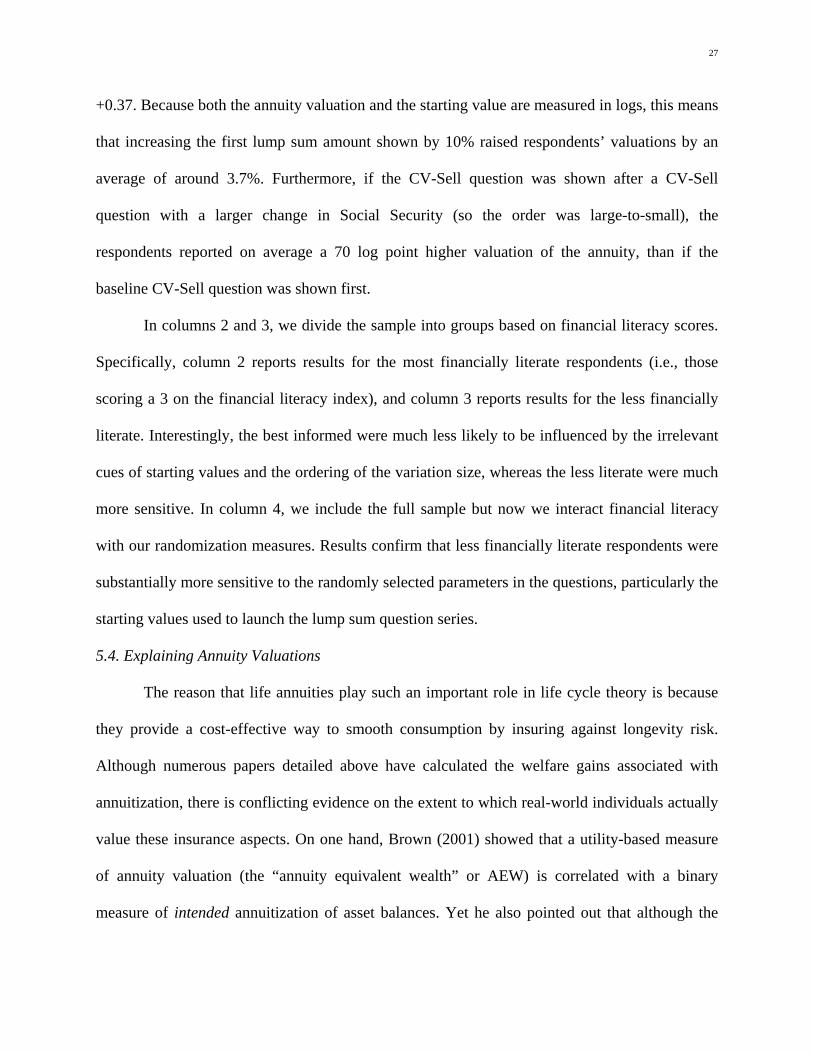
In columns 2 and 3, we divide the sample into groups based on financial literacy scores.
Specifically, column 2 reports results for the most financially literate respondents (i.e., those
scoring a 3 on the financial literacy index), and column 3 reports results for the less financially
literate. Interestingly, the best informed were much less likely to be influenced by the irrelevant
cues of starting values and the ordering of the variation size, whereas the less literate were much
more sensitive. In column 4, we include the full sample but now we interact financial literacy
with our randomization measures. Results confirm that less financially literate respondents were
substantially more sensitive to the randomly selected parameters in the questions, particularly the
starting values used to launch the lump sum question series.
5.4. Explaining Annuity Valuations
The reason that life annuities play such an important role in life cycle theory is because
they provide a cost-effective way to smooth consumption by insuring against longevity risk.
Although numerous papers detailed above have calculated the welfare gains associated with
annuitization, there is conflicting evidence on the extent to which real-world individuals actually
value these insurance aspects. On one hand, Brown (2001) showed that a utility-based measure
of annuity valuation (the “annuity equivalent wealth” or AEW) is correlated with a binary
measure of intended annuitization of asset balances. Yet he also pointed out that although the

28
variable was statistically significant, it did not fully account for the variation in the annuity
decision. Similar findings were documented in the Swiss system by Bütler and Teppa (2007). On
the other hand, Brown et al. (2008) suggested that because the U.S. retirement system is so
focused on wealth accumulation rather than retirement payouts, people have been conditioned to
think about annuities in simple financial terms rather than as insurance contracts providing
consumption-smoothing lifelong benefits. This is consistent with research showing that
individuals resort to simplified decision-making heuristics in the face of complex decisions
(Benartzi et al. 2011).
Accordingly, we expect that when individuals confront tradeoffs of the type presented in
our survey, they find it difficult to sort through the lifetime utility implications and instead resort
to thinking in simpler financial terms. To test this hypothesis, we run a regression of annuity
valuations against various determinants of annuity demand. Column 1 of Table 4 regresses the
average CV valuation against the actuarial value of the annuity offer presented (which varies by
cohort, age at annuitization, and sex; it also assumes a real interest rate of 3%); we also include
controls for age, age squared, sex, marital status, race and ethnicity. The actuarial value has a
coefficient of 1.02, suggesting that there is approximately a one-for-one correspondence between
the actuarial value of the annuity and the subjective value placed by the individual on the
annuity. Column 2 replaces the actuarial value with the AEW measure from Brown (2002). This
is the theoretical value of the annuity from a parameterized life-cycle model with variation
coming from mortality differences by age, sex, marital status (which determines whether it is a
single or joint life optimization), risk aversion, and interactions of these variables through the
utility-maximizing model. Here we find that the coefficient on this predicted annuity value in
column 2 is not significantly different from zero. In results not detailed here, when we include

29
both the actuarial value and the utility-based measure, we continue to find that the actuarial value
is approximately one and the utility-based measure is insignificant. In columns 3 and 4 we repeat
this analysis using a much larger set of control variables with very similar results.
Table 5 repeats the regressions from column 1 of Table 4 in rows 1-5, with the addition
of our subjective annuity valuations. Similarly, rows 6-10 repeat the column 4 regressions from
Table 4; rows 1-5 and 6-10 only differ in the number of controls included in the regressions. We
report the coefficient on the actuarial value of the annuity as well as the Root MSE and
regression R-squared (in the interests of space). In rows 1-5, we note that for all four ways of
eliciting annuity valuations, the coefficient on the actuarial value is approximately one
(specifically, we cannot reject that it is one and we can reject that it is zero). Rows 6-10 show
that the inclusion of more controls lowers the estimated coefficient of the log-actuarial value, but
we cannot reject the null that the true parameter equals one. Overall, we view these results as
being consistent with individuals using simpler financial decision rules (e.g., “how long will it
take me to breakeven?”) rather than taking into account the more complex consumption-
smoothing and insurance considerations.
A second conclusion from Table 5 is that the R-squared values are very low. That is, even
though subjective annuity valuations are significantly correlated with actuarial values, our ability
to explain the overall variation in the annuity decision is quite small. The R-squareds range from
a low of 0.025 for the EV-Sell measure including a limited number of controls, to a high of 0.118
for the CV-Sell measure with an extended set of controls. This is consistent with prior studies
(e.g., Brown 2008) that have also found it difficult to account for the observed variation in
annuitization decisions.

30
Table 6 reports coefficient estimates on the annuity valuation in sub-samples according to
respondent financial literacy. We have three such measures: (1) the financial literacy index used
above; (2) the degree of coherence in the EV-Sell and EV-Buy measures (which can then be used
as independent variables in the regression of CV measures); and (3) the respondent’s level of
education. We report the coefficients as well as the root mean squared error (MSE) for each
specification. Although the coefficients differ in the sub-groups, none of the coefficients differs
significantly between the most and least literate groups. Even more interesting is the magnitude
of the root MSE: this is much higher for less financially sophisticated individuals. Recalling that
our dependent variable is in logs, these differences are economically meaningful. For example,
the root mean square distance from the regression line for non-college graduates is nearly 0.3 log
points greater than for those with a college education. Thus it appears that the decisions made by
less financially sophisticated individuals are substantially noisier than for more sophisticated
individuals, a finding that is again consistent with a complexity explanation.
6. Discussion and Conclusions
This paper offers support for the hypothesis that many people find the annuitization
decision quite complex, and this complexity can help explain the observed low levels of annuity
purchase. Specifically, we find that consumers tend to value annuities less when given the
opportunity to buy more, but they value them more highly when given the opportunity to sell
annuities in exchange for lump sums. Because this finding holds even when no status quo option
is available, we believe that this finding is not driven by standard status quo or endowment effect
models. Rather, our results are consistent with individuals showing a strong preference for the
simpler, more understandable option (the lump sum), and only being willing to consider the more

31
complex option (the annuity) when it is an exceptionally good deal. This tendency is stronger
among those who are less financially sophisticated. We also show that complexity matters,
including the fact that people are sensitive to framing and starting values, and that the cross-
sectional variation in annuity values is correlated with simple financial valuations but not with
more complex annuity valuations.
Evidence that decision complexity could limit annuity demand has a number of important
implications for future retirement security research. First, such a finding may raise doubts about
whether consumers are able to make utility-maximizing choices when confronted with the
decision about whether to buy longevity protection in real-world situations. If individuals find
these decisions to be complex, this could help assess various policy interventions ranging from
providing better information, to changing the default option in the typical DC plan to partial
annuitization, or mandating some measure of compulsory annuitization. Naturally, the degree of
compulsory annuitization deemed optimal is also a first-order consideration in determining the
appropriate level of Social Security benefits in the U.S. and elsewhere.
Second, our findings imply that observers must be very careful when drawing
conclusions about individual welfare based on observed behavior (i.e., “revealed preference”)
when it comes to annuities, and quite possibly other complex financial products such as long-
term care insurance. For example, the fact that so few people annuitize their defined contribution
pension balances when given the opportunity to do so cannot be interpreted as conclusive
evidence that they do not value longevity protection.
In addition to advancing our academic understanding of consumer behavior in this area,
our results also have considerable policy relevance. The U.S. Social Security system is on a
fiscally unsustainable path that will require increasing revenue or curtailing benefit growth in the

32
not-too-distant future (Cogan and Mitchell 2003). As policymakers evaluate alternative
approaches to reform, it is important to understand how individuals actually value the system’s
mandatory old-age annuity payments, and how this perceived value is affected by the nature and
the framing of the trade-off presented. Nevertheless, we offer no road map as to whether which
people might be willing to pay to maintain the current system, nor can we pinpoint people’s
willingness to give up some portion of their annuity benefits in exchange for a lump sum. And
those who are more financially literate do have a more coherent approach to annuity valuation.
Our findings are also relevant to those concerned with state and local pension plan
underfunding in the U.S. For instance, these public plans are now grappling with how to reform
their defined benefit (DB) pensions to address underfunding problems (e.g., Novy-Marx and
Rauh 2011). Accordingly, there is an active discussion raging in policy circles regarding how to
measure annuities for defined contribution or 401(k) pension plans, with increasing attention
devoted to the role of payout annuities in such settings (c.f. Gale et al. 2008). In an aging world,
it is critical to understand why some people continue to be ill-protected against outliving their
retirement assets while others are not, and to find ways to strengthen markets for longevity
protection in the form of payout annuities.

33
References Agnew, Julie R., Lisa R. Anderson, Jeffrey R. Gerlach and Lisa R. Szykman. 2008. “Who Chooses
Annuities? An Experimental Investigation of the Role of Gender, Framing and Defaults.” American Economic Review. 98(2): 418-422.
Benartzi, Shlomo, Alessandro Previtero and Richard H. Thaler. 2011. “Annuitization Puzzles.” Journal of Economics Perspectives. 25(4): 143-64.
Benartzi, Shlomo and Richard H. Thaler. 2002. “How Much is Investor Autonomy Worth?” The Journal of Finance. 57(4): 1593 – 1616.
Bernheim, B. Douglas. 2002. “Taxation and Saving”. In Handbook of Public Economics. Eds Alan J. Auerbach and Martin Feldstein. New York: Elsevier. 1173-1249.
Beshears, John, James J. Choi, David Laibson, Brigitte C. Madrian. 2008. “How Are Preferences Revealed?” Journal of Public Economics. 92(8-9): 1787-1794.
Brown, Jeffrey R. 2001. “Private Pensions, Mortality Risk, and the Decision to Annuitize.” Journal of Public Economics. 82(1): 29–62.
Brown, Jeffrey R. 2008. “Understanding the Role of Annuities in Retirement Planning.” In Overcoming the Savings Slump: How to Increase the Effectiveness of Financial Education and Saving Programs. Ed. Annamaria Lusardi. Chicago: University of Chicago Press. 178 – 206.
Brown, Jeffrey R. 2009. “Automatic Lifetime Income as a Path to Retirement Security.” White paper for the American Council of Life Insurers. http://www.acli.com/Events/Documents/3f3ac12d2d004472906283563c87ee55Automatic_Lifetime_IncomePaper.pdf Last accessed 9/15/2011.
Brown, Jeffrey R., Marcus Casey, and Olivia S. Mitchell. 2008a. “Who Values the Social Security Annuity? Evidence from the Health and Retirement Study.” Unpublished manuscript.
Brown, Jeffrey R., Arie Kapteyn, and Olivia S. Mitchell. 2013. “Framing and Claiming: How Information-Framing Affects Expected Social Security Claiming Behavior.” Journal of Risk and Insurance. (forthcoming).
Brown, Jeffrey R., Jeffrey R. Kling, Sendhil Mullainathan and Marian Wrobel. 2008b. “Why Don’t People Insure Late Life Consumption? A Framing Explanation of the Under-Annuitization Puzzle.” American Economic Review. 98(2): 304-309.
Brown, Jeffrey R., Olivia S. Mitchell, and James M. Poterba. 2001. “The Role of Real Annuities and Indexed Bonds in an Individual Accounts Retirement Program.” In Risk Aspects of Investment-Based Social Security Reform. Eds. J. Campbell and M. Feldstein. Chicago: University of Chicago Press: 321–360.

34
Brown, Jeffrey R., Olivia S. Mitchell, and James M. Poterba. 2002. “Mortality Risk, Inflation Risk, and Annuity Products,” In Innovations in Retirement Financing. Eds. Olivia S. Mitchell, Zvi Bodie, Brett Hammond, and Steve Zeldes. Philadelphia: University of Pennsylvania Press: 175–197.
Brown, Jeffrey R., and James M. Poterba. 2000. “Joint Life Annuities and the Demand for Annuities by Married Couples.” Journal of Risk and Insurance 67(4): 527–553.
Bütler, Monika and Frederica Teppa. 2007. “The Choice between an Annuity and a Lump Sum: Results from Swiss Pension Funds.” Journal of Public Economics. 91(10): 1944-1966.
Cappelletti, Giuseppe, Giovanni Guazzarotti, and Pietro Tommasino. 2011. “What Determines Annuity Demand at Retirement?” Bank of Italy Temi di Discussione Working Paper No. 805.
Chalmers, John and Jonathan Reuter. 2012. “How Do Retirees Value Life Annuities? Evidence From Public Employees.” Review of Financial Studies. 25(8): 2601-2634..
Chai, Jingjing, Wolfram Horneff, Raimond Maurer, and Olivia S. Mitchell. 2011. “Optimal Portfolio Choice over the Life Cycle with Flexible Work, Endogenous Retirement, and Lifetime Payouts.” Review of Finance. 15(4): 875-907.
Choi, James, David Laibson and Brigitte C. Madrian. 2005. “Are Empowerment and Education Enough? Underdiversification in 401(k) Plans.” Brookings Papers on Economic Activity. 2: 151–198.
Cogan, John F. and Olivia S. Mitchell. 2003. “Perspectives from the President’s Commission on Social Security Reform.” Journal of Economic Perspectives. 17(2). Spring: 149–172.
Davidoff, Thomas, Jeffrey R. Brown, and Peter A. Diamond. 2005. “Annuities and Individual Welfare.” American Economic Review 95(5): 1573–1590.
Dushi, Irena and Anthony Webb. 2006. “Rethinking the Sources of Adverse Selection in the Annuity Market.” In Competitive Failures in Insurance Markets: Theory and Policy Implications. Eds. Pierre Andre Chiappori and Christian Gollier. Cambridge: MIT Press: 185-212.
Gale, William G., J. Mark Iwry, David C. John and Lina Walker. 2008. Increasing Annuitization of 401(k) Plans with Automatic Trial Income. Retirement Security Project Report. Washington, D.C.: Brookings Institution.
Greenwald, Mathew, Arie Kapteyn, Olivia S. Mitchell, and Lisa Schneider. 2010. “What Do People Know about Social Security?” Financial Literacy Consortium Report to the SSA, September.
Horneff, Wolfram, Raimond Maurer, Olivia S. Mitchell, and Ivica Dus. 2007. “Following the Rules: Integrating Asset Allocation and Annuitization in Retirement Portfolios.” Insurance: Mathematics and Economics. 42(1): 396-408.
Horneff, Wolfram, Raimond Maurer, Olivia S. Mitchell, and Michael Stamos. 2009. “Asset Allocation and Location over the Life Cycle with Survival-Contingent Payouts.” Journal of Banking and Finance. 33(9): 1688-1699.

35
Horneff, Wolfram J. Raimond H. Maurer, Olivia S. Mitchell, and Michael Z. Stamos. 2010. “Variable Payout Annuities and Dynamic Portfolio Choice in Retirement.” Journal of Pension Economics and Finance. 9(2): 163-183.
Hurd, Michael and Stan Panis. 2006. "The Choice to Cash out Pension Rights at Job Change or Retirement." Journal of Public Economics. 90(12): 2213-2227.
Inkmann, Joachim, Paula Lopes, and A. Michaelides. 2011. “How Deep is the Annuity Market Participation Puzzle?” Review of Financial Studies. 24(1): 279-319.
Kahneman, Daniel, and Amos Tversky. (1981). “The Framing of Decisions and the Psychology of Choice.” Science. 211(4481): 453-458.
Kahneman, Daniel, Knetsch, J. L. and Thaler, R. H. 1991. “Anomalies: The Endowment Effect, Loss Aversion, and Status Quo Bias.” Journal of Economic Perspectives. 5(1): 193-206
Kilgour, John G. 2006. “Public Sector Pension Plans: Defined Benefit Versus Defined Contribution.” Compensation Benefits Review. 38(1): 20-28.
Kling, Catherine L., Daniel J. Phaneuf, and Jinhua Zhao. 2012. "From Exxon to BP: Has Some Number Become Better than No Number?" Journal of Economic Perspectives. 26(4): 3–26.
Koijen, Ralph S.J., Nijman, Theo E. and Werker, Bas J.M. 2011. "Optimal Annuity Risk Management." Review of Finance. 15(4): 799-833.
Kotlikoff, Laurence J., and Avia Spivak. 1981. “The Family as an Incomplete Annuities Market.” Journal of Political Economy. 89(2): 372–391.
Liebman, Jeffrey B. and Erzo F.P. Luttmer. 2011. “The Perception of Social Security Incentives for Labor Supply and Retirement: The Median Voter Knows More Than You’d Think.” Unpublished Manuscript, Dartmouth College.
Lockwood, Lee. 2011. "Bequest Motives and the Annuity Puzzle." Review of Economic Dynamics.15(2): 226-243.
Lusardi, Annamaria and Olivia S. Mitchell. 2007. “Baby Boomer Retirement Security: The Roles of Planning, Financial Literacy, and Housing Wealth.” Journal of Monetary Economics. 54(1): 205-224.
Maurer, Raimond, Olivia S. Mitchell, Ralph Rogalla, and Vasily Kartashov. 2013. “Lifecycle Portfolio Choice with Stochastic and Systematic Longevity Risk, and Variable Investment-Linked Deferred Annuities.” Journal of Risk and Insurance. Forthcoming.
Milevsky, Moshe and Virginia R. Young. 2007. “Annuitization and Asset Allocation.” Journal of Economic Dynamics and Control. 31(9): 3138-3177.
Mitchell, Olivia S., James M. Poterba, Mark J. Warshawsky, and Jeffrey R. Brown. 1999. “New Evidence on the Money’s Worth of Individual Annuities.” American Economic Review 89(5): 1299–1318.

36
Mitchell, Olivia S., John Piggott, and Noriyuke Takayama, eds. 2011. Securing Lifelong Retirement Income. Oxford: Oxford University Press.
Modigliani, Franco. 1988. "The Role of Intergenerational Transfers and Life-Cycle Saving in the Accumulation of Wealth." Journal of Economic Perspectives. 2(2): 15-40.
Novy-Marx, Robert and Joshua Rauh. 2011. “The Liabilities and Risks of State-Sponsored Pension Plans.” Journal of Economic Perspectives. 23(4): 191-210.
Peijnenburg, Kim, Theo Nijman and Bas Werker. 2010a. “Optimal Annuitization with Incomplete Annuity Markets and Background Risk during Retirement.” Netspar Discussion Paper.
Peijnenburg, Kim, Theo Nijman, and Bas J.M. Werker. 2010b. "Health Cost Risk and Optimal Retirement Provision: A Simple Rule for Annuity Demand." Wharton School Pension Research Council Working Paper No. WPS 2010-08.
Poterba, James, Steve Venti, and David Wise. 2011. “The Drawdown of Personal Retirement Assets.” NBER Working Paper 16675.
Reichling, Felix and Kent Smettters. 2012. “Optimal Annuitization with Stochastic Mortality Probabilities.” BYU Computational Public Economic Conference Presentation, December.
Samuelson, William and Richard J. Zeckhauser. 1988. “Status-quo Bias in Decision Making.” Journal of Risk and Uncertainty. 1: 7-59.
Shepard, Mark. 2011. “Social Security Claiming and the Life Cycle Model.” Unpublished Manuscript, Harvard University.
Simon, Herbert A. 1947. Administrative Behavior, a Study of Decision-Making Processes in Administrative Organization. New York: Macmillan.
Sinclair, Sven H. and Kent A. Smetters. 2004. “Health Shocks and the Demand for Annuities.” Technical
Paper Series; Congressional Budget Office. Washington, DC: GPO, July Turra, Cassio and Olivia S. Mitchell. 2008. “The Impact of Health Status and Out-of-Pocket Medical
Expenditures on Annuity Valuation.” In Recalibrating Retirement Spending and Saving. Eds. John Ameriks and Olivia S. Mitchell. Oxford University Press: 227-250.
Warner, John T., and Saul Pleeter. 2001. “The Personal Discount Rate: Evidence from Military
Downsizing Programs.” American Economic Review 91(1): 33-53.
Wayland, Michael. 2012. “GM Pensions: 13,200 White Collar Retirees Taking Buyouts Makes Sense, Analysts Say.” http://www.mlive.com/auto/index.ssf/2012/11/gm_pensions_12600_white-collar.html.
Yaari, Menachim. 1965. "Uncertain Lifetime, Life Insurance, and the Theory of the Consumer." Review of Economic Studies. 32(2): 137-150.

37
Figure 1: CDF of "CV-Sell" for $100/mo Additional Social Security Annuity

38
Figure 2: CDF of Willingness to Buy versus Willingness to Sell a $100/mo Social Security Annuity

39
Figure 3. CDF of Equivalent Variation of a $100/mo Social Security Annuity
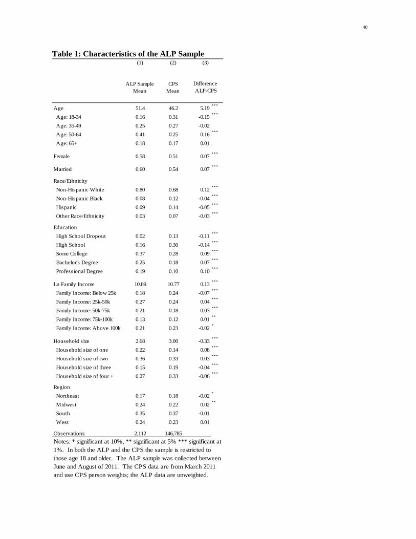
40
Table 1: Characteristics of the ALP Sample
(1) (2)
ALP SampleMean
CPSMean
Age 51.4 46.2 5.19***
Age: 18-34 0.16 0.31 -0.15***
Age: 35-49 0.25 0.27 -0.02
Age: 50-64 0.41 0.25 0.16***
Age: 65+ 0.18 0.17 0.01
Female 0.58 0.51 0.07***
Married 0.60 0.54 0.07***
Race/Ethnicity
Non-Hispanic White 0.80 0.68 0.12***
Non-Hispanic Black 0.08 0.12 -0.04***
Hispanic 0.09 0.14 -0.05***
Other Race/Ethnicity 0.03 0.07 -0.03***
Education
High School Dropout 0.02 0.13 -0.11***
High School 0.16 0.30 -0.14***
Some College 0.37 0.28 0.09***
Bachelor's Degree 0.25 0.18 0.07***
Professional Degree 0.19 0.10 0.10***
Ln Family Income 10.89 10.77 0.13***
Family Income: Below 25k 0.18 0.24 -0.07***
Family Income: 25k-50k 0.27 0.24 0.04***
Family Income: 50k-75k 0.21 0.18 0.03***
Family Income: 75k-100k 0.13 0.12 0.01**
Family Income: Above 100k 0.21 0.23 -0.02*
Household size 2.68 3.00 -0.33***
Household size of one 0.22 0.14 0.08***
Household size of two 0.36 0.33 0.03***
Household size of three 0.15 0.19 -0.04***
Household size of four + 0.27 0.33 -0.06***
Region
Northeast 0.17 0.18 -0.02*
Midwest 0.24 0.22 0.02**
South 0.35 0.37 -0.01
West 0.24 0.23 0.01
Observations 2,112 146,785
Notes: * significant at 10%, ** significant at 5% *** significant at 1%. In both the ALP and the CPS the sample is restricted to those age 18 and older. The ALP sample was collected between June and August of 2011. The CPS data are from March 2011 and use CPS person weights; the ALP data are unweighted.
Difference ALP-CPS
(3)
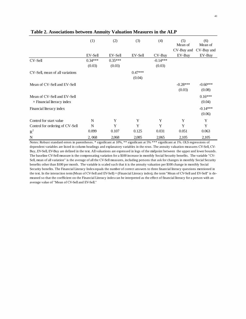
41
Table 2. Associations between Annuity Valuation Measures in the ALP
CV-Sell
CV-Sell, mean of all variations
Mean of CV-Sell and EV-Sell
Mean of CV-Sell and EV-Sell × Financial literacy index
Financial literacy index
Control for start valueControl for ordering of CV-Sell
R2
N
0.35***(0.03)
0.47***(0.04)
-0.14***(0.03)
-0.28*** -0.60***(0.08)
0.16***(0.04)
-0.14***(0.06)
(0.03)
Y Y Y Y
(2)Mean of
CV-Buy and EV-Buy
(5)
CV-Buy
(4)
EV-Sell
(3)
Y
0.34***(0.03)
N
Mean of CV-Buy and
EV-Buy
(6)
Notes: Robust standard errors in parentheses. * significant at 10%, ** significant at 5% *** significant at 1%. OLS regressions of dependent variables are listed in column headings and explanatory variables in the rows. The annuity valuation measures CV-Sell, CV-Buy, EV-Sell, EV-Buy are defined in the text. All valuations are expressed in logs of the midpoint between the upper and lower bounds. The baseline CV-Sell measure is the compensating variation for a $100 increase in monthly Social Security benefits. The variable "CV-Sell, mean of all variation" is the average of all the CV-Sell measures, including persons that ask for changes in monthly Social Security benefits other than $100 per month. The variable is scaled such that it is the annuity valuation per $100 change in monthly Social Security benefits. The Financial Literacy Index equals the number of correct answers to three financial literacy questions mentioned in the text. In the interaction term (Mean of CV-Sell and EV-Sell) × (Financial Literacy index), the term "Mean of CV-Sell and EV-Sell" is de-meaned so that the coefficient on the Financial Literacy index can be interpreted as the effect of financial literacy for a person with an average value of "Mean of CV-Sell and EV-Sell."
N
0.099
2, 068
Y Y Y Y Y
0.107 0.125 0.031 0.051 0.063
2,068 2,085 2,065 2,105 2,105
EV-Sell
(1)
EV-Sell

42
Table 3: Effect of Randomizations and Interactions with Financial Literacy
VariablesLog of starting value
Asked after larger version
Asked in wave 1
Lump sum option shown last
Log of starting value × Financial literacy index
Asked after larger version × Financial literacy index
Asked in wave 1 × Financial literacy index
Lump sum option shown last × Financial literacy index
Financial literacy index
R2
N
0.18 0.48*** 0.98***
0.57*** 0.75*** 0.74***
(0.11) (0.10) (0.25)
(0.05)
-0.28***
-0.14***
0.70***(0.07) (0.10) (0.08) (0.22)
0.04(0.07)
-0.07(0.10)
0.11(0.09)
0.31(0.22)
0.05(0.22)
(0.11)
-0.03(0.09)
-0.12(0.09)
0.02(0.09)
0.09(0.07)
0.01(0.10)
0.12(0.09)
(0.07)
Dependent Variable: CV-Sell (in logs)
Entire sample
(1) (2)
Most financially literate
(3)
Least financially literate
(4)
Entire sample
Notes: Robust standard errors in parentheses. * significant at 10%, ** significant at 5% *** significant at 1%. Each column contains an OLS regression of the baseline CV-Sell measure on the explanatory variables listed in the rows. The baseline CV-Sell measure is the compensating variation for a $100 increase in monthly Social Security benefits, expressed in logs of the midpoint between the upper and lower bounds. The starting value for the annuity valuation was randomized at $10,000, $20,000, or $30,000. "Asked after larger version" equals one if the baseline CV-Sell measure was asked after a CV-Sell question where Social Security benefits were varied by more than $100. Whether this occured was randomized. "Asked in wave 1" is a dummy variable that equals one if the CV-Sell question was asked in the first wave and "Lump sum option shown last" is a dummy variable that equals one if the option involving the lump sum amount was shown after the alternative option. Both dummy variables were randomized. The Financial Literacy index equals the number of correct answers to three financial literacy questions, and those getting all three questions correct are categorized as most financially literate. All variables interacted with the financial literacy index are de-meaned so that the coefficient on the financial literacy index can be interpreted as the effect of the financial literacy index when the interaction variables are at their sample means.
0.062 0.043 0.074 0.072
2,090 726 1,364 2,090
0.37***

43
Table 4: Explaining Annuity Valuations Dep. Variable: Mean of CV-Sell and CV-Buy
(in logs) Explanatory Variables (1) (2) (3) (4) Log actuarial value 1.02*** 0.84***
(0.25) (0.26) Log predicted annuity value 0.04 0.18
(0.04) (0.13) Age -0.05*** -0.02 -0.04** -0.01
(0.01) (0.01) (0.02) (0.01) Age squared/100 0.06*** 0.02 0.04*** 0.01
(0.02) (0.01) (0.02) (0.01) Female -0.08 0.01 -0.03 0.01
(0.06) (0.05) (0.06) (0.06) Married 0.05 0.04 0.08 0.13*
(0.06) (0.06) (0.06) (0.07) Black 0.05 0.08 0.03 0.04
(0.12) (0.12) (0.12) (0.12) Hispanic 0.34*** 0.36*** 1.02*** 0.32***
(0.11) (0.11) (0.12) (0.12) Other -0.08 -0.08 -0.08 -0.09
(0.13) (0.13) (0.12) (0.13) Education Index, 1-5 scale -0.03 -0.03
(0.03) (0.03) Log family income 0.03 0.02
(0.04) (0.04) Owns an annuity -0.07 -0.04
(0.06) (0.06) Owns home -0.16* -0.16***
(0.08) (0.08) Log financial wealth 0.01 -0.01
(0.02) (0.03) Self-reported health index, 1-5 scale -0.03 -0.03
(0.03) (0.03) Ever had kids -0.03 -0.04
(0.06) (0.06) Risk aversion (standardized) 0.02 0.02
(0.03) (0.03) Precaution (standardized) -0.07** -0.07**
(0.03) (0.03) Expects returns greater than 3% p.a. 0.10* 0.10*
(0.06) (0.06)

44
Confident SS will pay promised benefits, 1-4 scale 1.02*** 0.14*** (0.03) (0.03)
Controls for Exper. Var. Yes Yes Yes Yes R-squared 0.060 0.053 0.080 0.076
Number of observations 2065 2065 2065 2065 Notes: Robust standard errors between parentheses. * significant at 10%, ** significant at 5% *** significant at 1%. Each column contains an OLS regression of annuity valuation (CV-Sell) on the explanatory variables listed in the rows. CV-Sell is the compensating variation for a $100 increase in monthly Social Security benefits, and is expressed in logs of the midpoint between in the upper and lower bound. All regressions also include controls for missing values of explanatory variables and controls for experimental variation, namely: log of starting value, asked after larger version, asked in wave 1, lump sum option shown last. The log predicted annuity value is the CV-Sell is found by solving the lifecycle dynamic programming problem for a household that matches the respondent on age, gender, marital status, spousal age (if married), start date of the annuity, financial wealth, existing annuity wealth, and coefficient of risk aversion. See text for details. The education index equals 1 for high school dropouts, 2 for high school graduates, 3 for some college, 4 for bachelor's degree, and 5 for professional degree.

45
Table 5: Robustness of the Predictive Power of Actuarial Value (1) (2) (3) (4) (5) (6) (7)
Dependent Variable
Coefficient on log actuarial value
p-value on coefficient=1 Controls Root MSE
R-squared N
1. Mean of CV-Sell
and CV-Buy
1.02*** 0.940 Basic 1.187 0.060 2065
(0.25)
2. CV-Sell 1.05*** 0.883 Basic 1.496 0.087 2090
(0.34)
3. CV-Buy 0.98** 0.955 Basic 2.026 0.037 2086
(0.44)
4. EV-Sell 0.74** 0.492 Basic 1.692 0.025 2089
(0.37)
5. EV-Buy 0.84* 0.734 Basic 2.140 0.033 2082
(0.48)
6. Mean of CV-Sell
and CV-Buy
0.84*** 0.536 Extensive 1.180 0.080 2065
(0.26)
7. CV-Sell 0.63* 0.281 Extensive 1.478 0.118 2090
(0.34)
8. CV-Buy 1.03** 0.945 Extensive 2.012 0.061 2086
(0.45)
9. EV-Sell 0.36 0.095 Extensive 1.680 0.049 2089
(0.38)
10. EV-Buy 0.96* 0.930 Extensive 2.129 0.053 2082
(0.49) Notes: Robust standard errors in parentheses. * significant at 10%, ** significant at 5% *** significant at 1%. Each row contains an OLS regression of the log annuity valuation measure listed in column 1 on the log actuarial value and additional controls. The annuity valuation measures CV-Sell, CV-Buy, EV-Sell, EV-Buy are defined in the text. All valuations are expressed in logs of the midpoint between the upper and lower bounds. Additional controls in rows 1-5 are those in specification 1 of Table 4 whereas the additional controls in rows 6 through 10 are those in specification 4 of Table 3. Rows 1 and 6 replicate columns 1 and 3 of Table 4, respectively.

46
Table 6: Predictive Power of Actuarial Value by Measures of Financial Sophistication
Notes: Robust standard errors in parentheses. * significant at 10%, ** significant at 5% *** significant at 1%. Here we estimate specification 1 of Table 4 by subsample. Each row contains an OLS regression of the log annuity valuation (mean of CV-Sell and CV-Buy) on the log actuarial value and additional controls. Additional controls are those in specification 1 of Table 4. Financial literacy is defined by the number of correct answers to three financial literacy questions, and those getting all three questions correct are categorized as most financially literate. EV coherence measures the similarity between the EV-Sell and the EV-Buy valuation. Those for whom the log difference between EV-Sell and EV-Buy falls in the bottom tercile are categorized as most EV coherent.
(1) (2) (3) (4) (5) (6) (7)Dependent variable: Mean of CV-Sell and CV-Buy
Coefficient on log actuarial
p-value on coefficient Controls Root MSE R-squared N
1. Sample split by financial literacyMost financially literate 0.93** 0.854 Basic 1.085 0.050 723
(0.40)Least financially literate 0.99*** 0.969 Basic 1.239 0.069 1342
(0.33)p-value on test that coefficients are the same [0.914]
2. Sample split by EV coherenceMost EV coherent 0.40 0.068 Basic 0.812 0.137 680
(0.33)Least EV Coherent 1.28*** 0.397 Basic 1.327 0.056 1385
(0.33)p-value on test that coefficients are the same [0.058]
3. Sample split by educational attainmentBachelor's degree or more 1.47*** 0.141 Basic 1.023 0.084 916
(0.32)Some college or less 0.61 0.308 Basic 1.303 0.055 1149
(0.38)p-value on test that coefficients are the same [0.056]

47
Data Appendix: The Rand American Life Panel
Sample Construction
Our survey was conducted in the RAND American Life Panel (ALP). The ALP consists of a panel of U.S. households that regularly takes surveys over the Internet. An advantage relative to most other Internet panels is that the respondents to the ALP need not have Internet when they get recruited (as is described in more detail below) and thus can be based on a probability sample of the US population.20 This is in contrast with so-called convenience Internet samples, where respondents are volunteers who already have Internet and for example respond to banners placed on frequently visited web-sites, in which they are invited to do surveys and earn money doing it. The problem with convenience Internet samples is that their statistical properties are unknown. There is a fairly extensive literature comparing probability Internet samples like the ALP and convenience Internet samples or trying to establish if convenience samples can somehow be made population representative by reweighting.
For instance, Chang and Krosnick (2009) simultaneously administered the same questionnaire (on politics) to an RDD (random digit dialing) telephone sample, an Internet probability sample, and a non-probability sample of volunteers who do Internet surveys for money. They found that the telephone sample has most random measurement error, while the non-probability sample has the least. At the same time, the latter sample exhibits most bias (also after reweighting), so that it produces the most accurate self-reports from the most biased sample. The probability Internet sample exhibited more random measurement error than the non-probability sample (but less than the telephone sample) and less bias than the non-probability Internet sample. On balance, the probability Internet sample produced the most accurate results. Yeager et al. (2009) conducted a follow-up study comparing one probability Internet sample, one RDD telephone sample, and seven non-probability Internet samples and a wider array of outcomes. Their conclusions are the same: Both the telephone sample and the probability Internet sample show the least bias; reweighting the non-probability samples does not help (for some outcomes, the bias gets worse; for others, better). They also found that response rates do not appear critical for bias. Even with relatively low response rates, the probability samples yield unbiased estimates. It is not clear a priori why non-probability samples do so much worse. As they note, it appears that there are some fundamental differences between Internet users and non-Internet users that cannot be redressed by reweighting. Indeed, Couper et al. (2007) and Schonlau et al. (2009) show weighting and matching do not eliminate differences between estimates based on samples of respondents with and without Internet access. Several other studies point at equally mixed results, including Vehovar et al. (1999); Duffy et al., (2005); Malhotra and Krosnick (2007), Taylor (2000), Loosveldt and Sonck (2008).
ALP respondents have been recruited in one of four ways. Most were recruited from respondents age 18+ to the Monthly Survey (MS) of the University of Michigan’s Survey Research Center (SRC). The MS is the leading consumer sentiment survey that incorporates the long-standing Survey of Consumer Attitudes and produces, among others, the widely used Index of Consumer Expectations. Each month, the MS interviews approximately 500 households, of
20 Other probability Internet surveys include the Knowledge Networks panel in the U.S. (http://www.knowledgenetworks.com/knpanel/index.html), and the CentERpanel and LISS panel in the Netherlands: (http://www.centerdata.nl/en/centerpanel and http://www.centerdata.nl/en/MESS ). Of these the CentERpanel is the oldest (founded in 1991).

48
which 300 households are a random-digit-dial (RDD) sample and 200 are re-interviewed from the RDD sample surveyed six months previously. Until August 2008, SRC screened MS respondents by asking them if they would be willing to participate in a long-term research project (with approximate response categories “no, certainly not,” “probably not,” “maybe,” “probably,” “yes, definitely”). If the response category is not “no, certainly not,” respondents were told that the University of Michigan is undertaking a joint project with RAND. They were asked if they would object to SRC sharing their information about them with RAND so that they could be contacted later and asked if they would be willing to actually participate in an Internet survey. Respondents who do not have Internet were told that RAND will provide them with free Internet. Many MS-respondents are interviewed twice. At the end of the second interview, an attempt was made to convert respondents who refused in the first round. This attempt includes the mention of the fact that participation in follow-up research carries a reward of $20 for each half-hour interview. Respondents from the Michigan monthly survey without Internet were provided with so-called WebTVs (http://www.webtv.com/pc/), which allows them to access the Internet using their television and a telephone line. The technology allows respondents who lacked Internet access to participate in the panel and furthermore use the WebTVs for browsing the Internet or email. The ALP has also recruited respondents through a snowball sample (respondents suggesting friends or acquaintances who might also want to participate), but we do not use any respondents recruited through the snowball sample in our paper. A new group of respondents (approximately 500) has been recruited after participating in the National Survey Project, created at Stanford University with SRBI. This sample was recruited in person, and at the end of their one-year participation, they were asked whether they were interested in joining the RAND American Life Panel. Most of these respondents were given a laptop and broadband Internet access. Recently, the American Life Panel has begun recruiting based on a random mail and telephone sample using the Dillman et al. method (2008) with the goal to achieve 5,000 active panel members, including a 1,000 person Spanish language subsample. If these new participants did not yet have Internet access, they are also provided with a laptop and broadband Internet access.
Calculation of Social Security Benefits
For most ALP respondents, we have previously estimated monthly Social Security benefits (described in Brown et al., 2013). To do so, we took respondents through a fairly detailed set of questions asking about years in which they had labor earnings and an approximation of earnings in those years. We then fed these earnings through a benefit calculator provided by SSA to calculate the individual’s “Primary Insurance Amount” (PIA) which is equivalent to the benefit the individual would receive if he were to retire at his normal retirement age. Next we applied SSA’s actuarial adjustment for earlier or later claiming. We also asked respondents if the estimated benefit amount seemed reasonable to them, and we gave them an opportunity to change this estimate if they believed it was not a good approximation. All subsequent lump sum and annuity questions then pivot off this estimated monthly Social Security benefit amount.
For the few respondents who indicated they did not expect to receive a benefit (nor did they expect one from a living or deceased spouse), we imputed ‘standard monthly benefit amounts’ based on age, sex, and educational levels. We then ask the respondent to assume, for the purposes of the questions to follow, that he or she would receive this benefit, as follows:

49
Even though we understand that you are not eligible to receive Social Security benefits, we would like to ask you to complete this survey assuming you would be eligible. In other words, please answer in this survey what you would have done or chosen if you would be eligible for Social Security benefits.
Appendix References Brown, J. R., A. Kapteyn, and O. S. Mitchell. 2013. “Framing and Claiming: How Information-Framing
Affects Expected Social Security Claiming Behavior.” Journal of Risk and Insurance. (forthcoming).
Chang, L. and J.A. Krosnick. 2009. “National Surveys via RDD Telephone Interviewing versus the Internet: Comparing Sample Representativeness and Response Quality.” Public Opinion Quarterly, 73: 641-648.
Couper, M.P., A. Kapteyn, M. Schonlau, and J. Winter. 2007. “Noncoverage and Nonresponse in an Internet Survey.” Social Science Research. 36(1):131-148.
Dillman, D.A., J.D Smyth, and L.M. Christian. 2008. Internet, Mail, and Mixed-Mode Surveys: The Tailored Design Method, 3rd edition. Hoboken, NJ: Wiley.
Duffy, B., K. Smith, G. Terhanian, and J. Bremer. 2005. “Comparing Data from Online and Face-to-face Surveys.” International Journal of Market Research, 47: 615–639.
Lichtenstein, Sarah, and Paul Slovic. 1971. “Reversals of Preferences between Bids and Choices in Gambling Decisions.” Journal of Experimental Psychology. 89: 46-55.
Lichtenstein, Sarah and Paul Slovic. 1973. “Response-Induced Reversals of Preference in Gambling: An Extended Replication in Las Vegas.” Journal of Experimental Psychology. 010: 16-20.
Loosveldt, G. and N. Sonck. 2008. “An Evaluation of the Weighting procedures for an Online Access Panel Survey/” Survey Research Methods. 2: 93–105.
Malhotra, N. and J.A. Krosnick. 2007. “The Effect of Survey Mode and Sampling on Inferences about Political Attitudes and Behavior: Comparing the 2000 and 2004 ANES to Internet Surveys with Non-probability Samples.” Political Analysis. 15: 286–323.
Schonlau, M., A. van Soest, A. Kapteyn, and M. Couper. 2009. “Selection Bias in Web Surveys and the Use of Propensity Scores.” Sociological Methods and Research. 37: 291-318.
Taylor, H. 2000. “Does Internet Research Work? Comparing Online Survey Results with Telephone Surveys.” International Journal of Market Research. 42(1): 51–63.
Vehovar, V., Z. Batagelj, and K. Lozar Manfreda. 1999. “Web surveys: Can the weighting solve the problem?” Proceedings of the Survey Research Methods Section. American Statistical Association: 962–967.
Yeager, D.S., J.A. Krosnick, L. Chang, H.S. Javitz, M.S. Levindusky, A. Simpser, and R. Wang. 2009. “Comparing the Accuracy of RDD Telephone Surveys and Internet Surveys Conducted with Probability and Non-Probability Samples.” Working paper, Stanford University.
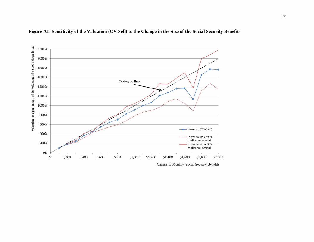
50
Figure A1: Sensitivity of the Valuation (CV-Sell) to the Change in the Size of the Social Security Benefits


![Efficient Annuitization: Optimal Strategies for Hedging ...€¦ · Efficient Annuitization: Optimal Strategies for Hedging Mortality Risk 1 Introduction Yaari [1965] theorized that](https://static.fdocuments.net/doc/165x107/5eac2e09a3ab5b4fad4f2f31/efficient-annuitization-optimal-strategies-for-hedging-efficient-annuitization.jpg)