Complex Analysis: A Brief Tour into Higher Dimensions · mathematics major in calculus of functions...

Complex Analysis: A Brief Tour into Higher Dimensions

R. Michael Range

1. INTRODUCTION. Why is it that most graduate students of mathematics (and many undergraduates as well) are exposed to complex analysis in one variable, yet only a small minority of students or, for that matter, professional mathematicians ever learn even the most basic corresponding theory in several variables? Think about it another way: Could anyone seriously argue that it might be sufficient to train a mathematics major in calculus of functions of one real variable without expecting him or her to learn at least something about partial derivatives, multiple integrals, and some higher dimensional version of the Fundamental Theorem of Calculus? Of course not, the real world is not one-dimensional! But neither is the complex world: witness classical applications of complex analysis to quantum field theory, more recent uses in twistor and gravitation theory, and the latest developments in string the-

ory! Multidimensional complex analysis is an indispensable tool in moder theoretical

physics. (See, for example, Green, Schwarz, and Witten [6], Manin [12], Henkin and Novikov [9].)

Aside from questions of applicability, shouldn't the pure mathematician's mind wonder about the restriction to functions of only one complex variable? It should not

surprise anyone that there is a natural extension of complex analysis to the multivariable setting. What is surprising is the many new and intriguing phenomena that appear when one considers more than one variable. Indeed, these phenomena presented ma-

jor challenges to any straightforward generalization of familiar theorems. Amazing progress was made in the 1940s and 1950s, when the area was enriched by new and

powerful tools such as coherent analytic sheaves and their cohomology theory. Yet for decades these apparently quite abstract techniques constituted a formidable barrier that deterred analysts from exploring this territory unless they were committed to a research career in multidimensional complex analysis. Fortunately, many of the technical hardships of the pioneering days can now be overcome with much less effort by approaching the subject along different routes.

The purpose of this article is to lead you, as painlessly as possible, on a tour through some of the foundations of complex analysis in several variables, and to take you to some vantage points from which we can enjoy some of the fascinating sights that remain hidden from us as long as we restrict ourselves to the complex plane. Along the way, we shall encounter a few of the unexpected higher dimensional phenomena and explore fundamental new concepts, always trying to gain an understanding of the underlying difficulties. Good walking shoes (i.e., an elementary introduction to basic complex analysis in one variable, and standard multivariable real calculus) are all the equipment that is needed, no technical gear or skills will be required. I will be rewarded if, at the end of our hike, many of you will recommend this tour to friends and colleagues. Perhaps a few of you will be sufficiently intrigued and challenged that you will pick up one of the excellent books that are available to guide you through more advanced terrain in order to reach the "high peaks" of the subject.

2. PRELIMINARIES. Complex Euclidean space C" = {z = (z, ... z) : zj E Cl is a complex vector space of dimension n over C. The Euclidean norm Izl of z in C"

COMPLEX ANALYSIS February 2003] 89

is defined by (.j Izl2)1/2. The familiar identification of C with R2 extends to a natural identification of C" with RI2, thereby giving immediate meaning to all concepts familiar from multivariable real analysis. A continuous function f : U -* C on an open set U in C" is said to be holomorphic on U if f is holomorphic in each variable separately, that is, if it satisfies the Cauchy-Riemann equation af/7zj = 0 on U in each variable zj, j = 1, ..., n.l For the sake of completeness, let us recall the familiar

partial differential operators

a 1 to ._ A a 1-ay t ,_ az =2 ax ay az 2 iax yay

where z = x + iy. In the multidimensional setting, these operators extend in the obvious way to each variable zj for j = 1, ..., n. The space of holomorphic functions on U is denoted by O(U). Just as in dimension one, standard local properties of holomor-

phic functions are most easily obtained by means of an integral representation formula, one that results from a straightforward iteration of the one variable Cauchy integral formula for discs, as follows. To simplify notation, we consider only the case n = 2; this will suffice to illustrate the main idea. For a = (al, a2) in C2 and r = (rl, r2) with rj > 0, the product of two discs P = P(a, r) = {z: Izj - aj I < rj, j = 1, 2} (a bidisc, or polydisc in the more general higher dimensional setting) is an open neighborhood of a. Suppose that f is holomorphic in a neighborhood of the closure P of P. With zl satisfying Izl - al < rl fixed, apply the Cauchy intergral formula in the second variable to the disc {Z2 : Iz2 - a2! < r2} to obtain

f (z, z2)= f (Z, 2) d2 27i J 2 - Z2

1 2-a2 =r2

Under the integral sign apply the Cauchy integral formula in the first variable, now keeping 22 fixed. Since f is continuous, we may replace the resulting iterated integral with a double integral over the distinguished boundary boP of P-defined by boP = {z : zj - aj = rj, j = 1, 2} (which is a product of circles, i.e., a torus)-to obtain the Cauchy integral formula for a bidisc:

f(z) = 1 f (1,?2)dl d' 2

(2ri)2 (i - Z1)('2 - Z2) boP

for z = (zl,Z2) in P. Standard analysis arguments now tell us that partial derivatives of f can be calcu-

lated by differentiating under the integral sign, that f belongs to the class C??(P), that every complex partial derivative D'f = alalflazl1az22 of f is again holomorphic, and so on. Similarly, one obtains the Taylor series expansion

D(~'~2) fD(a) f (Z) '= D , 2 ) (Z - l)Vi (2 a2)

2

vl, v2=0

for each z in P, with absolute convergence (hence convergence independent of the order of summation!) that is uniform on each compact subset of P.

In fact, the continuity hypothesis is not needed. Complex differentiability in each variable separately on U already implies continuity on the part of f, hence ensures that f is holomorphic as defined here. This deep and surprising result, which has no analog in real analysis, was proved by F. Hartogs in 1906.

0? THE MATHEMATICAL ASSOCIATION OF AMERICA [Monthly 110 90

Based on these local results, proofs of other fundamental facts are readily extended from one variable to several variables. In particular, compact convergence (meaning uniform convergence on each compact subset of an open set) of a sequence (or series) of holomorphic functions implies that the limit (respectively, sum) is again holomorphic, and that differentiation can be interchanged with the limit process. The Maximum Principle and Montel's theorem remain valid, and the identity theorem holds in the following form: if f belongs to O(U) and U is connected and if f = 0 on a nonempty open subset V of U, then f -0 on U. A map F = (fi,..., fm) : U -- Cm is said to be holomorphic if each component fi is holomorphic. The composition of holomorphic maps is holomorphic. If F is holomorphic, its derivative F' is a complex linear map represented by the m x n (complex) Jacobian matrix [3fj / zk]. The implicit function and inverse function theorems have their obvious counterparts in the holomorphic category. In particular, if m = n and det F'(a) := 0, then there exists a neighborhood V of a such that Fly : V -> F(V) is a homeomorphism with a holomorphic inverse F-1 : F(V) -> V. Such a map is also said to be biholomorphic. A local holomorphic coordinate system at a is a biholomorphic map w = (wl (z), ..., Wn (z)) on a neighborhood of a. It is a commonly used local technique to introduce a suitable holomorphic coordinate system to simplify the geometry of a situation.

To sum up, many basic results of classical one variable complex analysis generalize in a natural way to several variables. Others do not, a fact that we now illustrate.

Zero sets of a single function. In the one-variable theory, zeroes of nontrivial holomorphic functions are isolated. This is no longer true for functions of two or more variables, although this should not come as a surprise. What's "isolated" is the one- variable case! It is a well-accepted heuristic principle that an equation in n variables has n - 1 degrees of freedom. The relevant property of the zero set Z(f) of a nontrivial holomorphic function f of n variables is captured by the statement that Z(f) has "complex dimension n - 1." For example, if f is a C-linear affine function on C", its zero set is a complex (affine) subspace of C" of dimension n - 1. On the basis of general principles, we should expect the zero set of a holomorphic function f with nontrivial differential df at a (i.e., a nontrivial linear approximation) to be locally modeled by open subsets of Cn-1. Thus, with a little bit of hand waving, we have proved that Z(f) is a "complex (n - 1)-dimensional manifold" whenever df is nonzero at every point of Z(f). The (rigorous) proof of the familiar real version of this fact, typically based on the implicit function theorem, carries over essentially verbatim to the complex setting.

Things get more complicated at critical points, i.e., points a where df(a) = O. Here real analysis fails to guide us: notice that 0 = (0, 0) is the only zero of the equation

2 2 in atill cal of x + x2 0 in 2. Still, a careful application of single complex variable le aral techniques suffices to describe the situation, as we now indicate. Suppose that f (O) = 0, but f is not identically 0 near 0. If n = 1, f must have a zero of some finite order p at the origin, in which event f(z) = zPu(z) near 0 for some holomorphic function u such that u(0) A 0. The key argument when n > 2 is based on a suitable parametrization of the one variable situation. After a linear change of coordinates, one can assume that g(Zn) = f (', Zn), where 0' signifies the origin in C"n-, is nontrivial and hence has a zero of finite order p > 1 at 0. An application of Rouche's theorem, in conjunction with the continuity of f, delivers for each sufficiently small positive 8 another 8' > 0 with the following property: for each fixed z' = (z, ... , Zn-1) in A' = {z' : Iz'l < 8'}, the equation f(z, Zn) = 0 has exactly p solutions (provided multiplicity is taken into account) in the disc A = {Zn : lZnl < }. So surely the zeroes of f are not isolated!


The systematic study of zero sets naturally includes the common zero sets of several holomorphic functions, which are called analytic sets, just as in linear algebra one studies solutions of systems of linear equations. Analogous to the situation in the

closely related field of algebraic geometry, the investigation of analytic sets requires a substantial amount of algebraic machinery. Furthermore, the appearance of "singularities" is an unavoidable feature of the higher dimensional theory.

3. THE HARTOGS EXTENSION THEOREM. It is time to begin our tour in earnest. As soon as we begin to ascend the trail, leaving the complex plane below us, we can immediately look upon what is a most surprising sight.

Theorem 1. Suppose that D is a bounded domain2 in Cn with connected boundary bD. If n > 2, then each function f that is holomorphic in some connected neighborhood of bD has a holomorphic extension to D.

Of course, this theorem is false when n = 1: just think of f(z) = 1/z, a function

holomorphic in a neighborhood of the boundary of the unit disc D = {z E C: z I < 1 . This astonishing result was discovered by F. Hartogs in 1906, and it is fair to say that it marks the birth of multidimensional complex analysis as an independent area of research. An understanding of this extension phenomenon is absolutely essential for

complex analysis! Fortunately, in special cases the proof is very simple, natural, and

easily understandable, as we now see.

Lemma 2. Suppose that K is a compact subset of C" with n _ 2. Then every bounded

function f in O(C0 \ K) is constant on the unbounded component of C" \ K, hence admits a holomorphic extension from that component to all of C".

If this reminds you of Liouville's theorem, you are on the right track-indeed, the lemma includes Liouville's theorem in n variables (K = 0). The surprising stronger statement given here is an easy consequence of the presence of at least two variables. In fact, choose R so large that K lies in {z : Izl < R}. Then for fixed w' in C"-1 (here we use n > 2) with Iw'l > R, the complex line L = {(zl, w') : zl c C}, which is a real two-dimensional plane, does not meet K (see Figure 1).

By the one variable Liouville theorem, f(zl, w') is constant as a function of zl. In-

terchanging variables, one sees that f is constant in each of the variables 2, Z3, . .. Zn as well, provided the remaining variables are fixed with sufficiently large modulus. It follows that f is constant outside a large ball. In view of the identity theorem, it is constant on the unbounded component of C" \ K.

To understand the proof of Theorem 1 in the general case is almost as easy. Given D and f as in the theorem, choose bounded domains D1 and D2 with (piecewise) Cl-boundaries such that D1 is contained in D and D in D2, f belongs to O(D2 \ D1), and C" \ D, is connected. Let us now get on firm ground by assuming for a moment that n = 1. The Cauchy integral formula then gives f(z) = f+(z) - f-(z) for z in D2 \ D1, where

f(z) = 2i 1 f()d f-() - i f(= )d

27riA dD -s 2 n o c s o D

2A domain is a nonempty open connected subset of Cn.

(? THE MATHEMATICAL ASSOCIATION OF AMERICA [Monthly 110 92

L

R

Figure 1. The complex line L = {(zl, w'): zl E C} does not meet the ball of radius R.

Clearly f+ is in 0(D2), f- is in O(C \ D1), and limlzIoo f-(z) = 0. In higher dimensions there is a natural generalization of the Cauchy integral formula, known as the Bochner-Martinelli formula,3 which does exactly the same job, with all the same conclusions. In particular, it follows that f- is bounded outside a large ball. If n > 2, Lemma 2 implies that f- is a constant, which must be 0 since f-(z) -- 0 as

Izl - oo. The identity theorem then ensures that f- = 0 on C" \ D1, whence f = f+ on D2 \ D1. Thus f+ does indeed extend f to D2.

Hartogs's 1906 proof was actually quite different from the outline given here. On the one hand. the appropriate integral representation formula in higher dimension was not yet known at the time (one had to wait another thirty years for it). More significantly, Hartogs's attention was directed toward the interior of D, not to the outside! In fact, Hartogs's first example of simultaneous holomorphic extension arose in the following context.

Lemma 3. Consider

H = {(z, w) E C2 :I , < I < 1 < ,1 IWI < 1}.

Then every f in O(H) has a holomorphic extension to the bidisc P = {(z, w) IZI < 1, lwl < 1}.

(See Figure 2.) Again, the proof is surprisingly simple and elementary. Just choose r satisfying 1/2 < r < 1 and consider

3This formula has its roots in potential theory. When n > 1, the Bochner-Martinelli kernel is not holomor-

phic in z, though it is harmonic. This kernel is very different from other holomorphic generalizations of the Cauchy kernel that will be mentioned briefly in section 8.


Iwl

r -------------------------------

H

1 1 Izl 2

Figure 2. Representation of H in the (Izl, Iw )-plane.

F(z, w)= 1 f(z, )d

It follows readily from standard results that F is holomorphic on the bidisc W =

It follows readily from standard results that F is holomorphic on the bidisc W = {(z, w): IzI < 1, Iwl < r}. Now for fixed z with Izl < 1/2, f(z, *) is holomorphic on the whole disc where Iwl < 1, so F(z, w) = f(z, w) when Iwl < r by the Cauchy integral formula. Hence F = f on H n W, and F defines a holomorphic extension of f to the "missing" portion of P.

The geometric setting in which this argument can be applied is quite flexible. Via deformations and the identity theorem the line of reasoning can be adapted to obtain global versions. Hartogs's 1906 proof of Theorem 1 was based on these ideas.

Domains of holomorphy. Hartogs's pioneering discoveries showed that in dimension greater than one there are domains D such that every holomorphic function on D extends holomorphically to some strictly larger open set. A domain for which this simultaneous extension phenomenon does not occur is called a domain of holomorphy. Stated differently, D is a domain of holomorphy if there exists at least one function

()? THE MATHEMATICAL ASSOCIATION OF AMERICA [Monthly 110 94

f in O(D) that has no holomorphic extension across any boundary point of D. Alter- natively, one could use an a priori weaker notion; namely, one says that D is a weak domain ofholomorphy if for each point p of bD there is a function fp in 0(D) that has no holomorphic extension to a neighborhood of p. It turns out that these two notions are equivalent, although the proof requires quite a bit of work, even in one variable. Notice, for example, that it is a trivial fact that every subdomain D of C is a weak domain of holomorphy (take fp (z) = l/(z - p)), while to prove that D is a domain of holomorphy is a rather deep classical result-typically it is proved by an application of the Weierstrass theorem on functions with prescribed zeroes. Of course, the one variable theory has no need to introduce a special name for a property that every domain in C enjoys.

We will encounter domains of holomorphy at many other places along our tour. Among the simple examples are products of planar domains. Furthermore, every (Eu- clidean) convex domain is a domain of holomorphy. While this fact is not elementary, it is quite easy to see that such a domain D is a weak domain of holomorphy. In fact, if p is a point of bD, then after a translation and a rotation (i.e., after a change of coordinates) we may assume that p = 0 and that, because of its convexity, D lies completely on one side of the hyperplane Re zl = 0. It follows that fo(z) = 1/zi defines a function in O(D), and fo is manifestly singular at 0.

Incidentally, it follows immediately that there is no biholomorphic map from the domain H in Lemma 3 onto any convex domain. In particular, even though H is simply connected, H is not biholomorphically equivalent to a bidisc or to a ball. This shows that there is no analogue of the Riemann mapping theorem in higher dimensions.4

4. REGIONS OF CONVERGENCE OF POWER SERIES. Holomorphic functions are locally represented by power series, so it is natural to study basic features of the region of convergence of such a series, i.e., the interior of the set of points at which the series converges. In one variable regions of convergence are open discs, and nothing else needs to be said, unless one investigates specialized questions about the behaviour of certain series at the boundary points of their discs of convergence. In more than one variable, a much wider range of geometric objects arises. For example, the region of convergence of the series Y ,n2=l (z1 Z2) is the bidisc { zj | < 1, j = 1, 2}-not much of a surprise, unless one notices that the series also converges on (0 x C) U (C x 0). For this reason it makes good sense to consider just interior points of the set of convergence. Other simple examples occur for the series n?_0_o(zkZ)n, where k and 1 belong to N, whose region of convergence is {(zl, Z2) Izil < Iz21-l/k}'

Basic geometric features are obtained from the following straightforward generalization of the corresponding one variable result. In the remainder of this section we assume for simplicity that n = 2.

Lemma 4. Suppose that a,vV2 is a complex numberfor vl, v2 = 0, 1, ... and that

sup lav,V2 r' r22 < oo Vl,V2

holdsfor some rl > 0 and r2 > O. Then the power series E av, 2 z22 converges absolutely on the bidisc P = P(ri, r2) = {(zi, Z2) : Zj I < rj, j = 1, 2}, and convergence is uniform on compact subsets of P.

4The biholomorphic classification of domains in higher dimensions is a vast and difficult area of investigation that is best explored on a separate tour.


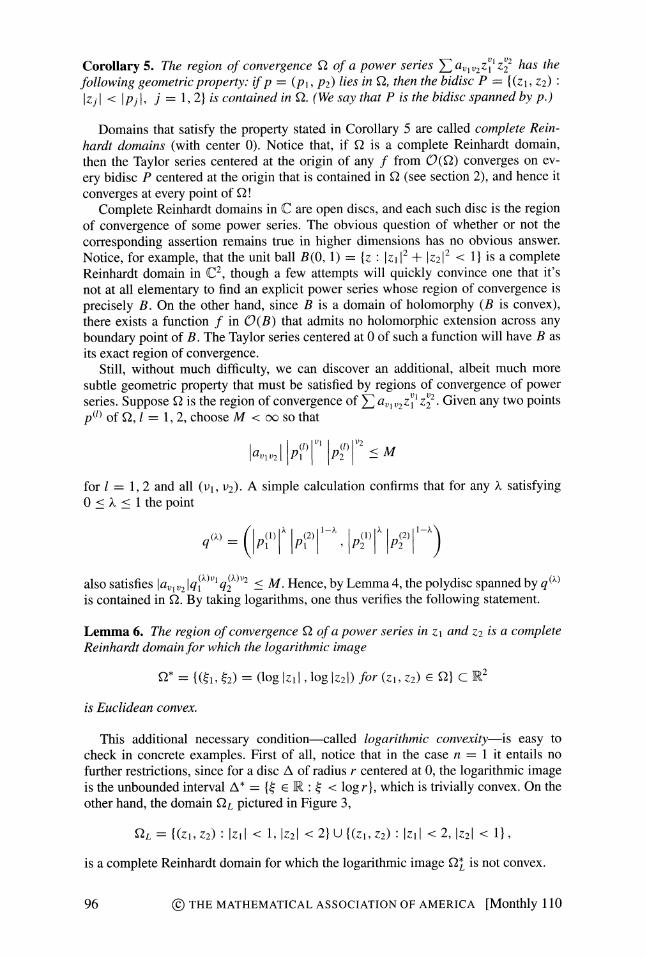
Corollary 5. The region of convergence 2 of a power series E av, VI' 2 has the

following geometric property: if p = (pi, P2) lies in Q2, then the bidisc P = {(zI, Z2)

zj I < Ipj , j = 1, 2} is contained in Q2. (We say that P is the bidisc spanned by p.)

Domains that satisfy the property stated in Corollary 5 are called complete Rein- hardt domains (with center 0). Notice that, if Q2 is a complete Reinhardt domain, then the Taylor series centered at the origin of any f from (9(2) converges on ev-

ery bidisc P centered at the origin that is contained in Q (see section 2), and hence it

converges at every point of Q2!

Complete Reinhardt domains in C are open discs, and each such disc is the region of convergence of some power series. The obvious question of whether or not the

corresponding assertion remains true in higher dimensions has no obvious answer. Notice, for example, that the unit ball B(0, 1) = {z : Iz 12 + 1Z21 < 1} is a complete Reinhardt domain in C2, though a few attempts will quickly convince one that it's not at all elementary to find an explicit power series whose region of convergence is

precisely B. On the other hand, since B is a domain of holomorphy (B is convex), there exists a function f in O(B) that admits no holomorphic extension across any boundary point of B. The Taylor series centered at 0 of such a function will have B as its exact region of convergence.

Still, without much difficulty, we can discover an additional, albeit much more subtle geometric property that must be satisfied by regions of convergence of power series. Suppose Q2 is the region of convergence of E av 2zI z2 ? Given any two points p(l) of 2, 1 = 1, 2, choose M < oo so that

l v 1 2 () (2 <M

for 1 = 1, 2 and all (vl, v2). A simple calculation confirms that for any X satisfying 0 < X < 1 the point

(h) = (IP (1) p(2) (1- ) 1 (2)1-X

q p i p1 P2 p i

also satisfies lav2 Iq(x)vl q()V2 < M. Hence, by Lemma 4, the polydisc spanned by q(X) is contained in Q2. By taking logarithms, one thus verifies the following statement.

Lemma 6. The region of convergence Q2 of a power series in zl and z2 is a complete Reinhardt domain for which the logarithmic image

Q* = {(1, ~2) = (log Izl , log 1z2 ) for (zl, Z2) E Q} C R2

is Euclidean convex.

This additional necessary condition-called logarithmic convexity-is easy to check in concrete examples. First of all, notice that in the case n = 1 it entails no further restrictions, since for a disc A of radius r centered at 0, the logarithmic image is the unbounded interval A* = {- X R : < log r}, which is trivially convex. On the other hand, the domain QL pictured in Figure 3,

2L = {(Zl, Z2): IZl < 1, IZ21 < 2} u {(Zi, Z2) Izll < 2, z21 < 1},

is a complete Reinhardt domain for which the logarithmic image Q2 is not convex.

() THE MATHEMATICAL ASSOCIATION OF AMERICA [Monthly 110 96

i l21z

--- log 2 /

1 2 Izll

L

L

Figure 3. A complete Reinhardt domain that is not logarithmically convex.

It follows that 2L is not the exact region of convergence of a power series, and consequently QL is not a domain of holomorphy. In fact, given f in O(2L), its Taylor series about the origin converges on QL, and therefore also on a region QL whose logarithmic image contains the convex hull of Q2. Thus f extends holomorphically to L.

The relationship of convergence properties with extension phenomena that we have seen in the foregoing examples is not accidental. Armed with more detailed knowl- edge, one can show that a logarithmically convex complete Reinhardt domain is indeed a domain of holomorphy-hence, by the same argument used earlier for the ball, the region of convergence of some power series. To summarize:

Theorem 7. The following statements are equivalent for a complete Reinhardt domain Q:

(i) Q2 is the exact region of convergence of a power series;

(ii) Q2 is logarithmically convex;

(iii) Q2 is a domain of holomorphy.

5. SINGULARITIES. The classification of isolated singularities is an important topic in complex analysis in the plane. Turning to higher dimensions, the corresponding theory all but vanishes: all isolated singularities are removable! This follows immediately from the Hartogs extension theorem. In fact, genuine singularities necessarily extend to the boundary of the open set under consideration. We shall briefly discuss two classes of nonisolated singularities that exhibit behavior analogous to familiar one variable scenarios.

Removable singularities. The first result generalizes the Riemann removable singularity theorem.

Theorem 8. Suppose that D is a domain in C" and that E is a subset of D with the following property: each point p of E has an open neighborhood Up such that E n Up is the zero set of a nontrivialfunction from O(Up). If f in O(D \ E) is bounded, then f extends holomorphically across E (i.e., f extends to a function in O(D)).


The proof is a rather simple application of the local description of zero sets that we discussed in section 2, and of the corresponding one-variable theorem. This result has the following neat topological consequence, which is rarely mentioned in one variable, because it is so obvious there: if E :A D is the zero set of a holomorphic function, then D \ E is connected! In fact, assume that D \ E = U1 U U2, where U1 and U2 are open and disjoint. Suppose U1 := 0. By the theorem, the holomorphic function on D \ E defined by f - 0 on U1 and f - 1 on U2 extends to a holomorphic function on D. By the identity theorem, f - 0 on D, whence U2 = 0!

Much more intriguing are the following two purely higher dimensional phenomena.

Theorem 9. Suppose that D is a domain in C" and that E is an analytic subset of D

of (complex) dimension at most n - 2. Then every f in 0(D \ E) extends holomor-

phically to D.

In other words, "analytic singularities" of dimension at most n - 2 are removable! Of course, we have not defined analytic sets and their dimension precisely. In simple situations the idea is clear, however. For example, E could be contained in a complex linear subspace of dimension no larger than n - 2, or in a finite union of such sub-

spaces. More generally, linear subspaces could be replaced by complex submanifolds of dimension n - 2 or smaller, a notion that will make sense to the reader familiar with real submanifolds. The proof is based on variations of techniques used in the proof of the local Hartogs extension phenomenon (Lemma 3).

Theorem 10. Suppose that D is a domain in C". If n > 2, then every f from O(D \ R") extends holomorphically to D.

The space RWn does not contain any nontrivial complex subspaces: it is the prototype of so-called totally real sets. Therefore this result is of a very different nature from the previous one. Its proof involves a clever application of logarithmic convexity (or, rather, the absence thereof) and power series. The crux is purely local. Assume that n = 2 and that we want to establish the extendability of f through some point of R2 in D-for simplicity, say the point is (0, 0). After appropriate rescaling of D we can assume that the translation L - (i, i) of the region 2L shown in Figure 3 is contained in (D\ IR2).5 Therefore the function h defined by h(zi, Z2) = f (Z - i, Z2 - i) is defined and holomorphic on QL. In section 4 we saw that the power series of h at the origin converges on a region QL that contains the point (i, i), i.e., that h has a

holomorphic extension to (i, i). This implies that f has a holomorphic extension to (0, 0).

Meromorphic functions and poles. Meromorphic functions are algebraic cousins of

holomorphic functions: they are objects that are locally described by quotients of holo-

morphic functions (with denominator not vanishing identically). When studying local

properties, it is thus enough to consider meromorphic functions of the form m = f/g, where f and g belong to 0(D). Clearly m has singularities only at points p for which

g(p) = 0. If f(p) :k 0 at such a point, the situation is analogous to the one variable case: one has limzp m(z) = oo (of course, in this limit we only consider z with

g(z) - 0), and the reciprocal 1/m = g/f is holomorphic at p with value 0. In this situation we say that the meromorphic function has a pole at p, and it makes sense to

assign to the function m the value oo at p. Just as in one variable, near a pole a mero-

morphic function may be recast as a continuous function into the Riemann sphere.

5The nonbelieving reader should check it out carefully. It will test his or her basic understanding of C2.

(? THE MATHEMATICAL ASSOCIATION OF AMERICA [Monthly 110 98

If, on the other hand, f(p) = g(p) = 0, the situation is more complicated. Again, the case n = 1 stands out for its simplicity: in this case one can cancel common factors z - p until either the denominator or the numerator of m is not zero at p. The singularity of f/g is thereby seen to be either a removable singularity or a pole. If n > 2, however, it is rare that cancellations occur. This fails already in the simplest examples, such as m(z) = Zl/Z2. Clearly every point (c, 0) with c := 0 is a pole of m, whereas one easily sees that the limit set of m(z) as z -> 0 is the full Riemann sphere. From the perspective of the one-variable theory one would have to say that 0 is an essential singularity of m, which surely overstates matters. Instead, one says in the context of several complex variables that 0 is a point of indeterminacy of the meromorphic function m. Any detailed further analysis of the singularities of meromorphic functions requires deeper algebraic techniques than we discuss here.

6. PSEUDOCONVEXITY. Hartogs's ground breaking discovery of open sets that are not domains of holomorphy immediately raises the issue of characterizing domains of holomorphy by more tractable equivalent properties. For example, we have already seen that within the class of complete Reinhardt domains, domains of holomorphy are characterized by a geometric condition, namely, logarithmic convexity. In essence, such a domain is a domain of holomorphy if and only if a particular snapshot of it is Euclidean convex. Surprisingly, the relationship to convexity persists in much more general situations, albeit in a more subtle guise-a phenomenon that is still not fully understood.

Levi pseudoconvexity. Already in 1910 E. E. Levi was investigating the properties of domains of holomorphy that had twice continuously differentiable boundaries, and he discovered a simple necessary condition for a domain to be a domain of holomorphy that bears striking formal similarities to the real differential characterisation of convexity (simplest case: the graph of a function y = f(x) is "convex" if and only if f" > 0). This condition is now known universally as the Levi condition, and the relevant property is known as Levi pseudoconvexity.

For the rest of this section we shall thus assume that the boundary bD of the region D is a C2-hypersurface, described locally in an open set U as the zero set bD n U = {z E U : r(z) = 0} of a C2-function r with nowhere vanishing gradient in U. Since the sign of r will matter, we shall specifically choose r so that r < 0 on D n U. Such a function r will be called a (local) defining function for D in U. Levi's first fundamental result states:

Theorem 11. Let r be a defining function for a domain D in an open set U. If D is a domain of holomorphy, then for each point p of bD n U it is the case that

n a2r

Lp(r; t) = a a-(P)tjtk > 0 j,k=l OZk

for all t in Cn that satisfy

E z (p)tj = O. j=1 azj

The condition on the vector t identifies a complex (n - 1)-dimensional subspace of C', which is called-in obvious analogy to the real case-the complex tangent


space Tji(bD) to bD at p. The space T (bD) is a subspace of the real tangent space of bD at p, itself a vector space of dimension 2n - 1 over I. The Hermitian form Lp(r, ) is called the Levi form (or complex Hessian) of r. It involves just routine arguments to verify that Levi pseudoconvexity (i.e., the property identified in the theorem) is

independent of the particular choice of defining function r, and also that-in contrast to Euclidean convexity-it is preserved under local holomorphic coordinate changes. It is elementary to verify directly that convex domains are Levi pseudoconvex, and it is obvious that every domain in C is Levi pseudoconvex.

The proof of the theorem is based on the following idea. Given p and t with

Lp(r; t) < 0, by making a suitable change of local holomorphic coordinates one can

explicitly construct a subregion H of D D U similar to the one appearing in Lemma 3 so that the associated "polydisc" contains the point p. As in Lemma 3, all holomorphic functions on D will then extend holomorphically to a neighborhood of p, meaning that D could not be a domain of holomorphy.

One says that D is strictly Levi pseudoconvex at the point p of bD if Lp(r; t) > 0 for all complex tangent vectors t : 0. Levi's second main result involves the following partial converse of the first theorem.

Theorem 12. Suppose that D is strictly Levi pseudoconvex at a boundary point p. Then there exists a neighborhood U of p such that D n U is a (weak) domain of holomorphy.

The main step of the proof is based on a careful analysis of the 2nd order Taylor expansion of a defining function r in order to construct a quadratic holomorphic polynomial Fp with Fp(p) = 0 such that {z E U nD : Fp(z) = 0} = {p}. Then 1/Fp, which belongs to O(D n U), is singular at p.

The Levi problem. Levi pseudoconvexity is the incarnation in the context of domains with C2-boundaries of a more general notion of pseudoconvexity for domains with ar-

bitrary boundaries. The details are quite a bit more complicated than in the case of Levi pseudoconvexity and will not be visited on this tour. Suffice it to say that every pseudoconvex open set can be exhausted from inside by strictly Levi pseudoconvex sets. Furthermore, pseudoconvexity is a local property of the boundary, that is, the statement that a domain is pseudoconvex if and only if it is pseudoconvex near every boundary point is, de facto, a tautology.

As you have probably guessed by now, pseudoconvexity is the crucial local property of the boundary that characterizes domains of holomorphy. In fact, Levi's pioneering work came very close to settling the problem for domains with differentiable boundaries, except for one major hurdle: even when D is strictly Levi pseudoconvex at

every boundary point p, Levi's second theorem produces a function singular at a given point p that is holomorphic only on D n U(p), where the neighborhood U is poten- tially quite small.6 But that is a far cry from finding a function f singular at p that is

holomorphic on the whole domain D! While in real analysis it is usually quite easy to

patch together local data in a smooth fashion-say by using Cx partitions of unity- because of the identity theorem these "soft analysis" tools are simply not available in

complex analysis. Levi, of course, recognized this difficulty, but he did not know how to overcome it. The question of whether or not a strictly pseudoconvex domain is indeed a domain of holomorphy resisted all efforts for the following thirty years, until the Japanese mathematician Kiyoshi Oka finally gave an affirmative answer in dimen-

6Just as in real calculus, the gap between the strict version and the general version is not that serious and is

easily overcome by appropriate refinements.

1() THE MATHEMATICAL ASSOCIATION OF AMERICA [Monthly 110 100

sion two in 1942. It took nearly another ten years until the case of arbitrary dimension was settled as well.

In contrast to the earlier (tautological) statement regarding pseudoconvexity, the

analogous statement that D is a domain of holomorphy if and only if it is locally a domain of holomorphy near every boundary point-obviously trivial in one direction-is

highly nontrivial in the other direction, where it incorporates, in particular, the solution of Levi's problem. The main consequence of the solution of Levi's problem is

captured by the statement that a subdomain D of C' is a domain of holomorphy (a global complex analytic property) if and only if it is pseudoconvex (a local "pseudo- geometric" property). It is fair to say that the solution of Levi's problem and its modem variations were a major Leitmotiv in complex analysis throughout most of the twentieth century. Even today, versions of Levi's problem in more abstract settings are still under investigation.

Pseudoconvexity versus convexity. As the Levi condition and its name suggest, pseudoconvexity is "somehow" a complex analogue of (Euclidean) convexity. The connec- tion is made concrete by the following neat and important geometric characterization: D is strictly Levi pseudoconvex at p if and only if there exist local holomorphic coordinates on a neighborhood U of p such that bD n U is a strictly Euclidean convex hypersurface (positive definite Hessian) with respect to the new coordinates. In other words, strict pseudoconvexity is exactly the local biholomorphic "image" of strict con-

vexity. The proof of this fact is elementary, but nontrivial. Does this characterization remain true in general? Generations of complex analysts grew up trusting that, in anal-

ogy with the strictly Levi pseudoconvex case, pseudoconvexity would be the local biholomorphic image of Euclidean convexity. Numerous surprising similarities and formal analogies between pseudoconvexity and Euclidean convexity nourished this faith, as mathematicians thoroughly investigated pseudoconvexity over the course of many decades. Even though no one knew a proof, it was widely believed-mostly in secret, not as an openly stated conjecture-that this geometric characterization should at least be correct in the case of differentiable boundaries. This belief was eventually shattered in 1972 when, quite to everybody's astonishment, J. J. Kohn and L. Nirenberg discovered a counterexample. Amazingly, the example is not at all pathological: it is defined by a rather simple polynomial of degree eight, and it enjoys other good properties.

The precise relationship between pseudoconvexity and convexity still remains a mystery. One of the major areas of investigations in complex analysis during the past thirty years involves the generalization of fundamental results concerning the boundary behavior of "analytic objects" from the known strictly Levi pseudoconvex case to more general pseudoconvex domains, say with smooth boundary.7 Notice that all domains in the plane with C2-boundaries are strictly Levi pseudoconvex, so one deals here with genuinely higher dimensional difficulties. Since the general terrain still looks quite intractable, the study of convex domains with smooth boundary, sort of an inter- mediate test case, has enjoyed a renaissance in recent years. Much of this work is

highly technical, and an exploration of its main features is best left for a separate tour.

7. BUILDING GLOBAL OBJECTS FROM LOCAL PIECES.

Origins and nature of the problem. The theorem of Mittag-Leffler and the Weier- strass product theorem are standard fare in any beginning complex analysis course.

7For emphasis, these are often referred to as weakly pseudoconvex domains.


Striking applications of the results include, for instance, the partial fraction decompo- sitions and the product representations of relevant trigonometric functions.

You may remember from your first complex analysis course that the main difficulty in the proofs of these classical theorems involves convergence problems. In fact, when one is given only finite local data-either principal parts for poles, or zeroes with multiplicities-the construction of the corresponding global object in dimension one is trivial. For example, to find a holomorphic function with zeroes at al, ..., al, just form the product H=I (z - aj). Extension of this simple idea to infinitely many zeroes requires nontrivial modifications to ensure that one ends up with a convergent infinite

product. In contrast, the analogous higher dimensional problem presents fundamental new

obstacles right from the start. They arise mainly because the zero sets of holomorphic functions are no longer isolated (not even compact) and because local information is no longer captured by simple global algebraic objects, as in dimension one, but is instead realized by local holomorphic functions. The nature of the problem is clearly visible when one considers, for example, just two local zero sets, as follows.

Clearly two functions f and g in O(U) describe the same zero set in U if and only if f/g belongs to 9* (U), where the latter notation signifies the set of units (nowhere zero functions) in the ring O(U). Now suppose that D = U1 U U2, and consider the (local) zero set data provided by functions fj in 0(Uj), j = 1, 2. To be able to "glue" their zero sets together, the data must be equivalent on the common region U12 = U1 n U2, i.e., one must require that f2/fl belongs to 0*(U12). Assuming that this necessary compatibility condition is satisfied, the zero set problem in this simple setting asks whether or not there is a global holomorphic function f on D whose zeroes in Uj are the same as those of fj, in other words, such that f/fj is in * (Uj) for j = 1, 2.

The answer is trivial in case fi = f2 on U12: then the local functions themselves, not just their zero sets, fit together correctly to yield a function f in 0(D) by defining f(z) = fj (z) for z in Uj. Of course, we will not usually be so lucky. Still, we have the freedom to multiply fj by a unit Uj from 0*(Uj) without changing the zero set. We can thus reformulate the question as follows: Can we find uj in 0*(Uj) for j = 1, 2 so that fl/ul = f2/u2 on U12? If this is the case, then defining f = fj/uj on Uj will produce the desired holomorphic function on D. The safest way to ensure that a function uj is invertible is to represent it as uj = exp gj. After rewriting the condition as u2/ul = f2/fi on U12, it readily translates into the condition

g2- gl = log(f2/fl) on U12

for unknown functions gj in 0(Uj). This latter additive condition is quite a bit simpler than the former multiplicative

problem. Another justification for focusing on this additive problem is provided by attempts to generalize the Mittag-Leffler theorem. Here the local data consist of meromorphic functions my on Uj for j = 1, 2, each of which describes the given "principal part" on Uj. Again, the data must match up on U12, a matter that in the present context is made precise by requiring that m2 - m = g12 be in O(U12). The problem then is to find a global meromorphic function m on D whose principal parts on

Uj are exactly the ones given by my, i.e., such that m - my is a member of O(Uj) for j = 1, 2. Since the prescribed principal parts are not altered if mj is replaced by mj - gj, where gj is an arbitrary function from 0(Uj), the question can be reformulated as follows: find gj in O(Uj) for j = 1, 2 so that ml - gl = m2 - g2 on U12, i.e., such that g2 - gl = g12(= m2 - ml) on U12. If there are such functions, defining m = mj - gj on Uj produces the desired global meromorphic function on D.

? THE MATHEMATICAL ASSOCIATION OF AMERICA [Monthly 110 102

Let us summarize the insight gained by our discussion. In order to extend classical

global results from the plane to higher dimensions one has to come to grips with a fundamental problem, namely, how to build up global analytic objects from finitely many local analytic pieces. Our discussion also suggests that this fundamental problem of patching together local data may be handled-at least in the simplest cases-by an

appropriate decomposition problem.

The basic decomposition problem. Straightforward generalization of the preceeding discussion leads to the following formulation in case infinitely many pieces of data are prescribed.

The Additive Problem. Let D be an open set in Cn. Suppose that {Uj : j = 1, 2, ...} is an open covering of D and that functions gjk in O(Uj n Uk) are given with the property that

gij + gjk + gki = 0

holds on Ui n Uj n Uk whenever Ui n Uj n Uk : 0. Findfunctions gj in O(Uj) such that gj - gi = gij on Ui n Uj.

The additional hypothesis is necessary for the conclusion to hold whenever there are at least three sets Uj. Note that it implies gii = 0 (set i j = k), and thus that

gjk = -gkj (seti = j). As we had already seen in the case of just two data pieces, solution of the additive

problem implies the generalization of the Mittag-Leffler theorem:

Corollary 13. For given D and open covering {Uj : j = 1, 2, .. .} of D, suppose that meromorphicfunctions mj on Uj are such that mk - mj belongs to O(Uj n Uk) whenever Uj n Uk :7 0. If the additive problem can be solved on D, then there exists a meromorphic function m on D such that m - mj is in 0(Uj) for j = 1, 2, ...

The generalization of the Weierstrass theorem follows as well, with a little twist. Given the covering {Uj : j = 1, 2, ...} of D and local "zero sets" associated with functions fj in 0(Uj) for which fk/fj belongs to O*(Uj n Uk), one applies logarithms to obtain the related additive problem. More precisely, one may assume that each Uj is a ball, making Uj n Uk simply connected. Hence one can choose in Uj n Uk a holomorphic branch gjk of log fk/fj. Note that this is not necessarily equal to log fk - log fj, since, by the very nature of the problem we are trying to solve, the functions fj will usually have zeroes in Uj n Uk. As a result it does not follow auto- matically that the functions gjk satisfy the condition gij + gjk + gki = 0 necessary for the solution of the additive problem. All one can say is that exp(gij + gjk + gki) = 1, i.e., gij + gjk + gki = nijk27ri for some integers nijk. One must carefully choose the branches of the logarithms to ensure that nijk = 0, a purely topological difficulty. As- suming that this can be done, the solution of the additive problem yields the functions

gj in 0(Uj). Just as was the case for two data pieces, defining f = fj/ exp gj on Uj produces a global holomorphic function on D with the locally prescribed zero set.

Incidentally, the potential topological obstruction we encountered in the foregoing discussion is indeed an unavoidable and fundamental feature of the higher dimensional zero set problem.8 It is invisible in dimension one, where the Weierstrass theorem holds on arbitrary regions. Subtle elementary examples show that the zero set problem may, for instance, fail to have a solution on the product of two annuli.

8More precisely, the obstruction lies in the cohomology group H2(D, Z), but that's a matter we shall not pursue further. Note that H2 (D, ) = 0 for an open set D in C.


From Cousin to Oka, and the triumph of analytic sheaf cohomology. The additive

problem, along with the applications to classical global function theory, was intro- duced in 1895 by the French mathematician Pierre Cousin, who succeeded in solving it for products D = D1 x ... x Dn of planar domains by systematically iterating one variable techniques based on the Cauchy integral formula.9 In his honor, the decom-

position problem is often referred to as the Additive Cousin Problem. Attempts to extend Cousin's theorem to more general regions face major obstacles.

Unfortunately, as we had already mentioned at the end of section 3, in higher dimensions there is no analogue of the Riemann mapping theorem. For example, a ball in C2 is not biholomorphically equivalent to a bidisc, or, more generally, to any product of

planar domains. Yet without a product structure, the one variable at a time approach of Cousin grinds quickly to a halt, and fundamental new ideas are needed. Unexpectedly, extension phenomena and domains of holomorphy make an unavoidable reappearance. For example, the solvability of the additive problem on a region D in C2 implies that D must be a domain of holomorphy! Thus domains of holomorphy turn out to be the natural setting for the solution of the central decomposition problem that arises in global multidimensional function theory.

Just as trekkers in the Himalayas are able to enjoy the sight of Mt. Everest and

appreciate the amazing skills of those who first reached its summit, our tour should include at least a brief admiring look at the marvelous accomplishments of Kiyoshi Oka. Blessed with penetrating insight and unusual technical skills, Oka set out in 1936 to conquer the most challenging unconquered complex analysis peaks of those times. We have already mentioned that Oka was the first to solve the Levi problem. Now we want to examine briefly how he solved the Cousin problem on domains of holomorphy.

From a distance, we can recognize the outline of Oka's route. As a consequence of the general theory of domains of holomorphy, it was known that such a domain D can be exhausted by an increasing sequence of analytic polyhedra, that is, by domains D1 of the type

D = zED: f (z) < 1, k =l,.., n

with compact closure in D, where the functions f) are holomorphic on D. This result is a complex analytic version of the familiar geometric fact that an open convex domain can be exhausted by (linear) convex polyhedra. (Recall: domains of holo-

morphy are pseudoconvex, a complex analogue of convexity.) The holomorphic map Fl = (f(l),..., f(l) : D -- Cnl provides a proper embedding of D1 as a complex submanifold of the unit polydisc p(nl) in Cnl. Oka's idea was to restrict the given additive data {gjk E O(Uj n Uk)} on D to the analytic polyhedron D), transport it via F() onto a submanifold of P(n), and then "extend" it to all of P(nl), where at last the desired decomposition could be found, thanks to Cousin's work. Finally, Oka needed to deal with the limit process D( -- D. In a remarkable tour-de-force, he succeeded in overcoming all obstacles along this route.

Soon after Oka's first breakthrough achievements, Henri Cartan vastly expanded the range of Oka's ideas, breaking new ground of his own. The difficult and often cumbersome details of Oka's techniques were generalized and crafted by Cartan into a cohesive and powerful tool that ultimately empowered ordinary mathematicians to climb efficiently and safely to the highest peaks. One of the marvelous creations of that period was the notion of a coherent analytic sheaf-a vast generalization of

9To handle the topological difficulty underlying the zero set problem, one needs to assume that all but one of the planar domains Dj are simply connected.

? THE MATHEMATICAL ASSOCIATION OF AMERICA [Monthly 110 104

Weierstrass's classic concept of analytic configuration built up from local germs of

holomorphic functions-and the corresponding sheaf cohomology theory. It is one of the wonders of twentieth century mathematics that sheaf cohomology, a formidable

algebraic-topological machine of great unifying power discovered by Jean Leray in the

early 1940s, turned out to provide the framework for the solution of classical problems in complex analysis, and for lifting complex analysis to new heights. The Oka-Cartan

theory became firmly established as one of the pillars of modem complex analysis.'1

8. OTHER ROUTES TO THE PEAKS. As we approach the end of our tour, we have come to recognize the pervasive roles that domains of holomorphy and the fundamental decomposition problems play in understanding familiar classical global problems. Other central phenomena, too, can be recast as such decomposition problems. For example, this is directly apparent in the proof of Hartogs's theorem in section 3, although the decomposition there required an additional twist involving control at in-

finity. Similarly, the solution of Levi's problem is an immediate consequence of such a decomposition result. In fact, if p lies in bD and if Q is a (strictly pseudoconvex) neighborhood of D, the quadratic holomorphic polynomial Fp of Levi (see Theorem 12 in section 6) defines a meromorphic function 1/Fp on U1 = Q2 U, while the function 0 is meromorphic in a neighborhood U2 of Q \ U. Solution of the Mittag-Leffler problem on Q produces a meromorphic function m on Q that has exactly the same

poles as the data {(1/Fp, U1), (0, U2)}; in particular, m is holomorphic on D and has a singularity at p.

It is clearly of major interest for complex analysis to find ways of solving the fundamental decomposition problem other than attacking it with the Oka-Cartan machinery. Beginning in the 1960s new routes were discovered that are in many ways much sim-

pler and closer to the hearts of analysts. We conclude this tour by taking brief looks at them.

The Cousin theorem via the Cauchy-Riemann equations. A by-product of the de-

velopments discussed at the end of the previous section was the discovery that the additive Cousin problem could easily be reformulated in terms of global solvability of the a-equation, i.e., of the Cauchy-Riemann equations.

Recall that for a C1-function f one defines the differential form af by af =

Of/azj dzj, and f is holomorphic if and only if a f = 0. Conversely, given co =

j gj dzj (an object known as a (0, l)-form), one asks whether co = f for some function f, in analogy with real calculus, where one asks if and when a differential 1-form is the differential of a function. To find such f, ct must clearly satisfy the necessary differential condition 8gj/azk = agk/a~j for j, k = 1, ... n. Just as in real calculus, it turns out that this condition is also sufficient for the existence of local solutions. Thus the heart of the matter deals with global existence results.

To illustrate the a-technique we give a a-proof of Cousin's additive theorem in the simple case of a covering of D by two sets Uj, j = 1, 2. Given f in O(U1 n U2), it is a routine analysis exercise, based on the existence of smooth cut-off functions, to solve the decomposition problem with C?-functions, that is, to find functions vj in

C??(Uj) such that v2 - v = f on U1 n U2.ll Of course avj := 0 now, but on U1 n U2

l?For example, solution of the additive Cousin problem on D is translated into the vanishing of H1 (D, 0), the first cohomology group of D with coefficients in the sheaf of germs of holomorphic functions. The general theory studies the cohomology groups with coefficients in arbitrary coherent analytic sheaves.

1 Note that U1 \ U2 and U2 \ U1 are disjoint (relatively) closed subsets of D = U1 U U2. Thus there exists X E CO(D) such that 0 < X < 1, X - 1 in a neighborhood of U2 \ U1, and X - 0 in a neighborhood of U1 \ U2. Then vl = -xf and v2 = (1 - x)f will do.


one has av2 - avl = f = 0, since f is holomorphic there. One thus obtains a global (0, l)-form co of class C? on D given by w = avj on Uj. Suppose that there is a

global solution u in C?(D) of au = co. Set gj = vj - u. Since gj = avj - au =

vj - c( = 0, it follows that gj belongs to 0(Uj) for j = 1, 2, and

g2 - g1 = (v2 - u) - (vl - u) = V2 - = f.

Essentially the same method of proof yields the following theorem.

Theorem 14. Suppose that an open set D of Cn has the following property: for every (0, 1)-form co of class CO? on D that satisfies the necessary integrability condition on D, there is a solution u in COO(D) of au = co. Then the additive Cousin problem is solvable on D, and consequently, the higher dimensional version of the Mittag-Leffler theorem holds on D.

The converse of the theorem holds as well.12 Thus the global solvability of the

a-equation on domains of holomorphy is a simple corollary of the Oka-Cartan theory. During the 1960s researchers in partial differential equations turned matters around

and successfully attacked the a-equation directly on pseudoconvex domains. Their results could then be applied to develop substantial portions of global multidimensional

complex analysis, expanding on the ideas underlying the theorem we just stated. In fact, this approach became enormously popular, fueled by L. Hormander's masterful

exposition in what has become, to date, the most widely used text in multidimensional complex analysis. In the decades since, substantial progress in a-techniques has led to the solution of numerous deep problems in complex analysis, particularly problems concerned with the refined boundary behaviour of complex analytic objects. Applications to complex analysis continue to provide a rich source of problems for

contemporary researchers in partial differential equations.

Global results by integral kernels. Once it was recognized in the 1960s that solutions of the Cauchy-Riemann equations made possible an ascent to the high peaks of

complex analysis, it became desirable from the perspective of a complex analyst to look for a new route to these wonderful a-methods that did not rely on the technical tools from PDE. Again, the roots go back to familiar results in the complex plane. Here the a-equation is just a simple scalar equation au/az = g. It is a classical fact that a solution to this equation in a domain D is generated by integrating g against the Cauchy kernel over the domain. This is a consequence of the following Cauchy integral formula for differentiable functions, which should really be a standard item in the syllabus for any elementary complex analysis course.l3

Theorem 15. Suppose that D is a domain in C with a piecewise C'-boundary and that f belongs to C1 (D). Then for z in D it is true that

f(z) f= f d( -- l fl a/() dA. 27ri JbD z - Z

12The proof is very simple. Since Au = w always has local solutions, there exist an open covering {Uj of D and functions uj in C??(Uj) such that auj = o on Uj. Then gjk = Uk - uj is holomorphic on Uj n Uk. By the additive Cousin theorem, there are functions gj in O(Uj) that satisfy gk - g = gjk. Hence Uk - gk =

uj - gj, i.e., the modified local solutions fit together to define a global solution.

13Incidentally, the proof involves just a standard application of Green's theorem.


Since the boundary integral defines a holomorphic function on D, one immediately obtains af/lz = /laz(TD(af/a))), where TD denotes the second integral operator on the right-hand side. Additional routine arguments prove that l8/z TD(g) = g for any reasonable g. Clearly the concrete formula for the solution TD(g) can be used to prove regularity results as well as to derive all sorts of estimates.

Attempts to generalize this simple procedure to higher dimensions encounter their own substantial difficulties. While we had seen straightforward generalizations of the Cauchy integral formula to polydiscs, no corresponding formula is readily available on more general domains. True, the Bochner-Martinelli kernel, which was mentioned in section 3, can be used to obtain an analog of Theorem 15; but this kernel is no longer holomorphic in z in more than one variable, so the procedure outlined to derive a solution of the a-equation from Theorem 15 breaks down. In fact, a crucial property of the Cauchy kernel-it is a holomorphic function with an isolated singularity at z = a-falls apart in higher dimensions. However, the holomorphic nature is critical only for the boundary integral. Since for a domain of holomorphy D there are indeed holomorphic functions on D with singularities at any specified point ~ of bD, the structural problem disappears in this case.

The situation is simplest in (Euclidean) convex domains. Here the appropriate integral formulas can be found in explicit, concrete form. None of this requires new tools beyond those available through a solid foundation in multivariable calculus and the systematic use of differential forms. Going beyond this elementary case, strictly pseudoconvex domains are the next logical class to consider, for they are locally convex in suitable coordinates. Again, one runs into a version of Levi's problem: one has to extend complex analytic objects from a local setting to a global setting. Thanks to improved "technology," it turns out that integral representations themselves allow a simple solution to this problem as well. Consequently, fundamental global results can now be reached directly by means of integral representations.

9. EPILOGUE. I hope that this tour has helped you to gain some insight into the fascinating world of complex analysis in higher dimensions. Should you wish to explore some of the topics more in detail, the following suggestions may be useful.

Rather than following the classical route to global theory via sheaf cohomology, I believe that a novice in multidimensional complex analysis who does not have much experience with partial differential equations would benefit most from the di- rect approach via integral representations, as found in the texts by G. M. Henkin and J. Leiterer [8] (especially the first two chapters) and by this author [14]. You should look at both texts and decide for yourself which style suits you best.

If you are experienced with partial differential equations, or are interested in learn- ing some of the related techniques, the best choice is L. Hormander's classic [10]. The presentation is elegant and complete, although less experienced analysts may need to put in extra effort. Other texts (for example, [7] and [11]) also include this material, but no one has been able to improve H6rmander's exposition. The recent book by S. C. Chen and M. C. Shaw [1] provides a long overdue update of a-techniques. In particular, it covers the boundary regularity theory of the a-Neuman problem, as well as many other newer developments, including an extensive discussion of the tangential Cauchy-Riemann equations, a concept central to more recent investigations.

The book by H. Grauert and K. Fritzsche [3] is an excellent introduction to the elements of multidimensional complex analysis, including coherent analytic sheaves, although it leaves proofs of many major results, especially the global ones, to more specialized literature. A completely revised and expanded new edition-with a new


title-has just been published [2]. It includes global results on complex manifolds that are obtained by power series methods rather than sheaf theory.

R. Narasimhan's lecture notes [13] provide another accessible introduction to many of the basic concepts, with particular emphasis on the Cartan-Thullen theory of domains of holomorphy in the context of Riemann domains.

S. Krantz's book [11] reflects its author's enthusiasm for analysis. It covers-in

varying degrees of depth and completeness-many of the basic concepts and results, and it also touches upon several topics not found in other books.

Should you wish to study complex spaces and the cohomology theory of coherent analytic sheaves, R. Gunning's trilogy [7], a substantially revised version of the 1965 classic by Gunning and H. Rossi, is a good place to start. The most complete and authoritative presentation is found in the excellent monographs of H. Grauert and R. Remmert [4], [5]. Before beginning either of these monumental works, I would recommend reading "Preview: Cohomology of Coherent Analytic Sheaves" in the author's book [14, sec. VI.6].

REFERENCES

1. S.-C. Chen and M.-C. Shaw, Partial Differential Equations in Several Complex Variables, AMS/IP Studies in Advanced Mathematics, vol. 19, American Mathematical Society, Providence, 2001.

2. K. Fritzsche and H. Grauert, From Holomorphic Functions to Complex Manifolds, Springer-Verlag, New

York, 2002. 3. H. Grauert and K. Fritzsche, Several Complex Variables, Springer-Verlag, New York, 1976. 4. H. Grauert and R. Remmert, Theory of Stein Spaces (trans. A. Huckleberry), Springer-Verlag, New York,

1979. 5. H. Grauert and R. Remmert, Coherent Analytic Sheaves, Springer-Verlag, New York, 1984. 6. M. B. Green, J. H. Schwarz, and E. Witten, Superstring Theory, vol. 2, Cambridge University Press,

Cambridge, 1987. 7. R. C. Gunning, Introduction to Holomorphic Functions of Several Variables, 3 vols., Wadsworth &

Brooks/Cole, Belmont, CA, 1990. 8. G. M. Henkin and J. Leiterer, Theory of Functions on Complex Manifolds, Birkhiuser, Boston, 1984. 9. G. M. Henkin and R. G. Novikov, The Yang-Mills Fields, the Radon-Penrose Transform and the Cauchy-

Riemann Equations, Several Complex Variables V, Encyclopedia of Mathematical Sciences, vol. 54, Springer-Verlag, Berlin, 1993.

10. L. H6rmander, An Introduction to Complex Analysis in Several Variables, Van Nostrand, Princeton, NJ, 1966; 3rd ed., North-Holland, Amsterdam, 1990.

11. S. Krantz, Function Theory of Several Complex Variables, John Wiley & Sons, New York, 1982; 2nd ed., Wadsworth, Belmont, CA, 1992.

12. Y. Manin, Gauge Field Theory and Complex Geometry, Springer-Verlag, Berlin, 1988. 13. R. Narasimhan, Several Complex Variables, University of Chicago Press, Chicago, 1971. 14. R. M. Range, Holomorphic Functions and Integral Representations in Several Complex Variables,

Springer-Verlag, New York, 1986; 2nd. corrected printing, 1998.

R. MICHAEL RANGE earned his Diplom in Mathematik at the University of G6ttingen, where lectures of Hans Grauert got him hooked on multidimensional complex analysis. A Fulbright Exchange Fellowship brought him to the United States and UCLA, where he received a Ph.D. in 1971. He has held academic positions at Yale University and at the University of Washington, as well as research positions at institutes in Bonn, Stockholm, Barcelona, and Berkeley. As befits his research interests and his guiding you on a tour to the

highlands of complex analysis, Range loves mountains and is an avid downhill skier. A few years ago, inspired and guided by his son, he got into ice climbing and alpine mountaineering. In the pursuit of other means to lift himself above the ground, he recently earned his pilot's certificate.

Department of Mathematics and Statistics, State University of New York at Albany, Albany, NY 12222

range @ math. albany. edu


Complex Analysis: A Brief Tour into Higher Dimensions · mathematics major in calculus of functions...

Documents

Transcript of Complex Analysis: A Brief Tour into Higher Dimensions · mathematics major in calculus of functions...