COMPILATION OF EXAMPLES – 13. ANALYTICAL …szeki/files/13_Peldatar_sikfeladatok_lektoralt... ·...

Dr. András Szekrényes, BME www.tankonyvtar.hu

COMPILATION OF EXAMPLES – 13. ANALYTICAL AND FINITE ELEMENT SOLUTION OF A PLATE

WITH CENTRAL HOLE

Author: Dr. András Szekrényes

2 Analytical and finite element solution of a plate with central hole

www.tankonyvtar.hu Dr. András Szekrényes, BME

13. ANALYTICAL AND FINITE ELEMENT SOLUTION OF A PLATE WITH CENTRAL HOLE

Calculate the stress field in the in-plane loaded plate with central hole shown in Fig.13.1 a. analytically by the help of the basic equations of elasticity, b. by finite element method using the code ANSYS, moreover, compare the results obtained from the two different calculations! The material of the plate is linear elastic, homogeneous and isotropic.

Fig.13.1. Plate with central hole subjected to normal load in direction x and tangential load along the boundaries.

13.1 Analytical solution The governing equation of plane problems has already been derived in cylindrical coordi-nate system in section 11 (see Eq.(11.74)):

011112

2

22

2

2

2

22

2224 =

∂∂

+∂∂

+∂∂

∂∂

+∂∂

+∂∂

=∇∇=∇ χϑϑ

χχrrrrrrrr

,

(13.1) which is a partial differential equation involving dynamic boundary conditions (formulated for the stress field). Accordingly, a boundary value problem should be solved. The stresses are expressed by the following equations (refer to section 11):

2

2

2

11ϑχχσ

∂∂

+∂∂

=rrrr , 2

2

r∂∂

=χσϑ ,

∂∂

∂∂

−=ϑχτ ϑ rrr

1 . (13.2)

The problem can be solved by the method of Fourier, i.e. it is assumed that the solution function is separable with respect to the variables [1]:

∑∞

=

Φ=1

)()(),(i

ii rRr ϑϑχ . (13.3)

Taking it back into the governing equation given by Eq.(13.1) we obtain:

http://www.tankonyvtar.hu/�

Alfejezetcím 3


01)(1)1(1)(1)(1432 =Φ+Φ ′′+Φ

+Φ

IVII R

rdrdRr

drd

rR

rdrdr

drd

rdrdRr

drd

rdrdr

drd

r.

(13.4) The solution in terms of variable r is searched in the form of a power function: nrrR =)( . (13.5) Taking it back into Eq.(13.4) the following is obtained: 0])2[()2( 2222 =Φ+Φ+−+Φ− IVIInnnn . (13.6) a. Let us assume that: IVII Φ=Φ , (13.7) which is possible only if Φ is the sum of constant and linear terms: ϑϑ 21)( CC +=Φ , (13.8) where C1 and C2 are constants. As a consequence Eq.(13.6) reduces to: 0)2( 22 =Φ−nn , (13.9) which is satisfied if n = 0 or 2, however each root is a double root due to the second power. The differential equation to be solved based on Eq.(13.4) is:

0)(1)(1=

drdRr

drd

rdrdr

drd

r. (13.10)

We integrate the equation with respect to r:

1)(1 cdrdRr

drd

rdrdr =

. (13.11)

As a next step we divide the equation by r and integrate again with respect to r:

21 ln)(1 crcdrdRr

drd

r+=

. (13.12)

Now we multiply the equation by r and integrate it third time:

3

2

21 2ln crcrdrrc

drdRr ++= ∫ . (13.13)

The partial integration of the first term on the right hand side yields:

3

2

2

22

1 2)

2ln(

21 crcrrrc

drdRr ++−= . (13.14)

We divide the result by r and integrate it even fourth time: DrCrrBArrR +++= lnln)( 22 , (13.15) where A, B, C and D are constants. Summarizing the results of case a. the elements of the basic function system are: { }1,ln,ln, 22 rrrr and { }1,ln,ln, 22 rrrrϑ . (13.16) These function, however are not periodic functions. It may be assumed that the solution function is periodic, i.e. it contains trigonometric functions. b. Because of the even derivatives we assume that the solution is the combination of trigo-nometric functions:

=Φ)sin()cos(

)(ϑϑ

ϑii

, (13.17)

accordingly:



−=Φ)sin()cos(

)( 2

ϑϑ

ϑii

iII ,

=Φ)sin()cos(

)( 4

ϑϑ

ϑii

iIV . (13.18)

From Eq.(13.6) we obtain: 0])2[()2( 422222 =++−+− inninn . (13.19) Let us investigate the possible values of parameter i! Eq.(13.19) is a second order equation for i2 of which solutions are:

{ }])2[(])2[(21 22222 nnnni −−±+−= , (13.20)

viz.:

−= 2

22

)2(nn

i . (13.21)

If n = 1 then for both cases the result is i2 = 1, i.e. for n = 1 we have double roots. The solu-tion in terms of r is R(r) = r, and the elements of the basic function system become: { }ϑϑϑϑϑϑ sin,cos,sin,cos rrrr . (13.22) From Eq.(13.21) we express the value of n in terms of i:

+±±

=2i

in . (13.23)

Let us investigate that in which cases we have double roots! If i = 1 then n = 1, -1, 3, 1, accordingly there exists one double root, and so the elements of the basic function system utilizing R(r) = rn are:

= rrr

rri ln,,1,:1 3 , (13.24)

where the last term is the fourth independent element due to the double root. If i = 2 then n = 2, -2, 4, 0, accordingly there is not any double root and the elements of the basic function system are:

= 1,,1,:2 4

22 r

rri . (13.25)

It can be seen based on Eq.(13.23) that if i > 1 then there is no double root, i.e. the solution can be presented in reduced form if i > 1. Let us summarize the solution function [1]!

),,(sincos

)lnln(

sin)(

cos)(

sin)ln1(

cos)ln1(

lnln),(

65

24

2321

2

24

2321

2

24

2321

143

131211

143

131211

204

2030201

ϑχϑϑϑϑ

ϑ

ϑ

ϑ

ϑ

ϑ

ϑχ

rrcrc

rrcrcrcc

irbrbrbrb

irararara

rrbrbr

brb

rrarar

ara

rrararaar

p

i

ii

ii

ii

ii

i

ii

ii

ii

ii

++++

+++++

+++++

+++++

+++++

+++++

++++=

∑

∑∞

=

−+−

∞

=

−+− (13.26)


Alfejezetcím 5


where the 1st, 6th and 7th rows contain the non-periodic solutions, rows 2nd-5th contain the periodic solutions when i = 1 and i = 2..∞. In the 7th row we included the missing terms due to the double roots for n = 1, finally the last term is the function of particular solution. Eventually, Eq.(13.26) can be applied to any plane problem on condition that we use cy-lindrical coordinate system. Let us get back now to the original problem! The stress tensor in a point sufficiently far from the hole is:

=

000000

,,

ttf

zyx

σ . (13.27)

We transform the stresses into the r-ϑ cylindrical coordinate system. The unit basis vectors of the cylindrical coordinate system are: jier ϑϑ sincos += and jie ϑϑϑ cossin +−= . (13.28) The radial stress based on the stress transformation expression is:

[ ] cstfcsc

ttf

scee rzyx

Trr 2

0000000

0 2

,,

+=

==∞ σσ , (13.29)

where c = cosϑ and s = sinϑ. Utilizing that cos2ϑ = 1/2⋅(cos(2ϑ)+1) and sin2ϑ = 2⋅cosϑ⋅sinϑ we obtain:

ϑϑσ 2sin)12(cos21 tfr ++=∞ . (13.30)

The tangential stress and the shear stress are calculated in a similar fashion:

ϑϑσσ ϑϑϑ 2sin)2cos1(21

,,

tfeezyx

T −−==∞ , (13.31)

ϑϑστ ϑϑ 2cos2sin21

,,

tfeezyx

Trr +−==∞ .

Comparing Eqs.(13.30)-(13.31) to the solution of Airy’s stress function in Eq.(13.26) the following terms remain:

,2sin)(

2cos)(

lnln),(

244

232

222

21

244

232

222

21

204

2030201

ϑ

ϑ

ϑχ

brbrbrbararara

rrararaar

++++

+++++

++++=

−

− (13.32)

which contains all in all twelve constants. Let us investigate the terms in the 1st row! The stress components become independent of ϑ, from Eq.(13.2) we obtain:

)1ln2(2110403202 +++=

∂∂

= raar

arrrχσ , (13.33)

)3ln2(2104032022

2

+++−=∂∂

= raar

arrχσ .

0=ϑτ r . The strain components are calculated using Hooke’s law for plane stress state based on Eq.(11.68):

)31(ln)1(2)1(2)1(1)( 040403202 νννννσσε ϑ −+−+−++=−= araar

aE rr ,

(13.34)



)3(ln)1(2)1(2)1(1)( 040403202 νννννσσε ϑϑ −+−+−++−=−= araar

aE r .

Moreover, the shear strain is zero. The relationship between the displacement field and the strain components is given by Eq.(11.66):

ru

r ∂∂

=ε , ru

=ϑε . (13.35)

We express the radial displacement, u from both equations:

rarrarar

aEudrruEdrE r )1(ln)1(2)1(2)1(1

04040302 ννννε +−−+−++−==∂∂

= ∫∫ ,

(13.36)

rarrarar

aEurE )3(ln)1(2)1(2)1(104040302 ννννεϑ −+−+−++−== ,

Comparing the results it is elaborated that the term after a04 leads to an incompatible dis-placement field. This contradiction can be resolved only if: 004 =a . (13.37) In the case of the other terms there are no compatibility problems. Next, we calculate the stresses considering all of the terms in Eq.(13.32):

,2sin)462(2cos)462(

2111

224

42221

224

422

221

032022

2

2

ϑϑϑχχσ

−−−− ++−++−

++=∂∂

+∂∂

=

rbrbbrarara

ar

arrrr

(13.38)

ϑϑχσϑ 2sin)62(2cos)62(21 42221

422

221032022

2−− +++++−=

∂∂

= rbbraraar

ar

,

ϑϑϑχτ ϑ 2cos)32(2sin)3(21 2

244

22212

244

2221−−−− −−−−−=

∂∂

∂∂

−= rbrbbraraarrr ,

where we can notice that the terms a23 and b23 vanish, which can be explained mathemati-cally by the fact that for r = ∞ finite stresses are required. There are still eight unknown constants in the stress formulae. These eight constants can be obtained based on the boundary conditions of the problem. We incorporate Eqs.(13.30) and (13.31), which give the stress state at any point, which is located at an infinitely far r distance from the hole:

ϑϑϑϑϑσσ 2sin22cos222sin2cos21

21),( 212103 baatffrr −−=++⇒∞=∞ ,

(13.39)

ϑϑϑϑϑσσ ϑϑ 2sin22cos222sin2cos21

21),( 212103 baatff ++=−−⇒∞=∞ ,

and this yields:

fa41

03 = , fa41

21 −= , tb21

21 −= . (13.40)

Further five constants can be calculated based on the dynamic boundary conditions. If r = R then the hole is free to load independently of the angle coordinate ϑ, consequently:


Alfejezetcím 7


=++−

=++−

=+

⇒=

01416

014162

0211

0),(

224422

224422

202

Rb

Rbt

Ra

Raf

fr

a

Rr ϑσ , (13.41)

=−−−

=−−−⇒=

01132

011320),(

224422

224422

Rb

Rbt

Ra

Raf

Rr ϑτ ϑ .

The solutions of the system of equations are:

2

2

02Rfa −= ,

4

4

22Rfa −= ,

2

2

24Rfa = ,

2

4

22Rtb −= , 2

24 tRb = .

(13.42) Taking the constants back into the stress formulae we obtain:

ϑϑϑσ 2sin)341(2cos)341(2

)1(2

),( 4

4

2

2

4

4

2

2

2

2

rR

rRt

rR

rRf

rRfrr +−++−+−= ,

(13.43)

ϑϑϑσϑ 2sin)31(2cos)31(2

)1(2

),( 4

4

4

4

2

2

rRt

rRf

rRfr +−+−+= ,

ϑϑϑτ ϑ 2cos)321(2sin)321(2

),( 4

4

2

2

4

4

2

2

rR

rRt

rR

rRfrr −++−+−= .

To plot the functions of stress field let us perform the function analysis of the solution! I. ϑ = 90°, this leads to:

fffR 3)31(2

)11(2

)( =+++=ϑσ , (13.44)

ffffR 22,132/39)16/31(2

)4/11(2

)2( ==+++=ϑσ ,

ffffR 037,1516/531)256/31(2

)16/11(2

)4( ==+++=ϑσ ,

0)( =Rrσ - dynamic boundary condition. II. ϑ = 0°, cos(2ϑ) = 1, sin(2ϑ) = 0, i.e:

)341(2

)1(2

)( 4

4

2

2

2

2

rR

rRf

rRfrr +−+−=σ , (13.45)

moreover, if r = R then σr(r) = 0, which is also a dynamic boundary condition. Let us search the extreme value of σr(r):

0))4(324(22

2)(5

4

3

2

3

2

0

=−+⋅+== r

RrRf

rRf

drrd r

ϑ

σ , (13.46)

from which we obtain Rr 2,1= . Taking it back and calculating the extreme value we have:

fffRr 0417,0)2,113

2,1141(

2)

2,111(

2)2,1( 2 −=+−+−=σ .



(13.47) Let us calculate the root of the function:

03411 4

4

2

2

2

2

=+−+−rR

rR

rR , (13.48)

which yields Rr 5,1= . Finally, if ∞⇒r then fr =σ . III. Along the circumference of the hole there is a uniaxial stress state, which is justified

by the followings: 0),( =ϑσ Rr and 0),( =ϑτ ϑ Rr due to the dynamic boundary conditions, further-

more:

ϑϑϑσϑ 2cos22cos)31(22

),( ffffR −=++= , (13.49)

and based on 02cos21 =− ϑ the root of this function is calculated from: 302/12cos =⇒= ϑϑ .

IV. If f = 0 and there is only tangential load t, then at r = R we have 0),(),( == ϑτϑσ ϑ RR rr and ϑϑσϑ 2sin4),( tR −= .

The results are presented in Figs.13.2 and 13.3. We note that the problem of plate with central hole can be solved also by complex variable functions, see e.g. [2,3].

Fig.13.2.Tangential stresses if ϑ = 90° and radial stresses if ϑ = 0° in a plate with central hole.


Alfejezetcím 9


Fig.13.3.Tangential stresses in a plate with circular hole subjected to uniaxial tension in direction x (a) and tangential load along the boundaries (b).

13.2 Finite element solution Solve the problem of the plate with central hole shown in Fig.13.4 by the finite element method! Prepare the finite element model of the plate depicted in the figure; calculate the nodal displacements and stresses! Plot the distribution of normal and shear stresses along the symmetry lines!

Fig.13.4. Finite dimension plate with central hole subjected to uniaxial tension and tangential load.

Given: A = 80 mm, R = 8 mm, f = 1 MPa, t = 1 MPa, E = 200 GPa, ν = 0,3, v = 1 mm



The finite element solution is presented by using the code ANSYS 12. The actual com-mands are available in the left hand side and upper vertical menus [4]. The distances are defined in [mm], the force is given in [N].

File menu / Change Title / Title: “Modeling of a plate with hole under plane stress state” Printing the problem title on the screen

- refresh the screen by the mouse roller

PREFERENCES – STRUCTURAL Analysis type definition

PREPROCESSOR / ELEMENT TYPES / ADD/EDIT/DELETE /ADD / SOLID / QUAD Element type definition – 4 node isoparametric plane element (PLANE42)

4NODE 42 / OK / PREPROCESSOR / OPTIONS / ELEMENT BEHAVIOR K3 – PLANE STRS W/THK /

OK / CLOSE PREPROCESSOR / REAL CONSTANTS / ADD/EDIT/DELETE / ADD / OK / THK=1 /

OK / CLOSE – definition of the thickness

PREPROCESSOR / MATERIAL PROPS / MATERIAL MODELS / STRUCTURAL / Material properties definition

LINEAR / ELASTIC / ISOTROPIC / EX = 200e3, PRXY = 0.3 / OK Exit: Material menu / Exit

PREPROCESSOR / MODELING / CREATE / AREAS / RECTANGLES / BY 2 COR-NERS / WPX = 0, WPY = 0, WIDTH = 20, HEIGHT = 20

Geometry preparation

- definition of the coordinates in the opening window Click the 9th icon on the right entitled „Fit View”, it fits the screen to the actual object size. PREPROCESSOR / MODELING / CREATE / AREAS / RECTANGLES / BY 2 COR-NERS / WPX = 0, WPY = 0, WIDTH = 80, HEIGHT = 80 / APPLY Creation of a further square PREPROCESSOR / MODELING / CREATE / AREAS / RECTANGLES / BY 2 COR-NERS / WPX = 20, WPY = 20, WIDTH = 60, HEIGHT = 60 / OK Elimination of the overlapping areas PREPROCESSOR / MODELING / OPERATE / BOOLEANS / OVERLAP / AREAS / PICK ALL Creation of the hole PREPROCESSOR / MODELING / CREATE / AREAS / CIRCLE / SOLID CIRCLE /

WPX = 0, WPY = 0, RADIUS = 8 / OK Subtraction of the hole from the smaller square


Alfejezetcím 11


PREPROCESSOR / MODELING / OPERATE / BOOLEANS / SUBTRACT / AREAS - selection of the smaller square by the mouse / OK - selection of the circle by the mouse / OK

Bisection of the quarter arc of the hole PREPROCESSOR / MODELING / OPERATE / BOOLEANS / DIVIDE / LINE W/OPTIONS / OK /

- selection of the arc / OK Connection of the quarter arc midpoint with the corner of the smaller square by a straight line PREPROCESSOR / MODELING / CREATE / LINES / LINES / STRAIGHT LINE –

- selection of the points by the mouse / OK Division of the smaller area by the line with inclination of 45° PREPROCESSOR / MODELING / OPERATE / BOOLEANS / DIVIDE / AREA BY LINE - selection of the smallest area / OK - selection of the line with inclination angle of 45°/ OK Fig.13.5 shows the process of creating the areas.

Fig.13.5. Preparation of the geometrical model of a plate with central hole.

Reflection of the model with respect to axis x PREPROCESSOR / MODELING / REFLECT / AREAS / PICK ALL / X-Z PLANE Y / OK Glue the areas to each other PREPROCESSOR / MODELING / OPERATE / BOOLEANS / GLUE / AREAS / PICK ALL

Element number definition along the lines based on Fig.13.6 Meshing

PREPROCESSOR / MESHING / SIZE CNTRLS / MANUALSIZE / LINES / PICKED LINES / PICK / NO. OF ELEMENT DIVISIONS = typing in the proper number, repetition of the command

PREPROCESSOR / MESHING / MESH / AREAS / MAPPED / 3 OR 4 SIDED / PICK ALL



Plot menu / Multi-Plots – display the elements and nodes

Fig.13.6. Details of the finite element model of the plate with central hole.

Reflection of the model with respect to axis y PREPROCESSOR / MODELING / REFLECT / AREAS / PICK ALL / Y-Z PLANE X / OK Glue the areas to each other PREPROCESSOR / MODELING / OPERATE / BOOLEANS / GLUE / AREAS / PICK ALL Elimination of the overlapping nodes along the vertical symmetry line PREPROCESSOR / NUMBERING CTRLS / MERGE ITEMS / TOLER Range of coinci-dence = 0.05 / OK

Load case 1: f = 1 MPa distributed load in direction x Loading definition, load cases

Kinematic constraints PREPROCESSOR / LOADS / DEFINE LOADS / APPLY / STUCTURAL /

DISPLACEMENT / ON NODES - selection of the lowest point on the vertical symmetry line / OK / UX, UY / APPLY - selection of the highest point on the vertical symmetry line / OK / UX / OK

Definition of f = 1 MPa PREPROCESSOR / LOADS / DEFINE LOADS / APPLY / STUCTURAL / PRESSURE / ON LINES /


Alfejezetcím 13


- selection of the lines with coordinate x = 40 and -40 mm by the mouse, intensity, VALUE Load PRES Value = -1

Read the load case as load step 1 (LS1) PREPROCESSOR / LOADS / LOAD STEP OPTS / WRITE LS FILES / LSNUM = 1 Deletion of the load and kinematic constraints PREPROCESSOR / LOADS / DEFINE LOADS / DELETE / STUCTURAL / PRESSURE / ON LINES / PICK ALL PREPROCESSOR / LOADS / DEFINE LOADS / DELETE / STUCTURAL / DIS-PLACEMENT / ON NODES / PICK ALL / ALL DOF / OK Load case 2: t = 1 MPa tangentially distributed load PREPROCESSOR / LOADS / DEFINE LOADS / APPLY / STUCTURAL / PRESSURE /

ON ELEMENTS - activation of the „box”, selection of elements on the right side on the upper longer horizontal boundary by the box / OK LKEY = 4, VALUE LOAD PRES VALUE = 1 / APPLY - activation of the „box”, selection of elements on the right side on the upper smaller horizontal boundary by the box / OK LKEY = 1, VALUE LOAD PRES VALUE = 1 / APPLY - activation of the „box”, selection of elements on the right side on the lower smaller horizontal boundary by the box / OK LKEY = 3, VALUE LOAD PRES VALUE = 1 / APPLY - activation of the „box”, selection of elements on the right side on the lower longer horizontal boundary by the box / OK LKEY = 3, VALUE LOAD PRES VALUE = 1 / APPLY

Along the other boundaries the load should be defined according to Fig.13.7a, where we gave the values of LKEY for all of the boundary lines. The load is equal to unity on each boundary line.



Fig.13.7. Definition of the LKEY parameter for the boundary lines of finite element model of the plate with central hole (a), definition of the boundary conditions by rotating the model (b).

Kinematic constraint, we create a local coordinate system, see Fig.13.7b. PREPROCESSOR / MODELING / CREATE / KEYPOINT / IN ACTIVE CS / x = 0, y = 0, z = 0 / OK Workplane menu / Local Coordinate Systems / Create Local CS / By 3 Keypoints +

- selection of the point with coordinates x = 40 mm, y = 40 mm - selection of the point with coordinates x = 0, y = 0 - selection of the point with coordinates x = -40 mm, y = 40 mm / OK

Display the model in coordinate system 11 Workplane menu / Change Display CS to / Specified Coord Sys / KCN = 11 / OK (refresh the screen by the mouse roller) PREPROCESSOR / LOADS / DEFINE LOADS / APPLY / STUCTURAL / DIS-PLACEMENT / ON NODES

- select the node with coordinates x = 0, y = 0 / OK / UX, UY / AP-PLY - select the node with coordinate 802 ⋅=x mm, y = 0 / OK / UY / OK

Read the load case as load step 2 (LS2) PREPROCESSOR / LOADS / LOAD STEP OPTS / WRITE LS FILES / LSNUM = 2

SOLUTION / SOLVE / FROM LS FILES / 1 – 2 Solution

„SOLUTION IS DONE!” Set the active and display coordinate system Workplane menu / Change Active CS to / Global Cartesian Workplane menu / Change Display CS to / Global Cartesian (refresh the screen by the mouse roller)

GENERAL POSTPROC / LOAD CASE / CREATE LOAD CASE / from Results file/ OK Creation of load cases, read and multiplication

LCNO = 1, LSTEP = 1, SBSTEP = Last / APPLY / OK LCNO = 2, LSTEP = 2, SBSTEP = Last / OK Read load cases GENERAL POSTPROC / LOAD CASE / READ LOAD CASE 1 – normal load (f) GENERAL POSTPROC / LOAD CASE / READ LOAD CASE 2 – tangential load (t)

GENERAL POSTPROC / PLOT RESULTS / DEFORMED SHAPE / select DEF + UNDEF EDGE / OK

Plotting and listing of the results


Alfejezetcím 15


PlotCtrls menu / Animate / Deformed Shape - animation Nodal displacements, stresses and strains with color scale GENERAL POSTPROC / PLOT RESULTS / CONTOUR PLOT / NODAL SOLU / NODAL SOLUTION: nodal displacements DOF SOLUTION: UX, UY, USUM displacements with color scale STRESS: normal and shear stresses, principal stresses,

equivalent stresses ELASTIC STRAIN: strains and shear strains, principal strains

equivalent strains Stresses, strains, element solutions with color scale GENERAL POSTPROC / PLOT RESULTS / CONTOUR PLOT / ELEMENT SOLU / ELEMENT SOLUTION: element solutions STRESS: normal and shear, principal stresses, equiva-

lent stresses ELASTIC STRAIN: strains and shear strains, principal strains,

equivalent strains Display the results in cylindrical coordinate system GENERAL POSTPROC / OPTIONS FOR OUTP / RSYS Results coord system / Global cylindrical The stress distributions are demonstrated in Fig.13.8 for the load case with uniaxial ten-sion in x. The model is symmetric, therefore we present only the one half of it.



Fig.13.8. Stresses in the finite element model of the plate with hole in [MPa], σx (a) and σy (b) in the x-y coordinate system and σϑ (c) in cylindrical coordinate system.

Displacements, stresses, strains along a predefined path GENERAL POSTPROC / PATH OPERATIONS / DEFINE PATH / BY NODES

- selection of the starting and ending nodes of the vertical symmetry axis / OK / - Name: ST90

GENERAL POSTPROC / PATH OPERATIONS / MAP ONTO PATH

- STRESS / X-DIRECTION, SX - selection of the normal stress in x

GENERAL POSTPROC / PATH OPERATIONS / PLOT PATH - display the path by white line

GENERAL POSTPROC / PATH OPERATIONS / PLOT PATH ITEM / ON GRAPH

- display the distribution Changing the setup of diagram PlotCtrls menu / Style / Graphs / Modify Axes (The other stress components can be plotted in a same way) Similarly to Figs.13.2 and 13.3 we show the stresses calculated by the finite element meth-od. The results are shown in Figs.13.9 and 13.10a.

Fig.13.9. Tangential stresses in the plate for ϑ = 90°and radial stresses for ϑ = 0° obtained by the finite element solution.

The results for load case 2 can be processed by repeating the commands above. The results can also be listed. As an example let us see how to list the stresses along the central hole if the plate is subjected to “t” tangential load only.


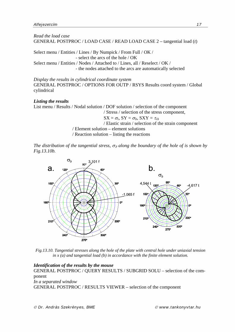
Alfejezetcím 17


Read the load case GENERAL POSTPROC / LOAD CASE / READ LOAD CASE 2 – tangential load (t) Select menu / Entities / Lines / By Numpick / From Full / OK /

- select the arcs of the hole / OK Select menu / Entities / Nodes / Attached to / Lines, all / Reselect / OK /

- the nodes attached to the arcs are automatically selected Display the results in cylindrical coordinate system GENERAL POSTPROC / OPTIONS FOR OUTP / RSYS Results coord system / Global cylindrical Listing the results List menu / Results / Nodal solution / DOF solution / selection of the component / Stress / selection of the stress component,

SX = σr, SY = σϑ, SXY = τrϑ / Elastic strain / selection of the strain component / Element solution – element solutions / Reaction solution – listing the reactions The distribution of the tangential stress, σϑ along the boundary of the hole of is shown by Fig.13.10b.

Fig.13.10. Tangential stresses along the hole of the plate with central hole under uniaxial tension in x (a) and tangential load (b) in accordance with the finite element solution.

Identification of the results by the mouse GENERAL POSTPROC / QUERY RESULTS / SUBGRID SOLU – selection of the com-ponent In a separated window GENERAL POSTPROC / RESULTS VIEWER – selection of the component



13.3 Comparison of the results by analytical and finite element solutions The stress distributions obtained from the two different solutions agree very well. Consid-ering the finite element results in Fig.13.2 and the analytical results in Fig.13.9, respective-ly, there are only small differences in the stress distributions. The radial stress changes its sign if Rr 5,1= in accordance with the analytical solution (see Fig.13.2). On the contrary, there is no change in the sign according to the finite element solution (see Fig.13.9), which can be explained by the fact that the resolution of the finite element mesh is not fine enough in the corresponding part. The stress distributions along the circumference of the hole are presented in Figs.13.3 and 13.9 obtained from analysis and finite element calcula-tion, respectively. The analytical and finite element solutions provide the same intersection points, where the stresses are equal to zero. Considering the maximum and minimum val-ues of the stresses there are some differences, but these are not significant discrepancies.

13.4 Bibliography [2] Gábor Vörös, Lectures and practices of the subject Applied mechanics, manuscript,

Budapest University of Technology and Economics, Faculty of Mechanical Engi-neering, Department of Applied Mechanics, 1978, I. semester, Budapest (in Hun-garian).

[2] L.P Kollár, G.S. Springer, Mechanics of composite structures, Cambridge Universi-ty Press 2003, Cambridge, New York, Melbourne, Madrid, Cape Town, Singapore Sao Pãolo.

[2] György Kozmann, Strength of materials of beams with varying cross section, Engi-neering Training Institute, lecture series from 1953-54: 2707, 1954, manuscript (in Hungarian).

[4] ANSYS 12 Documentation. http://www.ansys.com/services/ss-documentation.asp.


http://www.ansys.com/services/ss-documentation.asp�

COMPILATION OF EXAMPLES – 13. ANALYTICAL …szeki/files/13_Peldatar_sikfeladatok_lektoralt... ·...

Documents

Transcript of COMPILATION OF EXAMPLES – 13. ANALYTICAL …szeki/files/13_Peldatar_sikfeladatok_lektoralt... ·...