COMPETITIVE LEARNING NEURAL NETWORK ENSEMBLE...

COMPETITIVE LEARNING

NEURAL NETWORK ENSEMBLE

WEIGHTED BY PREDICTED PERFORMANCE

by

Qiang Ye

Bachelor of Engineering, Hefei University of Technology, 1997

Master of Science, University of Pittsburgh, 2003

Submitted to the Graduate Faculty of

School of Information Sciences in partial fulfillment

of the requirements for the degree of

Doctor of Philosophy

University of Pittsburgh

2010

ii

UNIVERSITY OF PITTSBURGH

SCHOOL OF INFORMATION SCIENCES

This dissertation was presented

by

Qiang Ye

It was defended on

March 5th

, 2010

and approved by

Stephen Hirtle, PhD, Professor, School of Information Sciences

Hassan Karimi, PhD, Associate Professor, School of Information Sciences

Satish Iyengar, PhD, Professor, Department of Statistics

Bambang Parmanto, PhD, Associate Professor, School of Health & Rehabilitation Sciences

Dissertation Director: Paul Munro, PhD, Associate Professor, School of Information Sciences

iii

Copyright © by Qiang Ye

2010

iv

COMPETITIVE LEARNING NEURAL NETWORK ENSEMBLE

WEIGHTED BY PREDICTED PERFORMANCE

Qiang Ye, PhD

University of Pittsburgh, 2010

Ensemble approaches have been shown to enhance classification by combining the outputs from

a set of voting classifiers. Diversity in error patterns among base classifiers promotes ensemble

performance. Multi-task learning is an important characteristic for Neural Network classifiers.

Introducing a secondary output unit that receives different training signals for base networks in

an ensemble can effectively promote diversity and improve ensemble performance. Here a

Competitive Learning Neural Network Ensemble is proposed where a secondary output unit

predicts the classification performance of the primary output unit in each base network. The

networks compete with each other on the basis of classification performance and partition the

stimulus space. The secondary units adaptively receive different training signals depending on

the competition. As the result, each base network develops “preference” over different regions of

the stimulus space as indicated by their secondary unit outputs. To form an ensemble decision,

all base networks’ primary unit outputs are combined and weighted according to the secondary

unit outputs. The effectiveness of the proposed approach is demonstrated with the experiments

on one real-world and four artificial classification problems.

Keywords: ensemble, diversity, neural networks, competitive learning, multi-task learning, bias

and variance, classification

v

TABLE OF CONTENTS

1. Introduction ........................................................................................................................... 1

1.1 Classification Background .............................................................................................. 1

1.2 Types of Classifiers ........................................................................................................ 2

1.2.1 Bayes Classifier ................................................................................................. .2

1.2.2 Tree Classifier .................................................................................................... .3

1.2.3 Backpropagation Neural Network Classifier ....................................................... .3

1.2.4 Choice of Classifiers .......................................................................................... .5

1.3 Neural Network Ensemble Methods ................................................................................ 5

1.4 Organization of the Paper ............................................................................................... 7

2. Bias and Variance Decomposition ......................................................................................... 8

2.1 Bias and Variance Decomposition for Single Classifiers ................................................. 8

2.2 Bias, Variance and Covariance Decomposition for Ensembles ........................................ 9

3. Previous Research on Ensemble Methods ............................................................................ 11

3.1 Varying Training Data .................................................................................................. 11

3.2 Varying Input Features ................................................................................................. 13

3.3 Varying Architecture .................................................................................................... 16

3.4 Varying Initial Conditions ............................................................................................ 17

4. The Multi-Task Learning Neural Network Ensemble ........................................................... 18

4.1 The Multi-Task Learning Ensemble Mechanism ........................................................... 18

4.2 Evaluation of the Multi-Task Learning Ensemble ......................................................... 20

5. The Proposed Approach – A Competitive Learning Neural Network Ensemble ................... 23

vi

6. Evaluation and Experiment Design ...................................................................................... 26

6.1 The Baseline ................................................................................................................. 26

6.2 The Datasets ................................................................................................................. 27

6.3 Evaluation of the Ensemble Classification Error ........................................................... 27

6.4 Evaluation of the Secondary Unit Performance ............................................................. 27

6.5 Evaluation of the Ensemble Diversity ........................................................................... 28

6.6 Evaluation of the Classification Error Decomposition ................................................... 28

7. Experiment Results and Discussion ..................................................................................... 30

7.1 The Experiment on the 2-D Annulus Classification Problem ......................................... 30

7.1.1 Illustration of the Annulus Datasets .................................................................. .31

7.1.2 Experiment Implementations ............................................................................ .33

7.1.3 Evaluation of the Misclassification Performance .............................................. .33

7.1.4 Visualization of the Network Preference Map .................................................. .35

7.1.5 Visualization of the Ensemble Outputs and the ROC Curves ............................ .36

7.1.6 Evaluation of the Secondary Unit Performance ................................................ .41

7.1.7 Evaluation of the Ensemble Diversity ................................................................ 42

7.1.8 Evaluation of the Classification Error Decomposition ...................................... .43

7.2 The Experiment on the Checkerboard Classification Problem ....................................... 44


7.2.2 Performance Evaluation ................................................................................... .46

7.3 The Experiment on the 10-D Parity Classification Problem .......................................... 50



7.3.3 The Distribution of “Winner Networks” ........................................................... .52

7.4 The Experiment on the Synthetic Diabetes Problem ...................................................... 57



7.5 The Experiment on the SPECT Heart Classification Problem ........................................ 63



vii

7.6 Experiments Summary .................................................................................................. 65

8. Conclusion and Future Directions ........................................................................................ 67

Bibliography ............................................................................................................................ 70

viii

LIST OF TABLES

Table 1.1 An ideal classifier ensemble ....................................................................................... 6

Table 7.1 The type I and type II errors by classification thresholds .......................................... 38

Table 7.2 The pair-wise distance matrix for the 10-D parity problem ....................................... 53

Table 7.3 The cumulative percentage by pair-wise distance for the 10-D parity problem ......... 53

Table 7.4 The correlation matrix of the original diabetes dataset ............................................. 58

Table 7.5 The correlation matrix of the synthetic diabetes dataset ............................................ 58

Table 7.6 Mean misclassification rate comparison for all five datasets ..................................... 65

ix

LIST OF FIGURES

Figure 1.1 A schematic of a feed-forward neural network with two hidden layers .................... 4

Figure 1.2 The architecture of a classifier ensemble ................................................................. 6

Figure 4.1 A base network with two output units ................................................................... 19

Figure 4.2 The MTL ensemble .............................................................................................. 20

Figure 4.3 The MTL ensemble vs. the standard ensemble ...................................................... 22

Figure 5.1 A competitive learning neural network ensemble .................................................. 24

Figure 7.1 Illustration of the annulus task with no noise ........................................................ 31

Figure 7.2 Illustration of the annulus task with small noise .................................................... 32

Figure 7.3 Illustration of the annulus task with large noise ..................................................... 32

Figure 7.4 Misclassification comparison – no noise ............................................................... 33

Figure 7.5 Misclassification comparison – small noise .......................................................... 34

Figure 7.6 Misclassification comparison – large noise ........................................................... 34

Figure 7.7 Network Preference Map – no noise ..................................................................... 35

Figure 7.8 Network Preference Map – small noise ................................................................. 36

Figure 7.9 Network Preference Map – large noise ................................................................. 36

Figure 7.10 Competitive learning ensemble output – no noise ................................................. 37

Figure 7.11 Competitive learning ensemble output – small noise ............................................. 37

Figure 7.12 Competitive learning ensemble output – large noise ............................................. 37

Figure 7.13 The ROC curve for the large noise annulus task .................................................... 38

Figure 7.14 Competitive learning ensemble output (threshold 0.7) – large noise ...................... 39

Figure 7.15 Competitive learning ensemble output (threshold 0.9) – large noise ...................... 39

Figure 7.16 Competitive learning ensemble output (threshold 0.95) – large noise .................... 39

Figure 7.17 The ROC curve for the annulus tasks – clean, small noise and large noise ............ 40

Figure 7.18 The ROC area for the annulus tasks – clean, small noise and large noise .............. 40

Figure 7.19 Secondary unit performance – no noise ................................................................ 41

Figure 7.20 Secondary unit performance – small noise ............................................................ 41

x

Figure 7.21 Secondary unit performance – large noise ............................................................. 42

Figure 7.22 Diversity comparison for the annulus task ............................................................ 42

Figure 7.23 Classification error decomposition – bias .............................................................. 43

Figure 7.24 Classification error decomposition – variance ....................................................... 43

Figure 7.25 The checkerboard problem ................................................................................... 44

Figure 7.26 A solution to the checkerboard problem ................................................................ 45

Figure 7.27 The experiment setup for the checkerboard problem ............................................. 45

Figure 7.28 Misclassification comparison for the checkerboard problem ................................. 47

Figure 7.29 The Network Preference Map for the checkerboard problem ................................ 48

Figure 7.30 The ensemble output for the checkerboard problem .............................................. 48

Figure 7.31 Secondary unit performance for the checkerboard problem ................................... 49

Figure 7.32 Diversity comparison for the checkerboard problem ............................................. 49

Figure 7.33 Misclassification comparison for the 10-D parity problem .................................... 51

Figure 7.34 Diversity comparison for the 10-D parity problem ................................................ 51

Figure 7.35 Distance histogram by “winner networks” ............................................................ 54

Figure 7.36 Distance histogram - by the same “winner networks” ........................................... 55

Figure 7.37 Distance histogram – by different “winner networks” ........................................... 56

Figure 7.38 Histogram of input variables – the original and synthetic diabetes problem ........... 60

Figure 7.39 Misclassification comparison for the synthetic diabetes problem .......................... 62

Figure 7.40 Diversity comparison for the synthetic diabetes problem ...................................... 62

Figure 7.41 Misclassification comparison for the SPECT heart problem .................................. 64

Figure 7.42 Diversity comparison for the SPECT heart problem .............................................. 64

xi

Acknowledgement

I would like to thank my advisor Professor Paul Munro for his constant support,

encouragement, invaluable research directions and precious friendship throughout my graduate

study at Pitt. Paul has been my advisor since I was a Master student and brought me into the

fabulous world of Neural Network research. In the later stage of my PhD study, I moved from

Pittsburgh to Seattle for a full time research job at Microsoft. The long distance and different

time zones added more challenges to the successful accomplishment of this work. It is Paul who

kept encouraging me and spent countless hours with me over the phone and Skype every week in

discussing various research ideas as well as experiments implementation details. All these have

meant a ton to me and are deeply appreciated.

I would like to thank Professor Stephen Hirtle for introducing me to the Data Mining

research in my early graduate study. That helped a lot for both my PhD work and my career

development. I am also truly grateful to Professor Hassan Karimi, Professor Satish Iyengar, and

Professor Bambang Parmanto for their very helpful suggestions and inputs.

On a personal note, I want to express the sincere gratitude to my parents, Liguang and

Weimin, for giving me life and teaching me important values of life. They have kept

encouraging me remotely from China on my PhD study through our weekly Skype calls, and are

cheerful for every single achievement I made along the way.

My heartfelt thanks goes to my little son, Andre, who just turned 4, and is becoming

more and more rewarding. It is such a journey to grow with him and we make wonderful new

discoveries every day. It is Andre who brings fresh meaning to my life and to all these hard work.

Finally and most importantly, I want to thank my beautiful wife, Fang, for her love,

understanding and continuous support. It is she who has stayed up late with me on many nights

when I struggled to fix a bug, fine tune a simulation and read literature. It is she who has spent

endless efforts taking care of Andre and various housework on top of her own full time faculty

job, so that I can have quality time running experiments and writing papers. I could not have

completed this journey without her.

Thank you all!

1

Chapter 1

Introduction

1.1 Classification Background

Classification is a statistical procedure where individual objects are placed into groups

based on quantitative information on one or more characteristics of the objects [33]. For example,

in a customer segmentation problem, classification can be the procedure of assigning individuals

to target customers or non-target customers based on their demographic information and

historical shopping behavior. The mapping from the values of the object characteristics to a

discrete set of pre-defined class labels is called a classifier [53]. Classifiers have been widely

applied in the fields of pattern recognition, data mining and artificial intelligence.

More specifically, a classification task is concerned with the process of assigning data

objects into a set of pre-defined class labels. For each problem involving classification, the

following denotations are adopted as the extension of the terminology used in [81].

The set of c class labels consists of all possible mutually exclusive classes

denoted Ω = W1, … , Wc.

The features, or attributes are the characteristics of an object.

The feature space is the space consisting of all possible values of the features,

denoted Řn.

The feature values are the values of the features of a specific object denoted by

the vector x = [x1, … , xn], or x Řn. The feature values can be continuous, binary

or categorical.

The feature labels are the labels for each of the features denoted

X=[X1, … , Xn].

The training data set is a set of data objects specified by their feature values and

is denoted T = [T1, … , TN], Tj Řn. Usually, the data objects are labeled with the

corresponding class, so that Ti=(xi, yi), yi Ω.

2

The validation or test data set is the dataset withdraw from the same distribution

of the training data. Such dataset is used for evaluating the performance of a

trained classifier in order to avoid overfitting.

A classifier is a mapping that assigns a class label to a data object, i.e.

C: Řn Ω, x Ř

n, C(x) Ω. (Equation 1.1)

Classifiers can be designed using different algorithms, and therefore vary in their ability to

generalize. Most classifiers are based on supervised learning techniques that create a model from

a training dataset. The training data contains known examples of input values and target outputs.

The classifier has to learn the underlying function between the inputs and outputs from the

training data, and generalize the predictions to new objects. A trained classifier is often evaluated

by its performance on a test dataset, which is drawn from the same distribution of the training

dataset.

1.2. Types of Classifiers

In this section, some of the most widely used learning algorithms for classification are

reviewed, including Bayes, Decision Tree, and Backpropagation Neural Networks. The

remainder of the paper will focus on Backpropagation Neural Networks as the main type of

classification and predictive algorithm.

1.2.1 Bayes Classifier

In the Bayes model [29], the classification is conducted by finding the posterior

probabilities for an object x belonging to each class. The posterior probability for class Wi is

denoted by P(Wi|x), and is found by the Bayes theorem:

c

j

jj

iii

WxpWP

WxPWPxWP

1

)|()(

)|()()|( (Equation 1.2)

where P(Wj), j=1,…,c are the prior probabilities for each class, and P(x|Wj) are the class

conditional probability density functions.

3

In a classification task, all of the posterior probabilities are calculated and the object is

assigned to the class label with the greatest value of posterior probability. Bayes classifiers are

scalable for large input features, robust to small changes in dataset, and able to integrate prior

domain knowledge into learning. Bayes classifiers assume the effect of an attribute on a given

class is independent of the value of other attribute. Although this assumption reduces the

computational cost in learning, it may not hold in many real-world problems. Also, the prior

probability of classes, which is required for the Bayes model is often hard to be acquired for

many tasks.

1.2.2 Tree Classifier

A tree classifier [68] consists of a sequence of nodes and links that connect nodes. A

terminal node without branches is called the leaf node, representing a single class label. A non-

leaf node is called the decision node that represents an input feature. A tree grows from a single

root node connected by branches to a set of other nodes, which are in turn linked to other nodes

in the next layer till a leaf node is reached. The challenging part of building a tree is to decide

which feature to split, and what is the critical value to split for continuous features. In C5.0 [69]

and CART (Classification and Regression Tree) [8], this is usually solved by evaluating the

Information Gain [54] for each feature or candidate critical values.

Tree classifiers can generate corresponding rule sets that are easy to interpret for humans.

But they are usually sensitive to small changes in training data. Also trees can be expensive to

train when there are many continuous input features or when a pruning process is necessary to

avoid overfitting issues.

1.2.3 Backpropagation Neural Network Classifier

A neural network classifier is a learning algorithm that is inspired by the function of

neurons in human brain [70]. Neurons are modeled as processing nodes in a neural network. A

neural network contains several layers of nodes: an input layer, a few hidden layers and an

output layer. Nodes in adjacent layers are interconnected with different weight strength.

Data objects are fed into a neural network through the nodes in input layer. Nodes in

upper layer take a linear combination of outputs from lower layer, and make a non-linear

transformation as their outputs. There are many choices of transformation functions, but the

4

sigmoid function (Equation 1.2) is the most widely used as it can smoothly approximate linear

and threshold functions.

)exp(1

1)(

(Equation 1.3)

Outputs from lower layers are forwarded to nodes in the upper layer until the output layer is

reached. This is called a feed-forward network. An example of such network with two hidden

layers is shown in Figure 1.1 [42].

When an output value is generated from the output layer, it is compared with the target

signal to calculate the delta value. Using a process derived from gradient descent, this delta value

is back-propagated into the network to update all the connecting weights among nodes. This

training process is repeated until a stopping criterion is reached.

Neural networks can approximate nearly any non-linear function. The biggest

disadvantage of Neural Network is its black-box characteristic. The trained model is typically

hard to interpret by humans. Neural Network is also sensitive to data and is prone to overfitting

issues. For complex tasks, it may be time consuming to train a neural network as there exist too

many parameters to tune for an optimal performance.

Fig 1.1 A schematic of a feed-forward neural network with two hidden layers [from 42]

5

1.2.4. Choice of Classifiers

When various types of classifiers are available, it is often difficult to choose which one to

use for a given task. Clearly, every type of classifier has its pros and cons, and there is no one

single “best” algorithm that fits all problems. Often in real practice, various classifiers are

evaluated onto a validation dataset and their test errors are compared to determine if there is

significant difference among classifiers. The final choice is left to individual researchers with the

consideration of many factors such as validation performance, computation time, difficulty of

implementation, etc.

1.3 Neural Network Ensemble Methods

Given a classification task where high classification performance is more desired than

minimizing training cost, a common practice is to train a group of different classifiers and then

choose the one with the best performance on a test dataset. However, a better alternative has

been proposed by researchers. They are known as “ensemble” or “committee” methods.

When a set of trained classifiers is available for the same classification task, instead of

choosing the single best one, the ensemble method suggests putting all or some of the classifiers

into an ensemble and combines their outputs with an aggregate function. The rationale behind

this idea is that if every individual classifier is reasonably accurate and makes different error;

such error can be corrected through the combining function. Therefore the ensemble can be

expected to reach a more accurate decision than that of the best single classifier in the pool [67].

The Table 1.1 shows an example of an ideal ensemble consists of three individual classifiers C1,

C2, and C3. Suppose the test dataset contains 9 data objects. Each row in the table shows the

outputs of the 3 classifiers on a particular data object. Let 1 denote the data object being correctly

classified, while 0 denote it is misclassified. Each base classifier is observed having an accuracy

of 67%. However, the ensemble output that combines the outputs of three base classifiers with a

simple voting can achieve the perfect performance of 100% accuracy.

6

Table 1.1 An ideal classifier ensemble

Item # C1 C2 C3 Vote 1 1 1 0 1

2 1 1 0 1

3 1 1 0 1

4 1 0 1 1

5 1 0 1 1

6 1 0 1 1

7 0 1 1 1

8 0 1 1 1

9 0 1 1 1

% Correct 67% 67% 67% 100%

The ensemble methods have been applied to various types of classifiers. It has shown,

both in formal treatments and in practice, significantly enhancing classification performance [1,

2, 4, 18, 25, 36, 38, 41, 45, 62, 66, 79, 86, 88, 92]. Figure 1.2 [81] demonstrates the basic

structure of a classifier ensemble and how it works. The input feature values for object x (x1,…,xn)

are supplied to L different classifiers. And the results from each classifier are combined by an

aggregation function to generate the ensemble classification output.

Figure 1.2 The architecture of a classifier ensemble [from 81]

7

1.4 Organization of the Paper

The remainder of the paper is organized as follows.

Chapter 2 investigates the ensemble theory from the aspect of bias-variance

decomposition in error functions. A mathematical explanation of how ensemble methods

improve performance is given using the concepts of error variance and covariance.

Chapter 3 reviews and categorizes various previous research work on promoting diversity

in neural network ensembles.

Chapter 4 introduces the idea of a multi-task learning neural network ensemble that

creates diversity by adding an extra output unit to base networks. Related studies are discussed.

Chapter 5 proposes a special multi-task learning ensemble that promotes diversity based

on competitive learning. The mechanism and architecture of the proposed approach are

elaborated in detail.

Chapter 6 describes the experiment designs to evaluate the proposed approach, including

the baseline method, the datasets, and the performance measures.

Chapter 7 shows the full experiment results to evaluate the proposed approach with four

synthetic datasets (the annulus, the checkerboard, the 10-D parity, and the synthetic diabetes

problems) and one real-world dataset (the SPECT heart problem). The evaluation was conducted

on five different aspects: misclassification error, input space partition, secondary unit

performance, bias/variance error decomposition, and the ensemble diversity. A summary of all

experiment results is provided in the end of the chapter.

Chapter 8 concludes this work and discusses some future research directions related to

the proposed competitive learning ensemble approach.

8

Chapter 2

Bias and Variance Decomposition

The error reduction of ensemble methods can be mathematically explained by examining

the bias-variance decomposition of the error function for single classifiers [23], as well as the

bias-variance-covariance decomposition for ensemble classifiers [85].

2.1 Bias and Variance Decomposition for Single Classifiers

Consider a classification task where the output variable y contains a set of discrete values

for possible class labels Ω = W1, … , Wc. y is dependent on a set of input features x Řn in the

form of:

y=F(x)+ε. (Equation 2.1)

where F(x) is the target function and reflects the true distribution of y over x. ε is a random

variable with mean equal to zero.

The target function F(x) can be also written as a conditional expectation of y given x, in

the following form:

F(x) = E(y|x) (Equation 2.2)

With a specific training dataset TN of size N, the goal of the classification is to find an

estimate function f(x; TN) to approximate F(x) so that its overall misclassification error is

minimized. Note the estimate function f(x; TN) is dependent on the specific training set TN. The

average performance of model f(x; TN) on training set TN can be measured in the form of Mean

Square Error (MSE) [18] as:

222 ))();((]))([(]));([( xFTxfxFyETxfyEMSE NN (Equation 2.3)

Consider re-sampling a large number of random training sets of size N from the same underlying

distribution, the overall classification performance of the model f(x; TN) can be written [18] as:

]))();([(]))([(]));([( 222 xFTxfExFyETxfyEE NTNT (Equation 2.4)

where ET denotes the expectation value of classification error over all possible random samples

of size N. Note:

9

E[(y-F(x))2]=E[ε

2] (Equation 2.5)

is an unavoidable estimation error due to the intrinsic noise from the training data.

The second term ]))();([( 2xFTxfET , however, is the effective measure of model

f(x; TN), which can be further decomposed [18] as:

)]);([);(()|()];([]))();([( 222 TxfETxfExyETxfExFTxfE TTTT (Equation 2.6)

The first term on the right hand side is the square of the bias, measuring how close the

model’s average output to the target function is. It is called model bias, usually characterizing the

model’s ability to generalize correctly. The second term measures how stable this model’s

performance will be over various datasets of the same distribution. It is also called model

variance, characterizing the extent to which the model is sensitive to the training data.

This equation shows the so called “bias plus variance” decomposition [23, 85] of a

prediction error. There is always a tradeoff between the model bias and variance. A model that

fits the training data too closely will usually have a low bias but high variance (overfitting);

while a model less dependent on the data will have a low variance but large bias (underfitting).

Ensemble methods can significantly reduce the variance component of the error function by

aggregating the outputs from a group of individual classifiers.

Breiman [4] found that neural network classifiers tend to overfit the data and thus prone

to huge variance error in generalization. He also claimed neural network is categorized as

unstable model as it is sensitive to the data. That means small changes in training samples can

cause large variance in test set results. Therefore neural networks are especially prone to benefit

from ensemble approaches.

2.2 Bias, Variance and Covariance Decomposition for Ensembles

In the ensemble approach, the outputs from all base models are combined through

averaging or voting. This effect can significantly decrease the model’s sensitivity to new datasets,

and therefore improve the classification performance by reducing model variance. Ensemble

approaches work well when the base models do not share coincident errors. That means all base

models in the ensemble generalizes well (low bias in error), and if they do make errors, such

errors are different (high variance in error).

10

Ueda and Nakano [85] studied the prediction error of an ensemble with L base models,

and further break it down to a Bias-Variance-Covariance decomposition as the following:

cov)1

1(var1

)]|()(1

[22

LLbiasxyExf

LE

i

i (Equation 2.7)

where the bias is the average bias of all base models:

))|())(((1

1

L

i

i xyExfEL

bias (Equation 2.8)

The var is the average variance of all base models:

L

i

ii xfExfEL 1

2)))(()((1

var (Equation 2.9)

And the cov tells the average covariance of all base models, defined below:

1

)))(()()))((()(()1(

1cov

i ij

jjii xfExfxfExfELL

(Equation 2.10)

Note while the bias and variance item are strictly to be positive, the covariance term can

be negative. This gives the intuition that the ensemble prediction error can be significantly

reduced when base models are negatively correlated. This error reduction is quantified in the

covariance term.

This result is supported by many other researchers. Perrone and Cooper [67] have shown

theoretically that the ensemble performance cannot be worse than that of any single base model,

as long as the predictions of each base model are unbiased and uncorrelated. Rogova [72]

concluded that when combining base models into an ensemble, it is more important to choose

independent classifiers, rather than individually accurate classifiers.

11

Chapter 3

Previous Research on Ensemble Methods

One of the most active research areas on ensemble methods has been to study the

methods of building an effective ensemble. As Dietterich stated in [16], “a necessary and

sufficient condition for an ensemble of classifiers to be more accurate than any of its individual

members is if the classifiers are accurate and diverse”. The “key” issue is to promote diversity

when training base models in an ensemble. This chapter reviews various techniques that have

been developed to build effective ensembles.

3.1 Varying Training Data

The most straightforward way of creating diversity is to let each classifier be trained onto

different subset of data, so that learners can generalize differently in the input space. Dietterich

[16] has pointed that this method fits especially well for unstable learning algorithms such as

neural network, decision tree, and rule learning algorithms. These learners are sensitive to the

training data as their outputs vary in response to small changes in the data. However, this

technique does require large amount of training data available. When data is limited,

performance of base classifiers can be degraded due to an insufficient supply of training subsets.

Bagging, proposed by Breiman [4], is the simplest way of building ensemble by

manipulating training data. Bagging is derived from the idea of bootstrap aggregation [18]. For

each classifier, a bootstrap replicate TRi is drawn randomly with replacement from the original

training set TR. Every replicate TRi covers about 60% of the original set TR, with some training

examples duplicated several times. Bagging is a very simple and effective method to introduce

diversity provided the training data is abundant. The ensemble built using Bagging is usually

adopted as baseline model by many researchers.

Intrator and Raviv [71] extended the Bagging idea by adding a small amount of Gaussian

noise into bootstrap replicates sampled from the original training data. The process is repeated

with different noise variance to determine an optimal level. Ensemble members are combined

12

with simple averaging. Experiments on two synthetic and one medical data have shown

significant performance improvement is gained over a regular Bagging ensemble.

Parmanto and Munro [62] proposed another technique to generate training subsets based

on the concept of cross-validation. The ensemble built with this method is called cross-validated

committee. In this approach, the original training data is divided into k subsets. By leaving out a

different one of the k subsets as validation data, and the remaining k-1 subsets as training data, k

sets of training data can be generated. An important issue of this method is the degree of data

overlap between the replicates. This overlap degree depends on both the number of replicates

and the size of the removed fraction from the original training set. It serves as a tuning parameter

and determines the trade-off between base model performance and the diversity between models.

Less overlapped data can help improve diversity, but also indicates a larger removed fraction and

smaller remaining fraction to train base models. Lower individual model performance can be

expected with a smaller training set. Therefore the overlap degree needs to be carefully tuned to

achieve the optimal ensemble performance.

In the methods described above, the base models in an ensemble are trained

independently once the training sets are acquired. Freund and Schapire [20] proposed a different

algorithm called AdaBoost (Adaptive Boosting) that adaptively chooses training subsets

according to the learning performance of previous iteration. At the beginning, a set of weights

are initialized and maintained over the training data. In each learning iteration, a subset of

training data TRi is drawn based on the weight distribution with replacement. An individual

classifier is trained on TRi and its error rates on all training data are computed. Weights are then

adjusted such that examples misclassified by this classifier have their weights increased while

those correctly predicted have their weights decreased. In the next learning iteration, a new

training subset is drawn based on the updated weights to train the next classifier in the sequence.

With this iterative procedure, more difficult training problems are constructed progressively for

successive learners so that their errors can be diverse and compensate for each other. In the end,

all classifiers are combined together as an ensemble to produce an overall classification output.

AdaBoost has seen great success in many classification problems. Breiman [5] even called

AdaBoost with decision trees the “best off-the-shelf classifier in the world”.

Oza [59] presented a variant version of AdaBoost for neural network ensembles. In that

study, the update of the input data weight distribution is calculated with respect to all networks

13

trained so far, rather than only the immediate previous network. Experiment results demonstrated

significant improvement over traditional AdaBoost.

Bauer and Kohavi [3] conducted empirical comparison between Bagging, AdaBoost and

their variants. The result has shown AdaBoost usually generates more performance gain than

Bagging does. In a bias-variance decomposition analysis, AdaBoost shows a higher variance and

lower bias in error compared to Bagging. They also found that Bagging and its variants always

improve the performance on all datasets in the experiments even if only slightly. AdaBoost and

its variants, however, do not deal well with noisy data.

Brown et al [9] categorize the AdaBoost algorithm into explicit diversity method, as the

training data received by each successive classifier is explicitly designed so that they make

different errors from that of previous models. On the contrary, the Bagging and cross-validation

committees can be categorized into implicit diversity method, where the diversity is created

totally by the randomization of training data.

3.2 Varying Input Features

Feature selection has been an important research topic in data mining and machine

learning. For an individual classifier model, the performance can be significantly optimized

through selecting relevant features as well as eliminating irrelevant ones. Datasets from real

world usually have huge amount of input features. Many of them can be redundant or irrelevant.

The task of feature selection for individual classifiers is to find a subset of features under certain

objective function, so that the prediction performance and the data processing speed can be

optimized. For ensemble classifiers, however, the goal is to select different subsets of features to

train each base model so that the ensemble diversity can be promoted. There have been abundant

researches on the successful use of feature selection in ensemble approaches.

Feature selection method for ensemble construction was originally conceived for tree

classifiers. Ho [35] experimented with constructing tree ensembles using random selection of

half features from the original feature set. Ho was able to build more accurate tree ensembles

from feature selection than ensembles built from all features.

Breiman [6] proposed the famous concept of “Random Forests”, which combines an

ensemble of independent tree classifiers with majority voting. To train a base tree classifier, a

14

random selection of feature subset is considered to decide the best candidate feature and best

split for each node in the tree. This yields favorable error rates compared to Adaboosting [20],

and is also more robust to data noise.

Duin and Tax [17] studied the performance of combining different types of classifiers

such as K Nearest Neighbor, Neural Network, Decision Tree, Bayes etc on the same feature set.

They compared them with that of combining the same type of classifiers on randomly selected

feature subsets. Their results showed both ensembles improved performance, but the latter is far

more effective.

For every feature space of dimension n, there are 2n -1 nontrivial feature combinations

can be made. With each selection, a base classifier can be constructed. Therefore, using feature

selection methods for ensemble constructing is essentially a search question. Not surprisingly,

many researchers have adopted various search algorithms to select a strong group of feature

subsets to build ensembles.

Cunningham and Carney [14] adopted the Hill Climbing (HC) search algorithm for

ensemble feature selections. HC is based on the traditional wrapper search technique proposed

by Kohavi and John [39]. The search is conducted by first generating a random ensemble of

feature subsets, and then building a base classifier on each feature subset. For every classifier,

they flip each bit of the mask on its feature subset. The flip is accepted if the classifier error

deceases, and rejected otherwise. The flipping process is repeated for each base classifier until no

further performance improvement is acquired, indicating local optima is reached in the feature

subset space. By encouraging every base classifier to be a different local learner, the ensemble

performance is shown greatly improved. However, this search process may not be efficient with

slow-training learners such as neural networks especially when the space of possible feature

subsets is large.

Liao and Moody [47] adopted an information theoretic technique for feature selection.

All input variables are clustered based on their pair-wise Mutual Information. Similar features

are grouped to the same cluster. Every base classifier in an ensemble is trained with input

features extracted from different clusters. The authors tested this approach in experiments on a

noisy and non-stationary economic forecasting problem and showed performance gain over

Bagging and random feature selections.

15

Oza and Tumer [60] proposed another technique called “Input Decimation” (ID) to

reduce the dimensionality of input feature space using target class information. The ID approach

trains L base classifiers, one for each class in a L-class problem. For each classifier, ID selects a

group of features that have the highest correlation with the presence or absence of the

corresponding class. By doing this, they aim to train every base classifier to be a specialist to a

particular classes, and prune the input features that are not strong discriminators for that class.

With experiments on both artificial [50] and real [54] datasets, they have shown the ID algorithm

outperforms individual classifiers trained on the full feature set and the ensembles made of such

individual classifiers.

While previous feature selection techniques aim to weed out redundant input features that

are highly correlated with each other, the ID approach focuses on prune irrelevant features to the

target class. These two approaches may look conflicting. Due to the transformable nature of

correlation, a group of input features highly correlated with the same output variable usually

have high correlation within the group. Therefore a tradeoff between redundancy and relevance

may need to be decided in selecting feature subsets. An alternative technique is to use a non-

linear relationship measure such as Mutual Information or entropy, instead of a linear one such

as correlation, to measure the relevance of input features to the target variable.

Lastly, feature selection is not the only feature varying technique researchers have tried in

building ensembles. Sharkey [75, 76] has tried using several feature distortion methods to supply

different training sets for base models in an ensemble. Two different methods were used to

transform the original inputs. One is to use a transformation neural network to auto-encode the

data and reproduce inputs as outputs. Once trained, only the input layer weights of the

transformation network will be applied. In other words, the original input features are converted

into the hidden unit activations in the transformation net. The other distortion technique is to

simply let data run through an untrained neural net with random weights, and use its outputs as

the new input features. Sharkey used one neural network trained on the original data and two

others trained on transformations of the same dataset in an engine-fault diagnosis task. The

ensemble using feature distortion techniques outperforms the classifier ensemble using only

untransformed data. Note this method is especially applicable in the cases where data is very

limited. Rather than re-sampling that requires large training data, feature distortion method can

introduce diversity through transformed datasets created from limited original training data.

16

3.3 Varying Architecture

For neural network ensembles, it makes sense to use a different architecture (i.e. different

number of hidden nodes and layers) to introduce diversity. However, many of the investigations

into this approach show disappointing results.

Partidge and Yates [63] claimed that variation of the number of the hidden nodes is

regarded one of the least useful methods to build diversity for a neural network ensemble.

However, this conclusion is based on a limited experiment with variation of hidden nodes

between 8 and 12, and on a single dataset. More work may be needed to verify this claim.

Researchers have noticed that it is difficult to arbitrarily decide the number of hidden

nodes for each network to achieve satisfying diversity. To address this problem, Islam et al [37]

proposed a constructive algorithm for training Cooperative Neural Network Ensembles (CNNE).

CNNE uses incremental training to determine ensemble architecture. Hidden units and new

individual neural networks are added one by one to the ensemble in a constructive fashion during

the training. At the beginning, a minimal ensemble of two individual neural networks with one

hidden unit each is created. Neural networks in this initial ensemble are trained cooperatively to

minimize ensemble error. If the contribution of any network in the ensemble does not improve

by a threshold after certain number of iterations, a new hidden unit is added. This iterative

construction process for individual network stops when the network performance fail to improve

after adding one more hidden unit. If the current ensemble architecture is not able to reach the

desired ensemble performance, and the construction of all individual networks in ensemble has

stopped, a new network with one hidden unit is added to ensemble. This incremental constructive

process continues until the desired ensemble performance criterion is met. Note the only cost

function and stop criterion used in CNNE is the ensemble error, instead of the individual network

error. This enforces a cooperative training for networks to be both accurate and de-correlated.

CNNE has the advantage of automatically designing ensemble and individual network

architecture. Experiments with CNNE on a series of benchmark problems from UCI dataset [87]

have shown this algorithm can produce neural network ensembles with good generalization

ability.

17

3.4 Varying Initial Conditions

One common method to build a neural network classifier ensemble is to initiate each

network with different random weights. This approach tries to let each network take a different

starting point in the weight space and hopefully converge differently. Although it looks very

straightforward, many researchers have found it a less effective way to promote diversity.

Sharkey and Neary [80] investigated the effect of random initial weight vector on the

solutions converged with back-propagation. In the experiment, a group of neural networks are

trained with the fuzzy XOR task on a fixed set of training data. Sharkey have the weight vectors

systematically varied within a reasonably large range. It turned out that each network does take a

different number of iterations to converge onto a solution. However, once converged, they all

showed similar generalization pattern and converged to a similar local optima.

These observations are consistent with the findings from many other researchers.

Partridge and Yates [63, 93] studied several different approaches to promote diversity for neural

network ensembles with experiments on large synthetic datasets. They concluded that the

random initialization of weights is one of the least effective methods.

Parmanto, Munro and Doyle [62] compared the performance of Bagging, 10-fold-cross-

validation, and random weight initialization with one synthetic and two medical diagnosis

datasets. The random weights approach is ranked the last.

In a survey on diversity creation methods, Brown [9] pointed out a technique relevant to

varying initial condition in ensemble building. This is called Fast Committee Learning [84]. In

this approach, a single neural network is trained. A set of snapshots of its weight states are taken

from different time slices during its learning procedure, and are combined to form an ensemble.

While this approach is not guaranteed to generalize equally well compared to the ensemble made

of independent networks, it reduces the learning time as only one network is needed to be trained.

This method can be potentially optimized by explicitly choosing time slices according to a

predefined metric.

As Sharkey [82] concluded, abundant evidence has shown that although the variation of

initial weights may affect the speed of convergence, a network learnt on a particular dataset is

likely to show similar patterns of generalization.

18

Chapter 4

The Multi-Task Learning Neural Network Ensemble

Unlike most other classifiers, a Neural Network can be trained on multiple tasks by

simply adding an additional output unit. This is called Multi-Task Learning (MTL) [11]. The

additional output unit is trained simultaneously with the primary output unit through the same

back-propagation procedure. Since the hidden units of a MTL network are shared by all output

units, there exists interaction between the primary output unit and the secondary output unit. It is

interesting to study the effect of prompting diversity for neural network ensembles by adding a

secondary output unit that receives different training signals for each base network.

Parmanto and Munro [55] adopted a winner-takes-all approach to guide the secondary

output units training in an ensemble. The primary output units of all base networks receive the

same classification training signal. However, the secondary output units are dynamically

assigned with different tasks such that the network with the highest secondary output takes a

training signal of 1 while all the others take 0. With this procedure, the base networks in the

ensemble can be driven to different optimum in a weight space from the training set. As the

result, the errors from all base networks are de-correlated with improved diversity and the overall

ensemble error is reduced.

4.1 The Multi-Task Learning Ensemble Mechanism

Ye and Munro [94] have researched on introducing an extra output unit for networks in

an ensemble to replicate one of the input features from the classification task. Each network is

assigned to reproduce a different input feature as the secondary task, in addition to the common

classification task for the primary output unit, as shown in Figure 4.1.

The cost function of a base network i is the sum of square errors on the primary task and

the secondary task weighted by coefficient , aggregated over all training patterns ().

19

10 );)()(( 22

SSPP rxrTE (Equation 4.1)

where λ is the weight balance between the primary task and secondary task. This weight reflects

the tradeoff between individual classifier performance and the ensemble diversity. Putting a

higher weight on the secondary task tends to improve the ensemble diversity, but may harm the

individual performance. An appropriate weight balance is carefully tuned to achieve the optimal

ensemble performance.

Figure 4.1 A base network with two output units: a primary output unit for classification task,

and a secondary output unit to replicate one of the input features (xS). Here xS=x2

The MTL ensemble is illustrated in Figure 4.2 where a group of base network classifiers

are trained on a common task P, and each network has an additional output to replicate a

different one of the input features. This approach is inspired by the encouraging result from

Caruana and De Sa [12], who showed significant performance gain on a single neural network by

promoting some poor input features to outputs. The rationale is that by putting some inputs as

extra outputs, the mappings among these input features are learnt. For many domains, such

mapping among input features could be more valuable than certain input features themselves. Ye

and Munro [94] extended this idea into ensemble building, and hypothesized that with a different

secondary task introduced, even if the base network performance is harmed, the ensemble

performance can be improved due to increased diversity.

20

Figure 4.2 The MTL ensemble. Each base network of the ensemble has two output units: one

is trained on a primary task of classification (P), and the other is trained to replicate a single

input feature that is different for each base classifier.

4.2 Evaluation of the Multi-Task Learning Ensemble

To evaluate the performance of the Multi-Task Learning Ensemble, a thorough analysis

and experiments were conducted with the “Nursery Database” datasets from UC Irvine Machine

Learning Repository [87]. In the study, the MTL ensemble is compared with a standard ensemble

that has identical configuration to the MTL ensemble but without the secondary units. Both

ensembles are initialized with random weights and have 4 hidden units for each of their base

networks.

The “Nursery Database” from UC Irvine Machine Learning Repository [87] was derived

from a hierarchical decision model originally developed to rank applications for nursery schools.

It contains 8 attributes with the following values:

21

parents usual, pretentious, great_pret

has_nurs proper, less_proper, improper,critical, very_crit

form complete, completed, incomplete,foster

children 1, 2, 3, more

housing convenient, less_conv, critical

finance convenient, inconv

social nonprob, slightly_prob, probable

health recommended, priority, not_recom

And there are 5 classes with the following distribution:

Class N [%]

----------------------------------------------

not_recom 4320 (33.333 %)

recommend 2 ( 0.015 %)

very_recom 328 ( 2.531 %)

priority 4266 (32.917 %)

spec_prior 4044 (31.204 %)

The 8 attributes were normalized into real numbers between 0 and 1. They are then fed into the

neural network classifiers as inputs. The network is trained to classify each instance into one of

the 5 classes according to its attributes. Two of the classes, “recommend” and “very_recom”,

were excluded since they only account for less than 2.6% of the total dataset.

The remaining 3 classes were encoded as the following:

Class Code

-----------------------------------------------

“not_recom” 0

“priority” 0.5

“spec_prior” 1

The dataset contains 12630 instances of the above 3 classes. 9711 instances are randomly

selected as the training patterns and 2919 as the test patterns.

For any base network k, its primary output Pk is a real number between 0 and 1. A

threshold e is set such that the classification output Ƴk is defined as follows:

Ƴ𝑘 =

1

5.0

0

1,5.0

5.0,5.0

5.0,0

eP

eeP

eP

k

k

k

22

A regular base classifier is tuned with e varying from 0.1 to 0.4 at the step of 0.05. With 100

simulations at each step, it turns out the optimal performance is reached when e is 0.3.

To run the evaluation experiment, 100 trails of the MTL ensembles and the standard

ensembles are trained and tested. Figure 4.3 shows a boxplot of classification errors from the

MTL ensembles, the standard ensembles, and the average of base network errors in the two types

of ensembles. Both ensemble approaches, in general, decrease the classification error over

individual base classifiers from nearly 12% to 8%. Nevertheless the MTL ensembles are able to

further optimize the classification performance over the standard ensembles, and decrease the

average error rate from 8.2% to 7.7%. What is more, the MTL ensembles are observed to have

almost half Inter-Quartile range on error rates as that of the standard ensembles. These show the

MTL ensembles can generate more accurate and stable classification performance than the

standard ensembles do. It is noticeable that base classifiers in the MTL ensembles perform a bit

worse than those in the standard ensembles do. This supports the hypothesis that the MTL

ensemble performance can be enhanced by improved diversity, even when its base network

performance is slightly degraded.

Figure 4.3 The MTL ensemble vs. the standard ensemble. Performance compared for 100

MTL ensemble trails and 100 standard ensemble trials. Boxplots are displayed for the two types

of ensembles (left) and their base networks (right).

23

Chapter 5

The Proposed Approach – A Competitive Learning

Neural Network Ensemble

Introducing a secondary output unit that receives different training signals for each base

network in an ensemble can effectively increase diversity. Thus the error patterns from each base

network can be de-correlated and the ensemble classification performance is improved. To

further extend this benefit, the secondary unit of a network is trained to predict the network’s

primary unit performance; and the secondary outputs are used as the weights to combine base

networks’ primary outputs for the ensemble decision.

To achieve this goal, a Competitive Learning Neural Network Ensemble is proposed

here that the base networks compete with each other on the basis of classification performance

and partition the stimulus space. This notion is reminiscent of competitive learning (Rumelhart

and Zipser, 1986). In the competitive learning ensemble, each base network has two output units:

a primary unit for classification and a secondary unit that adaptively receives different training

signals depending on the competition of networks on classification performance.

For a base network i, let its primary output be denoted Pi, and its secondary output be

denoted Si. The training procedure for a competitive learning ensemble is as follows:

When an input data item α is fed into the ensemble with the input vector xα and the output

classification target yα, each base network processes x

α simultaneously, and generates its P and S

output. The P-unit of each network receives the same training signal yα for the classification task,

and the primary unit error on classification is compared among networks. The network that

achieves the minimal classification error is identified as the “winner network” for the data item α.

The training signal to the S-unit is 1 for the “winner network”, and 0 for the other networks in the

ensemble.

24

Specifically, the error functions for the primary unit 𝛿𝑖𝑃 and the secondary unit 𝛿𝑖

𝑆 are

defined in Equation 5.1 and 5.2. The error functions are used to adjust the parameters of network

i in a regular back-propagation learning process.

𝛿𝑖𝑃 = 𝑦𝛼 − 𝑃𝑖 (Equation 5.1)

i

iS

iS

S

0

1

Otherwise

if P

jj

P

i ||min|| (Equation 5.2)

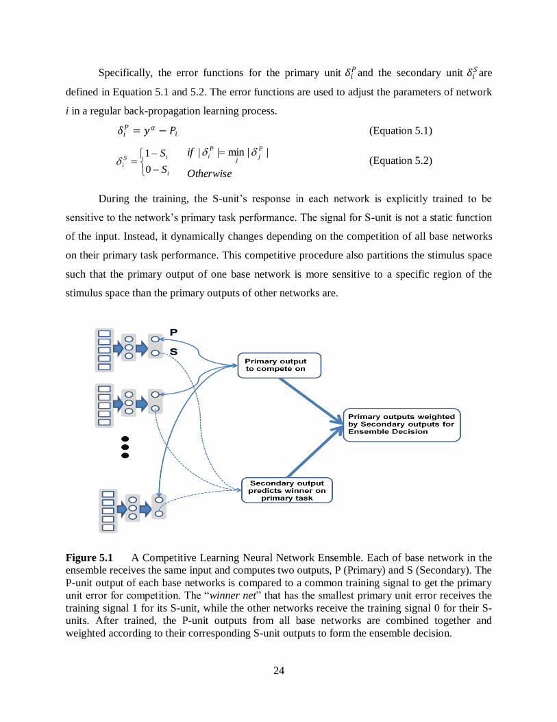
During the training, the S-unit’s response in each network is explicitly trained to be

sensitive to the network’s primary task performance. The signal for S-unit is not a static function

of the input. Instead, it dynamically changes depending on the competition of all base networks

on their primary task performance. This competitive procedure also partitions the stimulus space

such that the primary output of one base network is more sensitive to a specific region of the

stimulus space than the primary outputs of other networks are.

Figure 5.1 A Competitive Learning Neural Network Ensemble. Each of base network in the

ensemble receives the same input and computes two outputs, P (Primary) and S (Secondary). The

P-unit output of each base networks is compared to a common training signal to get the primary

unit error for competition. The “winner net” that has the smallest primary unit error receives the

training signal 1 for its S-unit, while the other networks receive the training signal 0 for their S-

units. After trained, the P-unit outputs from all base networks are combined together and

weighted according to their corresponding S-unit outputs to form the ensemble decision.

25

For any data point in the input space, each base network demonstrates different

“preference” as indicated by its secondary output. Generally, the greater the secondary output is

from a network, the higher “preference” the network shows, and thus the more accurate

classification result can be expected from the network.

Therefore, the secondary outputs, once normalized, can be utilized as the weights to

combine the primary outputs from all base networks to form the ensemble decision. In this work,

the secondary output from each base network is raised to the 2nd

power and then normalized as

shown in Equation 5.3. Previous studies [20, 67, 88] have shown that when the members in an

ensemble are imbalanced, an optimal set of weights could significantly improve the ensemble

performance.

𝜱𝑷 = 𝑷𝒊 ∗𝑺𝒊𝟐

𝑺𝒋𝟐𝑳

𝒋=𝟏 𝑳

𝒊=𝟏 (Equation 5.3)

where ΦP is the classification output of an ensemble of L base networks.

26

Chapter 6

Evaluation and Experiment Design

In the Competitive Learning Neural Network Ensemble, the base networks compete

against each other on the classification performance for every training data point. This

competitive procedure divides the input space, and decomposes the overall complex task into

smaller and easier sub-tasks. Each base network develops “preferences” over different regions of

the input space, corresponding to different sub-tasks. Such “preference” is indicated by each base

network’s secondary output. A greater secondary output shows a higher “preference” or more

accurate classification result from the base network to be expected. Therefore when the primary

outputs from all base networks are combined and weighted by their secondary outputs, the

competitive learning ensemble can usually achieve higher classification performance than a

traditional ensemble does.

6.1 The Baseline

To evaluate the performance of the proposed approach, the competitive learning

ensemble is compared to an existing ensemble method. This is to ensure a fair evaluation as the

simulation setting, algorithm parameters, and network configurations can be controlled and

maintained same in both types of ensembles.

The most popular traditional ensemble method is bagging, where each base network is

trained on a random bootstrap sample drawn from the complete training set. When combining

the outputs from all base nets, simple averaging is used to obtain the bagging ensemble output.

With each network trained on a different bootstrap sample, a bagging ensemble can effectively

gain diversity and usually outperform a single network in classification tasks. Previous studies

[11, 12, 13, 14, 15, 90] has shown bagging, as a practical and effective ensemble approach,

usually generates reasonably good classification results. In this work, the bagging ensemble is

used as the baseline classifier to be compared with the competitive learning ensemble.

27

6.2 The Datasets

Synthetic data has many advantages over real-world data when it is used to evaluate a

new approach. With synthetic data, the nature of the task, input features, dimensionality,

sampling size, and the degree of noise can be fully controlled. More importantly, 2-D synthetic

data makes it possible to visualize the effect of the new approach on how it solves the problem.

Four synthetic datasets are designed in this work, including the annulus problem, the

checkerboard problem, the 10-D parity problem, and the synthetic diabetes problem. In addition,

a real-world dataset on SPECT heart image diagnosis from the UC Irvine machine learning

repository [87] is also adopted.

6.3 Evaluation of the Ensemble Classification Error

The competitive learning ensemble can improve classification performance by effectively

decomposing the overall task into smaller sub-tasks and assigning appropriate weights to base

networks based on their “preference”. The classification performance is measured by a

classifier’s misclassification rate on the test dataset, and is compared between the competitive

learning ensemble and the traditional bagging ensemble.

6.4 Evaluation of the Secondary Unit Performance

In the competitive learning ensemble, the secondary unit of a base network is trained to

predict the network’s primary unit performance. Given an input data point, a base network with

higher secondary output is expected to have lower primary task error. The secondary outputs

serve an important role as the weights in combining the primary outputs from all base networks

to form the ensemble decision. Therefore, it is necessary to examine the relationship between the

secondary output and the primary unit error of each base network.

A scatter plot of the expected primary unit error at different levels of secondary outputs

can help visualize the trend between the two variables. For any secondary output value, the

expected primary unit error can be calculated as the average misclassification error from all base

networks on all data points where the networks’ secondary outputs are greater than the specified

secondary output value.

28

6.5 Evaluation of the Ensemble Diversity

Diversity is a very important factor for ensembles. The higher diversity an ensemble has,

the more likely its base networks make different errors, and the better ensemble classification

performance can be expected. The bagging ensemble gains diversity implicitly by randomizing

the training samples. The competitive learning ensemble, however, explicitly promotes diversity

by assigning different tasks to the secondary output unit of each base network. In each training

iteration, a particular base network is identified as the “winner network”. The “winner network”

receives a different training signal (1) from what other networks receive (0) for the secondary

output units. These different secondary tasks can in turn influence the primary task learning in

each base network through the same hidden layer units shared by both tasks.

Various measures of diversity have been studied by researchers [14, 15, 78], which is

beyond the scope of this work. The “diversity” in this study is measured by the variance of the

primary outputs from all base networks in an ensemble. Specifically, for an ensemble of L base

networks, the diversity is calculated as the variance of primary outputs from all base networks

shown in Equation 6.1:

L

i

ii xfExfEL

Diversity1

2)))(()((1

(Equation 6.1)

6.6 Evaluation of the Classification Error Decomposition

As discussed in chapter 2, regular ensembles, such as bagging, can reduce classification

error through reducing the variance component. Similarly it is expected that a competitive

learning ensemble is able to reduce the variance error component as a bagging ensemble does.

More importantly, a competitive learning ensemble may also reduce the bias component of the

classification error. This can be achieved through dividing the input space and assigning

appropriate weights to base networks based on the “preference” they show on different input data

points.

29

To estimate the bias and variance component of the classification error, twenty trials of

both types of ensembles are trained, each using a random sample drawn from the entire input

space of the classification problem.

With each training set Ti, an ensemble classifier f(x: T

i) is trained. Given the twenty

ensemble classifiers f(x: T1), … , f(x: T

20), let 𝑓 𝑥 be the average output of the twenty

ensemble classifiers on a test data point x: 𝑓 𝑥 =1

20 𝑓(𝑥; 𝑇𝑖)20

𝑖=1 . The bias and variance

component can then be estimated using the following formulas:

𝐵𝑖𝑎𝑠 𝑥 ≈ (𝑓 𝑥 − 𝐸 𝑦 𝑥 )2 (Equation 6.2)

𝑉𝑎𝑟𝑖𝑎𝑛𝑐𝑒(𝑥) ≈1

20 [𝑓 𝑥; 𝑇 𝑖 − 𝑓 𝑥 ]220

𝑖=1 (Equation 6.3)

Such bias and variance is calculated and averaged over all test data points to obtain the average

bias and average variance for both the competitive learning ensembles and the bagging

ensembles.

30

Chapter 7

Experiment Results and Discussion

The competitive learning ensemble is evaluated and compared with the traditional

bagging ensemble on five classification problems. These include the annulus problem, the

checkerboard problem, the 10-D parity problem, the synthetic diabetes problem, and the SPECT

heart problem. The first four problems are artificially designed while the last one uses a real-

world dataset. The full experiment results are shown and discussed in this chapter.

7.1 The Experiment on the 2-D Annulus Classification Problem

To illustrate the strength of the competitive learning ensemble, an artificial classification

task on a 2-Dimension input space is designed to visualize how the competitive procedure

partitions the input space. Consider a classification task of two classes in the 2-D input space

shown in Figure 7.1. All the data points falling in the annulus area between the two circles are

labeled “1”, while all the other data points are labeled “0”. Each data point consists of two input

variables x=[x1, x2]. The range of possible values of both input variables is between 0 and 1. The

two circles have the same origin point at (0.5, 0.5), with a radius of 0.5 for the outer circle and

0.3 for the inner circle. This makes the annulus area around half of the entire input space area,

and the two classes are equally distributed. More specifically, the classification function is:

0

1)(xy

Otherwise

xxandxxif 22

2

2

1

22

2

2

1 5.0)5.0()5.0(3.0)5.0()5.0( (Eq. 7.1.1)

A noisy version of this classification task can be built by introducing Gaussian noise

along the solution boundary (the two circles in this problem). Let z be a vector of random

numbers drawn from a Gaussian distribution with standard deviation s. The classification

function with noise is:

0

1)(xy

Otherwise

zxxandzxxif 22

2

2

1

22

2

2

1 )5.0()5.0()5.0()3.0()5.0()5.0(

(Eq. 7.1.2)

31

The vector z is drawn from the positive half side of the Gaussian distribution. Normalized to an

area of 1, the probability density function of z is:

esz

szP

2/)/( 2

2

2)(

(Eq. 7.1.3)

The expected value of noise z is thus calculated as:

0

/2*)(*][ szPzzE

(Eq. 7.1.4)

In this work, two levels of Gaussian noise were introduced with standard deviation 0.02

and 0.1. The expected value of the noise would be 0.016 and 0.08 respectively.

7.1.1 Illustration of the Annulus Datasets

The three variants of the annulus datasets (clean, small noise, and large noise) are

illustrated with their target classification boundaries in Figure 7.1 through 7.3. In each case, 250

data points are randomly sampled from the entire input space for the experiment. 200 data points

are used for training and the other 50 are reserved as the test set. The illustration for the entire

input space is on the left, and the sample data points are shown on the right. As shown in the

figures, the noise is introduced in a way that more noise exists closer to the solution boundary

while less noise exists further away from the boundary.

Figure 7.1 Illustration of the annulus task with no noise. The complete input space is on the

left and the sample data graph is on the right. The two circles represent the target boundaries

with radius 0.5 for the outer circle and 0.3 for the inner circle.

32

Figure 7.2 Illustration of the annulus task with small noise. The entire input space is on the


with radius 0.484 (e.g. 0.5-0.016) for the outer circle and 0.284 (e.g. 0.3-0.016) for the inner

circle.

Figure 7.3 Illustration of the annulus task with large noise. The entire input space is on the


with radius 0.42 (e.g. 0.5-0.08) for the outer circle and 0.22 (e.g. 0.3-0.08) for the inner circle.

33

7.1.2 Experiment Implementations

To evaluate the proposed approach against the baseline, 20 trials of the competitive

learning ensembles and the bagging ensembles are implemented and simulated for each of the

clean and noisy annulus tasks. Each ensemble trial is trained for 200,000 iterations on the

training set and then its generalization performance is measured on the test set. Note for the two

noisy annulus tasks, the test sets use the noiseless data with real target boundaries as illustrated

in Figure 7.2 and 7.3. This is to accurately assess the classifiers’ accuracies as discussed in [77].

Both the competitive learning ensemble and the bagging ensemble contain 5 base neural

networks. Each network has 20 hidden units. The various network parameters, such as initial

weights range, learning rates, etc are fine tuned before simulation and remain the same for both

types of ensembles.

7.1.3 Evaluation of the Misclassification Performance

The classification error distributions from the 20 trials of the competitive learning

ensembles and the bagging ensembles for each of the clean and noisy annulus tasks are shown in

the boxplots of Figure 7.4 through 7.6. Generally the competitive learning ensembles outperform

the bagging ensembles in all three cases. In the clean annulus task, the competitive learning

ensemble reduces the average misclassification error to 0.04 from 0.09 in the bagging ensembles.

Figure 7.4 Misclassification comparison – no noise

34

When the data gets noisier, the classification performance from both ensembles decreases as

expected. The competitive learning ensemble still achieves more desirable performance than the

bagging ensemble does. The average misclassification error is 0.07 (competitive) vs. 0.13

(bagging) under smaller Gaussian noise; and 0.17 (competitive) vs. 0.24 (bagging) under larger

Gaussian noise. The gain of the competitive learning ensemble over bagging ensemble is

observed decreasing when more noise is introduced into the data. This is mainly because the

competitive learning ensemble’s ability to divide input space is impacted by the presence of

noise in the dataset.

Figure 7.5 Misclassification comparison – small noise

Figure 7.6 Misclassification comparison – large noise

35

7.1.4 Visualization of the Network Preference Map

The competitive learning ensemble is able to learn the complex pattern with limited

training resources because it divides the input space and drives each base network to find its

“preference” region through competition. The secondary unit of each base network is trained to

indicate if a network “prefers” a given data point. After trained, given a data point in the input

space, the higher the secondary output is, the more “preference” the base network shows on the

data point, and thus the higher weight this network is assigned for the ensemble decision. When

the input space is appropriately divided through the competition procedure, the overall complex

task is decomposed into smaller sub-tasks that are easier to tackle.

The Network Preference Map assigns the "winner networks" (coded by color) over the

entire input space. The network inputs are drawn from a uniform sample of the unit square with

resolution 0.01. Each region shows the portion of the input space for which a specific network

has the highest secondary unit response. Figure 7.7 through 7.9 illustrates the Network

Preference Map in each of the clean and noisy annulus datasets. The two circles in each figure

represent the solution boundaries. Note the boundary lines that separate the “preference” regions

for each base network show alignments with the two circles in some area.

Figure 7.7 Network Preference Map – no noise

36

Figure 7.8 Network Preference Map – small noise

Figure 7.9 Network Preference Map – large noise

7.1.5 Visualization of the Ensemble Outputs and the ROC Curves

The output from a neural network ensemble in this experiment is a continuous value

between 0 and 1. With a classification threshold, such as 0.5, an ensemble output can be

classified to be either “inside annulus” (output>=0.5) or “outside annulus” (output<0.5). One

way to illustrate the impact of noise is to visualize these ensemble outputs on the entire 2-D input

space. This shows what an ensemble thinks the annulus should look like in the clean and noisy

annulus tasks. In this experiment, an ensemble is trained on the clean and noisy data, and applied

on the data points uniformly drawn from the entire input space with resolution 0.01.

37

Figure 7.10 Competitive learning ensemble output (threshold 0.5) – no noise

Figure 7.11 Competitive learning ensemble output (threshold 0.5) - small noise

Figure 7.12 Competitive learning ensemble output (threshold 0.5) -large noise

38

Figure 7.10 through 7.12 illustrates the competitive learning ensemble outputs in the

clean, small noise and large noise cases with the classification threshold 0.5. The two circles in

each figure represent the solution boundaries. The ensemble outputs well resemble the target

annulus for the clean and small noise cases, but there exist significant false positive errors for the

large noise case. Such false positive errors can be reduced by fine tuning the classification

threshold for ensemble outputs. Table 7.1 summaries the false positive (FP) and false negative

(FN) tradeoff for different thresholds in the large noise case. And the ROC curve is shown in

Figure 7.13.

Table 7.1 The type I and type II errors by classification thresholds

Classification

Threshold Type1

(FP) Type2

(FN) True

Positive

0.06 100.0% 0.0% 100.0% 0.10 91.3% 0.0% 100.0% 0.20 82.4% 0.1% 99.9% 0.30 77.2% 0.1% 99.8% 0.40 73.6% 0.2% 99.7% 0.50 65.3% 0.4% 99.5% 0.60 58.5% 0.5% 99.2% 0.70 52.3% 0.6% 99.0% 0.80 45.5% 1.0% 98.4% 0.90 34.7% 2.2% 96.6% 0.95 21.4% 12.1% 81.3% 0.99 7.8% 44.9% 30.6% 1.00 0.00 0.65 0.00

Figure 7.13 The ROC curve for the large noise annulus task

Th=0.7Th=0.9

Th=0.95

0.0

0.2

0.4

0.6

0.8

1.0

0.0 0.2 0.4 0.6 0.8 1.0

Tru

e P

osi

tive

Rat

e

False Positive Rate

ROC for Annulus - Large Noise

39

The Figure 7.14 through 7.16 show the competitive learning ensemble output plots under

the three thresholds (0.7, 0.9 and 0.95) where the ensemble outputs are reasonably aligned with

the solution boundaries. These three thresholds are also labeled in red in the ROC curve.

Figure 7.14 Competitive learning ensemble output (threshold 0.7) – large noise



40

The Figure 7.17 shows the ROC curve comparison for the clean, small noise and large

noise annulus tasks. The areas under the three ROC curves illustrate the competitive learning

ensemble’s ability to correctly classify the task under different noise level. These areas can be

approximated with a non-parametric method based on constructing trapezoids under the ROC

curve. The Figure 7.18 shows the comparison of the areas under the three ROC curves. The area

decreases as the noise level increases in the annulus task.

Figure 7.17 The ROC curve for the annulus tasks – clean, small noise and large noise

Figure 7.18 The ROC area for the annulus tasks – clean, small noise and large noise

0.00

0.10

0.20

0.30

0.40

0.50

0.60

0.70

0.80

0.90

1.00

0.00 0.20 0.40 0.60 0.80 1.00

Tru

e P

osi

tive

Rat

e

False Positive Rate

ROC Curve for Annulus - All Tasks

Clean

Small Noise

Large Noise

0.950.93

0.85

0.50

0.60

0.70

0.80

0.90

1.00

Clean Small Noise Large Noise

ROC Area for Annulus - All Tasks

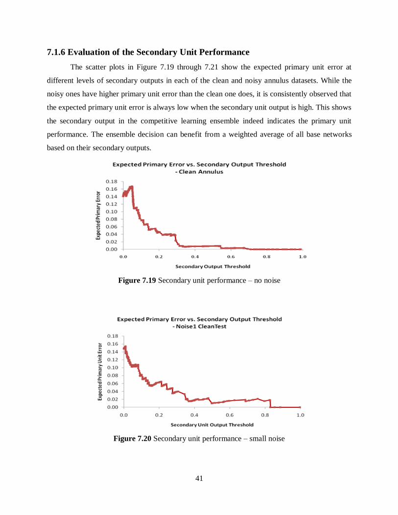
41

7.1.6 Evaluation of the Secondary Unit Performance

The scatter plots in Figure 7.19 through 7.21 show the expected primary unit error at

different levels of secondary outputs in each of the clean and noisy annulus datasets. While the

noisy ones have higher primary unit error than the clean one does, it is consistently observed that

the expected primary unit error is always low when the secondary unit output is high. This shows

the secondary output in the competitive learning ensemble indeed indicates the primary unit

performance. The ensemble decision can benefit from a weighted average of all base networks

based on their secondary outputs.

Figure 7.19 Secondary unit performance – no noise

Figure 7.20 Secondary unit performance – small noise

42

Figure 7.21 Secondary unit performance – large noise

7.1.7 Evaluation of the Ensemble Diversity

To compare the diversity between the two types of ensembles, twenty trials of the

competitive learning ensembles and the bagging ensembles are implemented and tested on the

clean annulus task. The distributions of their diversity are shown in Figure 7.22, where the

competitive learning ensemble is observed to have greater diversity than the bagging ensemble

does.

Figure 7.22 Diversity comparison for the annulus task

43

7.1.8 Evaluation of the Classification Error Decomposition

As discussed in the previous chapters, classification error can be decomposed into

variance component and bias component. Regular ensembles such as bagging can improve

classification performance mainly through reducing the variance component. However the

competitive learning ensembles can also reduce the bias error component through dividing input

space and assigning appropriate weights based on network preference.

Figure 7.23 and Figure 7.24 illustrate the bias and variance classification error

decomposition in the clean annulus task for both the competitive learning ensemble and the

bagging ensemble. The competitive learning ensemble has shown much smaller bias error than

the bagging ensemble does. Note the variance error component in the competitive learning

ensemble is also smaller than that in the bagging ensemble. This is because each competitive

learning ensemble is more accurate and closer to the target, and thus achieves smaller variance

among the ensemble results.

Figure 7.23 Classification error decomposition - bias

Figure 7.24 Classification error decomposition - variance

0.02

0.04

0.000

0.010

0.020

0.030

0.040

Competitive Learning Bagging

Classification Error Decomposition - Bias

0.02

0.03

0.000

0.005

0.010

0.015

0.020

0.025

0.030

0.035

Competitive Learning Bagging

Classification Error Decomposition - Variance

44

7.2 The Experiment on the Checkerboard Classification Problem

Consider a classification problem with two classes shown in Figure 7.25. There are 49

data points arranged on a 7x7 checkerboard matrix with alternating categorical values of 1 (25

data points) and 0 (24 data points). Each data point consists of two input features: the horizontal

and vertical coordinate values in the range between 0 and 1.

Figure 7.25 The checkerboard problem

This classification task is a non-trivial task as the data points from different classes are

close to each other. As illustrated in Figure 7.26, this classification task may be solved with

multiple boundary lines parallel to the matrix diagonal. The input space is then divided into 13

sub-regions, each containing either all 1’s or all 0’s.

45

Figure 7.26 A solution to the checkerboard problem

In this work, 7 data points (3 1’s and 4 0’s) are picked as the test set, and the other 42

data points (22 1’s and 20 0’s) are used as the training set. A classifier is expected to learn the

separation boundaries from the training set and generalize to the test set. The test data points are

uniformly distributed, as marked with red circles in Figure 7.27. The minimal distance between

test data points is 2 units on the grid, and the nearest pairs of test data points are in different

classes.

Figure 7.27 The experiment setup for the checkerboard problem

46



learning ensembles and the bagging ensembles are implemented. Each ensemble trial is trained

for 100,000 iterations on the training set and then its generalization performance is measured on

the test set. Both the competitive learning ensemble and the bagging ensemble contain 5 base

neural networks. Each network has 20 hidden units. The various network parameters, such as

initial weights range, learning rates, etc are fine tuned before simulation and remain the same for

both types of ensembles.

In the bagging ensembles, a random bootstrap sample is retrieved from the training set to

train each base network in the experiment. Due to the limited size of the training set, the bagging

approach may not show significant performance improvement over single neural networks.

In the competition learning ensembles, each base network in the ensemble processes the

same data point retrieved from the training set in each training iteration. The base network that

has the smallest classification error for the data point is identified as the “winner net”, and

receives signal 1 for its secondary unit; while the other networks receive 0 for their secondary

units in the training iteration. The primary units of all base networks receive the same training

single for the classification task.

7.2.2 Performance Evaluation

The error distributions from 20 trials of the competitive learning ensembles and the

bagging ensembles are compared in the boxplot in Figure 7.28. The bagging ensembles are not

learning the patterns well with an average misclassification rate of 0.4. On the other hand, the

competitive leaning ensembles have effectively solved the problem and successfully generalize

on the test set with the same number of hidden units and training iterations. The competitive

learning ensemble reduces the misclassification error to 0.23.

47

Figure 7.28 Misclassification comparison for the checkerboard problem

The Network Preference Map in Figure 7.29 assigns the "winner networks" (coded by

color) over the entire input space. Each region shows the part of the input space for which a

specific network has the highest secondary unit response. The boundary lines in the graph that

separate the “preference” regions for each base network resemble the solution boundary lines

shown in Figure 7.26. This indicates the competitive learning ensemble effectively divides the

input space, and thus decomposes an overall complex task into smaller and easier tasks.

It is also interesting to visualize the ensemble outputs and find what the ensemble thinks

the solution boundaries are. Figure 7.30 shows the outputs from a competitive learning ensemble.

The network inputs are uniformly drawn from the entire input space with resolution 0.01. The

solution boundaries calculated by the ensemble are well aligned with the target boundary lines

shown in Figure 7.26, except on the lower right corner.

48

Figure 7.29 The Network Preference Map for the checkerboard problem. Network inputs are

drawn from a uniform sample of the unit square with resolution 0.01. The color corresponds to

the base network with the highest secondary unit response. The 49 data points of the

classification task are overlaid onto the Network Preference Map showing the patterns in sub-

regions are much simpler than the overall task.

Figure 7.30 The ensemble output for the checkerboard problem. Network inputs are drawn

from a uniform sample of the unit square with resolution 0.01. The 49 data points of the

classification task are overlaid onto the ensemble output graph.

49

To examine the secondary unit performance of the competitive learning ensemble, a

scatter plot of the expected primary unit error at different levels of secondary outputs is shown in

Figure 7.31. It is again observed that the expected primary unit error is always low when the

secondary output is high. This shows the secondary output in the competitive learning ensemble

indeed indicates the primary unit performance.

Figure 7.31 Secondary unit performance for the checkerboard problem

The diversity comparison between the two types of ensembles is shown in Figure 7.32,

where the competitive learning ensembles are observed to have greater diversity than the

bagging ensembles do.

Figure 7.32 Diversity comparison for the checkerboard problem

0

0.1

0.2

0.3

0.4

0 0.2 0.4 0.6 0.8 1

Exp

ecte

d P

rim

ary

Un

it E

rro

r

Secondary Unit Output Threshold

Expected Primary Error vs. Secondary Output Threshold

50

7.3 The Experiment on the 10-D Parity Classification Problem

The 10-D parity task is to classify a sequence of 10 binary digits to either 1 or 0

depending on its number of 1’s is odd or even. The target class is 1 for odd and 0 for even. The

entire input space contains 1024 (210

) data points. The cases of class 1’s and 0’s are equally

distributed over the input space.



learning ensembles and the bagging ensembles are implemented. In each simulation, 800 data

points are randomly drawn for the training set and the rest 224 are reserved as the test set. Each

ensemble trial is trained for 200,000 iterations on the training set and then its generalization

performance is measured on the test set.




types of ensembles.


The error distributions from 20 trials of the competitive learning ensembles and the

bagging ensembles are compared in the boxplot in Figure 7.33. The competitive learning

ensembles are shown outperforming the bagging ensembles, and reducing the average

misclassification error to 0.08 from 0.14.

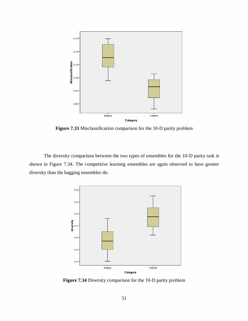
51

Figure 7.33 Misclassification comparison for the 10-D parity problem

The diversity comparison between the two types of ensembles for the 10-D parity task is

shown in Figure 7.34. The competitive learning ensembles are again observed to have greater

diversity than the bagging ensembles do.

Figure 7.34 Diversity comparison for the 10-D parity problem

52

7.3.3 The Distribution of “Winner Networks”

By the nature of the competitive learning ensemble, any input data point can be

associated with a particular “winner network” that has the highest secondary unit response

among all base networks. It is interesting to analyze the distribution of the “winner networks”

and how the entire input space is divided by each base network. The data points “preferred” by

the same “winner networks” tend to be closer to each other compared to the data points

“preferred” by different “winner networks”. For the 10-D parity task, it is challenging to

visualize such distribution through the Network Preference Map shown in previous chapters.

However it can be estimated by examining the pair-wise distance among all data points in the

input space. In this experiment, the distance is measured by the Euclidean distance.

Table 7.2 summarizes such pair-wise distance matrix. The highlighted cells are the

average pair-wise distance of data points “preferred” by the same “winner networks”, while the

un-highlighted cells are the average pair-wise distance of data points “preferred” by different

“winner networks”. As an example, the average pair-wise distance of data points “preferred” by

network0 is 1.95; while the average pair-wise distance between data points “preferred” by

network0 and network1 is 2.24. Table 7.3 further illustrates the detailed cumulative percentage

distribution of the pair-wise distance “preferred” by the same and different “winner networks”.

Generally the average pair-wise distance of data points from the same “winner networks”

is smaller than the average pair-wise distance of those from different “winner networks” as

shown in Table 7.2. More specifically, picking 2.0 as a threshold for small distances, Table 7.3

shows 48% of the distances from the same “winner networks” are small distances; while only 37%

of the distances from different “winner networks” are small distances. Note the data points

“preferred” by the same “winner networks” could possibly spread over the input space in the

form of several small chunks. The pair-wise distance analysis only reveals the overall pattern

that data points “preferred” by the same “winner networks” are more likely to be close together

than data points “preferred” by different “winner networks” are.

53

Table 7.2 The pair-wise distance matrix for the 10-D parity problem

Pair-wise Dist Net0 Net1 Net2 Net3 Net4 Net0 1.95 2.24 2.24 2.17 2.26 Net1

2.15 2.18 2.24 2.24

Net2

2.17 2.23 2.21 Net3

2.18 2.20

Net4

2.18

Table 7.3 The cumulative percentage by pair-wise distance for the 10-D parity problem

Distance Threshold

Net0 Net1 Net2 Net3 Net4 Average

<=0.5 0% 0% 0% 0% 0% 0% <=1 2% 1% 1% 1% 1% 1%

<=1.5 16% 10% 9% 6% 6% 10% <=2 71% 44% 46% 40% 40% 48%

<=2.5 97% 89% 87% 84% 85% 88% <=3 100% 100% 99% 100% 100% 100%

More 100% 100% 100% 100% 100% 100%

Distance Threshold

N0-N1 N0-N2 N0-N3 N0-N4 N1-N2 N1-N3 N1-N4 N2-N3 N2-N4 N3-N4 Average

<=0.5 0% 0% 0% 0% 0% 0% 0% 0% 0% 0% 0% <=1 1% 1% 2% 1% 0% 1% 1% 1% 1% 1% 1%

<=1.5 5% 4% 6% 4% 7% 4% 4% 4% 4% 6% 5% <=2 35% 33% 40% 34% 48% 34% 33% 36% 37% 38% 37%

<=2.5 75% 76% 86% 78% 85% 81% 80% 81% 82% 83% 81% <=3 100% 100% 100% 100% 100% 100% 100% 100% 100% 100% 100%

More 100% 100% 100% 100% 100% 100% 100% 100% 100% 100% 100%

Figure 7.35 shows the histograms to compare the distances of data points “preferred” by

the same and different “winner networks” for each base network in the competitive learning

ensemble. The blue bars show the distance distribution from the data points of the same “winner

networks” while the red bars show that from the data points of different “winner networks”. Note

when the distances are small (less than 2.0), the blue bars are higher indicating a bigger portion

of distances from the same “winner networks” are small. The detailed histograms for distances

from the same and different “winner networks” are shown in Figure 7.36 and 7.37, where the

same patterns are observed.

54

Figure 7.35 Distance histograms - by “Winner Networks”

0%

10%

20%

30%

40%

50%

60%

0.5 1 1.5 2 2.5 3

WinNet 0 Distance Distribution

Same WinNet

Different WinNet

0%

10%

20%

30%

40%

50%

0.5 1 1.5 2 2.5 3


Same WinNet

Different WinNet

0%

10%

20%

30%

40%

50%

0.5 1 1.5 2 2.5 3


Same WinNet

Different WinNet

0%

10%

20%

30%

40%

50%

0.5 1 1.5 2 2.5 3


Same WinNet

Different WinNet

0%

10%

20%

30%

40%

50%

0.5 1 1.5 2 2.5 3


Same WinNet

Different WinNet

55

Figure 7.36 Distance histograms - by the same “Winner Networks”

0.00%

50.00%

100.00%

0

50

100

150

200

0.5 1 1.5 2 2.5 3

Fre

qu

en

cy

Bin

WinNet 0 Histogram

0.00%

50.00%

100.00%

0

20

40

60

80

0.5 1 1.5 2 2.5 3

Fre

qu

en

cy

Bin

WinNet 1 Histogram

0.00%20.00%40.00%60.00%80.00%100.00%

0

20

40

60

0.5 1 1.5 2 2.5 3

Fre

qu

en

cy

Bin

WinNet 2 Histogram

0.00%20.00%40.00%60.00%80.00%100.00%

0

1000

2000

3000

0.5 1 1.5 2 2.5 3Fr

eq

ue

ncy

Bin

WinNet 3 Histogram

0.00%

50.00%

100.00%

0

200

400

600

800

0.5 1 1.5 2 2.5 3

Fre

qu

ency

Bin

WinNet4 Histogram

0.00%20.00%40.00%60.00%80.00%100.00%

0

20

40

60

80

0.5 1 1.5 2 2.5 3

Fre

qu

ency

Bin

WinNet N0-N1 Histogram

0.00%20.00%40.00%60.00%80.00%100.00%

0

20

40

60

80

0.5 1 1.5 2 2.5 3

Fre

qu

ency

Bin


56

Figure 7.37 Distance histograms - by different “Winner Networks”

0.00%

50.00%

100.00%

0

500

1000

1500

0.5 1 1.5 2 2.5 3

Fre

qu

en

cy

Bin


0.00%

50.00%

100.00%

0

200

400

600

0.5 1 1.5 2 2.5 3

Fre

qu

en

cy

Bin


0.00%

20.00%

40.00%

60.00%

80.00%

100.00%

0

20

40

60

0.5 1 1.5 2 2.5 3

Fre

qu

en

cy

Bin


0.00%

20.00%

40.00%

60.00%

80.00%

100.00%

0

200

400

600

800

1000

0.5 1 1.5 2 2.5 3Fr

eq

ue

ncy

Bin


0.00%20.00%40.00%60.00%80.00%100.00%

0100200300400500

0.5 1 1.5 2 2.5 3

Fre

qu

ency

Bin


0.00%

50.00%

100.00%

0

200

400

600

800

0.5 1 1.5 2 2.5 3

Fre

qu

ency

Bin


0.00%

50.00%

100.00%

0100200300400

0.5 1 1.5 2 2.5 3

Fre

qu

ency

Bin


0.00%

50.00%

100.00%

0200400600800

0.5 1 1.5 2 2.5 3

Fre

qu

en

cy

Bin


57

7.4 The Experiment on the Synthetic Diabetes Problem

The synthetic diabetes data is built based on the Pima Indians Diabetes Dataset in the

UCI machine learning repository [87]. The original dataset contains the diagnoses of 768 female

patients who are at least 21 years old of Pima Indian heritage based on the following 8 attributes:

1. Number of times pregnant

2. Plasma glucose concentration a 2 hours in an oral glucose tolerance test

3. Diastolic blood pressure (mm Hg)

4. Triceps skin fold thickness (mm)

5. 2-Hour serum insulin (mu U/ml)

6. Body mass index (weight in kg/(height in m)^2)

7. Diabetes pedigree function

8. Age (years)

The synthetic diabetes data is designed to imitate the Pima Indians Diabetes Dataset so

the distribution of the input features and the pair-wise correlation among input features from the

original dataset are preserved in the synthetic dataset. The detailed procedures to develop the

synthetic dataset are as follows:

1. Calculate the pair-wise correlation matrix from the original Pima Indians Diabetes

Dataset.

2. Calculate the mean and standard deviation of each input feature from the original

Pima Indians Diabetes Dataset.

3. Generate synthetic random data with the target pair-wise correlation from step 1 using

the technique at [99].

4. Rescale the synthetic data with the target mean and standard deviation for each input

feature from step 2.

5. Train a single neural network classifier on the original Pima Indians Diabetes Dataset,

and apply the trained network classifier on the synthetic dataset from step 4. For each

input data point, the neural network classifier generates a continuous value between 0

and 1. Use the threshold 0.5 to categorize the data point to class 1 or 0.

6. Choose 5% data points near the solution boundary to flip their target class from 1 to 0

or from 0 to 1. The boundary data points are those whose neural network outputs are

the closest to the classification threshold 0.5.

58

The synthetic dataset contains 500 data points in total. A comparison between the

correlation matrix from the original dataset (Table 7.4) and that from the synthetic dataset (Table

7.5) shows the pair-wise correlation from original input space has been well preserved.

Table 7.4 The correlation matrix of the original diabetes dataset

Original X1 X2 X3 X4 X5 X6 X7 X8

X1 1.00 0.13 0.14 -0.08 -0.07 0.02 -0.03 0.54 X2 0.13 1.00 0.15 0.06 0.33 0.22 0.14 0.26 X3 0.14 0.15 1.00 0.21 0.09 0.28 0.04 0.24 X4 -0.08 0.06 0.21 1.00 0.44 0.39 0.18 -0.11 X5 -0.07 0.33 0.09 0.44 1.00 0.20 0.19 -0.04 X6 0.02 0.22 0.28 0.39 0.20 1.00 0.14 0.04 X7 -0.03 0.14 0.04 0.18 0.19 0.14 1.00 0.03 X8 0.54 0.26 0.24 -0.11 -0.04 0.04 0.03 1.00

Table 7.5 The correlation matrix of the synthetic diabetes dataset

Synthetic X1 X2 X3 X4 X5 X6 X7 X8

X1 1.00 0.14 0.10 -0.11 -0.05 -0.02 0.00 0.57 X2 0.14 1.00 0.16 0.10 0.33 0.27 0.04 0.25 X3 0.10 0.16 1.00 0.26 0.04 0.38 -0.05 0.18 X4 -0.11 0.10 0.26 1.00 0.43 0.46 0.16 -0.16 X5 -0.05 0.33 0.04 0.43 1.00 0.24 0.17 0.02 X6 -0.02 0.27 0.38 0.46 0.24 1.00 0.12 0.00 X7 0.00 0.04 -0.05 0.16 0.17 0.12 1.00 0.05 X8 0.57 0.25 0.18 -0.16 0.02 0.00 0.05 1.00

To compare the distribution of each input feature between the original data and the

synthetic data, their histograms are plotted side by side in Figure 7.38. It’s shown that most input

features from the synthetic data have similar distribution to their counterparts in the original data,

but some (e.g. X2, X3, X4 in synthetic data) are a little skewed towards Gaussian distribution.

59

Input Variable 1: Number of times pregnant

Input Variable 2: Plasma glucose concentration a 2 hours in an oral glucose tolerance test

Input Variable 3: Diastolic blood pressure (mm Hg)

Input Variable 4: Triceps skin fold thickness (mm)

0.0%

10.0%

20.0%

30.0%

40.0%

1 2 3 4 5 More

Original Data - X1

0.0%

10.0%

20.0%

30.0%

40.0%

1 2 3 4 5 More

Synthetic Data - X1

0.0%

10.0%

20.0%

30.0%

40.0%

60 90 120 150 180 More

Original Data - X2

0.0%

10.0%

20.0%

30.0%

40.0%

60 90 120 150 180 More

Synthetic Data - X2

0.0%

10.0%

20.0%

30.0%

40.0%

50.0%

30 50 70 90 110 More

Original Data - X3

0.0%

10.0%

20.0%

30.0%

40.0%

50.0%

30 50 70 90 110 More

Syntehtic Data - X3

0.0%

10.0%

20.0%

30.0%

5 15 25 35 50 More

Original Data - X4

0.0%

5.0%

10.0%

15.0%

20.0%

25.0%

5 15 25 35 50 More

Synthetic Data - X4

60

Input Variable 5: 2-Hour serum insulin (mu U/ml)

Input Variable 6: Body mass index (weight in kg/(height in m)^2)

Input Variable 7: Diabetes pedigree function

Input Variable 8: Age (years)

Figure 7.38 Histogram of input variables – the original and synthetic diabetes problem

0.0%

20.0%

40.0%

60.0%

10 30 75 100 150 More

Original Data - X5

0.0%

10.0%

20.0%

30.0%

10 30 75 100 150 More

Synthetic Data - X5

0.0%

10.0%

20.0%

30.0%

40.0%

15 25 30 35 50 More

Original Data - X6

0.0%

10.0%

20.0%

30.0%

40.0%

15 25 30 35 50 More

Synthetic Data - X6

0.0%

10.0%

20.0%

30.0%

40.0%

50.0%

0.1 0.3 0.5 0.8 1 More

Original Data - X7

0.0%

10.0%

20.0%

30.0%

40.0%

0.1 0.3 0.5 0.8 1 More

Synthetic Data - X7

0.0%

10.0%

20.0%

30.0%

40.0%

25 30 40 50 60 More

Original Data - X8

0.0%

10.0%

20.0%

30.0%

40.0%

25 30 40 50 60 More

Synthetic Data - X8

61



learning ensembles and the bagging ensembles are implemented. In each simulation, 400 data

points are randomly drawn for the training set and the rest 100 are reserved as the test set. Each

ensemble is trained for 100,000 iterations on the training set and then its generalization

performance is measured on the test set.




types of ensembles.


The error distributions from the competitive learning ensembles, the bagging ensembles,

and the base networks in both types of the ensembles are compared in Figure 7.39. In general,

both ensemble approaches decrease the classification error over the base networks. The

competitive learning ensembles further outperform the bagging ensembles, and reduce the

average misclassification error to 0.10 from 0.14. Notice the base networks in the competitive

learning ensembles perform a little worse than those in the bagging ensembles do. This is mainly

because of the secondary task introduced to the base networks in the competitive learning

ensembles. Even when its base network performance is slightly degraded, the competitive

learning ensemble performance can be enhanced by effectively dividing input space and

assigning appropriate weights to base networks based on their “preference”.

Figure 7.40 shows the diversity comparison between the two types of ensembles for the

synthetic diabetes task. The competitive learning ensembles are again observed to have greater


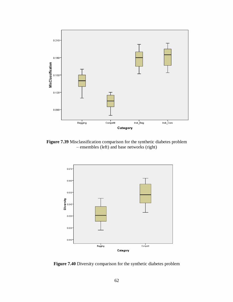
62

Figure 7.39 Misclassification comparison for the synthetic diabetes problem

– ensembles (left) and base networks (right)

Figure 7.40 Diversity comparison for the synthetic diabetes problem

63

7.5 The Experiment on the SPECT Heart Classification Problem

The SPECT heart problem from UCI machine learning repository [87] is a real-world

dataset. It describes the diagnosing of cardiac Single Proton Emission Computed Tomography

(SPECT) images. Each of the 267 images is classified into two classes: normal (0) and abnormal

(1), based on the 22 binary features extracted from the original images. The dataset has uneven

number of 1’s (21%) and 0’s (79%). With over-sampling, the training set contains 80 data points,

including 50% 1’s and 50% 0’s. The rest 187 data points are reserved as the test set.



learning ensembles and the bagging ensembles are implemented. Each ensemble trial is trained

for 200,000 iterations on the training set and then its generalization performance is measured on

the test set.




types of ensembles.


The error distributions from the competitive learning ensembles, the bagging ensembles,

and the base networks in both types of the ensembles are compared in Figure 7.41. Both

ensemble approaches are shown decreasing the classification error over the base networks. The

competitive learning ensembles further outperform the bagging ensembles, and reduce the

average misclassification error to 0.20 from 0.25. It is also observed the base networks in the

competitive learning ensembles perform a little worse than those in the bagging ensembles do, as

the result of secondary tasks introduced. However the competitive learning ensemble

performance is enhanced even when its base networks performance is slightly degraded.

The diversity comparison between the two types of ensembles for the SPECT heart task

is shown in Figure 7.42. The competitive learning ensembles are again observed to have greater


64

Figure 7.41 Misclassification comparison for the SPECT heart problem

– ensembles (left) and base networks (right)

Figure 7.42 Diversity comparison for the SPECT heart problem

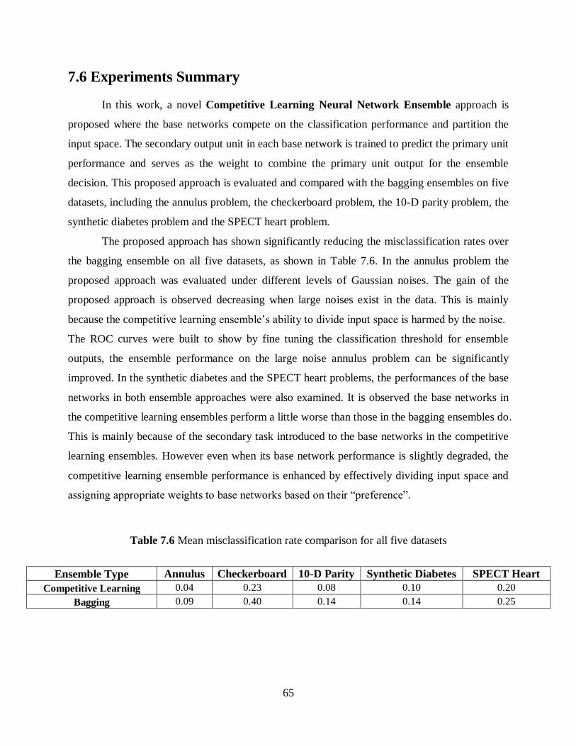
65

7.6 Experiments Summary

In this work, a novel Competitive Learning Neural Network Ensemble approach is

proposed where the base networks compete on the classification performance and partition the

input space. The secondary output unit in each base network is trained to predict the primary unit

performance and serves as the weight to combine the primary unit output for the ensemble

decision. This proposed approach is evaluated and compared with the bagging ensembles on five

datasets, including the annulus problem, the checkerboard problem, the 10-D parity problem, the

synthetic diabetes problem and the SPECT heart problem.

The proposed approach has shown significantly reducing the misclassification rates over

the bagging ensemble on all five datasets, as shown in Table 7.6. In the annulus problem the

proposed approach was evaluated under different levels of Gaussian noises. The gain of the

proposed approach is observed decreasing when large noises exist in the data. This is mainly

because the competitive learning ensemble’s ability to divide input space is harmed by the noise.

The ROC curves were built to show by fine tuning the classification threshold for ensemble

outputs, the ensemble performance on the large noise annulus problem can be significantly

improved. In the synthetic diabetes and the SPECT heart problems, the performances of the base

networks in both ensemble approaches were also examined. It is observed the base networks in

the competitive learning ensembles perform a little worse than those in the bagging ensembles do.

This is mainly because of the secondary task introduced to the base networks in the competitive

learning ensembles. However even when its base network performance is slightly degraded, the

competitive learning ensemble performance is enhanced by effectively dividing input space and

assigning appropriate weights to base networks based on their “preference”.

Table 7.6 Mean misclassification rate comparison for all five datasets

Ensemble Type Annulus Checkerboard 10-D Parity Synthetic Diabetes SPECT Heart

Competitive Learning 0.04 0.23 0.08 0.10 0.20

Bagging 0.09 0.40 0.14 0.14 0.25

66

In the proposed approach, the competitive procedure drives base networks to develop

“preference” over different region of the input space and thus decompose the overall complex

task into smaller and easier sub-tasks. The Network Preference Map was built to visualize such

input space partition for the 2-D classification problems (e.g. the annulus and the checkerboard

problems). The color regions in the map show the portions of the input space where a specific

network has the highest secondary unit response. It is observed that the boundary lines that

separate the “preference” regions for base networks show alignments with the classification

solution boundaries in some area.

The effectiveness of the proposed approach largely relies on the ability of the secondary

unit predicting the primary unit error. In the annulus and the checkerboard problems, a scatter

plot of the primary unit error versus the secondary output is built. Clear trend is observed that

when the secondary output gets higher, the expected primary unit error is always lower.

In the annulus task, the bias/variance error decomposition was examined for both

ensemble approaches. The competitive learning ensembles have shown reducing both the bias

and the variance errors, compared to the bagging ensembles. This is mainly achieved by

partitioning the input space and assigning appropriate weights based on network preference.

Lastly the ensemble diversity, as measured by the variance among base networks outputs,

for both approaches were evaluated. The competitive learning ensembles have shown

significantly higher diversity than the bagging ensembles do on all five classification problems.

With these experiments, the proposed approach has been fully evaluated on five different

aspects: misclassification error, input space partition, secondary unit performance, bias/variance

error decomposition, and the ensemble diversity. The results are consistent and have

demonstrated the strength of the competitive learning ensemble.

67

Chapter 8

Conclusion and Future Directions

The effectiveness of an ensemble approach over a single classifier has been theoretically

proven. Ensemble performance increases when the base classifiers make different errors.

Prompting diversity is critical in building ensembles. Various techniques have been explored to

optimize ensemble performance. An important characteristic of a neural network classifier is its

ability to learn multiple tasks simultaneously by simply adding an additional output unit. The

primary and secondary output units share the same hidden units and are trained simultaneously

through the back-propagation procedure. This characteristic can be utilized to develop an

effective neural network ensemble. Networks that receive different training signals for their

secondary output units tend to generalize differently on the primary task. What is more, when the

secondary unit of a network is trained to predict the primary unit performance and used as the

weights to combine base networks’ primary outputs for ensemble decision, significant

performance improvement can be achieved.

This work has proposed a Competitive Learning Neural Network Ensemble where a

secondary output unit predicts the classification performance of the primary output unit in each

base network. The networks compete with each other on the basis of classification performance

and partition the stimulus space. The secondary unit adaptively receives different training signals

depending on the competition. For any input data item fed into the ensemble, the network that

computes the minimal classification error is identified as the winner network. This winner

network receives training signal 1 for its secondary output unit, while the other networks receive

0 for their secondary output units. During the training, the secondary output unit in each base

network is explicitly trained to be sensitive to the network’s primary unit performance. The

training signals for the secondary units dynamically change for each base network when different

input data items are processed. As the result of the competition, each base network develops

“preference” over different regions of the input space as indicated by their secondary unit outputs.

Given any data point in the input space, the higher the secondary output is, the more “preference”

the network shows on the data point, and the more accurate classification result the network can

68

generate. To form an ensemble classification decision, all base networks’ primary outputs are

combined and weighted according to their secondary outputs.

With the experiments on one real-world and four artificial problems, the proposed

approach has shown outperforming the traditional bagging ensembles where each base network

is trained on a random bootstrap sample from the training set. Significant misclassification rate

reduction and higher diversity among base networks have been achieved in the proposed

approach.

The secondary units in the proposed approach accurately indicate the primary task

performance of base networks; and the ensemble decisions benefit from the weighted average

according to base networks’ secondary outputs. The scatter plots of the expected primary unit

errors at different levels of secondary outputs show the expected primary unit error is always low

when the secondary output is high.

The visualizations of Network Preference Map on the 2D datasets show the competitive

procedure can effectively partition the input space and drive base networks to different

“preference” regions over the input space as indicated by their secondary output value. The

boundary lines in the Network Preference Map often align with the target solution boundaries,

implying an overall complex task is decomposed into smaller and easier sub-tasks. However this

ability to divide the input space can be impaired by the presence of noise in datasets; thus the

benefits of the proposed approach may be reduced when significant noise exists as discussed in

the annulus problem. It is also noticeable from the Network Preference Map that the data points

“preferred” by the same “winner networks” often spread over the input space in the form of

several small chunks, rather than forming one big continuous sub-region.

The proposed approach was also evaluated from the perspective of classification error

decomposition. Classification error can be decomposed into variance and bias components. By

taking the aggregate from a group of base classifiers, regular ensembles such as bagging can

reduce the variance component of the classification error. However, the proposed approach has

also shown being able to reduce the bias error component by partitioning the input space and

assigning appropriate weights based on network preference.

Related to this work, there are some interesting research topics that can be studied in

future work. One is to optimize the aggregate funciton that combines the primary outputs from

all base networks for ensemble decision. In this work, the aggregate function is the mean of

69

primary outputs weighted by the normalized square of the secondary outputs from all base

networks. The scatter plots of the expected primary unit error versus the secondary output have

shwon when the secondary output gets higher the expected primary error is lower. Such

underlying relationship between the primary unit performance and the secondary output may

vary in different types of classification problems. That can be derived to adaptively optimize the

aggregate function for even better ensemble decision.

Another direction is to explore how to use secondary tasks to solve clustering problems.

Intuitively the competitive procedure can not only partition the input space but also generate

meaningful clusters. Data points that are “preferred” by the same network may share some

common characteristics and thus are likely to be in the same cluster. Chapter 7 shows some

distribution analysis for the “winner networks”. Just like in clusters, the distance of data points

“preferred” by the same “winner networks” tend to be smaller than the distance of data points

“preferred” by different “winner networks”. What would be the difference between this

clustering method and other clustering algorithms such as K-mean? How can the secondary tasks

be modified to generate better clustering?

Lastly, different types of secondary tasks can be further explored. Chapter 4 discusses an

interesting secondary task that replicates one of the input features. That can be expanded by

adding multiple additional outputs to replicate all input features in each base network. How well

a network replicates an input data point often indicates the sensitivity of the network to the data

point. This replicating ability could potentially be a predictor of the network’s classification

performance on the data point. A similar competitive procedure can be designed such that the

network that best replicates its inputs features is the “winner network” in the ensemble and thus

receives higher weights in the ensemble decision.

70

Bibliography

[1] H. Altincay and M. Demirekler. An information theoretic framework for weight

estimation in the combination of probabilistic classifiers for speaker identification.

Speech Communication 30255-272, 2000

[2] R.Battiti and A.M. Colla. Democracy in neural nets: voting schemes for classification.

Neural Networks 7(4):691-707, 1994

[3] E. Bauer and R. Kohavi. An empirical comparison of voting classification algorithms:

Bagging, boosting, and variants. Machine Learning, 36:105-139, 1999

[4] L. Breiman. Bagging predictors. In Machine Learning, volume 24, pages 123–140, 1996.

[5] L. Breiman. Bias, variance and arcing classifiers. University of California, Dept. of

Statistics, Technical Report, 1996.

[6] L. Breiman (2001). "Random Forests". Machine Learning 45 (1), 5-32

[7] L. Breiman, Randomizing outputs to increase prediction accuracy, Technical Report 518,

Statistics Department, University of California (May 1998).

[8] L. Breiman, J.H. Friedman, R.A. Olshen, and C.J. Stone. Classification and Regression

Trees. Wadsworth International Group, 1984.

[9] G. Brown, J. Wyatt, R. Harris, and X. Yao. Diversity Creation Methods: A Survey and

Categorization. Journal of Information Fusion, 2004.

[10] A.J. Butte and I.S. Kohane. Mutual information relevance networks: functional genomic

clustering using pairwise entropy measurements. In Proc. Pacific Symposium on Bio-

computing 2000.

[11] R. Caruana. Multitask learning: A knowledge-based source of inductive bias. Machine

Learning, 28:41-75, 1997.

[12] R. Caruana, V.R. De Sa. Promoting Poor Features to Supervisors: Some Inputs Work

Better as Outputs. Advances in Neural Information Processing Systems 1997.

[13] R. Caruana, A. Niculescu, Ensemble selection from libraries of models. In the Proc of

ICML 2004

71

[14] Cunningham, P., Carney, J., (2000) Diversity versus Quality in Classification Ensembles

based on Feature Selection, 11th European Conference on Machine Learning (ECML

2000), Lecture Notes in Artificial Intelligence, pp109-116, Springer Verlag.

[15] P. Cunningham. Overfitting and Diversity in Classification Ensembles based on Feature

Selection. Technical Report TCD-CS-2000-07, Dept. of Computer Science, Trinity

College Dublin, 2000.

[16] T.G. Dietterich. Ensemble methods in machine learning. In the Proc of First International

Workshop on Multiple Classifier Systems. 2000

[17] R. P. W. Duin, D. M. J. Tax, Experiments with classifier combining rules, in: Proc. Int.

Workshop on Multiple Classifier Systems (LNCS 1857), Springer, Calgiari, Italy, 2000,

pp. 16-29. URL

[18] B. Efron and R. Tibshirani “An introduction to the bootstrap” Chapman Hall 1993

[19] J.L. Fleiss. Statistical Methods for Rates and Proportions. John Wiley & Sons. 1981

[20] Y. Freund, R. E. Schapire, Experiments with a new boosting algorithm, in: Proceedings

of the 13th International Conference on Machine Learning, Morgan Kaufmann, 1996, pp.

148-156.

[21] G. Fumera and F. Roli. Performance analysis and comparison of linear combiners for

classifier fusion. In SSPR, pg 110-120, Windsor, Canada, 2002. SSPR

[22] M Gal-Or, J. May, W. Spangler, “Assessing the predictive accuracy of diversity measures

with domain-dependent, asymmetric misclassification costs”. Journal of Information

Fusion 6, 37-48, 2005

[23] S. Geman, E. Bienenstock, R. Doursat, Neural networks and the bias/variance dilemma,

Neural Computation 4 (1) (1992) 1-58.

[24] Gerra-Salcedo, C., Whitley, D., (1999a). Genetic Approach for Feature Selection for

Ensemble Creation. in GECCO-99: Proceedings of the Genetic and Evolutionary

Computation Conference, Orlando, Florida USA, pp236-

243, San Francisco, CA: Morgan Kaufmann.

[25] G. Giacinto and F. Roli. Design of effective neural network ensembles for image

classification process. Image and Vision Computing Journal, 19:697-705, 2001

[26] G. Giacinto and F. Roli. An approach to the automatic design of multiple classifer

systems. Pattern Recognition Letters, 22:25-33, 2001

72

[27] S. G¨unter and H. Bunke. Creation of classifier ensembles for handwritten word

recognition using feature selection algorithms. In Proc. of 8th IWFHR, pages 183–188,

Niagaraon-the-Lake, Canada, 2002.

[28] Hansen, L., Salamon, P. Neural Network Ensembles. IEEE Trans Pattern Analysis and

Machine Intell. 12, 993-1001. 1990.

[29] J. Hanson, R. Stutz, and P. Cheeseman. Bayesian classification theory. Technical report,

NASA Ames TR FIA-90-12-7-01, 1991.

[30] Hashem, S., and Schmeiser, B. Approximating a function and its derivatives using MSE-

optimal linear combinations of trained feed forward neural networks. In Proc. of the

World Congress on Neural Networks vol 1, pp 617-620, Lawrence Erlbaum Associates,

NJ. 1993

[31] Hashem, S. Effect of Collinearity on Combining Neural Networks. Connection Science, 8,

¾, in press.

[32] Heskes, T, Kappen, B., On-Line Learning Processes in Artificial Neural Networks,

Mathematical Foundations of Neural Networks 1993.

[33] http://en.wikipedia.org/wiki/Main_Page

[34] http://www.umanitoba.ca/centres/mchp/concept/dict/Statistics/ROC.html

[35] Ho, T.K., The Random Subspace Method for Constructing Decision Forests, IEEE

Transactions on Pattern Analysis and Machine Intelligence, 832-844. 1998

[36] Y.S.Huang and C.Y.Suen. A method of combining multiple experts for the recognition of

unconstrained handwritten numerals. IEEE Transactions on Pattern Analysis and

Machine Intelligence, 17:90-93, 1995

[37] M. M. Islam, X. Yao, K. Murase, A constructive algorithm for training cooperative

neural network ensembles, IEEE Transactions on Neural Networks 14 (4) (2003) 820-834.

[38] J.Kittler, M.Hatef, R.P.W. Duin and J.Matas. On combining classifiers. IEEE

Transactions on Pattern Analysis and Machine Intelligence, 20(3):226-238, 1998

[39] Kohavi, R. & John, G.H., (1998) The Wrapper Approach, in Feature Selection

forKnowledge Discovery and Data Mining, H. Liu & H. Motoda (eds.), Kluwer

Academic Publishers, pp33-50.

[40] R. Kohavi and D.H. Wolpert. Bias plus variance decomposition for zero-one loss

functions. In the Proc of 13th International Conference on Machine Learning, pg 275-283.

1996

http://en.wikipedia.org/wiki/Main_Page

http://www.umanitoba.ca/centres/mchp/concept/dict/Statistics/ROC.html

73

[41] Krogh, A., Vedelsby, J. Neural Network Ensembles, Cross Validation and Active

Learning, in Advances in Neural Information Processing Systems 7, pp231-238, MIT

Press, Cambridge, MA.1995

[42] L.I. Kuncheva. Fuzzy Classifier Design. No 49 in Studies in Fuzziness and Soft

Computing. Springer Verlag, Berlin, 2000

[43] L.I. Kuncheva and C. J. Whitaker. Using diversity with three variants of boosting:

Aggressive, conservative, and inverse. In the 3rd

Int. Workshop of Multiple Classifier

Systems, Lecture Notes in Computer Science, pg 81-90. Italy. 2002.

[44] L. I. Kuncheva, C. J. Whitaker, Ten measures of diversity in classifier ensembles: Limits

for two classifiers, in: IEE Workshop on Intelligent Sensor Processing, IEE, 2001,

Birmingham, UK.

[45] L.Lam and C.Y.Suen. Application of majority voting to pattern recognition: An analysis

of its behavior and performance. IEEE Transactions on Systems, Man, and Cybernetics.

27(5):553-567, 1997

[46] W. B. Langdon, S. J. Barrett, B. F. Buxton, Combining decision trees and neural networks

for drug discovery, in: Genetic Programming, Proceedings of the 5th European

Conference, EuroGP 2002, Kinsale, Ireland, 2002, pp. 60-70.

[47] Y. Liao, J. Moody, Constructing heterogeneous committees using input feature grouping,

Advances in Neural Information Processing Systems 12.

[48] Y. Liu, X. Yao, Negatively correlated neural networks can produce best ensembles,

Australian Journal of Intelligent Information Processing Systems 4 (3/4) (1997) 176-185.

[49] Y. Liu and X. Yao. Simultaneous learning of negatively correlated neural networks. In 9th

Australian Conference on Neural Networks, pg 183-187, Brisbane, Australia, 1998

[50] Y. Liu, X. Yao, Ensemble learning via negative correlation, Neural Networks 12 (10)

(1999) 1399-1404.

[51] Y. Liu, X. Yao, and T.Higuchi. Evolutionary ensemble with negative correlation learning.

IEEE Transcations on Evolutionary Computation, 4(4):380-387, 2000

[52] P. Melville, R. Mooney, Constructing diverse classifier ensembles using artificial training

examples, in: Proceedings of the Eighteenth International Joint Conference on Artificial

Intelligence, Mexico, 2003, pp. 505-510.

[53] D. Michie, D.J. Spiegelhalter, C.C. Taylor (eds) Machine Learning, Neural and Statistical

Classification. Textbook by Ellis Horwood, 1994

[54] Mitchell, Tom M., Machine Learning. The Mc-Graw-Hill Companies, Inc., 1997

74

[55] P. Munro and B. Parmanto. Competition Among Networks Improves Committee

Performance. Advances in Neural Information Processing Systems 1997.

[56] L.S. Oliveira, R.Sabourin, F.Bortolozzi, C.Y.Sue. Feature Selection for Ensembles: A

Hierarchical Multi-Objective Genetic Algorithm Approach. In the Proc of Seventh

International Conference on Document Analysis and Recognition (ICDAR'03) - Volume

2 p. 676

[57] L.S. Oliveira, R. Sabourin, F. Bortolozzi, C. Y. Suen Feature Selection Using Multi-

Objective Genetic Algorithms for Handwritten Digit Recognition. In the Proc of 16th

Int ernat iona l Conference on Pat t ern Recog nit ion ( ICPR 2002)

[58] D. Opitz, Feature selection for ensembles, in: Proceedings of 16th National Conference

on Artificial Intelligence (AAAI), 1999, pp. 379-384.

[59] N.C. Oza, Boosting with averaged weight vectors. In the Proc of Int Workshop on

Multiple Classifier Systems (LNCS 2709), Springer, Surrey, 2003.

[60] N. C. Oza, K. Tumer, Input decimation ensembles: Decorrelation through dimensionality

reduction, in: Proc. Int. Workshop on Multiple Classifier Systems (LNCS 2096), Springer,

Cambridge, UK, 2001, pp. 238-247.

[61] N. Oza, K. Tumer, Dimensionality reduction through classifier ensembles, Tech. Rep.

NASA-ARC-IC-1999-126, NASA Ames Labs (1999).

[62] B. Parmanto and P. Munro “Improving committee diagnosis with resampling techniques”.

In: Advances in Neural Information Processing Systems 8. MIT press: Cambridge, MA.

1996

[63] D. Partridge, W. B. Yates, Engineering multiversion neural-net systems, Neural

Computation 8 (4) (1996) 869-893.

[64] D. Partridge and W. J.Krzanowski. Software diversity: practical statistics for its

measurement and exploitation. Information & Software Technology 9: 707-717, 1997

[65] Partridge D., Yates W.B: Engineering multiversion neural-net systems. Neural

Computation 8 (1996) 869-893

[66] M. Perrone “Improving regression estimation: averaging methods for variance reduction

with extension to general convex measure optimization” PhD Thesis, Brown University.

1993

[67] M.P. Perrone and L. N. Cooper, “When networks disagree: Ensemble methods for hybrid

neural networks” in Neural Networks for Speech and Image Processing, R. J. Mammone,

Ed. London, UK. 1993 pp126-142

http://csdl2.computer.org/persagen/DLAbsToc.jsp?resourcePath=/dl/proceedings/icdar/&toc=comp/proceedings/icdar/2003/1960/02/1960toc.xml



http://csdl2.computer.org/persagen/DLAbsToc.jsp?resourcePath=/dl/proceedings/&toc=comp/proceedings/icpr/2002/1695/01/1695toc.xml

http://csdl2.computer.org/persagen/DLAbsToc.jsp?resourcePath=/dl/proceedings/&toc=comp/proceedings/icpr/2002/1695/01/1695toc.xml

75

[68] Quinlan, J. R. Decision trees as probabilistic classifiers. In the Proceedings of the fourth

International Workshop on Machine Learning (pp. 31-37). Irvine, CA: Morgan

Kaufmann. 1987

[69] Quinlan, J. R. Using C5.0: An Informal Tutorial, Sydney, Australia: Rulequest Research.

1997

[70] Reilly, D.L., Cooper, L.N. & Elbaum, C. "A Neural Model for Category Learning".

Biological Cybernetics 45: 35–41. 1982

[71] Y. Raviv, N. Intrator, Bootstrapping with noise: An effective regularization technique,

Connection Science 8 (1996) 355-372.

[72] G. Rogova, “Combining the results of several neural network classifiers”, Neural

Networks, vol. 7, pp 777-781, 1994

[73] F. ROLI, G. GIACINTO, G. VERNAZZA, Methods for Designing Multiple Classifier

Systems, MCS 2001,LNCS 2096, _Kittler and F. Roli Eds, 2001

[74] B. E. Rosen, Ensemble learning using decorrelated neural networks, Connection Science

-Special Issue on Combining Artificial Neural Networks: Ensemble Approaches 8 (3 and

4) (1996) 373-384.

[75] A. Sharkey, N. Sharkey, Diversity, selection, and ensembles of artificial neural nets, in:

Neural Networks and their Applications, 1997, pp. 205-212.

[76] A. Sharkey, N. Sharkey, G. Chandroth, Diverse neural net solutions to a fault diagnosis

problem, Neural Computing and Applications 4 (1996) 218-227.

[77] Y. Li, L. Wessels, D. Ridder, and M. Reinders. Classification in the presence of class

noise using a probabilistic Kernel Fisher method, Pattern Recognition Volume 40, Issue

12, December 2007, Pages 3349-3357

[78] A. Sharkey, N. Sharkey, Combining diverse neural networks, The Knowledge

Engineering Review 12 (3) (1997) 231-247.

[79] A. Sharkey, N. Sharkey, U. Gerecke, and G.O. Chandroth. The ’test and select’ approach

to ensemble combination. In Proceedings of the 1st International Workshop on Multiple

Classifier Systems, number LNCS 1857 in Lecture Notes in Computer Science, pages 30–

44, Cagliari, Italy, 2000. Springer-Verlag.

[80] N. Sharkey, J. Neary, A. Sharkey, Searching Weight Space for Backpropagation Solution

Types, Current Trends in Connectionism: Proceedings of the 1995 Swedish Conference

on Connectionism (1995) 103-120.

http://www.sciencedirect.com/science/journal/00313203

http://www.sciencedirect.com/science?_ob=PublicationURL&_tockey=%23TOC%235664%232007%23999599987%23665763%23FLA%23&_cdi=5664&_pubType=J&view=c&_auth=y&_acct=C000050221&_version=1&_urlVersion=0&_userid=10&md5=c0541d35096541f1d278c5ee2615050a

http://www.sciencedirect.com/science?_ob=PublicationURL&_tockey=%23TOC%235664%232007%23999599987%23665763%23FLA%23&_cdi=5664&_pubType=J&view=c&_auth=y&_acct=C000050221&_version=1&_urlVersion=0&_userid=10&md5=c0541d35096541f1d278c5ee2615050a

76

[81] C.A. Shipp. A study on diversity in classifier ensembles. Ph.D thesis, University of

Wales, UK 2004

[82] A. Sharkey, Ed., Combining Artificial Neural Nets: Ensemble and Modular Multi-Net

Systems. London: Springer-Verlag, 1999.

[83] M. Skurichina and R.P.W. Duin. The role of combining rules in bagging and boosting.

Lecture Notes in Computer Science, 1876:631-640, 2001

[84] A. Swann, N. Allinson, Fast committee learning: Preliminary results, Electronics Letters

34 (14) (1998) 1408-1410.

[85] N. Ueda, R. Nakano, Generalization error of ensemble estimators, in: Proceedings of

International Conference on Neural Networks, 1996, pp. 90-95.

[86] N.Ueda. Optimal linear combination of neural networks for improving classification

performance. IEEE Transaction Pattern analysis and Machine Intelligence. 22(2):207-215,

2000.

[87] University of California at Irvine Machine Learning Repository.

http://www.ics.uci.edu/~mlearn/MLSummary.html

[88] A.Verikas, A. Lipnickas, K.Malmqvist, M.Bacauskiene, and A.Gelzinis. Soft

combination of neural classifiers: a comparative study. Pattern Recognition Letters,

20:429-444, 1999

[89] W. Wang, P. Jones, D. Partridge, Diversity between neural networks and decision trees

for building multiple classifier systems, in: Proc. Int. Workshop on Multiple Classifier

Systems (LNCS 1857), Springer, Italy, 2000, pp. 240-249.

[90] D. Wolpert. “Stacked generalization” Neural Networks, 5, 241-259. 1992.

[91] K. Woods, W. Kegelmeyer, K. Bowyer, Combination of multiple classifiers using local

accuracy estimates, IEEE Transactions on Pattern Analysis and Machine Intelligence 19

(1997) 405-410.

[92] L.Xu, A. Kryzak, and C.Y.Suen. Method for combining multiple classifers and their

application to handwriting recognition. IEEE Transactions on Systems, Man, and

Cybernetics, 22:418-435, 1992.

[93] W. Yates, D. Partridge, Use of methodological diversity to improve neural network

generalization, Neural Computing and Applications 4 (2) (1996) 114-128.

[94] Q. Ye, P. Munro. Optimizing a Neural Network Ensemble with Multi-Task Lerning.

IEEE International Joint Conference in Neural Networks 2006.

http://www.ics.uci.edu/~mlearn/MLSummary.html

77

[95] Q. Ye and P. Munro. Ensemble Selection Using Diversity Networks. In the Proc. of 2006

International Conference on Data Mining (World Congress on Computer Science,

DMIN’06) Las Vegas, 2006

[96] V. Zadorozhny, A. Gal, L. Raschid and Q. Ye. AReNA: Adaptive Distributed Catalog

Infrastructure Based On Relevance Networks. In the Proc. of 31st VLDB Conference,

Trondheim, Norway, 2005

[97] G. Zenobi, P. Cunningham, Using diversity in preparing ensembles of classifiers based

on different feature subsets to minimize generalization error, Lecture Notes in Computer

Science 2167 (2001) 576-587.

[98] Z. Zhou, J. Wu, and W. Tang. Ensembling neural networks: many could be better than all.

Artificial Intelligence 2002 vol. 137, pp 239-263.

[99] M.A. (Thijs) van den Berg. Generating Correlated Random Numbers.

http://www.sitmo.com/doc/Generating_Correlated_Random_Numbers

http://www.sitmo.com/doc/Generating_Correlated_Random_Numbers

COMPETITIVE LEARNING NEURAL NETWORK ENSEMBLE...

Documents

Transcript of COMPETITIVE LEARNING NEURAL NETWORK ENSEMBLE...