Competitive Exams for Government Jobs and the

Labor Supply of College Graduates in India

Kunal Mangal*

September 2, 2021

Abstract

Many countries allocate government jobs through a system of merit-based exams.In India, these exams are highly competitive, with selection rates often less than0.1%. Among recent college graduates, for whom application rates are the highest,does the competition for scarce and valuable government jobs a�ect labor supply?To answer this question, I study the labor market impact of a partial public sectorhiring freeze in the state of Tamil Nadu between 2001 and 2006, which sharplyreduced the number of public sector vacancies available through exams but otherwiseleft aggregate labor demand intact. I �nd that candidates responded by spendingless time employed, and more time studying. A decade after the hiring freeze waslifted, the cohorts of men that spent more time studying now work in lower-paidoccupations. To compensate, they live in households with more earning members,but this also means they delay forming their own households, being more likelyto remain unmarried and live with their parents. Finally, I show that the shapeof the returns to study e�ort helps explain why it is so costly for candidates tosuspend exam preparation, even when vacancy availability falls. Together, theseresults indicate that public sector hiring policy has the potential to move the wholelabor market.

*Contact: kunal.mangal@apu.edu.in; Azim Premji University. This paper was previously circulatedas �Chasing Government Jobs: How Aggregate Labor Supply Responds to Public Sector Hiring Policyin India." I am grateful to my advisors Emily Breza, Asim Khwaja, and Rohini Pande for their support.Robert Townsend provided much appreciated initial encouragement. I also thank Augustin Bergeron,Shweta Bhogale, Michael Boozer, Deepti Goel, Nikita Kohli, Tauhidur Rahman, Sagar Saxena, UtkarshSaxena, Niharika Singh, Perdie Stilwell, Nikkil Sudharsanan, and seminar participants at Harvard andAzim Premji University for thoughtful discussions and comments. This work would not have beenpossible without the support of K. Nanthakumar, R. Sudhan, and S. Nagarajan of the Tamil NaduGovernment, and the sta� at the R&D Section of TNPSC. I am also grateful to the many candidates forgovernment jobs who were willing to take the time to share their world with me. Of course, any errorsare my own.

1

1 Introduction

In developing countries, government jobs are often considered the most valuable jobs

available in the labor market. This is not just because wages are typically higher than

what comparable workers would earn in the private sector (Finan, Olken, and Pande,

2017), but also because these jobs often come with many valuable and rare amenities,

such as lifetime job security and easy access to corrupt income (Mangal, 2021).

The large gap between the value of government jobs and public sector aspirants' out-

side options invites rent-seeking behavior. Sensitive to the possibility that the competition

for rents will lead to the selection of less quali�ed candidates, either due to patronage

or bribery, many countries have responded by implementing rigid systems of merit-based

exams, in which selection is based on objective, transparent criteria.

Although merit-based exams usually succeed in minimizing political interference in

the selection process,1 economists have long been concerned that they do not fully mit-

igate the costs of rent-seeking behavior. In particular, one worries that the prospect of

a lucrative government job encourages individuals to divert time away from productive

activity towards unproductive preparation for the selection exam (Krueger, 1974; Mu-

ralidharan, 2015; Banerjee and Du�o, 2019).2 In settings where government jobs are

particularly desirable, it is possible that exam participation generates excess educated

unemployment, and harms candidates who were not selected in the long run. Whether

this is the case remains an open question.

In this paper, I provide, to my knowledge, the �rst empirical evidence on how compet-

itive selection exams a�ect the labor supply of potential aspirants. I address two related

questions. First, do candidates adjust their labor supply based on the availability of

1For example, Colonnelli, Prem, and Teso (2020) show that connections generally matter for selectioninto the Brazilian bureaucracy, but not for positions that are �lled via competitive exam.

2There are other potential costs which I do not address in this paper. For example, another strand ofthe literature discusses how these rents could starve the private sector of talented individuals, which wouldin turn a�ect aggregate productivity and investment (Murphy, Shleifer, and Vishny, 1991; Geromichalosand Kospentaris, 2020).

2

vacancies for government selection exams? And second, does their choice of how long to

prepare for the exam have any long-run economic or social consequences?

To address these questions, I study the labor market impact of a partial public sector

hiring freeze in the state of Tamil Nadu in India. In 2001, while staring down a �scal

crisis, the Government of Tamil Nadu suspended hiring for most civil service posts for

an inde�nite period of time. The hiring freeze was ultimately lifted in 2006. Although

exam-based hiring in the impacted sectors fell by 86% during this period, the impact on

aggregate labor demand was negligible because these jobs constitute a small share of the

overall labor market (see Appendix B). Thus, how the labor market equilibrium shifted

during the hiring freeze tells us how labor supply responded.

My analysis draws on data from nationally-representative household surveys, govern-

ment reports that I digitized, and newly available application and testing data from the

Tamil Nadu government. I focus on college graduates, who are empirically the demo-

graphic group most likely to apply.

To identify the impact of the hiring freeze, my main results use a di�erence-in-

di�erences design that compares: i) Tamil Nadu with the rest of India; and ii) exposed

cohorts to unexposed cohorts. For identi�cation, I rely on a parallel trends assumption.

Unfortunately, because this assumption does not appear to hold for women, I restrict the

sample to men.

First, I show that aggregate labor supply does in fact respond to the availability of

government jobs. Using data from the National Sample Survey, I �nd that men who were

expected to graduate from college during the hiring freeze are about 9 percentage points

(or 13%) less likely to be unemployed in their early twenties compared to men in cohorts

whose labor market trajectories were measured before the start of the hiring freeze. The

decrease in the employment is made up for by nearly equal increases in unemployment

and enrollment in postgraduate degree programs.

Why are fresh college graduates less likely to work? The most likely answer is that

candidates preparing for the competitive exam dropped out at a slower rate than usual.

Both unemployment and enrollment in postgraduate degree programs are known to be

3

ways in which candidates �nd time to prepare for the selection exam full-time. Moreover,

during the hiring freeze, the application rate (i.e. the number of applications conditional

on the number of vacancies) for merit-based exams increased to nearly three times its

usual rate. By revealed preference, it is unlikely that candidates who were otherwise not

planning on applying would start to apply only after the freeze. The only other way of

accounting for these excess applications is that unsuccessful candidates choose to remain

in the system for a longer period of time.

If college graduates spent more time preparing for the exam, did they build general

human capital in the process? My next set of results suggest that the answer is no. If

exam preparation builds general human capital, we should expect to see higher labor

market earnings in the long-run among cohorts that spent more time preparing. Using

data from the CMIE Consumer Pyramids Household Survey, I track outcomes for the

a�ected cohorts a decade after the hiring freeze ended. I �nd that these individuals

shifted to lower-paid, lower-status occupations instead. To mitigate the earnings impact,

a�ected members are more likely to live in households with more earning members. But

this response has its own costs. I �nd suggestive evidence that elder members of the

household delay retirement, and a�ected cohorts delay forming their own households,

being more likely to remain unmarried and live with their parents. These results are

consistent with the ethnographic evidence on the large social costs that unsuccessful

long-term candidates bear (Je�rey, 2010).

Lastly, I try to understand why it is so costly for candidates to suspend exam prepara-

tion. Why did candidates not wait until after the hiring freeze ended to resume studying?

One reason this might be the case is if the returns to exam preparation are convex in

the amount of time spent studying. In that case, candidates who start to prepare early

can �out-run" candidates who prepare later, inducing an incentive to start as early as

possible. I use the application and testing data from Tamil Nadu to provide empirical

evidence that the returns to additional attempts are in fact convex.

This paper contributes to several distinct strands of the literature. First, it helps us

understand why unemployment is high among college graduates in a developing country

4

setting. On average, college graduates are relatively more likely to be unemployed in

poorer countries (Feng, Lagakos, and Rauch, 2018), but why this is so is not well un-

derstood. Previous literature has largely focused on frictions within the private sector

labor market (Abebe, Caria, Fafchamps, Falco, Franklin, and Quinn, 2018; Banerjee and

Chiplunkar, 2018). In this paper, I provide evidence for an alternative mechanism: the

educated unemployed are searching for government jobs.

This paper also has implications for understanding optimal public sector hiring policy.

Motivated by a focus on improving service delivery, much of the existing literature has

focused on the e�ects of these policies on the set of people that are ultimately selected

(Dal Bó, Finan, and Rossi, 2013; Ashraf, Bandiera, and Jack, 2014; Ashraf, Bandiera,

Davenport, and Lee, 2020). By contrast, this paper redirects focus towards the vast

majority of candidates who apply but are not selected. In a context where this population

is large�such as in India�the e�ect on those not selected appears to be large enough

that is worth considering this population explicitly when designing hiring policy.

More broadly, this paper helps us understand labor supply in markets in which there

is a consensus around what constitutes a �dream job." The queueing for jobs that we

observe in the public sector in India is also found, for example, in the academic labor

market in the United States Cheng (2020).

This paper proceeds as follows. Section 2 describes the competitive exam system in

India and provides details about the hiring freeze policy. Section 3 presents evidence

on the short-run labor supply impacts of the hiring freeze. Section 4 presents evidence

on the long-run impact of the hiring freeze on earnings. Section 5 discusses why it is

costly for candidates to suspend exam preparation even during the hiring freeze. Section

6 concludes.

5

2 Context

2.1 The Merit-Based Examination System in India

India is a country where the value of permanent government jobs is particularly high.

Finan et al. (2017) estimate the public sector wage premium to be about 105% (see their

Table 1, Column 3). Compared to the 34 other countries in their sample, India stands

out as an outlier, both in absolute terms and relative to its GDP per capita. Moreover,

given the thin safety net for those outside of extreme poverty, the premium on having

assured income is likely substantial.

Accordingly, representative samples of Indian youth consistently �nd that about two-

thirds prefer government employment to either private sector jobs or self-employment

(Appendix Figure A.1). Among the rural college-educated youth population, the prefer-

ence for government jobs stands at over 80% (Kumar, 2019).

Table 1 provides a sense of just how heavily over-subscribed these jobs are in Tamil

Nadu. The table tabulates the average selection rate for the nine years preceding the

hiring freeze, focusing on the set of posts that were ultimately impacted by the freeze.

In most years, there were more than a hundred applicants for each position, which cor-

responds to an selection rate of less than 1%.

Given how universally desirable these jobs are, there is strong political pressure to

allocate them in a fair manner. Thus, all but the lowest rank of the government's perma-

nent sta� are selected through a system of merit-based exams. This includes a wide array

of posts, including both unspecialized civil servants�such as block development o�cers,

clerks, section o�cers, and typists�as well as government employees with specialized

domain knowledge or functions�such as doctors, judges, police o�cers, teachers, and

geologists.

Regardless of the post, these exams follow a common format. First, the recruitment

agency publishes a noti�cation announcing a plan to conduct the exam. The noti�cation

usually lists the number of available vacancies and the positions that will be �lled on

the basis of the exam results. The selection process usually involves a multiple choice

6

test. For higher ranking positions, candidates may also need to appear for an open-ended

written exam and an in-person interview. After the results are tabulated, candidates

then choose their preferred posting according to their exam rank.

There are many separate government agencies at both the federal and state level

responsible for conducting these exams.3 Each agency operates independently. In partic-

ular, there is no coordination on recruitment between agencies across states.

In Tamil Nadu, most candidates who apply for government jobs through merit-based

exams do so at the state level. Although state-level positions are open to all Indian

citizens, in practice we rarely see individuals from outside Tamil Nadu applying in Tamil

Nadu state exams. This is because there are high barriers to entry. First, the exam tests

the candidate's knowledge of the Tamil language, but Tamil Nadu is the only state in

which Tamil is commonly taught in schools at a high level.4 Second, the exam must be

taken in person. Candidates from other states would therefore need to travel to Tamil

Nadu to take the exam.

Government jobs advertised through merit-based exams have eligibility requirements.

In Tamil Nadu, all posts require candidates to be at least 18 years of age and have a

minimum of a 10th standard education. Unlike other states, Tamil Nadu does not have

upper age limits for most applicants, and candidates can make an unlimited number of

attempts. In addition to 10th standard, some posts require require college degrees and/or

degrees in speci�c �elds.

2.2 The Hiring Freeze

In November 2001, the Government of Tamil Nadu publicly announced that it would

suspend recruitment for �non-essential" posts for an inde�nite period of time (TN Gov-

ernment Order 212/2001). This policy was ultimately rescinded in July 2006 (TN Gov-

ernment Order 91/2006).

The hiring freeze was not general across the Tamil Nadu government. The Government

3The most famous of these is the Union Public Service Commission, which is responsible for selectingmembers of the Indian Administrative Service.

4The Tamil language is also common in Puducherry, a Union Territory. However, as I detail in Section3, I exclude Union Territories from the analysis.

7

Order announcing the hiring freeze explicitly exempted doctors, police constabulary, and

teachers. I therefore consider these posts to be exempt from the hiring freeze.

At the time of the hiring freeze, there were three government agencies in Tamil

Nadu responsible for recruitment: the Tamil Nadu Public Service Commission (which

recruited both administrative and medical posts); the Tamil Nadu Uniformed Services

Board (which recruited police); and the Tamil Nadu Teacher Recruitment Board (which

recruited primary and secondary teachers). Given the pattern of exemptions, the e�ect

of hiring freeze thus fell entirely on recruitments conducted by the Tamil Nadu Pub-

lic Service Commission (TNPSC, hereafter). In Appendix Figure A.2, I con�rm that

recruitment in each of the exempted sectors remained una�ected by the hiring freeze.

Meanwhile, in the impacted sectors at TNPSC, we see a dramatic decline in vacancies

and recruitments (Figure 1). The average number of vacancies noti�ed dropped by about

86% during the hiring freeze, and the number of recruitments fell from an average of 37

per year to a total of 9 throughout the duration of the hiring freeze. As we will see in

Section 3.2, these 9 exceptions will help us understand how candidates reacted to the

hiring freeze.5 After the hiring freeze was lifted, TNPSC continued to conduct far fewer

recruitments, but vacancy levels returned to a level even slightly higher than they were

at before the hiring freeze began.

The vast majority of vacancies that were impacted by the hiring freeze come under

what are known in Tamil Nadu as �group" exams. These are exams conducted for the

mainline unspecialized civil service posts. These exams are also the most popular because

they tend to not have any requirements beyond a 10th grade or college degree, and because

they include some of the most prestigious posts within the state government. In the nine

years preceding the hiring freeze, about 80% of all vacancies and 93% of all applications

in the sectors that were impacted by the hiring freeze were accounted for by group exams.

According to the World Bank, the proximate cause of the hiring freeze was a state �scal

crisis, triggered by a set of pay raises for government employees that were implemented

by states in the late 1990s (The World Bank, 2004). Although other states experienced

5The Government Order announcing the hiring freeze provided a mechanism through which exceptionscould be made: departments would need to submit proposals to a panel of senior bureaucrats for approval.

8

�scal crises around the same time, to the best of my knowledge they did not implement a

hiring freeze.6 I therefore use the set of states excluding Tamil Nadu as a control group in

the empirical analysis. I test the sensitivity of the results to the choice of states included

in the control group. To the extent that other states also implemented hiring freezes at

the same time, I expect the estimated e�ects to be attenuated.

The number of vacancies that were abolished due to the freeze was small relative to

the overall size of the labor force. A back-of-the-envelope calculation suggests that the

hiring freeze caused the most exposed cohorts of male college graduates to lose about

600 fewer vacancies over �ve years. Meanwhile, these same cohorts have a population

of about 100,000. So even if the hiring freeze caused a one-to-one loss in employment

(which is dubious, since family business is common), at most only about 0.6% the cohort's

employment should be a�ected. Even accounting for the large wage premium, the drop

in average earnings due to the aggregate demand shock is on the order of 0.4% of cohort-

average earnings. (See Appendix B for the details of these calculations). I therefore treat

the direct demand e�ect of the hiring freeze (i.e. the reduction in labor demand due to

less government hiring) as negligible, and ascribe any observable shifts in labor market

equilibrium to an endogenous supply response.

2.3 Who Participates in the Exam?

Figure 2 shows how application rates for TNPSC Group Exams vary by age and educa-

tional attainment for men in the 2013 Fiscal Year, the earliest year for which such data

are available.7 I estimate the application rate by dividing counts of the average number of

applications received by age by the population estimate from the Census, and use names

and dates of birth to avoid double counting candidates across multiple applications.

Note that among recent college graduates, application rates are estimated to exceed

20%. Because the application rate for state-level government jobs is so high, it is plausible

6To make this determination precisely, I would need to collect information from each of the stategovernments. These requests for information are often denied on the grounds that they would requiretoo much time of the department's sta�.

7The group recruitments included in this calculation account for 87% of all vacancies and 91% of allapplications in the �scal year for competitive exams for posts that were not exempted during the hiringfreeze.

9

that changes in candidate behavior could be re�ected in aggregate labor market outcomes.

3 Short-Run Responses to the Hiring Freeze

Individuals who were preparing for competitive exams in Tamil Nadu at the time of the

hiring freeze faced a large shock to the value of that preparation. How did they respond?

Did they drop out of exam preparation or not? In this section, I answer these questions

using data on employment status and applications for competitive exams.

3.1 Changes in Labor Supply

3.1.1 Data

For this analysis I use data from the National Sample Survey (NSS). The National Sample

Survey (NSS) is a nationally-representative household survey conducted by the Govern-

ment of India. I use all rounds of the NSS conducted between 1993/94 and 2011/2012 (i.e.

between the 50th and the 68th rounds) that include a question on employment status.

This includes a total of 14 rounds of data, including both �thick" and �thin" rounds, as

well as rounds from the Consumption module (Schedule 1) and the Employment mod-

ule (Schedule 10). By stacking these individual rounds, I obtain a data set of repeated

cross-sections.

I adjust all estimates using the sampling weights provided with the data. The weights

that are provided are not necessarily comparable across rounds. I therefore normalize the

given weights so that observations across rounds have equal weight.8

3.1.2 Measuring Employment Status

My main outcome variable is employment status. I construct dummy variables for each

of the following three categories: employed, unemployed, and out of labor force. These

variables are de�ned using the NSS's Usual Principal Status de�nition. Household mem-

bers' Usual Principal Status is the activity in which they spent the majority of their time

8That is: if wir are NSS-provided weights for individual i in round r, and there are Nr observationsin round r, then the weights I use are: Nr ∗ wir

/∑r wir.

10

over the year prior to the date of the survey. In accordance with the NSS's de�nition, I

consider individuals to be employed if their principal status included any form of own-

account work, salaried work, or casual labor. Individuals are marked as unemployed if

they were �available" for work but not working. Note that this de�nition does not require

the individual to be actively searching. Finally, individuals are considered to be out of the

labor force if they are attending school full time, or otherwise not engaged in economic

activity.

Individuals who are preparing for competitive exams full time may either be marked

as unemployed or attending school full time. The latter case arises because it is common

for candidates to enroll themselves in post-graduate programs and collect degrees while

they continue to prepare for competitive exams (Je�rey, 2010). The NSS survey manual

speci�es that individuals who are enrolled in school full time are considered unemployed

if they would consider leaving in order to take up an available job opportunity.9 However,

in case these intentions were not revealed to the surveyor during interview, it is possible

that candidates preparing for competitive exams are marked as out of the labor force.

3.1.3 Sample Construction

I construct the sample in a way that maximizes statistical power by focusing on the

individuals most likely to have been actively making application decisions during the

hiring freeze. In the absence of application data from before the hiring freeze, I use

the earliest available data to infer how application rates likely depended on demographic

characteristics in the past (Figure 2). Based on the variation that I observe in this �gure,

I restrict the sample in the following three ways:

� Focus on college graduates. Application rates are substantially higher for college

graduates than for those without a college degree.

� Focus on cohorts between the ages of 17 to 35 in 2001. Given the focus

9For example, the instruction to surveyors in the 55th round (conducted in 1999/2000) speci�es: �ifa person who is available for work is reported to have attended educational institution more or lessregularly for a relatively longer period during the preceding 365 days, further probing as to whetherhe will give up the study if the job is available is to be made before considering him as 'unemployed'"(Chapter 5, pg. 26).

11

on college graduates, I restrict attention to cohorts that could have entered the

labor market after completing a college degree at some point during the �ve years

of the hiring freeze. I therefore restrict the sample to cohorts that were between

the ages of 17 and 35 in 2001, the year in which the hiring freeze was announced.10

The lower limit is based on the time it usually takes for individuals to complete

an undergraduate degree. In India, undergraduate programs typically last at least

three years. Thus, a student who starts at age 18 is expected to graduate at age

21. These facts imply that individuals would have needed to be at least 17 years in

2001 in order to enter the labor force with a college degree.

� Focus on younger treated cohorts. All individuals whose outcomes are mea-

sured after the hiring freeze began are potentially treated. However, because appli-

cation rates decline steeply with age, I focus my attention on the treated cohorts

that were young at the time of the hiring freeze. For this reason I drop individuals

older than 26 years of age in 2001 whose outcomes were measured after the start of

the hiring freeze.

My goal is to study the behavior of individuals making labor supply decisions con-

temporaneously with the hiring freeze. However, using the end of the hiring freeze as a

strict cut-o� means that I obtain very few observations on cohorts graduating at the tail

end of the freeze. I therefore include one extra round of the NSS post the hiring freeze

in the main analysis sample, which concluded in June of 2008.

I make the following additional sample restrictions based identi�cation strategy and

the estimation procedure:

� Restrict sample to men. The di�erence-in-di�erences design hinges on a parallel

trends assumption. Although this assumption appears to hold for men, it does not

for women. I discuss this in more detail in Section 3.1.5.

� Drop Union Territories. I do so for three reasons. First, Union Territories are

small administrative regions that do not have their own state recruitment agencies.

10I calculate [Age in 2001] = [Age] + (2001 - [Year]).

12

Second, Puducherry, a Union Territory, is the only other region where Tamil is

widely learned in schools, so dropping Puducherry removes ambiguity over whether

to count it as treated. Finally, for reasons I outline in Section 3.1.4, I cluster

standard errors at the state × cohort level, and I expect the coverage rate of my

con�dence intervals to deteriorate when the number of observations per clusters

varies more widely.

� Common support of ages. My main regression speci�cation controls for current

age. I drop any observations from before the hiring freeze that were measured at

ages older than what I observe for post-freeze individuals.

Appendix Table A.1 summarizes the distribution of observations by cohort, state, and

year after implementing these sample restrictions.

3.1.4 Empirical Strategy

I do not have enough statistical power to estimate the e�ect on each cohort with precision.

This is because college completion rates at this time were relatively low, and so the number

of observations within each cohort is small in Tamil Nadu (see Appendix Table A.1). I

therefore combine groups of cohorts together. A natural way of doing so is to separate

those cohorts who were expected to complete an undergraduate degree from those who

graduated were expected to graduate before the hiring freeze started. Because the latter

group was older at the time the hiring freeze was announced, many candidates in this

group would have dropped out from exam preparation already. We should therefore

expect that the impact on the candidates who were expected to graduate before the

hiring was announced would be smaller.

Figure 3 provides a visual illustration of the comparisons across cohorts and time that

I will use. All individuals that are measured before the hiring freeze began are part of

the comparison group.

13

I implement these comparisons using the following regression speci�cation:

yi = β1[TNs(i) × (Duringc(i) × Postt(i))

]+ β2

[TNs(i) × (Beforec(i) × Postt(i))

]+ δ1(Duringc(i) × Postt(i)) + δ2(Beforec(i) × Postt(i)) + ζTNs(i) + ηt(i) + Γ′Xi + εi (1)

Individual observations are indexed by i. Cohorts c(i) are indexed according to their age

in 2001. Duringc(i) and Beforec(i) are indicators for whether cohorts were expected to

graduate either during or before the hiring freeze, respectively. That is, Duringc(i) =

1 [17 ≤ c(i) ≤ 21] and Beforec(i) = 1 [22 ≤ c(i) ≤ 26]. Survey rounds are indexed by

t(i). The ηt(i) coe�cient captures survey round �xed e�ects. Postt(i) is an indicator for

whether the round was completed before the hiring freeze started. Thus, Postt(i) equals

one for all observations starting in the 57th round (which began in July 2001 and was

completed in June 2002), and is zero otherwise. The vector Xi includes a set of age

dummies interacted with the Tamil Nadu indicator.

A key threat to identi�cation in this speci�cation is that demand conditions may have

also changed during the hiring freeze, either as a direct consequence of the freeze, or due

to some other unnamed shock. As a placebo test, I re-run the main speci�cation on

sample of individuals inelgible for government jobs (i.e. those with less than a 10th grade

education). Because the employment status of college graduates and the ineligible sample

tends to be correlated, it is plausible that shocks to employment status are common across

both samples (see Appendix Figure A.3), and hence this test should be informative.

I also explicitly compare the coe�cients from the college sample with the coe�cients

from the ineligible sample using a triple di�erence design. The full estimating equation

14

for this speci�cation is:

yi = Collegei×[β1[TNs(i)×(Duringc(i)×Postt(i))]+β2[TNs(i)×(Beforec(i)×Postt(i))]

+ δ11(Duringc(i) × Postt(i)) + δ21(Beforec(i) × Postt(i)) + ζ1TNs(i) + ηt(i),1 + Γ′1Xi

]+

[α1[TNs(i) ×Duringc(i) × Freezet(i)] + α2[TNs(i) ×Beforec(i) × Freezet(i)]

+ δ10(Duringc(i)×Postt(i)) + δ20(Beforec(i)×Postt(i)) + ζ0TNs(i) + ηt(i),0 + Γ′0Xi

]+ εi

(2)

Across both speci�cations, I cluster standard errors at the state × cohort level.11 This

approach implicitly assumes that treatment (i.e. exposure to the hiring freeze) can be

modeled as having been assigned i.i.d. across state-cohort pairs (Abadie, Athey, Imbens,

and Wooldridge, 2017). One way which such an assignment process might arise is if:

1) the state in which the hiring freeze happened; 2) the year in which the hiring freeze

happened; and 3) the length of the hiring freeze were all independently and randomly

determined.12 However, since the hiring freeze necessarily happened across consecutive

years, exposure to the freeze within cohorts is not independent over time. State × cohort

clusters captures the possible serial correlation in error terms for the treated clusters

across years.

Although the total number of clusters is large, sandwich-based estimates of the stan-

dard error are still too small because there are very few clusters corresponding to the

coe�cients of interest (Donald and Lang, 2007; MacKinnon and Webb, 2018). The coef-

�cients β1 and β2 from equations (1) and (2) include observations from only �ve clusters

each. I therefore report con�dence intervals using the wild bootstrap procedure outlined

in Cameron, Gelbach, and Miller (2008). Moreover, this literature also suggests that

the coverage rate of these standard errors is more accurate when clusters are of similar

size. I therefore drop Union Territories, which are small administrative regions that have

11Several states split during this time period. I maintain the state boundaries that were present in the�rst wave of the sample (the 50th round of the NSS) across the sample.

12An additional technical requirement: with positive probability, the length of the hiring freeze mustbe as long as the number of cohorts included in the sample.

15

very few observations. In the �nal analysis sample, my own simulations indicate that

the con�dence intervals generated by the wild bootstrap have the correct coverage rate

in this setting (Appendix Table A.2).

3.1.5 Assessing Parallel Trends

Before presenting the main results, I �rst assess the validity of the parallel trends as-

sumption.

I perform two checks. First, I check whether there is a systemic trend in the main

outcome variables for cohorts whose outcomes were measured before the hiring freeze. To

do so, I estimate a version of the speci�cation in equation (1) that estimates a separate

coe�cient for each cohort�and in case cohorts are measured both before and after the

start of the freeze, a separate coe�cient in each period:

yi =26∑

c=17

[TNs(i) × Postt(i) × βc

]+

34∑c=22

[TNs(i) × αc(i)

]+

26∑c=17

[Postt(i) × ζc(i)] +34∑

c=22

γc(i) + Γ′Xi + εi (3)

The βc coe�cients capture the treatment e�ects of interest. Meanwhile, the αc co-

e�cients tell us how Tamil Nadu deviated from the comparison states before the start

of the freeze. If the parallel trends assumption holds, we expect to see the absence of a

trend in the αc coe�cients.

Figure 4 presents the estimates of βc and αc for men.13 The βc estimates are marked as

�Measured after the hiring freeze" and the αc are marked as �Measured before the hiring

freeze." The �gure omits standard errors because these are too large to be informative.

To track cohorts forward in time, one should read the �gure from right to left.

Apart from the large, anomalous spike for the cohort age 26 in 2001, the trend line

appears to be stable before the hiring freeze. The �gure also previews the treatment

e�ect. The dashed lines plot the average e�ect for the two groups of cohorts. Notably,

we see a consistent drop in employment in the cohorts that were expected to graduate

13I drop estimates of αc for cohorts younger than 25 in 2001 due to the small cell sizes.

16

during the hiring freeze.

Meanwhile, in Appendix Figure A.4 I assess pre-trends for women. In this case, the

case for parallel trends is less clear. Starting from cohorts that were 30 in 2001, we see a

systematic shift in employment status away from being out of the labor force and towards

employment. This makes the results for women less straightforward to interpret.

My second test for parallel trends is whether college graduation rates moved in parallel

in Tamil Nadu and the comparison states. If they did not, then the estimated treatment

e�ects may potentially be contaminated by the e�ect of a changing composition of college

graduates. To test for changing college completion rates, I re-purpose the main speci�ca-

tion (1) on a sample that includes all education groups, and set the dependent variable

to be a dummy for college completion. I �nd that college completion rates have remained

stable over time for men, but not for women (Appendix Table A.3).

One reason why we might expect to see systematically di�erent trends for women and

not for men is that this period coincided with a large expansion in the set of available

respectable work opportunities for women (especially business process outsourcing work),

which both a�ected educational attainment and labor supply (Jensen, 2012; Oster and

Steinberg, 2013), and were concentrated more heavily in Tamil Nadu.

3.1.6 Results

Table 2 presents the main results. The coe�cients β1 and β2 capture the average shift

in cohort's labor market trajectories over the six years that we observe in the post-

freeze period. In Column (1) I present the impact on employment. Among cohorts that

were expected to graduate during the hiring freeze, we see a substantial and statistically

signi�cant decline in the rate of employment rate of 9 percentage points (95 % CI: [-0.117,

-0.024]). Relative to a base rate of 73 percent, this e�ect corresponds to a 13% reduction

in the employment rate. The estimated impacts on the college educated population

remain essentially unchanged in the triple di�erence speci�cation (Panel C).

The decrease in the employment rate is made up for by increases in unemployment

and dropping out of the labor force in almost equal measure (Columns 2 and 3). The

17

latter category almost exclusively corresponds to individuals reporting their employment

status as attending an educational institute (table not shown). Since we are focused on

a sample of individuals who report having a college degree, staying enrolled in school

means postgraduate study.

The 9 percentage point e�ect corresponds to the change in the employment rate we

would expect to see if 9 percent of individuals in the a�ected cohort were not employed

for the duration of the post-freeze period. However, because the coe�cient captures

an average across time, the share of the population that was a�ected could be larger.

For example, the observed e�ect is also consistent with 18 percent of the population

remaining out of work for three additional years. Unfortunately, one of the limitations of

using repeated cross-sections is that I cannot make this distinction.

In theory, the coe�cients capture two potential margins of response: 1) individuals

who were already not working could choose to spend more time out of work; or 2) individ-

uals who were previously working could end up out of work. Interpreted through the lens

of the hiring freeze, the former is much more likely. By revealed preference it is unlikely

that someone who would not apply for government jobs when vacancy levels were high

would choose to do so when vacancies become scarce. Of course, the other possibility is

that the drop in employment re�ects a demand shock that put people out of work. In

Section 3.3 I discuss the reasons why the demand shock interpretation is unlikely.

3.1.7 Robustness

I probe the robustness of these results in two ways:

Choice of comparison states. I test whether the results in Table 2 are sensitive to

the choice of states to include in the comparison group. First, in Appendix A.4 I use

only the states that neighbor Tamil Nadu in the comparison group (namely Karnataka,

Kerala, and undivided Andhra Pradesh). As we would expect, the con�dence intervals

are much wider when I use few comparison states, but the point estimates go in the same

direction.

The lack of sensitivity to the choice of comparison states generalizes: I �nd that on

18

average I obtain the same estimate of β1 when I use a random subset of states in the

comparison group. That is, if I randomly sample 10 states from the set of comparison

states and re-estimate equation (1), the mean of the sampling distribution nearly coincides

with the estimates of β1 reported in Table 2 (see Appendix Figure A.5). This is exactly

what we would expect if states experience common shocks across time and state-speci�c

trends are largely absent in this context.

Selection of comparison cohorts. Dropping cohorts older than age 35 in 2001 is an ar-

bitrary decision. Reassuringly, I �nd that I estimate the same impact on the employment

rate if I include older cohorts as well (Appendix Figure A.6).

3.2 Linking Labor Supply to Exam Preparation

After the implementation of the hiring freeze, the cohorts that were most likely to be

a�ected appear to have spent less time employed. Why is this the case? In this section,

I present evidence that the most likely account is that they spent more time preparing

full-time for the exam.

Unfortunately, in India there are no datasets that I am aware of that directly measure

exam preparation during this time period. However, if candidates were more likely to

apply for exams, then we should observe an increase in the application rate during the

hiring freeze. Recall that not all recruitments were frozen during the hiring freeze. I can

therefore test whether recruitments conducted during the hiring freeze received more or

less applications than similar recruitments conducted before the hiring freeze.

Data. TNPSC publishes an annual report that lists the noti�cations that were published

during the �scal year. I digitized this data from the 1992/93 �scal year to the 2010/11

�scal year.14 For each recruitment, I observe the date of the noti�cation, the post name,

the number of vacancies noti�ed, and the number of applications received.

I restrict the sample to: i) recruitments that share a post name with a recruitment

that was noti�ed during the hiring freeze; and ii) recruitments for posts in sectors that

14These reports are available online at https://tnpsc.gov.in/English/AnnualReports.aspx. Thetable that I use is located in Annexure IV.

19

were impacted by the freeze. This yields a sample of 57 recruitments: 32 that were

noti�ed before the hiring freeze, 9 that were noti�ed during the freeze, and 16 that were

noti�ed after the hiring freeze ended.

Empirical Strategy. My main outcome of interest is the number of applications submit-

ted for the recruitment. I assess the change in application volume over time by estimating

the following Poisson regression model:

lnE[yi |Xi] = αp(i) + β1freezet(i) + β2aftert(i) + Γ′Zi (4)

where i indexes recruitments, p(i) indexes the post name, and t(i) identi�es the date

on which recruitment i was noti�ed. The variable freezet(i) is a dummy for whether

the noti�cation date occurred while the hiring freeze was still in e�ect, and aftert(i) is a

dummy for whether the noti�cation date occurred after the freeze was lifted. The omitted

category is the variable beforet(i), which is a dummy for whether the noti�cation date

occurred before the freeze. To account for possible model misspeci�cation, I report White

(1982) robust standard errors.

The main coe�cients of interest are β1 and β2. The β coe�cients identify changes

in candidates' willingness to apply under the assumption recruitments are comparable

over time, conditional on the included covariates. This is a reasonable assumption in this

setting. The o�cial characteristics of posts and the recruitment process did not change

during the hiring freeze, so making comparisons only within posts should maximize the

comparability of recruitments over time.15

A key advantage of the Poisson regression model is that it allows me to compute the

following ratio of expected applications in the post period to the pre-freeze period in a

15There is still a possibility, of course, that uno�cial characteristics of the posts changed over time,e.g. the opportunities for corruption once selected. I will show that if such a change did happen, it musthave coincided sharply with the duration of the hiring freeze, rather than being part of a longer-runtrend.

20

straightforward manner:16

exp(β1) =E[ yi |αp(i), freezet(i) = 1, Zi]

E[ yi |αp(i), beforet(i) = 1, Zi](5)

exp(β2) =E[ yi |αp(i), aftert(i) = 1, Zi]

E[ yi |αp(i), beforet(i) = 1, Zi](6)

Results. Table 3 summarizes the results. Column 1 compares average application vol-

ume across time. The positive but statistically insigni�cant coe�cients indicate that

the application volume, though slightly higher, is consistent with the natural year-to-

year �uctuation that we observe before the freeze. In other words, the total number of

applicants does not appear to meaningfully change either during or after the freeze.

However, there were substantially fewer vacancies advertised during the hiring freeze,

even in this restricted sample conditional on post name �xed e�ects (Appendix Table

A.7). Before the hiring freeze, the number of applications was responsive to the number of

posted vacancies (Column 3). Thus, if candidate behavior remained constant, we should

expect some people to not apply. The fact that application levels did not fall indicates

that candidates' willingness to apply went up during the freeze. Thus, in Column 2

we see that, given the lower vacancy o�ering, TNPSC received about 3 times as many

applications during the freeze as it would have expected if candidate behavior remained

constant. The application rate returned to its pre-freeze level after the freeze was lifted.

In order for application volume to remain the same while the interval between exams

increases during the freeze, it must be the case that candidates remain on the �exam

track" for a longer. Of course, it is possible that candidates could take up a job while

they were waiting for the next exam. But the substantial drop in employment rates that

we saw in Section 2 suggests this is not the case.

16By contrast, exponentiating the coe�cients of a log-linear model instead yields the ratio of thegeometric mean, which is less natural to interpret.

21

3.3 Assessing Alternative Interpretations

I have interpreted the combination of evidence in Tables 2 and 3 as re�ecting increased

time spent preparing full-time for the exam. Here, I consider alternative interpretations

of these coe�cients.

First, one might be concerned that the e�ect captures di�erences in �xed character-

istics across cohorts, rather than a behavioral response. If the time spent not working is

an indicator of exam preparation, then we should see employment rates return to normal

after the end of the hiring freeze, when application rates also returned to normal.

Appendix Table A.5 implements this test. The sample focuses on the same set of

�treatment cohorts," but now only includes observations measured before the start of the

freeze, or those measured after 2008. We see that the a�ected cohort of male college

graduates returns to its expected trajectory after the freeze is over.

Second, one might be concerned that the change in employment re�ects a demand

shock rather than a change in labor supply. As discussed in Section 2, the Tamil Nadu

government appears to have implemented the hiring freeze because it faced a �scal crisis.

In 2001, the same year as the implementation of the hiring freeze, Tamil Nadu experienced

a drop in GDP growth relative to the rest of the country (see Appendix Figure A.7). This

fact raises the possibility that the increase in unemployment is a result of the more well-

understood cost of graduating during a recession (Kahn, 2010; Oreopoulos, Von Wachter,

and Heisz, 2012; Schwandt and Von Wachter, 2019). Furthermore, the labor market

may be a�ected by contemporaneous changes in service delivery, budget re-allocations,

or other demand shocks that coincided with the freeze.

The triple di�erence speci�cation addresses these concerns to the extent that the

demand for labor for less and more educated workers moves in parallel. However, if

demand shocks had di�erent e�ects on employment by education level (e.g. because less-

educated individuals tend to have less elastic labor supply (Jayachandran, 2006)), then

this speci�cation may not fully address this concern.

To aid in distinguishing between demand- and supply-based interpretations of the

22

data, I study the impacts on earnings.17 Consider a simple supply and demand model of

the aggregate labor market, in which both curves have �nite elasticity. If the decrease

in employment re�ects a reduction an aggregate labor supply, then we would expect

to observe an increase in average wages among the remaining participants in the labor

market. Conversely, if the decrease in employment re�ects a drop in aggregate labor

demand, then see should see a decrease in wages.

To assess how wages responded to the hiring freeze, I use earnings data in the NSS,

which are available in the rounds in which the Employment module (Schedule 10) was

�elded. Household members report the number of days employed in the week prior to

the survey, and their earnings in each day. I compute average wages by dividing weekly

earnings by the number of days worked in the week. I convert wages and total earnings

from nominal to real �gures using the Consumer Price Index time series published by the

World Bank.

The change in wages will not necessarily show up in the same sets of cohorts or

education groups that responded to the hiring freeze. The impact on wages will depend

on the elasticity of substitution between di�erent types of workers, and the distribution

of reservation wages in the population. I therefore run an omnibus test that remains

agnostic about whose wages change. I include all education levels in the sample and

estimate a speci�cation of the form:

yi = β[TNs(i) × Postt(i)

]+ δPostt(i) + ζTNs(i) + ηt(i),ed(i) + Γ′Xi + εi (7)

In this speci�cation, I combine all post-freeze observations together. I include a separate

�xed e�ect for each NSS round t(i) interacted with the education group ed(i), which

is either college graduate, school graduate, or ineligible. The vector of controls Xi in-

cludes age dummies interacted with the Tamil Nadu indicator TNs(i) and education group

dummies. I also run a version of this speci�cation separately for each education group.

Appendix Table A.6 summarizes these results. For individuals who stayed in the labor

market, earnings and wages rose by about 8% in the post-freeze period. Moreover, we

17I am grateful to Jaya Wen for this suggestion.

23

see consistently positive e�ects across all education groups (Columns 1 and 2). Finally,

we do not see the share of individuals reporting zero earnings go up (Column 3), which

suggests that these e�ects are not driven by positive selection into the labor force during

the freeze.

4 Long-Run E�ects of the Hiring Freeze

So far we have seen that men who were expected to graduate from college during the

hiring freeze spend less time working and more time unemployed and out of the labor

force during the early part of their career. Furthermore, the time spent not working

seems to have been devoted in part to exam preparation.

Did this choice have any consequence for their economic or social well-being? The

answer is not obvious. On the one hand, it is possible that the time spent preparing for

the exam built general human capital, which would translate into higher earnings. On

the other hand, it is possible that the time spent out of work had a scarring e�ect, as has

been commonly documented for cases of long-term unemployment. Finally, it is possible

that the individuals who were able to spend more time studying during the freeze are

precisely those for whom time away from the labor market was not costly (e.g. because

their outside option was returning to the family farm) in which case we might see no

impact.

In this section, I assess the long-run consequences of the hiring freeze on the same

groups of cohorts that we studied in Section 3. To do so, I turn to a di�erent data set�

the Consumer Pyramids Household Survey (CPHS)�which measures outcomes 8 to 13

years after the end of the hiring freeze.

4.1 Data

The Consumer Pyramids Household Survey (CPHS) is a panel survey of Indian house-

holds collected by the Centre for Monitoring the Indian Economy (CMIE). The panel

includes about 160,000 households in each wave. Each wave takes four months to com-

24

plete, so there is a four month gap between surveys for each household. The panel starts

in January 2014, and I use all waves of data collected between January 2014 and Decem-

ber 2019. Although all the variation in exposure to the hiring freeze is across individuals,

the panel structure allows me to measure time-varying outcomes more precisely.

The data are meant to be nationally representative, but recent evidence indicates

that the survey may systematically under-sample very poor households (Somanchi, 2021).

Nonetheless, I weight all estimates using the sampling weights provided by CMIE, i.e.

the probability sampling weight times the non-response factor. Whether this exclusion

has substantial consequence for this analysis depends on whether the very poor are well-

represented among the set of compliers to the hiring freeze shock. In general, one would

expect low baseline levels of full-time exam preparation in the very poorest households

because the cost of foregone income would be felt more acutely. Nonetheless, in the

absence of data linking exam participation and household income or wealth, I cannot say

so de�nitively, and the following results will have to be interpreted with this caveat in

mind.

4.2 Outcomes and Variable Construction

Di�erent outcomes are measured at di�erent frequencies. There are three frequency levels:

� Every Month: In each wave, CMIE asks households to report some outcomes for

the proceeding four months. This generates a monthly panel for each individual

household member.18

� Every Wave: CMIE measures other outcomes once per wave. In these cases, I

observe outcomes once every four months.

� Once per individual: In some cases, I consider outcomes that I do not expect to

change over time (e.g. educational attainment). In these cases, I use the outcome

measured in the �rst wave the individual appeared in the sample.

18Due to errors in survey implementation, about 1% of

25

I consider two di�erent types of outcomes. First, I look at measures of earning po-

tential and economic well-being:

� Occupation. This outcome is measured every wave. CMIE classi�es occupations

into categories. I further combined these categories into six groups: 1) business;

2) farmers; 3) daily wage laborers; 4) white collar / managerial workers; 5) other

employees and 6) other occupations.

� Individual Labor Income. This outcome is measured every month. Individ-

ual labor income in Indian households is notoriously hard to measure since many

households are involved in collective enterprises. Nonetheless, the CPHS provides

data that allow us to estimate income for each household member. In case there

is a collective enterprise (namely farming or business), household members report

the salary they draw for the month. The CPHS also reports measures of collective

income that are related to labor e�ort and not ascribed to individuals: business

pro�ts, and the imputed income of any consumption taken from the inventory of

the collective enterprise (e.g. consuming harvested crops, or goods from the shop's

inventory). For household members that report either business or farming occupa-

tions, I divide these two measures of collective income evenly between them.

� Household Expenditure and Income per capita. These measures are reported

independently of the sum of the constituent components, and may therefore have

less measurement error. I convert to per capita �gures by simply dividing by the

number of household members, i.e. without adjusting for the age composition of

the members.

I convert all income �gures to real 2014 INR using the World Bank's CPI series for India.

Next, I look at markers of household formation and social status. The focus on these

outcomes is inspired by Je�rey (2010)'s ethnography, which documents the lives of men

preparing for government job exams in Uttar Pradesh. Je�rey notes how concerns about

household formation and social status loom large in this population. As he puts it,

�the failure to acquire secure salaried work not only jeapordized young men's social and

26

economic standing but also threatened their ability to marry and thereby ful�ll locally

valued norms of adult masculinity" (pg. 85). Long-term candidates report feeling �left-

behind," �failed," and inferior (pg. 91). Capturing these changes is therefore an important

component of assessing well-being in the long run.

� Share of household income. I divide the member's individual labor income by

the total household income.

� Is Head of Household. The determination is made by the surveyor. The surveyor

is encouraged to nominate the person who �has the largest say in major decisions

of the household" and �holds veto power."

� Marital Status. The household survey does not measure marital status directly.

However, the survey does provide the household member's relationship to the head

of household, and it is possible to use the observed relationships to infer marital

status for at least a subset of the overall sample. I consider a man to be married

(i.e. the variable married = 1) when: 1) he is the head of household and a spouse

is present in the household; 2) he is a spouse; or 3) he is a son-in-law. I consider

a man to be not married (i.e. I set married = 0) when: 1) he is a head of

household and there is no spouse in the household. In case the household member

is a son, then there is some ambiguity around which daughter-in-laws are matched

to which son. For men that are sons of the head of household, I set married =

min(# of daughters-in-law in HH

# of sons in HH, 1). I set the variable to missing in case the household

member reports any other relationship to the head of household.

� Living with Guardian. I use the relationship to the head of household to infer

whether men are living with their parents. I set this variable equal to one if: 1) the

individual is the son of the head of household; or 2) the individual is the grandchild

of the head of household, and the son or daughter of the head-of-household is

present. The variable takes the value zero otherwise.

The analysis makes use of the following covariates:

27

� Education. Education is measured independently in each wave of the survey. For

individuals between the ages of 30 to 55 (the age that cohorts that were between

17 to 26 in 2001 have reached by the time of this survey), the �uctuations in the

observed education of individuals across rounds is likely a consequence of measure-

ment error. I assign individuals the modal observed education level. In case there

are multiple modes, I pick the largest one.

� Age in 2001. As in Section 3, I identify cohorts by their age in 2001.19 A peculiar

feature of the data is that there is a substantial amount of measurement error in

the observed age starting in September 2016. Appendix C provides details on the

nature of this measurement error, and describes an imputation procedure I use to

correct for it. As part of the imputation procedure, I drop any individuals who

entered the sample only after September 2016.

4.3 Empirical Strategy

I adapt the cohort-based approach from Section 3 to study the impact on long-run out-

comes. As before, my focus is on male college graduates. I also maintain a similar set

of sample restrictions: namely, I drop Union Territories from the sample, and I focus

attention on cohorts between the ages of 17 to 35 in 2001.

There are three main di�erences between the CPHS and the NSS that impact the

empirical strategy:

1. The CPHS does not have any observations whose outcomes were measured before

the hiring freeze, which was the comparison group that I used previously. Con-

sequently, I switch the comparison group to older cohorts (speci�cally, those that

were between the ages of 27 and 35 in 2001, inclusively). Because the evidence

from Section 3 suggests that older cohorts did not respond at the time of the hiring

freeze, we should not expect to see any long run impacts either.

2. The time series of the CPHS is much shorter than that of the stacked NSS data.

19Speci�cally, I compute [Age in 2001] = floor([Age]−[Months between Survey Date and Jan 2001]/12).

28

As a result, in the CPHS I do not observe individuals in the comparison cohorts

at the same ages as I observe the treated cohorts. This means I cannot separately

estimate age and cohort e�ects. I therefore drop age controls from the speci�cation.

3. The CPHS is a panel rather than a set of repeated cross-sections. The panel struc-

ture of the CPHS data raises the possibility that households attrit endgenously in a

way that is depends on the number of prior visits. To mitigate this e�ect, I include

�xed e�ects at the (�rst wave) × (current wave) level, i.e. I only compare observa-

tions that entered the sample at the same time, and for whom the same amount of

time has elapsed between the current interview and their �rst interview.

Accounting for these changes, my main regression speci�cation the following form:

yit = β1[TNs(it) ×Duringc(it)

]+ β2

[TNs(it) ×Beforec(i)

]+ δ1Duringc(it) + δ2Beforec(i) + ζTNs(it) + νg(it) + εit (8)

where yit is the outcome for individual i measured in wave t, and νg(it) are the (�rst wave)

× (current wave) �xed e�ects. As before, TNs(i) is an indicator for whether the state

is Tamil Nadu; Duringc(i) = 1 [17 ≤ c(i) ≤ 21] and Beforec(i) = 1 [22 ≤ c(i) ≤ 26]. As

before, I cluster errors at the state x cohort level and report 95% con�dence intervals

using the wild bootstrap.

In this section, I omit the triple di�erence speci�cation. This is because, as we will

see, the sample of ineligibles is a�ected by college graduates in the long run.

4.4 Impacts on Occupational Choice

I �rst look at changes in occupation (Table 4). We see that the same cohorts that spent

less time working in the short-run (i.e. those between the ages of 17 to 21 in 2001) are

also the ones that shift their occupation in the long-run. In particular, we see that these

cohorts are about 8.4 percentage points less likely to be found in business employment,

with the di�erence made up with increasing representation in farming, daily wage labor,

and lower-income wage employment. Meanwhile, we see smaller and generally statistically

29

insigi�cant occupational shifts in the older cohorts, who were also less impacted by the

hiring freeze in the short run.

The shift in occupations corresponds to a movement away from higher-income em-

ployment towards lower-income employment. Appendix Table A.8 lists the average wage

in each occupation group in the �pure control" group, i.e. cohorts between the ages of

27 to 35 in 2001 that live in Comparison States. On average, businessmen earn about

20% more than low-income wage employees, 80% more than farmers, and 150% more

than daily wage laborers. Given the change in occupational choice, we would expect a

cohort-average decline in individual earnings of 4.2%.

This changing pattern of occupations is consistent with the occupational choices that

Je�rey (2010) observes among candidates who give up on exam preparation in his set-

ting. He documents three main post-exam preparation paths. Richer candidates turned

to �temporary private employment in the informal economy," such as teaching in coaching

institutes or tele-marketing (pg. 85). Although this work paid little more than agricul-

tural labor in these candidates home village, it was still valued for its �aura of modernity,"

with other family members making up for their lower earnings (pg. 86). Candidates from

poorer backgrounds typically returned to the family farm, though these men found it

�demeaning for educated people to conduct farming work" (pg. 85). Finally, those who

were even poorer, especially those from lower castes, would take up manual labor.

In this context, it is therefore unlikely that the occupational shift that we see is

a positive development, e.g. due to increased sorting on comparative advantage or an

increase in the returns to these more traditionally �fallback" occupations. Notably, we

see no increase in white collar work or stable managerial jobs, despite the fact that these

candidates came of age during the IT boom in Tamil Nadu. It therefore seems unlikely

that exam preparation built the kind of general human capital that would allow past

candidates to �nd higher paying employment in the private sector labor market.20

20In Appendix Table A.9, I attempt to detect a corresponding change in earnings directly. The estimatean e�ect on individual income of e�ectively zero. I may not have enough statistical power to detect thee�ect: the con�dence intervals do not rule out a 4.2% drop in average income.

30

4.5 Household Economic Well-Being and Labor Supply

Although men in the a�ected cohorts work in lower-paid occupations, total household

income and expenditures are not adversely a�ected (Columns 1 and 2 of Table 5). This

is because these men are more likely to live in households with other earning members

(Column 3). The other earning members are other men in the household (Column 4).

In Columns 5 to 7 I look at how the age of other earning members of the household

compares to the �treated" cohorts, i.e. those between the ages of 17 to 26 in 2001. Note

that these cohorts would be between the ages of 30 to 55 between 2014 and 2019, the

years in the survey. We see that most of the additional earning members are male peers,

though the large con�dence intervals are suggestive of a high degree of heterogeneity in

the e�ect. The increase in the likelihood of having an elder member of the family working

is suggestive of the possibility that elder members of the family delay retirement.

Incidentally, the endogenous change in household composition means that individuals

with less than 10th standard are no longer valid comparison group. Indeed, in Appendix

Table A.10 we see that in that ineligible men are more likely to live with �treated" indi-

vidual (a college-educated men between the ages of 17 to 26 in 2001) in their household.

4.6 Social Status and Household Formation

Table 6 presents a collage of evidence that suggest that a�ected cohorts have less social

status in the long run. In the �rst two columns we see that the a�ected cohorts both

contribute less to household income, and are less likely to be considered the head of

household by the surveyor, though the latter e�ect appears to be noisily measured. The

next two columns suggest that these men have di�culty in forming their own households.

They are less likely to be married and more likely to live with their guardians, which, in

a context of low divorce rates, strongly suggests that they were never married in the �rst

place.

31

5 Understanding Candidate Behavior

The hiring freeze unambiguously reduced the probability of selection for the duration of

the freeze. Yet candidates spend more time preparing for the exam as a result. How do

we make sense of this behavior?

In the absence of data on what candidates were thinking at the time, I will not be able

to pinpoint the precise mechanism. There are many potential reasons why candidates

would be more willing to prepare for the exam as a result of the freeze. One possibility

is that they expected to an increase in future vacancies to compensate for the shortfall.

Another possibility is that, in the absence of feedback from exams, candidates were

slower in learning about their expected performance on the exam, and therefore ended up

maintaining positively biased beliefs for longer. Either of these explanations is plausible

in this context.

Regardless of the speci�c reason why candidates saw value in preparing for the exam,

there is still the question of why candidates did not simply suspend exam preparation

during the hiring freeze and resume their studies after the hiring freeze ended. Recall,

the length of the hiring freeze was uncertain. Candidates who continued to study during

the hiring freeze ran the risk that their investments would have a lower return than

they expected, e.g. if the hiring freeze lasted longer than expected, or if the number of

vacancies announced after the end of the freeze was lower than expected. What prevented

candidates from waiting to make these investment decisions until after the uncertainty

was resolved?

In this section, I show provide an argument for how the shape of the returns to exam

preparation can help to explain this behavior. When the returns to exam preparation

are convex, candidates who prepare continuously increase their test performance by more

than what candidates who take a break can expect to catch up. Given these incentives,

candidates would have to choose between dropping out, or standing a chance at selection

in the future. If the surplus from exam preparation is su�ciently large, candidates will

prefer to study rather than drop out.

32

5.1 Modeling the decision to continue studying

This section provides an intuitive argument for why candidates will have an incentive to

study during the hiring freeze if the returns to exam preparation are convex.

Let us examine a situation in which two identical candidates (indexed by A and B)

need to make a decision about whether to study during the hiring freeze. Suppose that it

is common knowledge that they will have t years to prepare for the exam once the hiring

freeze ends.

Test scores are a function of the time spent preparing for the exam, plus an error

term, i.e. Ti = h(si) + εi, where si is the total time spent preparing by candidate i. The

cost per unit of time spent studying is c. The value of the government job is g.

Candidates are not able to coordinate their decisions with each other. By assumption,

both candidates �nd it valuable to study for at least the t years once hiring returns to

normal. If both candidates only study during this period, they will have the same average

score. The winner will be determined by who obtains the larger shock to their score. Write

F (x) = Pr(εB − εA ≤ x). This implies that for candidate A the payo� to both studying

after the vacancies are announced is F (0)g − ct1.

Depending on the shape of the returns to studying, candidates may end up in a

Prisoner's Dilemma. It's worth �deviating" by studying an extra amount ∆t during the

hiring freeze as long as:

(F (h(t+ ∆t)− h(t))

)g − c(t+ ∆t) > F (0)g − ct (9)

which is equivalent to

P (∆t)− P (0)

∆t≈ ∆tP ′(0) > c/g (10)

where P (x) ≡ F (h(x+t)−h(t)). Note that P measures the marginal returns to additional

study e�ort. The higher P ′ is, the larger the term on the left hand side will be, and the

more rational it will be to study during the freeze.

If candidates anticipate the response of their competitors, they will then also increase

their own level of exam preparation. If the returns to exam preparation are concave, then

33

this process will eventually end. However, if the returns to exam preparation are at least

weakly convex (i.e. if P ′ does not decline in t), candidates will want to keep one-upping

each other, as long as they can continue to bear the cost of doing so. Empirically, this

means that candidates will feel pressure to study continuously if they want to maintain

a chance of succeeding at any point in the future.

5.2 Estimating the Returns to Exam Preparation

The goal is to estimate how the amount of time spent preparing for civil service exams

a�ects the probability of success. Ideally, I would use a direct measure of the amount of

time spent studying for the civil service exam. However, in the absence of direct measures

I proxy for study time using attempts. This proxy is reasonable if either: i) candidates

study for a �xed amount before each test; or ii) candidates study continuously but the

exams are roughly evenly spaced.

5.2.1 Data

I use data on applications and test scores from the TNPSC. I observe the universe of

general-skill group exams that were scheduled between 2012 and 2016.21 For each of

these exams, I observe the universe of applicants. In total, there were the 16 exams

conducted during this period.

The estimation strategy relies on linking candidates across attempts. To do so, I

match candidates using a combination of name, parents' names, and date of birth.22

Overall, this method works very well: less than 0.1% of applications are marked as

duplicates. I drop the handful of duplicates from the dataset. Because applications are

o�cial documents, it is costly for candidates to make mistakes in either spelling names

or writing an incorrect date of birth. Therefore these �elds tend to be consistent across

time for the same candidate.23

21During this period, the median noti�cation for a general skill group exam attracted about 640,000applicants, while the median noti�cation for other specialized posts attracted about 2500 applicants.

22To protect the identity of the candidates, TNPSC anonymized all names. In order to match names,I therefore compared a set of numeric IDs across examinations.

23To the extent that candidates are mismatched across attempts, the e�ects that we observe shouldbe attenuated.

34

5.2.2 Empirical Strategy

To estimate the shape of the returns to multiple attempts, we need quasi-random variation

in the number of attempts made. They key idea behind my empirical strategy is that

candidates base their re-application decisions on their past performance, and their past

performance is subject to luck. By isolating the luck component of the candidate's test

score, I can obtain an instrument for the number of future attempts made.

Item Response Theory. All standardized tests measure ability with some measure-

ment error. Using insights from Item Response Theory, a branch of the psychometrics

literature, I can isolate the measurement error component of the test score from variation

due to ability. This residual variation approximates a random shock that causes two

otherwise identical candidates to observe di�erent test scores. As long as candidates do

not know their true ability, they should react to the variation induced by luck.

To estimate the meaurement error in the exam, I rely on the fact that scores and

rankings are based on the total number of correct responses, even though this statitic

does not necessarily incorporate all the available information on the test. We may be

able to obtain more precise estimates of ability by accounting for which candidates answer

which questions correctly.

Speci�cally, I use a three-parameter logistic model to estimate the ability of each

candidate. For each candidate, I observe xij ∈ {0, 1}, a matrix that tracks whether each

candidate i answered question j correctly. According to the model, the probability of a

correct answer is given by:

Pr(xij = 1|θi, aj, bj, cj) = cj + (1− cj)[

exp(aj(θi − bj))1 + exp(aj(θi − bj))

](11)

where θi is the individual's ability, aj re�ects the discrimination coe�cient, bj captures

the di�culty of the question, and cj captures the probability of guessing the question

correctly.

Assuming that responses across questions are independent, we can estimate the model

35

parameters by maximizing the following likelihood function:

L(X) =∏i

∏j

Pr(xij = 1|θi, aj, bj, cj) (12)

Because of the high dimensionality of the parameter space and a lack of a closed form

solution, the estimates are obtained using an Expectation Maximization algorithm.24

The Score Residual. A key output of the model is the score residual. For each candi-

date, the model generates an estimate θi of his ability. It also generates estimates of the

question-speci�c parameters (aj, bj, cj). Using these estimated parameters, I can use the

model to generate a predicted score, T =∑

j Pr(xij = 1|θi, aj, bj, cj). Let us call T − T

the score residual. This will be my measure of the �luck component" of the test score.

Interpreting the residual as a measure of luck depends critically on whether the model

is correctly speci�ed. To assess the �t of the model, in Appendix Figure A.8 I plot the

average score residual against estimated ability. If the model is well-speci�ed, then the

average residual should be zero across the distribution of ability. We see that the model

tends to �t the data reasonably well for ability estimates between -2 and 1, but the �t

deteriorates towards the extremes of the distribution. Thus, unless noted otherwise, in

all of the subsequent analysis I restrict the sample to candidates with estimated ability

in between -2 and 1, where the �t is better.

Because the Item Response Theory model uses more information than the total correct

responses, it produces ability estimates that are not perfectly correlated with the total

test score. In Figure 5a, I plot test scores against the estimated ability parameters for

a particular exam from 2013, the 2013/09 Group 4 exam. The variation in actual test

scores among candidates with the same estimated ability generates variation in the score

residual. In Figure 5b, I plot the histogram of the score residual in this sample. Note

that distribution is wide: candidates with the same ability can experience �uctuations

in test scores of up to 30 points in either direction, out of a total of 300 possible points.

About 9.6% of the total variance in test scores can be accounted for by variance in the

24This algorithm is implemented in the mirt package. The documentation for this package is availablein Chalmers et al. (2012).

36

score residual.

5.2.3 First stage

In order for the score residual to be a valid instrument, it needs to predict whether

candidates make additional attempts in the future. I estimate this �rst-stage relationship

with an OLS regression of the following form:

appliedi,t = α + βresiduali,0 + f(θi) + εi (13)

where appliedi,t is an indicator for whether candidate i applied for exam t, and residuali,0

is the score residual calculated from a baseline exam. For this analysis I use the 2013/09

Group 4 exam as the baseline exam. I control �exibly for the e�ect of ability, f(θ), by

splitting the distribution of ability into ventiles and including a dummy for each bin in

the regression.25 I assume the errors terms are independent across candidates.

To match the population that I study in Sections 3 and 4, I restrict the sample male,

college graduates, who were younger than 30 at the time of the baseline exam, and who

had minimal prior testing experience (which I proxy by dropping individuals who made

any application in 2012).

Figure 6 summarizes the �rst stage coe�cients. It presents estimates of β from equa-

tion (13) for each of the 11 exams that were conducted after the baseline exam. We

see two patterns that are consistent with the hypothesis that candidates learn from past

experience. First, we see large positive coe�cients for the exams that were conducted

shortly after the baseline exam. This tells us that candidates with higher than expected

test scores were more likely to re-apply in the future. Second, we see that the e�ect of

the information shock from the baseline exam decays over time. For exams conducted

more than a year after the baseline exam, the e�ect of the information shock is close to

zero. This also makes sense. As candidates gain additional experience, prior information

25To increase the security of the exam, there are several di�erent versions of the exams that areadministered at the same time. Each version has the same set of questions but presents them in adi�erent order. The ability parameters are estimated within the set of candidates that take a givenversion of the test. The speci�cation therefore also interacts the ability ventile with the exam group ID.

37

should become less relevant.

5.2.4 IV Estimation

To estimate the IV speci�cation, I continue to use the 2013/09 Group 4 exam as the

basleine exam, but expand the sample to include women and those with prior test-taking

experience as a way of increasing statistical power.

I estimate the following two-stage least squares regression, which can be thought of

as an approximation to the underlying non-parametric relationship (Newey, 2013). The

second-stage speci�cation is:

selectioni,1 = β0 + β1attemptsi,1 + β2attempts2i,1 + f(θi) + εi (14)

where selectioni,1 is an indicator for whether the candidate was successful in any of

the three exams that were noti�ed after the baseline exam.26 The dependent variable,

attemptsi,1, measures the number of attempts made on the three exams that were noti�ed

after the baseline exam. The �tted values for this regression come from:

attemptsi,1 = γ0 + γ1residuali,0 + γ2residual2i,0 + g(θi) + νi (15)

attempts2i,1 = δ + δ1residuali,0 + δ2residual2i,0 + h(θi) + ηi (16)

The parameters of interest are β1 and β2, which are just identi�ed.

Table 7 presents the results. Column (1) presents coe�cients for the OLS estimate

of equation (14); column (2) presents the IV estimates. In both cases, the coe�cient

on (Additional Attempts)2 is positive, consistent with the returns to additional attempts

being convex.

26Multiple selection is uncommon. Of the 1,679 candidates in the sample selected in these three exams,91% were selected only once.

38

6 Conclusion

The public sector hiring freeze that the government of Tamil Nadu enacted between 2001

and 2006 had far-reaching consequences for the labor market. The �ndings presented in

this paper have several implications for policy and future research.

Given current institutions, reductions in government hiring can have substantial ad-

verse a�ects. As long as candidates face strong incentives to continue studying, a regular

and timely testing policy may help reduce the unemployment rate on the margin.

In the longer run, it is worth considering changes to the institutional environment that

reduce candidates' willingness to engage in excessive, continuous exam preparation in the

�rst place. The importance of the convexity of the returns to exam preparation invites us

to consider ways to �de-convexify" the selection process. One possible mechanism would

be to randomly select among candidates who clear a certain minimum threshold, instead

of selecting candidates based on their rank order in each exam.

The implications of these �ndings for public sector wages are less obvious. Although

in theory reducing the size of the prize would, in theory, reduce the incentive to prepare

as intensely, doing so may also reduce the caliber of applicants (Dal Bó et al., 2013),

or a�ect morale within the civil service (Mas, 2006), which would then a�ect service

delivery. These costs are uncertain, and may o�set any potential gains from curbing

excessive exam preparation.

References

Abadie, Alberto, Susan Athey, Guido W Imbens, and Je�rey Wooldridge (2017), �Whenshould you adjust standard errors for clustering?� Technical report, National Bureauof Economic Research.

Abebe, Girum Tefera, Stefano Caria, Marcel Fafchamps, Paolo Falco, Simon Franklin,and Simon Quinn (2018), �Anonymity or distance? job search and labour marketexclusion in a growing african city.�

Ashraf, Nava, Oriana Bandiera, Edward Davenport, and Scott S Lee (2020), �Losingprosociality in the quest for talent? sorting, selection, and productivity in the deliveryof public services.� American Economic Review, 110, 1355�94.

Ashraf, Nava, Oriana Bandiera, and B Kelsey Jack (2014), �No margin, no mission? a

39

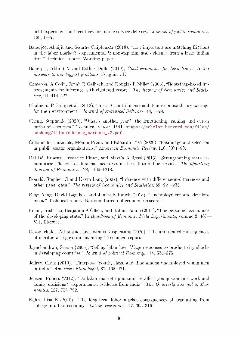
�eld experiment on incentives for public service delivery.� Journal of public economics,120, 1�17.

Banerjee, Abhijit and Gaurav Chiplunkar (2018), �How important are matching frictionsin the labor market? experimental & non-experimental evidence from a large indian�rm.� Technical report, Working paper.

Banerjee, Abhijit V and Esther Du�o (2019), Good economics for hard times: Better

answers to our biggest problems. Penguin UK.

Cameron, A Colin, Jonah B Gelbach, and Douglas L Miller (2008), �Bootstrap-based im-provements for inference with clustered errors.� The Review of Economics and Statis-

tics, 90, 414�427.

Chalmers, R Philip et al. (2012), �mirt: A multidimensional item response theory packagefor the r environment.� Journal of statistical Software, 48, 1�29.

Cheng, Stephanie (2020), �What's another year? the lengthening training and careerpaths of scientists.� Technical report, URL https://scholar.harvard.edu/files/

sdcheng/files/sdcheng_careers_v2.pdf.

Colonnelli, Emanuele, Mounu Prem, and Edoardo Teso (2020), �Patronage and selectionin public sector organizations.� American Economic Review, 110, 3071�99.

Dal Bó, Ernesto, Frederico Finan, and Martín A Rossi (2013), �Strengthening state ca-pabilities: The role of �nancial incentives in the call to public service.� The Quarterly

Journal of Economics, 128, 1169�1218.

Donald, Stephen G and Kevin Lang (2007), �Inference with di�erence-in-di�erences andother panel data.� The review of Economics and Statistics, 89, 221�233.

Feng, Ying, David Lagakos, and James E Rauch (2018), �Unemployment and develop-ment.� Technical report, National bureau of economic research.

Finan, Frederico, Benjamin A Olken, and Rohini Pande (2017), �The personnel economicsof the developing state.� In Handbook of Economic Field Experiments, volume 2, 467�514, Elsevier.

Geromichalos, Athanasios and Ioannis Kospentaris (2020), �The unintended consequencesof meritocratic government hiring.� Technical report.

Jayachandran, Seema (2006), �Selling labor low: Wage responses to productivity shocksin developing countries.� Journal of political Economy, 114, 538�575.

Je�rey, Craig (2010), �Timepass: Youth, class, and time among unemployed young menin india.� American Ethnologist, 37, 465�481.

Jensen, Robert (2012), �Do labor market opportunities a�ect young women's work andfamily decisions? experimental evidence from india.� The Quarterly Journal of Eco-

nomics, 127, 753�792.

Kahn, Lisa B (2010), �The long-term labor market consequences of graduating fromcollege in a bad economy.� Labour economics, 17, 303�316.

40

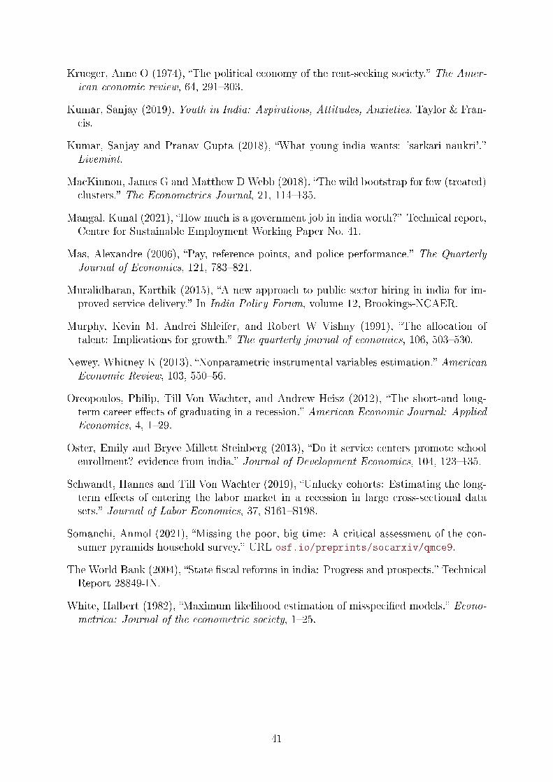
Krueger, Anne O (1974), �The political economy of the rent-seeking society.� The Amer-

ican economic review, 64, 291�303.

Kumar, Sanjay (2019), Youth in India: Aspirations, Attitudes, Anxieties. Taylor & Fran-cis.

Kumar, Sanjay and Pranav Gupta (2018), �What young india wants: 'sarkari naukri'.�Livemint.

MacKinnon, James G and Matthew DWebb (2018), �The wild bootstrap for few (treated)clusters.� The Econometrics Journal, 21, 114�135.

Mangal, Kunal (2021), �How much is a government job in india worth?� Technical report,Centre for Sustainable Employment Working Paper No. 41.

Mas, Alexandre (2006), �Pay, reference points, and police performance.� The Quarterly

Journal of Economics, 121, 783�821.

Muralidharan, Karthik (2015), �A new approach to public sector hiring in india for im-proved service delivery.� In India Policy Forum, volume 12, Brookings-NCAER.

Murphy, Kevin M, Andrei Shleifer, and Robert W Vishny (1991), �The allocation oftalent: Implications for growth.� The quarterly journal of economics, 106, 503�530.

Newey, Whitney K (2013), �Nonparametric instrumental variables estimation.� American

Economic Review, 103, 550�56.

Oreopoulos, Philip, Till Von Wachter, and Andrew Heisz (2012), �The short-and long-term career e�ects of graduating in a recession.� American Economic Journal: Applied

Economics, 4, 1�29.

Oster, Emily and Bryce Millett Steinberg (2013), �Do it service centers promote schoolenrollment? evidence from india.� Journal of Development Economics, 104, 123�135.

Schwandt, Hannes and Till Von Wachter (2019), �Unlucky cohorts: Estimating the long-term e�ects of entering the labor market in a recession in large cross-sectional datasets.� Journal of Labor Economics, 37, S161�S198.

Somanchi, Anmol (2021), �Missing the poor, big time: A critical assessment of the con-sumer pyramids household survey.� URL osf.io/preprints/socarxiv/qmce9.

The World Bank (2004), �State �scal reforms in india: Progress and prospects.� TechnicalReport 28849-IN.

White, Halbert (1982), �Maximum likelihood estimation of misspeci�ed models.� Econo-metrica: Journal of the econometric society, 1�25.

41

42

7 Figures

Figure 1: Recruitment Intensity for Posts Impacted by the Hiring Freeze

(a) Vacancies Noti�ed

(b) Noti�cations Published

Data Source: TNPSC Annual Reports, 1990 to 2010.

Notes: The �gure plots measures of recruitment intensity for posts that were not exemptedby the hiring freeze, i.e. it includes all posts recruited through merit-based exams in the stategovernment except police/�re�ghters, medical sta�, and teachers. The x-axis is the state gov-ernment's �scal year, which runs from April to March of the following calendar year. Red linesmark the beginning and end of the hiring freeze. Fiscal year 2006 is not included in the hiringfreeze since most of this �scal year was not covered by the freeze (the freeze ended in July 2006).

43

Figure 2: What Fraction of Eligible Men Appear for State-level Competitive Exams?

Data Sources: TNPSC Application Data; Census of India, 2001 and 2011.Notes: The application rate is calculated as the total number of unique candidates from TamilNadu who appeared for �group" recruitment exams in the 2013 �scal year divided by an estimateof the eligible population in each education × age group cell from the 2011 Census. Applica-tions across recruitments are considered to be from the same candidate if they have the samename, date of birth, education, gender, and pincode. The group recruitments included in thiscalculation account for 87% of all vacancies and 91% of all applications in the �scal year forcompetitive exams for posts that were not exempted during the hiring freeze. The coarsenessof the x-axis corresponds to the age bins provided by the Census. To account for the two yeargap between TNPSC application data (the earliest year for which such data are available) andCensus data, I multiply the observed count in each education × age group cell by the averagetwo-year growth rate in that cell from the previous decade. That growth rate is calculated as:(population2011/population2001)

1/5.

44

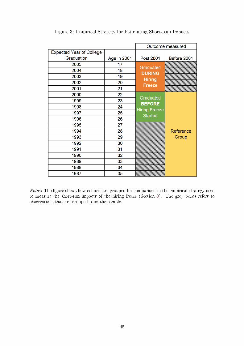
Figure 3: Empirical Strategy for Estimating Short-Run Impacts

Notes: The �gure shows how cohorts are grouped for comparison in the empirical strategy usedto measure the short-run impacts of the hiring freeze (Section 3). The grey boxes refers toobservations that are dropped from the sample.

45

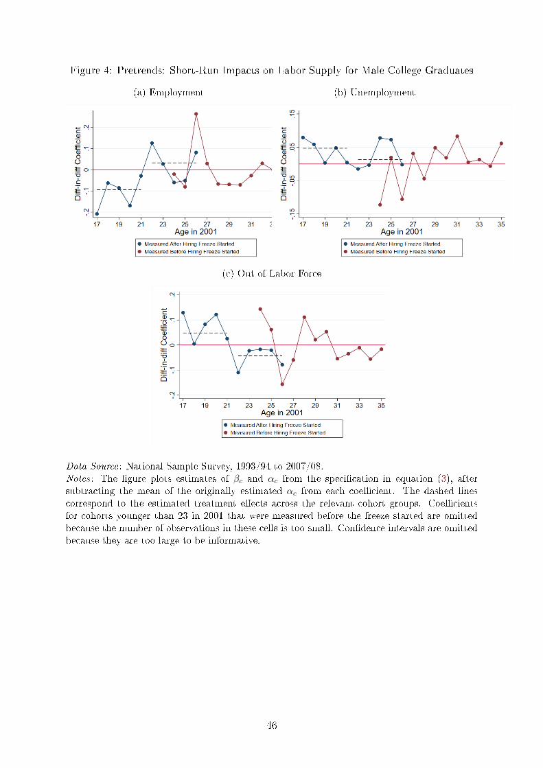
Figure 4: Pretrends: Short-Run Impacts on Labor Supply for Male College Graduates

(a) Employment (b) Unemployment

(c) Out of Labor Force

Data Source: National Sample Survey, 1993/94 to 2007/08.Notes: The �gure plots estimates of βc and αc from the speci�cation in equation (3), aftersubtracting the mean of the originally estimated αc from each coe�cient. The dashed linescorrespond to the estimated treatment e�ects across the relevant cohort groups. Coe�cientsfor cohorts younger than 23 in 2001 that were measured before the freeze started are omittedbecause the number of observations in these cells is too small. Con�dence intervals are omittedbecause they are too large to be informative.

46

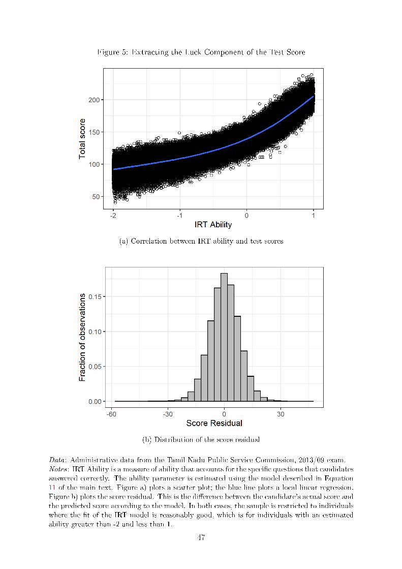
Figure 5: Extracting the Luck Component of the Test Score

(a) Correlation between IRT ability and test scores

(b) Distribution of the score residual

Data: Administrative data from the Tamil Nadu Public Service Commission, 2013/09 exam.Notes: IRT Ability is a measure of ability that accounts for the speci�c questions that candidatesanswered correctly. The ability parameter is estimated using the model described in Equation11 of the main text. Figure a) plots a scatter plot; the blue line plots a local linear regression.Figure b) plots the score residual. This is the di�erence between the candidate's actual score andthe predicted score according to the model. In both cases, the sample is restricted to individualswhere the �t of the IRT model is reasonably good, which is for individuals with an estimatedability greater than -2 and less than 1.

47

Figure 6: Candidates base re-application decisions on past test scores

Data: TNPSC Application and Testing Data, 2012-2016Notes: The �gure plots the impact of score variation in the baseline exam (the 2013 Group 4exam) on subsequent exam-taking. The x-axis plots the years between a particular exam andthe baseline exam (which is the 2013 Group 4 exam). The y-axis plots the estimate of the βcoe�cient from the regression speci�ed in equation (13). This is a regression of a dummy ofwhether the candidate applied for a particular exam and the rank residual on the baseline exam.The error bars plot 95% con�dence intervals.

48

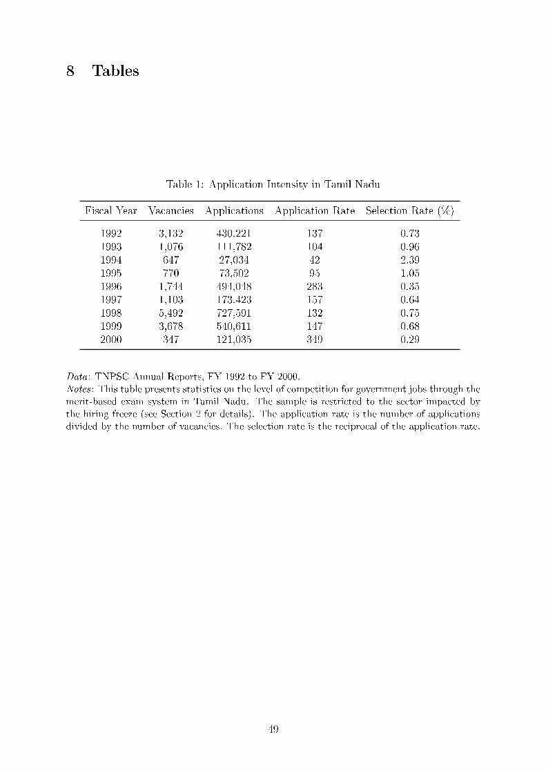
8 Tables

Table 1: Application Intensity in Tamil Nadu

Fiscal Year Vacancies Applications Application Rate Selection Rate (%)

1992 3,132 430,221 137 0.731993 1,076 111,782 104 0.961994 647 27,034 42 2.391995 770 73,502 95 1.051996 1,744 494,048 283 0.351997 1,103 173,423 157 0.641998 5,492 727,591 132 0.751999 3,678 540,611 147 0.682000 347 121,035 349 0.29

Data: TNPSC Annual Reports, FY 1992 to FY 2000.Notes: This table presents statistics on the level of competition for government jobs through themerit-based exam system in Tamil Nadu. The sample is restricted to the sector impacted bythe hiring freeze (see Section 2 for details). The application rate is the number of applicationsdivided by the number of vacancies. The selection rate is the reciprocal of the application rate.

49

Table 2: Short-Run Impacts on Labor Supply for Male College Graduates

(1) (2) (3)Employed Unemployed Out of labor force

Panel A: Di�-in-di� estimates, college sample

TN × Age 17-21 in 2001, Post (β1) -.095∗∗ .047 .048[-.177, -.024] [-.013, .113] [-.015, .113]

TN × Age 22-26 in 2001, Post (β2) .031 .013 -.044[-.055, .118] [-.037, .053] [-.101, .014]

Mean, TN before 2001 .732 .127 .141Observations 47,998 47,998 47,998

Panel B: Di�-in-di� estimates, ineligible sample

TN × Age 17-21 in 2001, Post (β1) -.0004 -.004 .005[-.021, .022] [-.021, .011] [-.01, .026]

TN × Age 22-26 in 2001, Post (β2) .012 -.009∗∗ -.003[-.007, .03] [-.016, -.002] [-.019, .014]

Mean, TN before 2001 .958 .02 .022Observations 208,342 208,342 208,342

Panel C: Triple di�erence estimates

β1 − β1 -.095∗∗ .051∗ .043[-.173, -.02] [-.007, .113] [-.019, .104]

β2 − β2 .019 .022 -.041[-.063, .109] [-.031, .064] [-.094, .018]

Observations 256,340 256,340 256,340

Data: National Sample Survey, 1994 to 2010.Notes: Panel A presents di�erence-in-di�erences estimates of the impact of the hiring freeze onemployment status for the main sample of interest. This sample is: 1) men; 2) who are collegegraduates; 3) who were between the ages of 17 to 35 in 2001. For additional details about thesample construction, see Section 3. Coe�cients correspond to β1 and β2 from equation (1) inthe main text. Panel B presents an over-identi�cation test of the parallel trends assumption,estimating equation (1) on the sample of individuals ineligible for government jobs, i.e. those withless than a 10th standard education. Panel C presents triple di�erence estimates, di�erencingthe coe�cients from Panels A and B. 95% con�dence intervals in brackets, computed via wildbootstrap with 999 replications, clustered by state x cohort level. ∗ p < 0.1, ∗∗ p < 0.05, ∗∗∗

p < 0.01

50

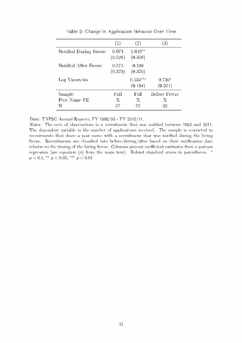
Table 3: Change in Application Behavior Over Time

(1) (2) (3)

Noti�ed During Freeze 0.073 1.049∗∗

(0.526) (0.358)

Noti�ed After Freeze 0.575 0.109(0.379) (0.370)

Log Vacancies 0.534∗∗∗ 0.730∗

(0.104) (0.321)

Sample Full Full Before FreezePost Name FE X X XN 57 57 32

Data: TNPSC Annual Reports, FY 1992/93 - FY 2010/11.Notes: The unit of observations is a recruitment that was noti�ed between 1992 and 2011.The dependent variable is the number of applications received. The sample is restricted torecruitments that share a post name with a recruitment that was noti�ed during the hiringfreeze. Recruitments are classi�ed into before/during/after based on their noti�cation daterelative to the timing of the hiring freeze. Columns present coe�cient estimates from a poissonregression (see equation (4) from the main text). Robust standard errors in parentheses. ∗

p < 0.1, ∗∗ p < 0.05, ∗∗∗ p < 0.01

51

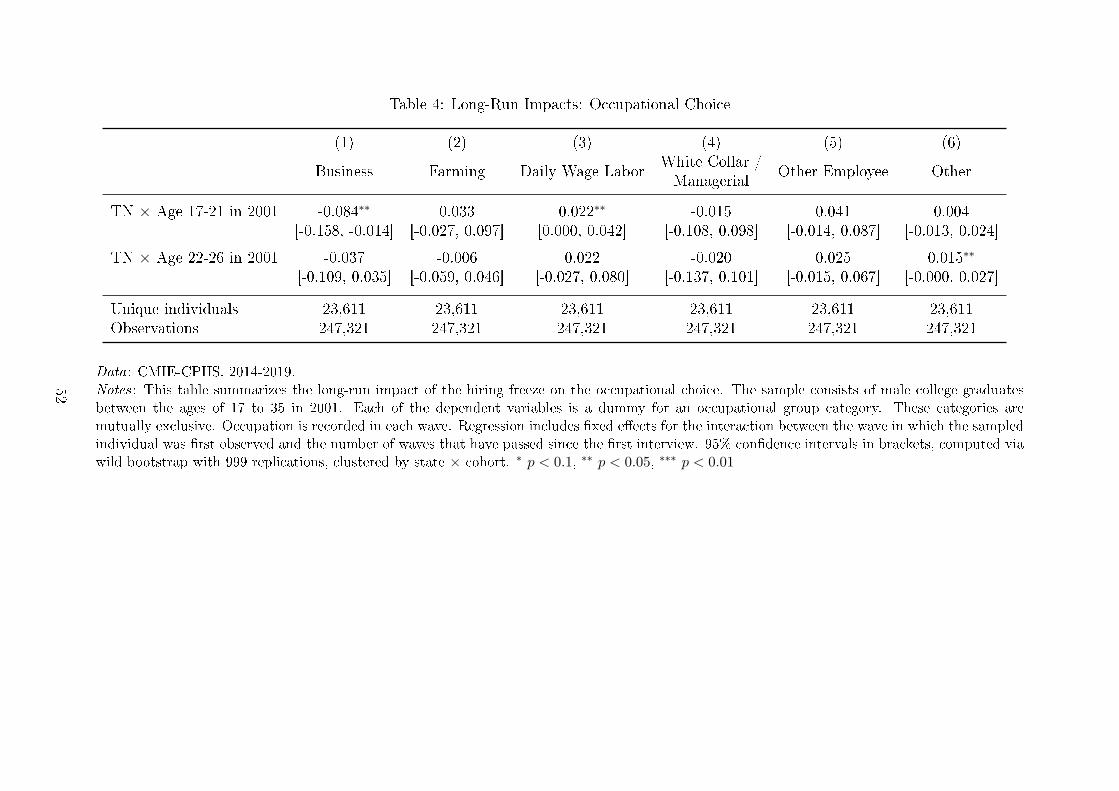
Table 4: Long-Run Impacts: Occupational Choice

(1) (2) (3) (4) (5) (6)

Business Farming Daily Wage LaborWhite Collar /Managerial

Other Employee Other

TN × Age 17-21 in 2001 -0.084∗∗ 0.033 0.022∗∗ -0.015 0.041 0.004[-0.158, -0.014] [-0.027, 0.097] [0.000, 0.042] [-0.108, 0.098] [-0.014, 0.087] [-0.013, 0.024]

TN × Age 22-26 in 2001 -0.037 -0.006 0.022 -0.020 0.025 0.015∗∗

[-0.109, 0.035] [-0.059, 0.046] [-0.027, 0.080] [-0.137, 0.101] [-0.015, 0.067] [-0.000, 0.027]

Unique individuals 23,611 23,611 23,611 23,611 23,611 23,611Observations 247,321 247,321 247,321 247,321 247,321 247,321

Data: CMIE-CPHS, 2014-2019.Notes: This table summarizes the long-run impact of the hiring freeze on the occupational choice. The sample consists of male college graduatesbetween the ages of 17 to 35 in 2001. Each of the dependent variables is a dummy for an occupational group category. These categories aremutually exclusive. Occupation is recorded in each wave. Regression includes �xed e�ects for the interaction between the wave in which the sampledindividual was �rst observed and the number of waves that have passed since the �rst interview. 95% con�dence intervals in brackets, computed viawild bootstrap with 999 replications, clustered by state × cohort. ∗ p < 0.1, ∗∗ p < 0.05, ∗∗∗ p < 0.01

52

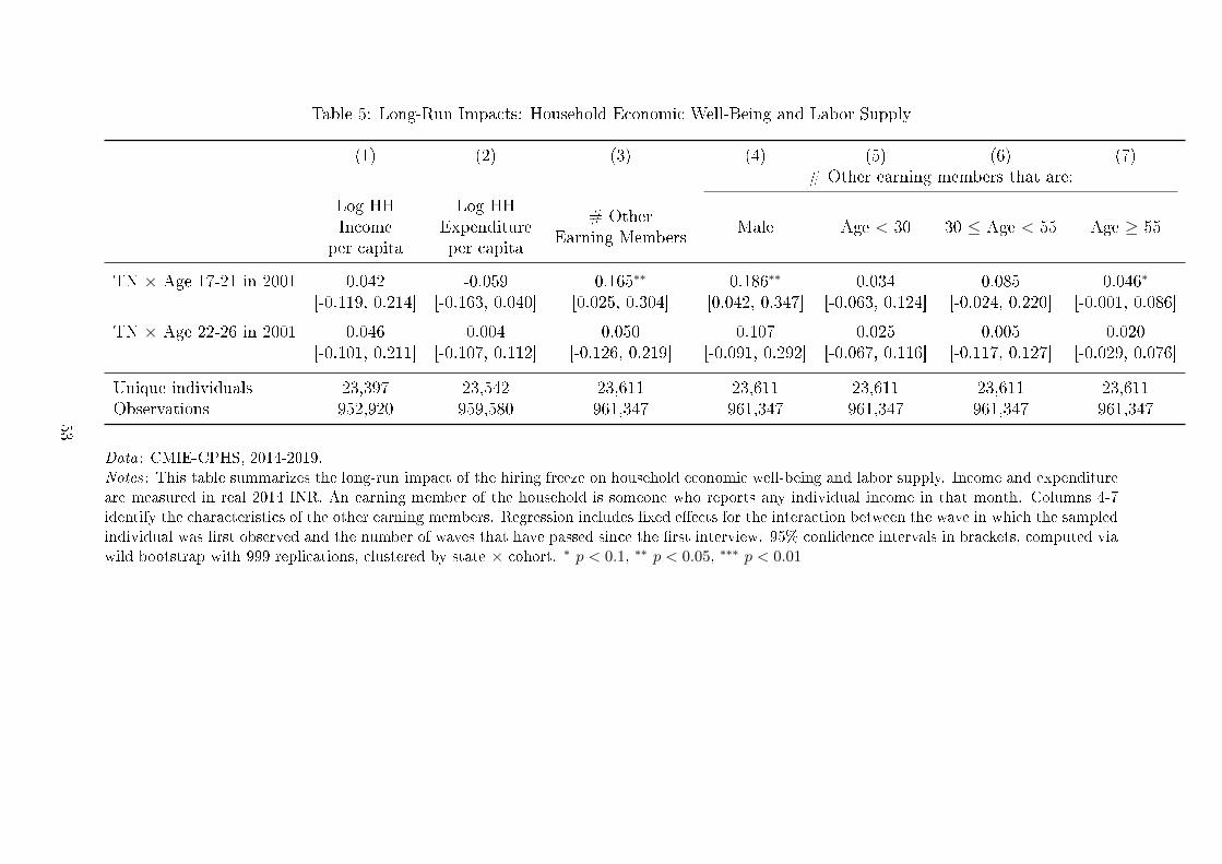
Table 5: Long-Run Impacts: Household Economic Well-Being and Labor Supply

(1) (2) (3) (4) (5) (6) (7)# Other earning members that are:

Log HHIncome

per capita

Log HHExpenditureper capita

# OtherEarning Members

Male Age < 30 30 ≤ Age < 55 Age ≥ 55

TN × Age 17-21 in 2001 0.042 -0.059 0.165∗∗ 0.186∗∗ 0.034 0.085 0.046∗

[-0.119, 0.214] [-0.163, 0.040] [0.025, 0.304] [0.042, 0.347] [-0.063, 0.124] [-0.024, 0.220] [-0.001, 0.086]

TN × Age 22-26 in 2001 0.046 0.004 0.050 0.107 0.025 0.005 0.020[-0.101, 0.211] [-0.107, 0.112] [-0.126, 0.219] [-0.091, 0.292] [-0.067, 0.116] [-0.117, 0.127] [-0.029, 0.076]

Unique individuals 23,397 23,542 23,611 23,611 23,611 23,611 23,611Observations 952,920 959,580 961,347 961,347 961,347 961,347 961,347

Data: CMIE-CPHS, 2014-2019.Notes: This table summarizes the long-run impact of the hiring freeze on household economic well-being and labor supply. Income and expenditureare measured in real 2014 INR. An earning member of the household is someone who reports any individual income in that month. Columns 4-7identify the characteristics of the other earning members. Regression includes �xed e�ects for the interaction between the wave in which the sampledindividual was �rst observed and the number of waves that have passed since the �rst interview. 95% con�dence intervals in brackets, computed viawild bootstrap with 999 replications, clustered by state × cohort. ∗ p < 0.1, ∗∗ p < 0.05, ∗∗∗ p < 0.01

53

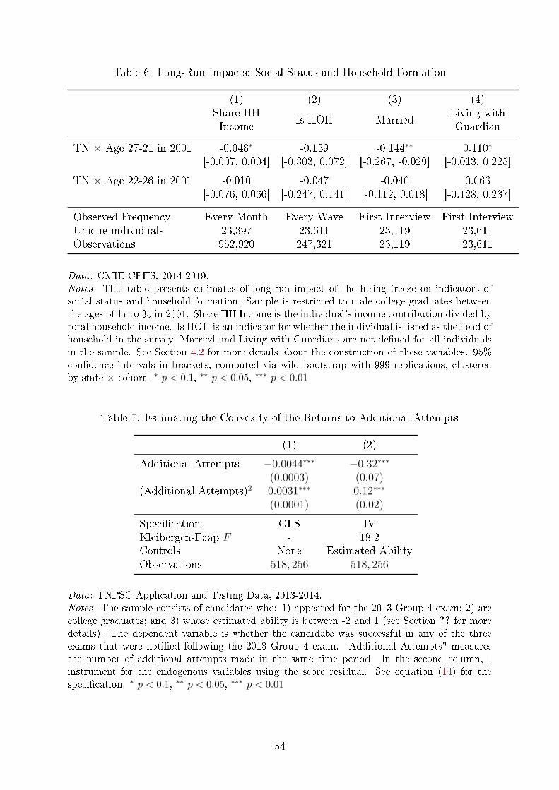
Table 6: Long-Run Impacts: Social Status and Household Formation

(1) (2) (3) (4)Share HHIncome

Is HOH MarriedLiving withGuardian

TN × Age 27-21 in 2001 -0.048∗ -0.139 -0.144∗∗ 0.110∗

[-0.097, 0.004] [-0.303, 0.072] [-0.267, -0.029] [-0.013, 0.225]

TN × Age 22-26 in 2001 -0.010 -0.047 -0.040 0.066[-0.076, 0.066] [-0.247, 0.141] [-0.112, 0.018] [-0.128, 0.237]

Observed Frequency Every Month Every Wave First Interview First InterviewUnique individuals 23,397 23,611 23,119 23,611Observations 952,920 247,321 23,119 23,611

Data: CMIE-CPHS, 2014-2019.Notes: This table presents estimates of long-run impact of the hiring freeze on indicators ofsocial status and household formation. Sample is restricted to male college graduates betweenthe ages of 17 to 35 in 2001. Share HH Income is the individual's income contribution divided bytotal household income. Is HOH is an indicator for whether the individual is listed as the head ofhousehold in the survey. Married and Living with Guardians are not de�ned for all individualsin the sample. See Section 4.2 for more details about the construction of these variables. 95%con�dence intervals in brackets, computed via wild bootstrap with 999 replications, clusteredby state × cohort. ∗ p < 0.1, ∗∗ p < 0.05, ∗∗∗ p < 0.01

Table 7: Estimating the Convexity of the Returns to Additional Attempts

(1) (2)

Additional Attempts −0.0044∗∗∗ −0.32∗∗∗

(0.0003) (0.07)(Additional Attempts)2 0.0031∗∗∗ 0.12∗∗∗

(0.0001) (0.02)

Speci�cation OLS IVKleibergen-Paap F - 18.2Controls None Estimated AbilityObservations 518, 256 518, 256

Data: TNPSC Application and Testing Data, 2013-2014.Notes: The sample consists of candidates who: 1) appeared for the 2013 Group 4 exam; 2) arecollege graduates; and 3) whose estimated ability is between -2 and 1 (see Section ?? for moredetails). The dependent variable is whether the candidate was successful in any of the threeexams that were noti�ed following the 2013 Group 4 exam. �Additional Attempts" measuresthe number of additional attempts made in the same time period. In the second column, Iinstrument for the endogenous variables using the score residual. See equation (14) for thespeci�cation. ∗ p < 0.1, ∗∗ p < 0.05, ∗∗∗ p < 0.01

54

Appendix

Table of Contents

A Additional Figures and Tables 56

B Estimating the Direct Demand E�ect 72

C Measurement Error in Age in the CPHS 75

55

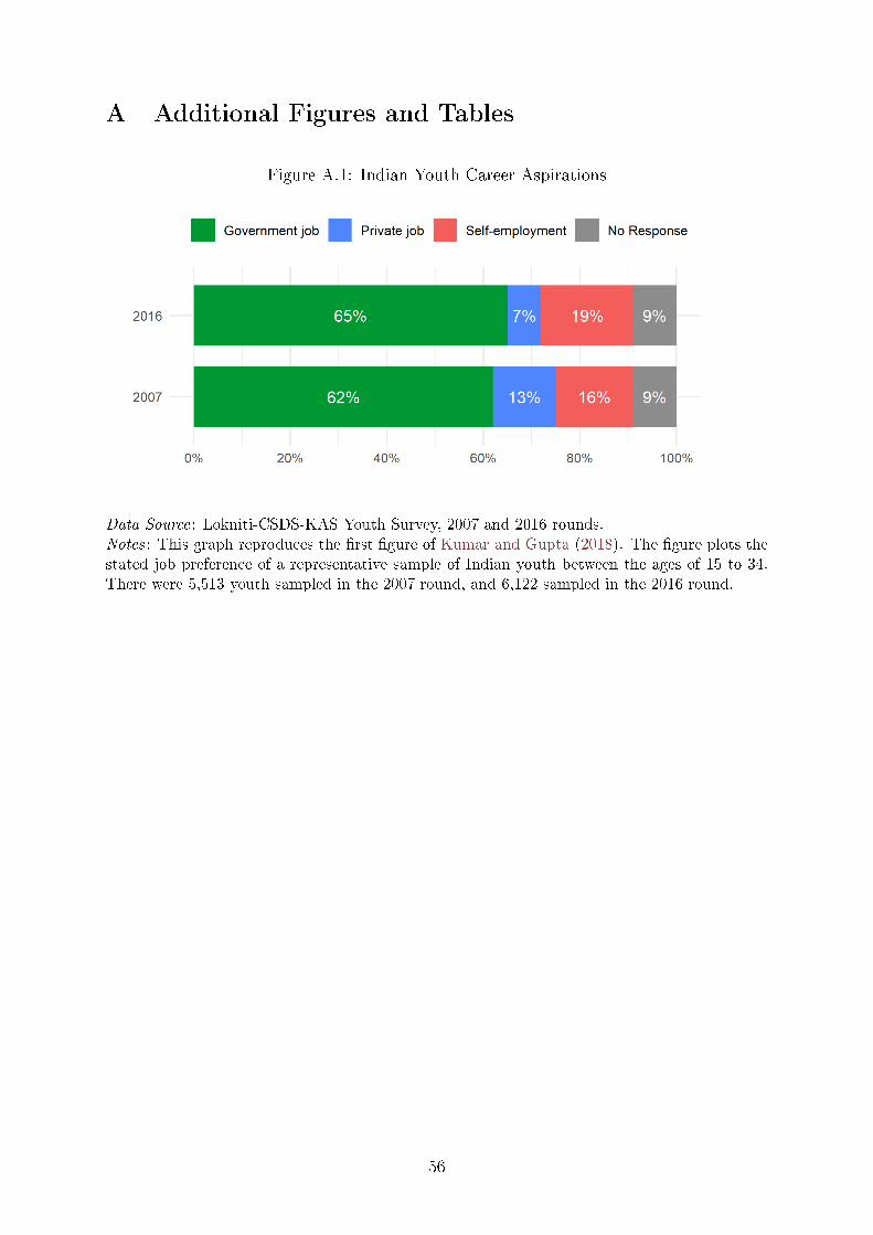
A Additional Figures and Tables

Figure A.1: Indian Youth Career Aspirations

Data Source: Lokniti-CSDS-KAS Youth Survey, 2007 and 2016 rounds.Notes: This graph reproduces the �rst �gure of Kumar and Gupta (2018). The �gure plots thestated job preference of a representative sample of Indian youth between the ages of 15 to 34.There were 5,513 youth sampled in the 2007 round, and 6,122 sampled in the 2016 round.

56

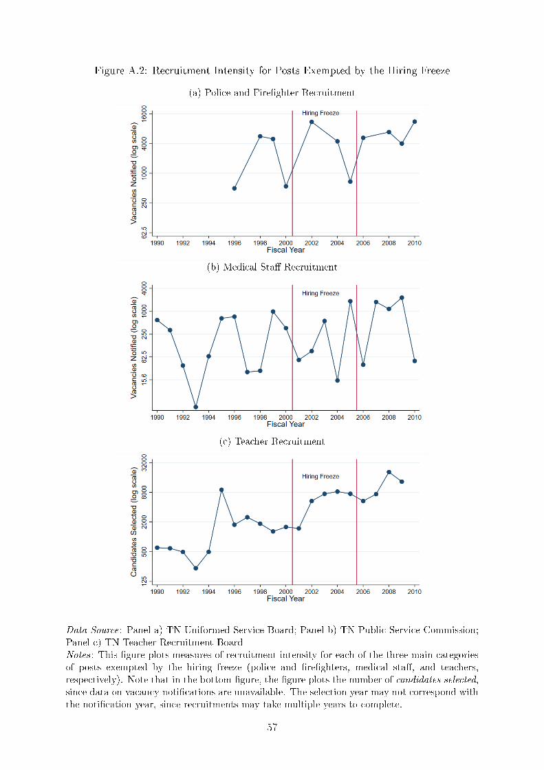
Figure A.2: Recruitment Intensity for Posts Exempted by the Hiring Freeze

(a) Police and Fire�ghter Recruitment

(b) Medical Sta� Recruitment

(c) Teacher Recruitment

Data Source: Panel a) TN Uniformed Service Board; Panel b) TN Public Service Commission;Panel c) TN Teacher Recruitment BoardNotes: This �gure plots measures of recruitment intensity for each of the three main categoriesof posts exempted by the hiring freeze (police and �re�ghters, medical sta�, and teachers,respectively). Note that in the bottom �gure, the �gure plots the number of candidates selected,since data on vacancy noti�cations are unavailable. The selection year may not correspond withthe noti�cation year, since recruitments may take multiple years to complete.

57

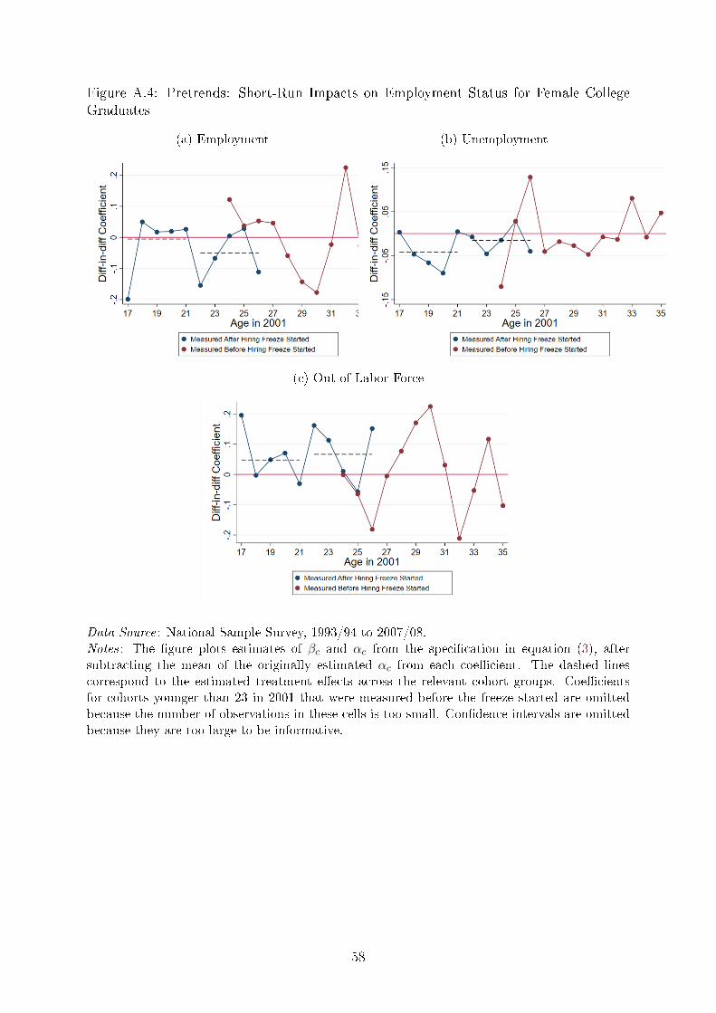
Figure A.4: Pretrends: Short-Run Impacts on Employment Status for Female CollegeGraduates

(a) Employment (b) Unemployment

(c) Out of Labor Force

Data Source: National Sample Survey, 1993/94 to 2007/08.Notes: The �gure plots estimates of βc and αc from the speci�cation in equation (3), aftersubtracting the mean of the originally estimated αc from each coe�cient. The dashed linescorrespond to the estimated treatment e�ects across the relevant cohort groups. Coe�cientsfor cohorts younger than 23 in 2001 that were measured before the freeze started are omittedbecause the number of observations in these cells is too small. Con�dence intervals are omittedbecause they are too large to be informative.

58

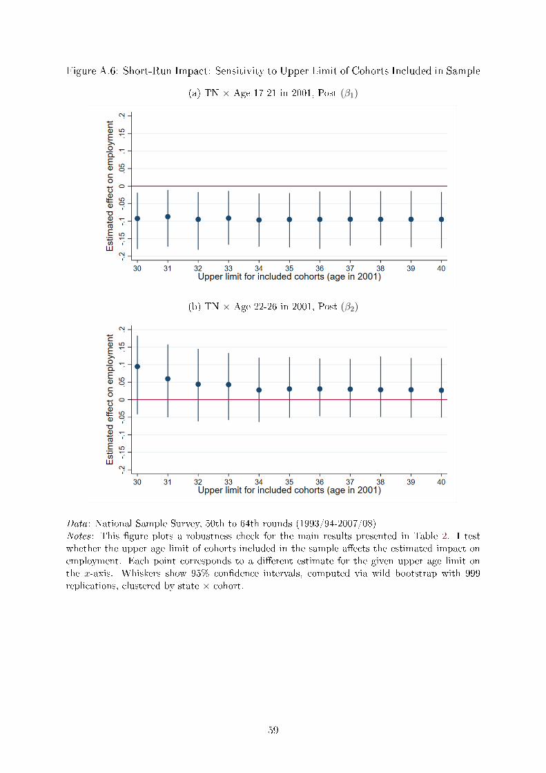
Figure A.6: Short-Run Impact: Sensitivity to Upper Limit of Cohorts Included in Sample

(a) TN × Age 17-21 in 2001, Post (β1)

(b) TN × Age 22-26 in 2001, Post (β2)

Data: National Sample Survey, 50th to 64th rounds (1993/94-2007/08)Notes: This �gure plots a robustness check for the main results presented in Table 2. I testwhether the upper age limit of cohorts included in the sample a�ects the estimated impact onemployment. Each point corresponds to a di�erent estimate for the given upper age limit onthe x-axis. Whiskers show 95% con�dence intervals, computed via wild bootstrap with 999replications, clustered by state × cohort.

59

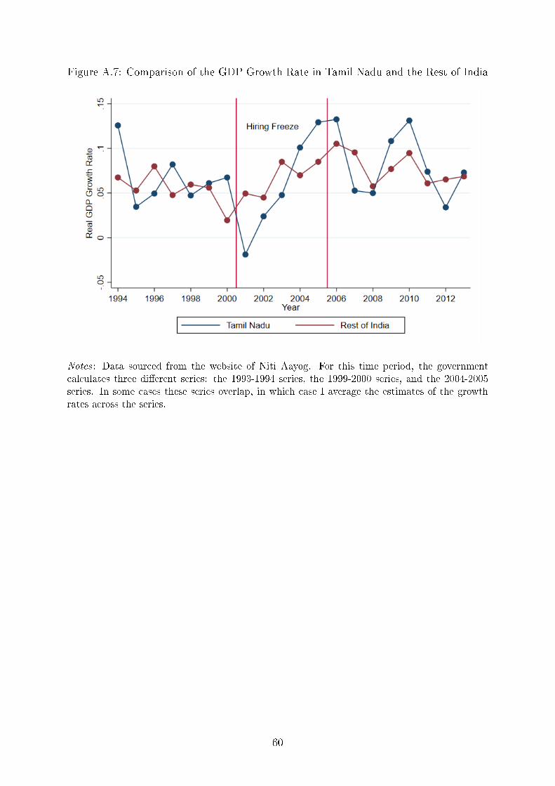
Figure A.7: Comparison of the GDP Growth Rate in Tamil Nadu and the Rest of India

Notes: Data sourced from the website of Niti Aayog. For this time period, the governmentcalculates three di�erent series: the 1993-1994 series, the 1999-2000 series, and the 2004-2005series. In some cases these series overlap, in which case I average the estimates of the growthrates across the series.

60

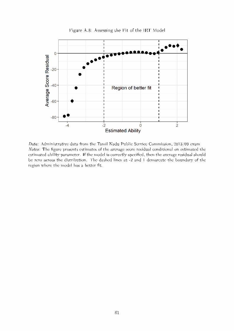
Figure A.8: Assessing the Fit of the IRT Model

Data: Administrative data from the Tamil Nadu Public Service Commission, 2013/09 examNotes: The �gure presents estimates of the average score residual conditional on estimated theestimated ability parameter. If the model is correctly speci�ed, then the average residual shouldbe zero across the distribution. The dashed lines at -2 and 1 demarcate the boundary of theregion where the model has a better �t.

61

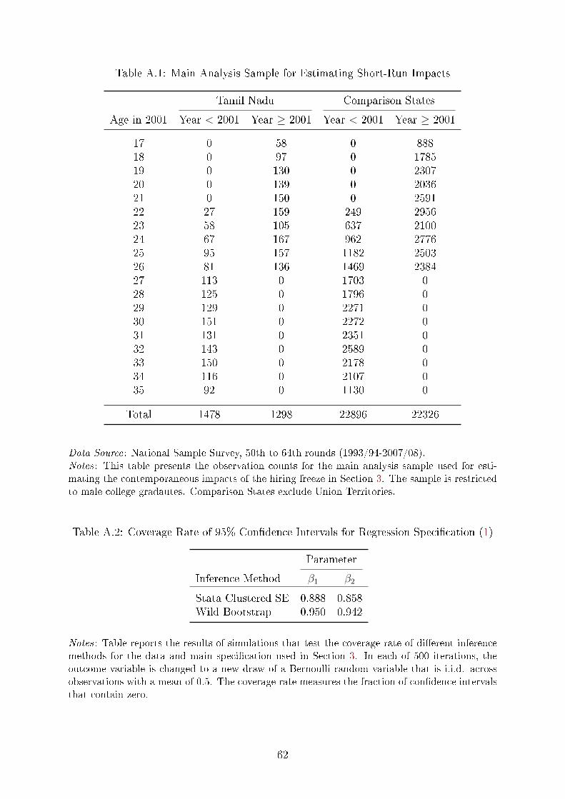
Table A.1: Main Analysis Sample for Estimating Short-Run Impacts

Tamil Nadu Comparison States

Age in 2001 Year < 2001 Year ≥ 2001 Year < 2001 Year ≥ 2001

17 0 58 0 88818 0 97 0 178519 0 130 0 230720 0 139 0 203621 0 150 0 259122 27 159 249 295623 58 105 637 210024 67 167 962 277625 95 157 1182 250326 81 136 1469 238427 113 0 1703 028 125 0 1796 029 129 0 2271 030 151 0 2272 031 131 0 2351 032 143 0 2589 033 150 0 2178 034 116 0 2107 035 92 0 1130 0

Total 1478 1298 22896 22326

Data Source: National Sample Survey, 50th to 64th rounds (1993/94-2007/08).Notes: This table presents the observation counts for the main analysis sample used for esti-mating the contemporaneous impacts of the hiring freeze in Section 3. The sample is restrictedto male college gradautes. Comparison States exclude Union Territories.

Table A.2: Coverage Rate of 95% Con�dence Intervals for Regression Speci�cation (1)

Parameter

Inference Method β1 β2

Stata Clustered SE 0.888 0.858Wild Bootstrap 0.950 0.942

Notes: Table reports the results of simulations that test the coverage rate of di�erent inferencemethods for the data and main speci�cation used in Section 3. In each of 500 iterations, theoutcome variable is changed to a new draw of a Bernoulli random variable that is i.i.d. acrossobservations with a mean of 0.5. The coverage rate measures the fraction of con�dence intervalsthat contain zero.

62

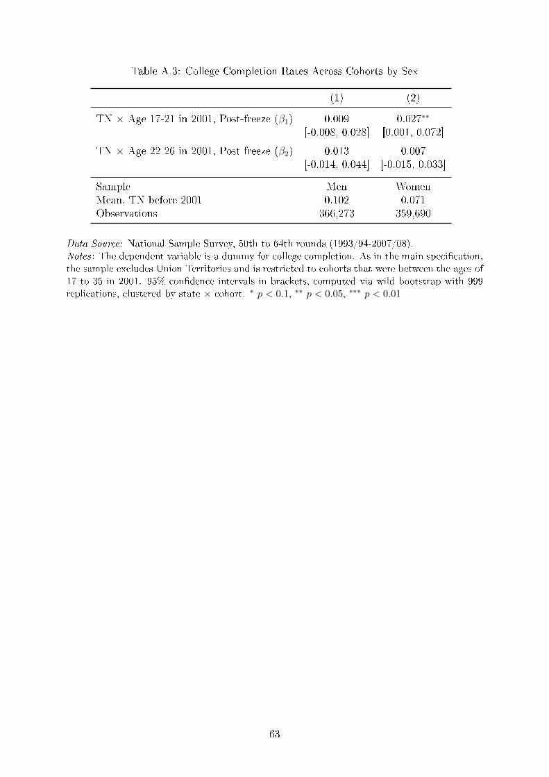
Table A.3: College Completion Rates Across Cohorts by Sex

(1) (2)

TN × Age 17-21 in 2001, Post-freeze (β1) 0.009 0.027∗∗

[-0.008, 0.028] [0.001, 0.072]

TN × Age 22-26 in 2001, Post-freeze (β2) 0.013 0.007[-0.014, 0.044] [-0.015, 0.033]

Sample Men WomenMean, TN before 2001 0.102 0.071Observations 366,273 359,690

Data Source: National Sample Survey, 50th to 64th rounds (1993/94-2007/08).Notes: The dependent variable is a dummy for college completion. As in the main speci�cation,the sample excludes Union Territories and is restricted to cohorts that were between the ages of17 to 35 in 2001. 95% con�dence intervals in brackets, computed via wild bootstrap with 999replications, clustered by state × cohort. ∗ p < 0.1, ∗∗ p < 0.05, ∗∗∗ p < 0.01

63

Table A.4: Short-Run Impacts: Comparison States Restricted to South India

(1) (2) (3)Employed Unemployed Out of labor force

Panel A: Di�-in-di� estimates, college sample

TN × Age 17-21 in 2001, Post (β1) -.071 .053 .018[-.173, .028] [-.018, .127] [-.056, .092]

TN × Age 22-26 in 2001, Post (β2) .063 -.003 -.06[-.055, .172] [-.067, .058] [-.133, .018]

Mean, TN before 2001 .732 .127 .141Observations 9,706 9,706 9,706

Panel B: Di�-in-di� estimates, ineligible sample

TN × Age 17-21 in 2001, Post (β1) .003 -.005 .003[-.025, .034] [-.026, .016] [-.012, .023]

TN × Age 22-26 in 2001, Post (β2) .009 -.008 -.001[-.01, .029] [-.019, .002] [-.017, .017]

Mean, TN before 2001 .958 .02 .022Observations 42,763 42,763 42,763

Panel C: Triple di�erence estimates

β1 − β1 -.074 .058 .015[-.172, .026] [-.015, .132] [-.055, .086]

β2 − β2 .054 .006 -.059[-.062, .173] [-.059, .068] [-.131, .016]

Observations 52,469 52,469 52,469

Notes: 95% con�dence intervals in brackets, computed via wild bootstrap with 999 replications,clustered by state × cohort level. ∗ p < 0.1, ∗∗ p < 0.05, ∗∗∗ p < 0.01

64

Table A.5: Do A�ected Cohorts Remained A�ected in the Medium Term?

(1) (2) (3)Employed Unemployed Out of labor force

Panel A: Di�-in-di� estimates, college sample

TN × Age 17-21 in 2001, Post (β1) .022 -.003 -.019[-.036, .087] [-.041, .041] [-.091, .03]

TN × Age 22-26 in 2001, Post (β2) .007 -.003 -.004[-.075, .161] [-.147, .075] [-.021, .015]

Mean, TN before 2001 .741 .123 .136Observations 36,152 36,152 36,152

Panel B: Di�-in-di� estimates, ineligible sample

TN × Age 17-21 in 2001, Post (β1) .005 -.005 0[-.018, .022] [-.014, .003] [-.015, .019]

TN × Age 22-26 in 2001, Post (β2) 0 -.002 .002[-.028, .028] [-.008, .005] [-.032, .038]

Mean, TN before 2001 .959 .019 .022Observations 153,231 153,231 153,231

Panel C: Triple di�erence estimates

β1 − β1 .017 .003 -.02[-.053, .092] [-.034, .04] [-.104, .038]

β2 − β2 .007 -.001 -.006[-.095, .109] [-.119, .076] [-.043, .035]

Observations 189,383 189,383 189,383

Data Source: National Sample Survey, 50th to 68th rounds (1993/94-2011/12).Notes: 95% con�dence intervals in brackets, computed via wild bootstrap with 999 replications,clustered by state × cohort. ∗ p < 0.1, ∗∗ p < 0.05, ∗∗∗ p < 0.01

65

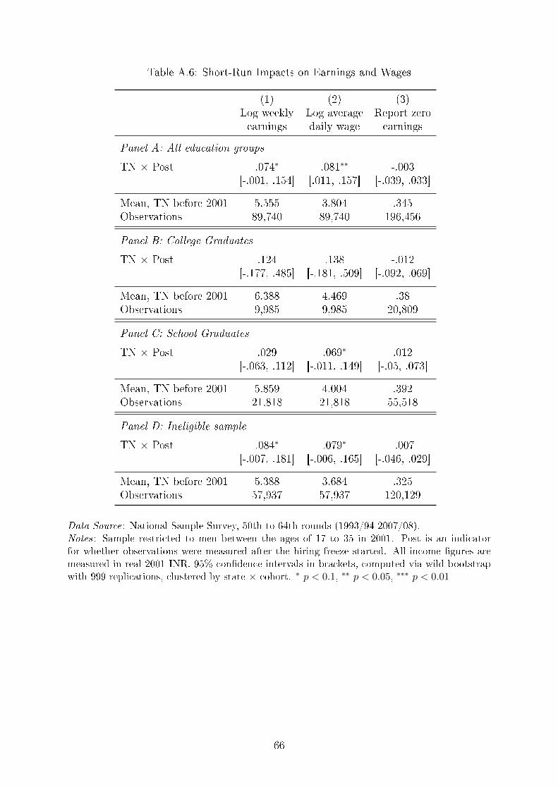
Table A.6: Short-Run Impacts on Earnings and Wages

(1) (2) (3)Log weeklyearnings

Log averagedaily wage

Report zeroearnings

Panel A: All education groups

TN × Post .074∗ .081∗∗ -.003[-.001, .154] [.011, .157] [-.039, .033]

Mean, TN before 2001 5.555 3.804 .345Observations 89,740 89,740 196,456

Panel B: College Graduates

TN × Post .124 .138 -.012[-.177, .485] [-.181, .509] [-.092, .069]

Mean, TN before 2001 6.388 4.469 .38Observations 9,985 9,985 20,809

Panel C: School Graduates

TN × Post .029 .069∗ .012[-.063, .112] [-.011, .149] [-.05, .073]

Mean, TN before 2001 5.859 4.004 .392Observations 21,818 21,818 55,518

Panel D: Ineligible sample

TN × Post .084∗ .079∗ -.007[-.007, .181] [-.006, .165] [-.046, .029]

Mean, TN before 2001 5.388 3.684 .325Observations 57,937 57,937 120,129

Data Source: National Sample Survey, 50th to 64th rounds (1993/94-2007/08).Notes: Sample restricted to men between the ages of 17 to 35 in 2001. Post is an indicatorfor whether observations were measured after the hiring freeze started. All income �gures aremeasured in real 2001 INR. 95% con�dence intervals in brackets, computed via wild bootstrapwith 999 replications, clustered by state × cohort. ∗ p < 0.1, ∗∗ p < 0.05, ∗∗∗ p < 0.01

66

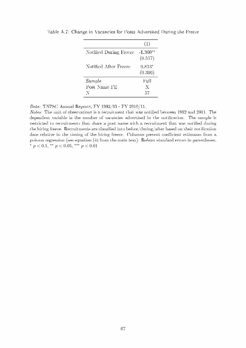
Table A.7: Change in Vacancies for Posts Advertised During the Freeze

(1)

Noti�ed During Freeze -1.360∗∗

(0.517)

Noti�ed After Freeze 0.813∗

(0.396)

Sample FullPost Name FE XN 57

Data: TNPSC Annual Reports, FY 1992/93 - FY 2010/11.Notes: The unit of observations is a recruitment that was noti�ed between 1992 and 2011. Thedependent variable is the number of vacancies advertised in the noti�cation. The sample isrestricted to recruitments that share a post name with a recruitment that was noti�ed duringthe hiring freeze. Recruitments are classi�ed into before/during/after based on their noti�cationdate relative to the timing of the hiring freeze. Columns present coe�cient estimates from apoisson regression (see equation (4) from the main text). Robust standard errors in parentheses.∗ p < 0.1, ∗∗ p < 0.05, ∗∗∗ p < 0.01

67

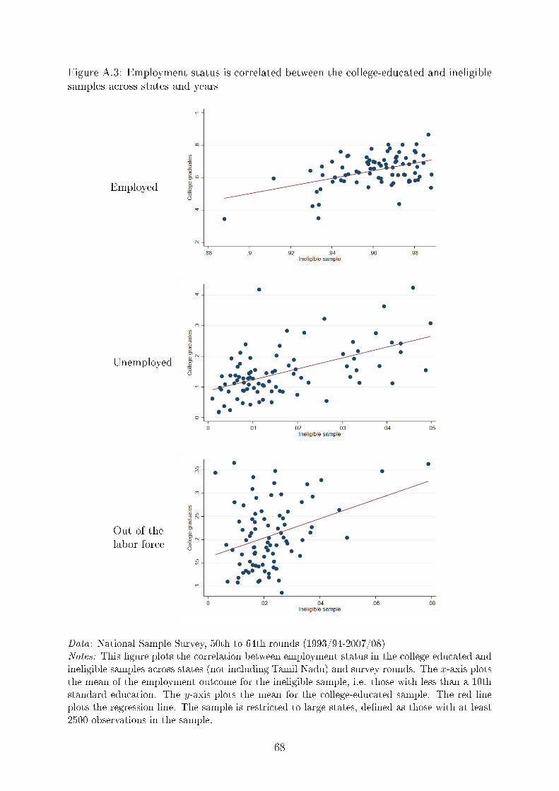
Figure A.3: Employment status is correlated between the college-educated and ineligiblesamples across states and years

Employed

Unemployed

Out of thelabor force

Data: National Sample Survey, 50th to 64th rounds (1993/94-2007/08)Notes: This �gure plots the correlation between employment status in the college educated andineligible samples across states (not including Tamil Nadu) and survey rounds. The x-axis plotsthe mean of the employment outcome for the ineligible sample, i.e. those with less than a 10thstandard education. The y-axis plots the mean for the college-educated sample. The red lineplots the regression line. The sample is restricted to large states, de�ned as those with at least2500 observations in the sample.

68

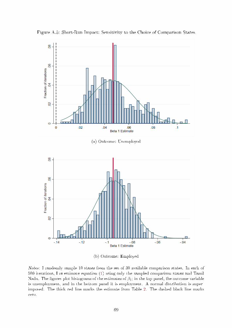
Figure A.5: Short-Run Impact: Sensitivity to the Choice of Comparison States

(a) Outcome: Unemployed

(b) Outcome: Employed

Notes: I randomly sample 10 states from the set of 30 available comparison states. In each of500 iterations, I re-estimate equation (1) using only the sampled comparison states and TamilNadu. The �gures plot histograms of the estimates of β1; in the top panel, the outcome variableis unemployment, and in the bottom panel it is employment. A normal distribution is super-imposed. The thick red line marks the estimate from Table 2. The dashed black line markszero.

69

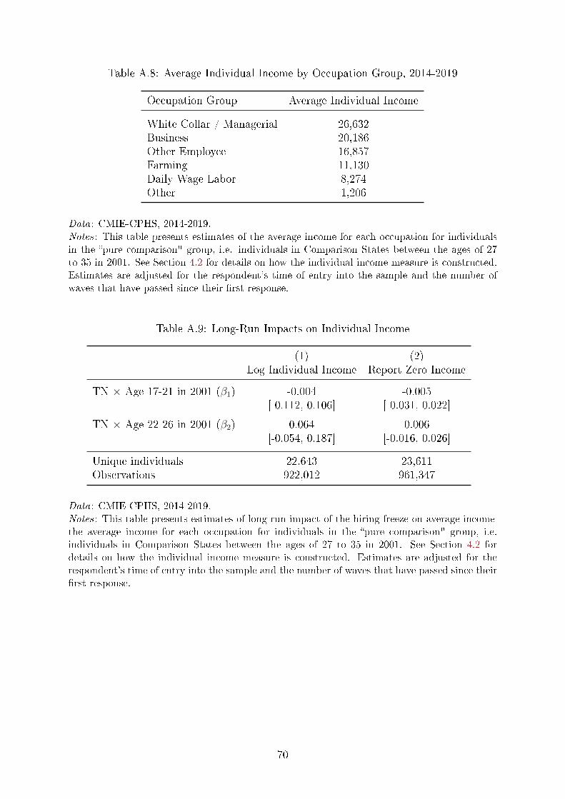
Table A.8: Average Individual Income by Occupation Group, 2014-2019

Occupation Group Average Individual Income

White Collar / Managerial 26,632Business 20,186Other Employee 16,857Farming 11,130Daily Wage Labor 8,274Other 1,206

Data: CMIE-CPHS, 2014-2019.Notes: This table presents estimates of the average income for each occupation for individualsin the �pure comparison" group, i.e. individuals in Comparison States between the ages of 27to 35 in 2001. See Section 4.2 for details on how the individual income measure is constructed.Estimates are adjusted for the respondent's time of entry into the sample and the number ofwaves that have passed since their �rst response.

Table A.9: Long-Run Impacts on Individual Income

(1) (2)Log Individual Income Report Zero Income

TN × Age 17-21 in 2001 (β1) -0.004 -0.005[-0.112, 0.106] [-0.031, 0.022]

TN × Age 22-26 in 2001 (β2) 0.064 0.006[-0.054, 0.187] [-0.016, 0.026]

Unique individuals 22,643 23,611Observations 922,012 961,347

Data: CMIE-CPHS, 2014-2019.Notes: This table presents estimates of long-run impact of the hiring freeze on average incomethe average income for each occupation for individuals in the �pure comparison" group, i.e.individuals in Comparison States between the ages of 27 to 35 in 2001. See Section 4.2 fordetails on how the individual income measure is constructed. Estimates are adjusted for therespondent's time of entry into the sample and the number of waves that have passed since their�rst response.

70

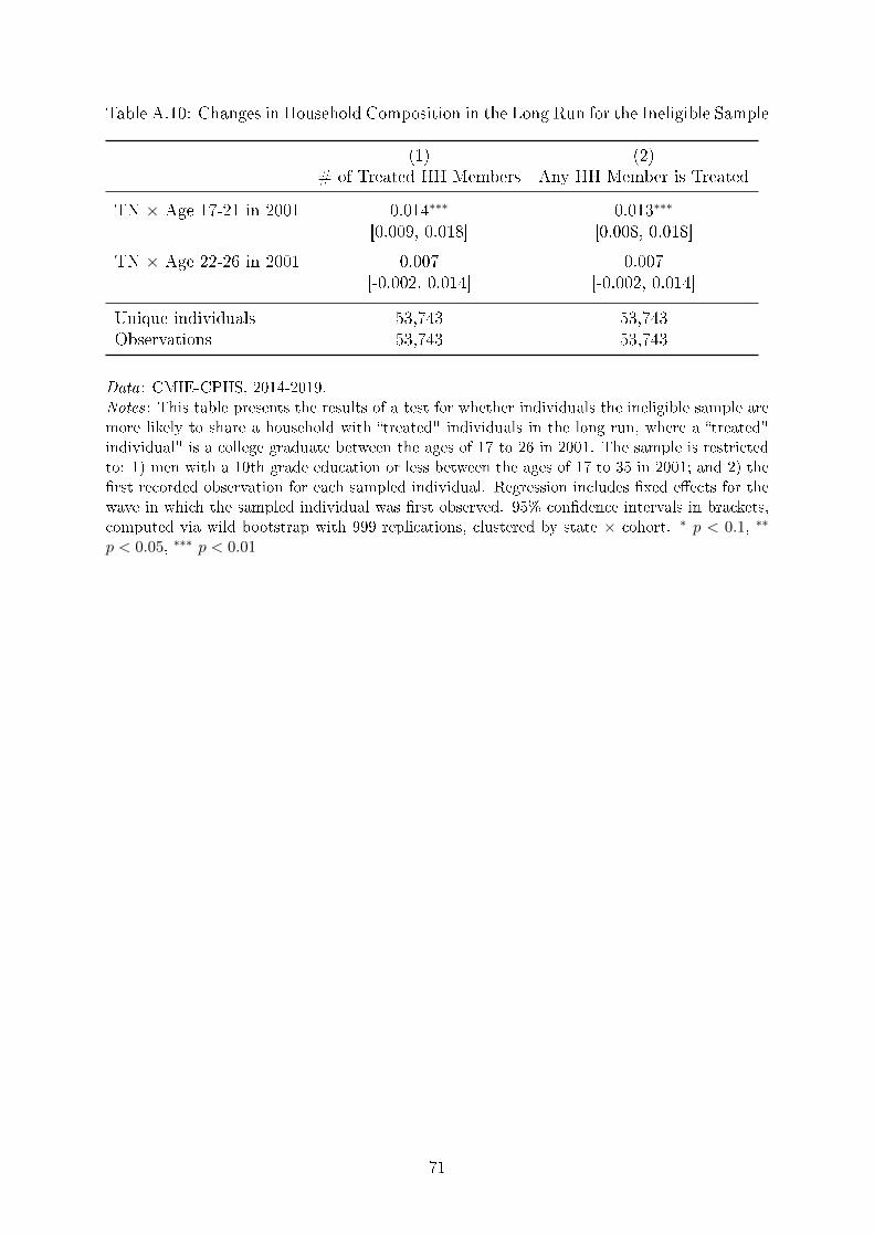
Table A.10: Changes in Household Composition in the Long Run for the Ineligible Sample

(1) (2)# of Treated HH Members Any HH Member is Treated

TN × Age 17-21 in 2001 0.014∗∗∗ 0.013∗∗∗

[0.009, 0.018] [0.008, 0.018]

TN × Age 22-26 in 2001 0.007 0.007[-0.002, 0.014] [-0.002, 0.014]

Unique individuals 53,743 53,743Observations 53,743 53,743

Data: CMIE-CPHS, 2014-2019.Notes: This table presents the results of a test for whether individuals the ineligible sample aremore likely to share a household with �treated" individuals in the long run, where a �treated"individual" is a college graduate between the ages of 17 to 26 in 2001. The sample is restrictedto: 1) men with a 10th grade education or less between the ages of 17 to 35 in 2001; and 2) the�rst recorded observation for each sampled individual. Regression includes �xed e�ects for thewave in which the sampled individual was �rst observed. 95% con�dence intervals in brackets,computed via wild bootstrap with 999 replications, clustered by state × cohort. ∗ p < 0.1, ∗∗

p < 0.05, ∗∗∗ p < 0.01

71

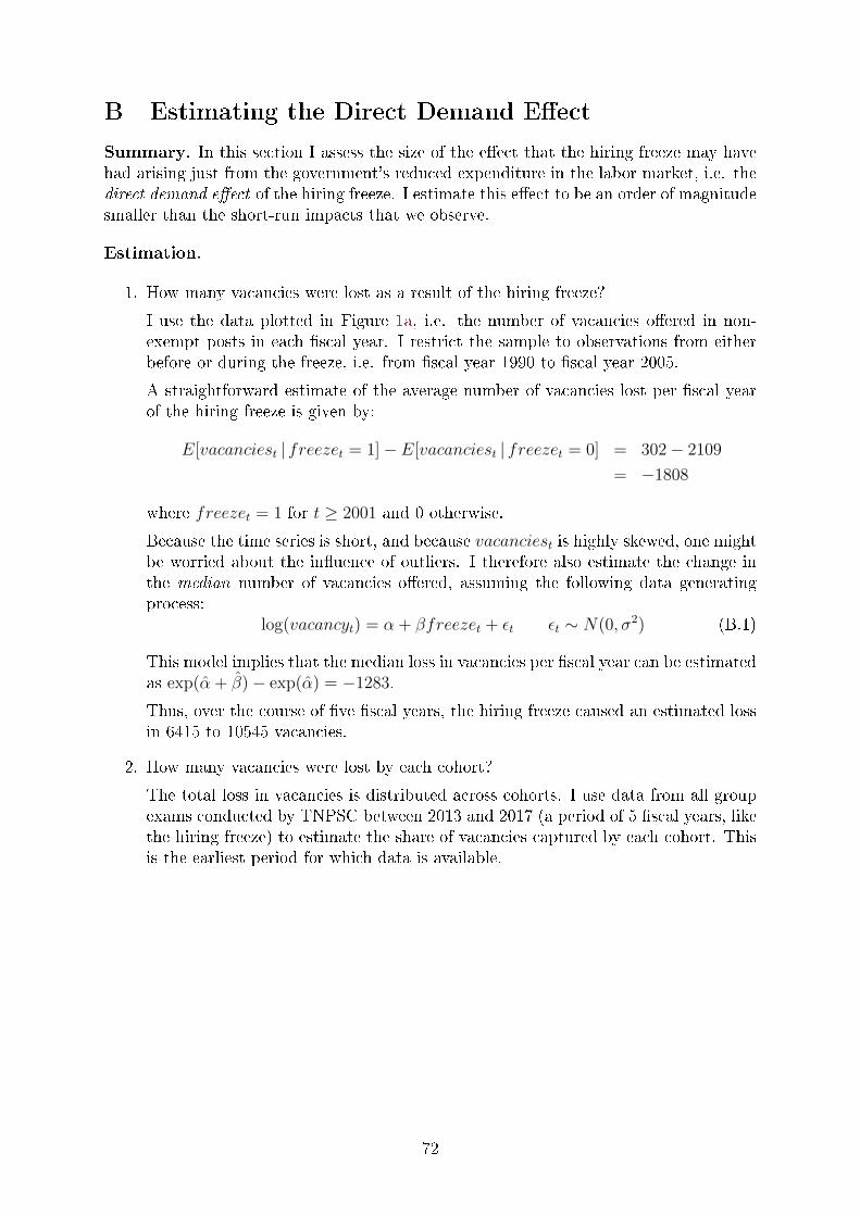
B Estimating the Direct Demand E�ect

Summary. In this section I assess the size of the e�ect that the hiring freeze may havehad arising just from the government's reduced expenditure in the labor market, i.e. thedirect demand e�ect of the hiring freeze. I estimate this e�ect to be an order of magnitudesmaller than the short-run impacts that we observe.

Estimation.

1. How many vacancies were lost as a result of the hiring freeze?

I use the data plotted in Figure 1a, i.e. the number of vacancies o�ered in non-exempt posts in each �scal year. I restrict the sample to observations from eitherbefore or during the freeze, i.e. from �scal year 1990 to �scal year 2005.

A straightforward estimate of the average number of vacancies lost per �scal yearof the hiring freeze is given by:

E[vacanciest | freezet = 1]− E[vacanciest | freezet = 0] = 302− 2109

= −1808

where freezet = 1 for t ≥ 2001 and 0 otherwise.

Because the time series is short, and because vacanciest is highly skewed, one mightbe worried about the in�uence of outliers. I therefore also estimate the change inthe median number of vacancies o�ered, assuming the following data generatingprocess:

log(vacancyt) = α + βfreezet + εt εt ∼ N(0, σ2) (B.1)

This model implies that the median loss in vacancies per �scal year can be estimatedas exp(α + β)− exp(α) = −1283.

Thus, over the course of �ve �scal years, the hiring freeze caused an estimated lossin 6415 to 10545 vacancies.

2. How many vacancies were lost by each cohort?

The total loss in vacancies is distributed across cohorts. I use data from all groupexams conducted by TNPSC between 2013 and 2017 (a period of 5 �scal years, likethe hiring freeze) to estimate the share of vacancies captured by each cohort. Thisis the earliest period for which data is available.

72

Figure B.1: Fraction of vacancies accruing to each cohort, FY 2013 - FY 2017

The results of this calculation are summarized in Figure B.1 above. We see thatmost vacancies are captured by recent college graduates, consistent with their highapplication rates and intense preparation.

Over �ve �scal years, we see that no cohort captures more than 8.75% of the avail-able vacancies. Among male college graduates�the focus of the main analysis�nomore than 5% are captured.

I thus estimate the loss in vacancies to individual cohorts of male college graduatesto be at most:

10545× 0.05 = 527

3. How does the loss in vacancies compare to the size of the labor force in each cohort?

The 2011 Census indicates that were 484,027 male college graduates between theages of 30-34. This is the age category that is closest to the group on which I focusmy analysis (i.e. recent college graduates in 2001 would be ≈ 21). This tells us thatthere were about 484,027 / 5 = 96,805 male college graduates in each individualcohort.

Thus, a loss in 527 vacancies means that about

527/96, 805 = 0.005

or 0.5% of the most a�ected cohorts were delayed in obtaining or did not obtain agovernment job through the competitive exam system.

Note, this is an upper bound, assuming a cohort lost 5 years worth of vacancies.Assuming most college graduates did not plan on applying before they graduated(as Figure 2 suggests) then cohorts who were expected to grduate from collegeduring the hiring freeze would have lost between 1 to 5 years of vacancies, in equalproportion. Thus, the average e�ect across this group is on the order of 0.025%.

73

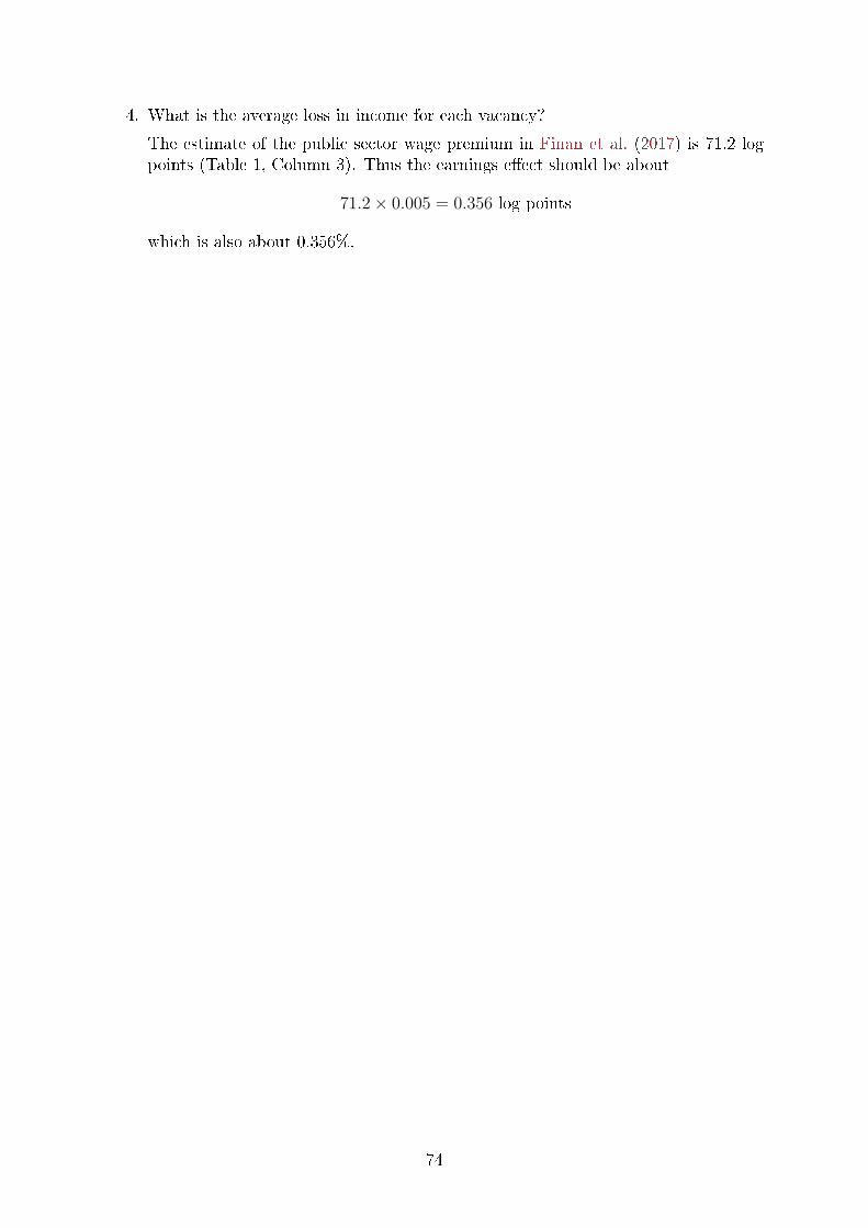
4. What is the average loss in income for each vacancy?

The estimate of the public sector wage premium in Finan et al. (2017) is 71.2 logpoints (Table 1, Column 3). Thus the earnings e�ect should be about

71.2× 0.005 = 0.356 log points

which is also about 0.356%.

74

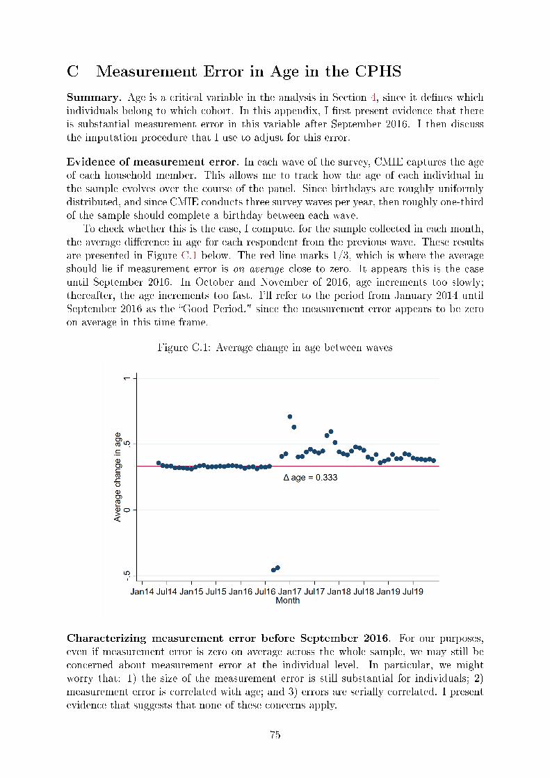
C Measurement Error in Age in the CPHS

Summary. Age is a critical variable in the analysis in Section 4, since it de�nes whichindividuals belong to which cohort. In this appendix, I �rst present evidence that thereis substantial measurement error in this variable after September 2016. I then discussthe imputation procedure that I use to adjust for this error.

Evidence of measurement error. In each wave of the survey, CMIE captures the ageof each household member. This allows me to track how the age of each individual inthe sample evolves over the course of the panel. Since birthdays are roughly uniformlydistributed, and since CMIE conducts three survey waves per year, then roughly one-thirdof the sample should complete a birthday between each wave.

To check whether this is the case, I compute, for the sample collected in each month,the average di�erence in age for each respondent from the previous wave. These resultsare presented in Figure C.1 below. The red line marks 1/3, which is where the averageshould lie if measurement error is on average close to zero. It appears this is the caseuntil September 2016. In October and November of 2016, age increments too slowly;thereafter, the age increments too fast. I'll refer to the period from January 2014 untilSeptember 2016 as the �Good Period," since the measurement error appears to be zeroon average in this time frame.

Figure C.1: Average change in age between waves

Characterizing measurement error before September 2016. For our purposes,even if measurement error is zero on average across the whole sample, we may still beconcerned about measurement error at the individual level. In particular, we mightworry that: 1) the size of the measurement error is still substantial for individuals; 2)measurement error is correlated with age; and 3) errors are serially correlated. I presentevidence that suggests that none of these concerns apply.

75

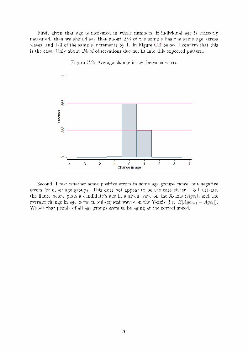
First, given that age is measured in whole numbers, if individual age is correctlymeasured, then we should see that about 2/3 of the sample has the same age acrosswaves, and 1/3 of the sample increments by 1. In Figure C.2 below, I con�rm that thisis the case. Only about 1% of observations due not �t into this expected pattern.

Figure C.2: Average change in age between waves

Second, I test whether some positive errors in some age groups cancel out negativeerrors for other age groups. This does not appear to be the case either. To illustrate,the �gure below plots a candidate's age in a given wave on the X-axis (Aget), and theaverage change in age between subsequent waves on the Y-axis (i.e. E[Aget+1 − Aget]).We see that people of all age groups seem to be aging at the correct speed.

76

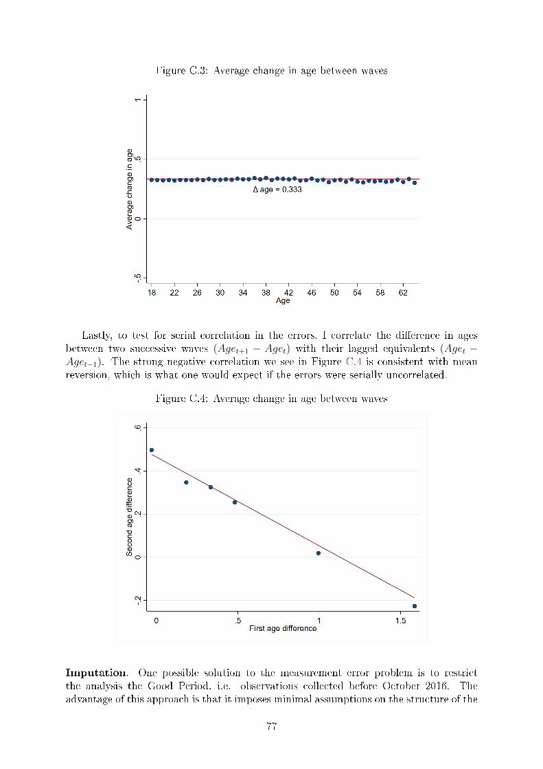
Figure C.3: Average change in age between waves

Lastly, to test for serial correlation in the errors, I correlate the di�erence in agesbetween two successive waves (Aget+1 − Aget) with their lagged equivalents (Aget −Aget−1). The strong negative correlation we see in Figure C.4 is consistent with meanreversion, which is what one would expect if the errors were serially uncorrelated.

Figure C.4: Average change in age between waves

Imputation. One possible solution to the measurement error problem is to restrictthe analysis the Good Period, i.e. observations collected before October 2016. Theadvantage of this approach is that it imposes minimal assumptions on the structure of the

77

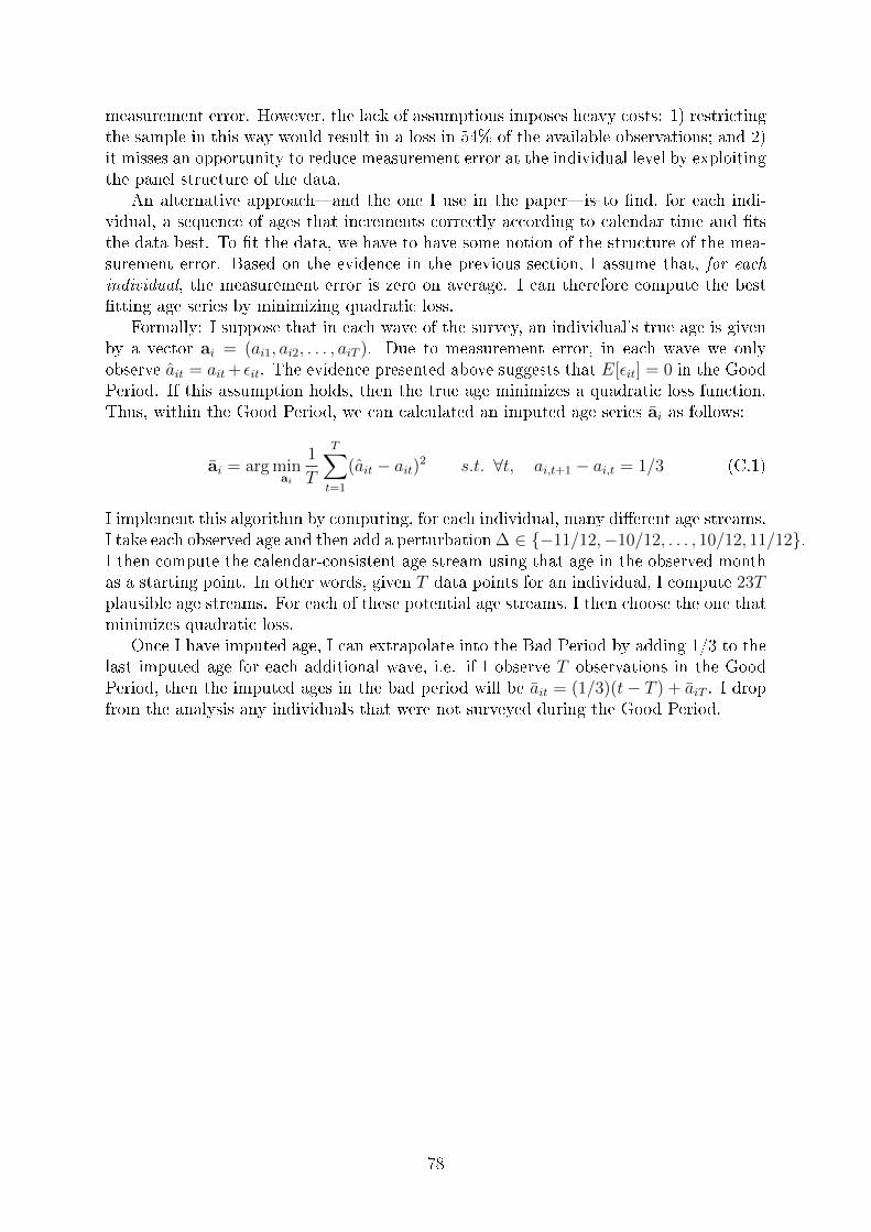
measurement error. However, the lack of assumptions imposes heavy costs: 1) restrictingthe sample in this way would result in a loss in 54% of the available observations; and 2)it misses an opportunity to reduce measurement error at the individual level by exploitingthe panel structure of the data.

An alternative approach�and the one I use in the paper�is to �nd, for each indi-vidual, a sequence of ages that increments correctly according to calendar time and �tsthe data best. To �t the data, we have to have some notion of the structure of the mea-surement error. Based on the evidence in the previous section, I assume that, for each

individual, the measurement error is zero on average. I can therefore compute the best�tting age series by minimizing quadratic loss.

Formally: I suppose that in each wave of the survey, an individual's true age is givenby a vector ai = (ai1, ai2, . . . , aiT ). Due to measurement error, in each wave we onlyobserve ait = ait + εit. The evidence presented above suggests that E[εit] = 0 in the GoodPeriod. If this assumption holds, then the true age minimizes a quadratic loss function.Thus, within the Good Period, we can calculated an imputed age series ai as follows:

ai = arg minai

1

T

T∑t=1

(ait − ait)2 s.t. ∀t, ai,t+1 − ai,t = 1/3 (C.1)

I implement this algorithm by computing, for each individual, many di�erent age streams.I take each observed age and then add a perturbation ∆ ∈ {−11/12,−10/12, . . . , 10/12, 11/12}.I then compute the calendar-consistent age stream using that age in the observed monthas a starting point. In other words, given T data points for an individual, I compute 23Tplausible age streams. For each of these potential age streams, I then choose the one thatminimizes quadratic loss.

Once I have imputed age, I can extrapolate into the Bad Period by adding 1/3 to thelast imputed age for each additional wave, i.e. if I observe T observations in the GoodPeriod, then the imputed ages in the bad period will be ait = (1/3)(t− T ) + aiT . I dropfrom the analysis any individuals that were not surveyed during the Good Period.

78