Competitive Contagion in Networks

Sanjeev Goyal, Hoda Heidari, Michael Kearns

Abstract

We develop a game-theoretic framework for the study of competition between firmswho have budgets to “seed” the initial adoption of their products by consumers locatedin a social network. We identify a general property of the adoption dynamics — namely,decreasing returns to local adoption — for which the inefficiency of resource use atequilibrium (the Price of Anarchy) is uniformly bounded above, across all networks. Wealso show that if this property is violated the Price of Anarchy can be unbounded, thusyielding sharp threshold behavior for a broad class of dynamics.

We provide similar results a new notion, the Budget Multiplier , that measures theextent that imbalances in player budgets can be amplified at equilibrium.

Keywords:

1. Introduction

The role of social networks in shaping individual choices has been brought out in a num-ber of studies over the years.1 In the past, the deliberate use of such social influencesby external agents was hampered by the lack of good data on social networks. In recentyears, data from on-line social networking sites along with other advances in informa-tion technology have created interest in ways that firms and governments can use socialnetworks to further their goals.2

In this work, we study competition between firms who use their resources to maximizeproduct adoption by consumers located in a social network. 3 The social network maytransmit information about products, and adoption of products by neighbors may havedirect consumption benefits. The firms, denoted Red and Blue, know the graph whichdefines the social network and offer similar or interchangeable products or services. Thetwo firms simultaneously choose to allocate their resources on subsets of consumers, i.e.,

Email addresses: sg472@cam.ac.uk (Sanjeev Goyal), hoda@seas.upenn.edu (Hoda Heidari),mkearns@cis.upenn.edu (Michael Kearns)

1See e.g., Coleman [1] on doctors’ prescription of new drugs, Conley and Udry [2] and Foster andRosenzweig [3] on farmers’ decisions on crop and input choice, and Feick and Price [4], Reingen et al. [5],and Godes and Mayzlin [6] on brand choice by consumers.

2The popularity of terms such as word of mouth marketing, viral marketing, seeding the network andpeer-leading intervention is an indicator of this interest.

3Our model may apply to other settings of competitive contagion, such as between two fatal virusesin a population.

Preprint submitted to Games and Economic Behavior March 10, 2014

to seed the network with initial adoptions. The stochastic dynamics of local adoptiondetermine how the influence of each player’s seeds spreads throughout the graph to createnew adoptions. Our work thus builds upon recent interest in models of competitivecontagion [7, 8, 9].

A distinctive feature of our framework is that we allow for a broad class of localinfluence processes. We decompose the dynamics into two parts: a switching function f ,which specifies the probability of a consumer switching from non-adoption to adoption asa function of the fraction of his neighbors who have adopted either of the two productsRed and Blue; and a selection function g, which specifies, conditional on switching, theprobability that the consumer adopts (say) Red as function of the fraction of adoptingneighbors who have adopted Red (the decomposition into switching and selection hassome precursors in the literature, see [8] for example). Each firm seeks to maximizethe total number of consumers who adopt its product. Broadly speaking, the switchingfunction captures “stickiness” of the (interchangeable) products based on their localprevalence, and the selection function captures preference for firms based on local marketshare.

This framework yields a rich class of competitive strategies, which depend in subtleways on the dynamics, the relative budgets of the players, and the structure of the socialnetwork. Section 5 illustrates this point: We will see that even in a simple fixed network,the equilibrium solution depends greatly on the parameters of the model. Also we willsee how these parameters affect other properties of the equilibrium, such as the Price ofAnarchy and the Budget Multiplier.

We then continue with understanding two general features of equilibrium: first, theefficiency of resource use by the players (Price of Anarchy, and Price of Stability) andsecond, the role of the network and dynamics in amplifying ex-ante resource differencesbetween the players (Budget Multiplier).

Our first set of results concern efficiency of resource use by the players. For a fixedgraph and fixed local dynamics (given by f and g), and budgets of KR and KB seedinfections for the players, let (SR, SB) be the sets of seed infections that maximize thejoint expected infections (payoffs) ΠR(SR, SB) + ΠB(SR, SB) subject to |SR| = KR and|SB | = KB , and let σ′R and σ′B be Nash equilibrium strategies obeying the budgetconstraints that minimize the joint payoff ΠR(σR, σB) + ΠB(σR, σB) across all Nashequilibria (σR, σB). The Price of Anarchy (or PoA)4 is then defined as:

ΠR(SR, SB) + ΠB(SR, SB)

ΠR(σ′R, σ′B) + ΠB(σ′R, σ

′B).

Similarly, if σ′′R and σ′′B are Nash equilibrium strategies obeying the budget constraintsthat maximize the joint payoff ΠR(σR, σB) + ΠB(σR, σB) across all Nash equilibria(σR, σB), the Price of Stability (or PoS)5 is then defined as:

ΠR(SR, SB) + ΠB(SR, SB)

ΠR(σ′′R, σ′′B) + ΠB(σ′′R, σ

′′B).

4The PoA is a measure of the maximum potential inefficiency created by non-cooperative/decentralized activity. In our context, if we suppose that consumers get positiveutility from consumption of firms’ products then the PoA also reflects losses in consumer welfare.

5The Price of Stability (PoS) compares outcomes in the ‘best’ equilibrium with socially optimal out-comes; one may interpret the PoS as a measure of the minimum inefficiency created by non-cooperative,as opposed to merely decentralized, activity.

2

Our first main result, Theorem 1, shows that if the switching function f is concaveand the selection function g is linear, then the PoA (and as a result, the PoS) is uni-formly bounded above by 4, across all networks. The main proof technique we employis the construction of certain coupled stochastic dynamical processes that allow us todemonstrate that, under the assumptions on f and g, the departure of one player canonly benefit the other player, even though the total number of joint infections can onlydecrease. This in turn lets us argue that players can successfully defect to the maximumsocial welfare solution and realize a significant fraction of its payoff, thus implying theymust also do so at equilibrium.

Our next main result, Theorem 2, shows that even a small amount of convexity inthe switching function f can lead to arbitrarily high PoS (and as a result PoA). Thisresult is obtained by constructing a family of layered networks whose dynamics effectivelycompose f many times, thus amplifying its convexity. Equilibrium and large PoS areenforced by the fact that despite this amplification, the players are better off playingnear each other: this means that if one player locates in one part of the network, theother player has an incentive to locate close by, even if they would jointly be better offlocating in a different part of the network. Taken together, our upper and lower boundsyield sharp threshold behavior in a parametric classes of dynamics. For example, if theswitching function is f(x) = xr for r > 0 and the selection function g is linear, then forall r ≤ 1 the PoA is at most 4, while for any r > 1 it can be unbounded.

Our second set of results are about the effects of networks and dynamics on budgetdifferences across the players. We introduce and study a new quantity called the BudgetMultiplier . For any fixed graph, local dynamics, and initial budgets, with KR ≥ KB , let(σR, σB) be the Nash equilibrium for which the quantity

ΠR(σR, σB)

ΠB(σR, σB)× KB

KR

is maximized ; this quantity is just the ratio of the final payoffs divided by the ratio ofthe initial budgets. The resulting maximized quantity is the Budget Multiplier, and itmeasures the extent to which the larger budget player can obtain a final market sharethat exceeds their share of the initial budgets.

Theorem 3 shows that if the switching function is concave and the selection functionis linear, then the (pure strategy) Budget Multiplier is bounded above by 2, uniformlyacross all networks. The proof imports elements of the proof for the PoA upper bound,and additionally employs a method for attributing adoptions back to the initial seedsthat generated them.

Our next result, Theorem 4, shows that even a slight departure from linearity inthe selection function can yield unbounded Budget Multiplier. The proof again appealsto network structures that amplify the nonlinearity of g by self-composition, which hasthe effect of “squeezing out” the player with smaller budget. Combining the BudgetMultiplier upper and lower bounds again allows us to exhibit simple parametric formsyielding threshold behavior: for instance, if f is linear and g is from the well-studiedTullock contest function family (discussed shortly), which includes linear g and thereforebounded Budget Multiplier, even an infinitesimal departure from linearity can result inunbounded Budget Multiplier.

3

2. Related Literature

Our paper contributes to the study of competitive strategy in network environments.We build a framework which combines ideas from economics (contests, competitive seed-ing and advertising) and computer science – uniform bounds on properties of equilibria, asin the Price of Anarchy – to address a topical and natural question. The Tullock contestfunction was introduced in Tullock [10]; for an axiomatic development see Skaperdas [11].For early and influential studies of competitive advertising, see Butters [12] and Gross-man and Shapiro [13] . The Price of Anarchy (PoA) was introduced by Koutsoupias andPapadimitriou [14], and important early results bounding the PoA in networked settingsregardless of network structure were given by Roughgarden and Tardos [15]. The tensionbetween equilibrium and Nash efficiency is a recurring theme in economics; for a generalresult on the inefficiency of Nash equilibria, see Dubey [16].

More specifically, we contribute to the study of influence in networks. This hasbeen an active field of study in the last decade, see e.g., Ballester, Calvo-Armengol andZenou [17]; Bharathi, Kempe and Salek [7]; Galeotti and Goyal [18]; Kempe, Kleinberg,and Tardos [19, 20]; Mossel and Roch [21]; Borodin, Filmus, and Oren [8]; Chasparisand Shamma [9]; Carnes et al [22]; Dubey, Garg and De Meyer [23]; Vetta [24]. Thereare three elements in our framework which appear to be novel: one, we consider a fairlygeneral class of adoption rules at the individual consumer level which correspond todifferent roles which social interaction can potentially play (existing work often considersspecific local dynamics); two, we study competition for influence in a network (existingwork has often focused on the case of a single player seeking to maximize influence),and three, we introduce and study the notion of Budget Multiplier as a measure of hownetworks amplify budget differences. To the best of our knowledge, our results on therelationship between the dynamics and qualitative features of the strategic equilibriumare novel. Nevertheless, there are definite points of contact between our results and prooftechniques and earlier research in (single-player and competitive) contagion in networksthat we shall elaborate on where appropriate.

3. Model

3.1. Graph, Allocations, and Seeds

We consider a 2-player game of competitive adoption on a (possibly directed) graphG over n vertices. G is known to the two players, whom we shall refer to as R(ed) andB(lue). 6 We shall also use R,B and U(ninfected) to denote the state of a vertex inG, according to whether it is currently infected by one of the two players or uninfected(Note that we are overloading the notation by giving the same name to the nodes’ statesand to the players, however throughout it will be clear from the context which one weare referring to). The two players simultaneously choose some number of vertices toinitially seed; after this seeding, the stochastic dynamics of local adoption (discussedbelow) determine how each player’s seeds spread throughout G to create adoptions by

6The restriction to 2 players is primarily for simplicity; our main results on PoA can be generalizedto a game with 2 or more players, see Appendix B.

4

new nodes. Each player seeks to maximize their (expected) total number of eventualadoptions. 7

More precisely, suppose that player p = R,B has budget Kp ∈ N+; Each playerp chooses an allocation of budget across the n vertices, ap = (ap1, ap2, ..., apn), whereapj ∈ N+ and

∑nj=1 apj = Kp. Let Lp be the set of allocations for player p, which is

their pure strategy space. A mixed strategy for player p is a probability distribution σpon Lp. Let Ap denote the set of probability distributions for player p. The two playerssimultaneously choose their strategies (σR, σB). Consider any realized initial allocation(aR, aB) for the two players. Let V (aR) = {v|avR > 0}, V (aB) = {v|avB > 0} andlet V (aR, aB) = V (aR) ∪ V (aB). A vertex v becomes initially infected if one or moreplayers assigns a seed to infect v. If both players assign seeds to the same vertex, thenthe probability of initial infection by a player is proportional to the seeds allocated bythe player (relative to the other player). More precisely, fix any allocation (aR, aB). Forany vertex v, the initial state sv of v is in {R,B} if and only if v ∈ V (aR, aB). Moreover,sv = R with probability avR/(avR+avB), and sv = B with probability avB/(avR+avB).

Following the allocation of seeds, the stochastic contagion process on G determineshow these R and B infections generate new adoptions in the network. We considera discrete time model for this process. The state of a vertex v at time t is denotedsvt ∈ {U,R,B}, where U stands for Uninfected, R stands for infection by R, and Bstands for infection by B.

3.2. The Switching-Selection Model

We assume there is an update schedule which determines the order in which verticesare considered for state updates. The primary simplifying assumption we shall makeabout this schedule is that once a vertex is infected, it is never a candidate for updatingagain.

Within this constraint, we allow for a variety of behaviors, such as randomly choosingan uninfected vertex to update at each time step (a form of sequential updating), orupdating all uninfected vertices simultaneously at each time step (a form of parallelupdating). We can also allow for an immunity property — if a vertex is exposed onceto infection and remains uninfected after updating, it is never updated again. Updateschedules may also have finite termination times or conditions — for instance, if thefirms primarily care about the number of adoptions in the coming fiscal year. We canalso allow schedules that update each uninfected vertex only a fixed number of times. Inour framework, a schedule which perpetually updates uninfected vertices will eventuallycause any connected G to become entirely infected, thus trivializing the PoA (though notnecessarily the Budget Multiplier), but we allow for considerably more general schedules.8

For the stochastic update of an uninfected vertex v, we will consider what we shall callthe switching-selection model. In this model, updating is determined by the applicationof two functions to v’s local neighborhood: f(x) (the switching function), and g(y) (theselection function). More precisely, let αR and αB be the fraction of v’s neighbors

7Throughout the paper, we shall use the terms infection and adoption interchangeably.8The proof of Lemma 1 specifies the technical property we need of the update schedule, which is

consistent with the examples mentioned here and many others.

5

infected by R and B, respectively, at the time of the update, and let α = αR + αB bethe total fraction of infected neighbors. The function f maps α to the interval [0, 1] andg maps αR/(αR +αB) (the relative fraction of infections that are R) to [0, 1]. These twofunctions determine the stochastic update in the following fashion:

1. With probability f(α), v becomes infected by either R or B; with probability1− f(α), v remains in state U(ninfected), and the update ends.

2. If it is determined that v becomes infected, it becomes infected by R with proba-bility

g(αR/(αR + αB)),

and infected by B with probability

g(αB/(αR + αB)).

We assume f(0) = 0 (infection requires exposure), f(1) = 1 (full neighborhood infectionforces infection), and f is increasing (more exposure yields more infection); and g(0) = 0(players need some local market share to win an infection), g(1) = 1. Note that since theselection step above requires that an infection take place, we also have g(y)+g(1−y) = 1,which implies g(1/2) = 1/2. We assume that the switching and selection functions arethe same across vertices.9

We think of the switching function as specifying how rapidly adoption increases withthe fraction of neighbors who have adopted (i.e. the stickiness of the interchangeableproducts or services), regardless of their R or B value; while the selection functionspecifies the probability of infection by each firm in terms of the local relative marketshare split.10 In addition to being a natural decomposition of the dynamics, our resultswill show that we can articulate properties of f and g which sharply characterize thePoA and Budget Multiplier. In Section 5, we shall provide economic motivation for thisformulation and also illustrate with specific parametric families of functions f and g. Wealso discuss more general models for the local dynamics at a number of places in thepaper. The Appendix also illustrates how these switching and selection functions f -gmay arise out of optimal decisions made by consumers located in social networks.

Relationship to Other Models. It is natural to consider both general and specificrelationships between our models and others in the literature, especially the widely stud-ied general threshold model [19, 21, 7]. One primary difference is our allowance of rathergeneral choices for the switching and selection functions f and g, and our study of howthese choices influence equilibrium properties. When considering concave f — which isa special case of sub-modularity — the relationship becomes closer, and our proof tech-niques bear similarity to those in the general threshold model (particularly the extensiveuse of coupling arguments). Nevertheless there seem to be elements of our model not

9This is for expositional simplicity only; our main results on PoA and Budget Multiplier carry over toa setting with heterogeneity across vertices (so long as the selection function remains symmetric acrossthe two players).

10In the threshold model a consumer switches to an action once a certain fraction of soci-ety/neighborhood adopts that action (Granovetter, 1978). In our model, heterogeneous thresholds canbe captured in terms of different switching function f .

6

easily captured in the general threshold model, including our allowance of rather generalupdate schedules that may depend on the state of a vertex; the general threshold modelasks that all randomization (in the form of the selection of a random threshold for eachvertex) occur prior to the updating process, whereas our model permits repeated ran-domization in subsequent updates, in a possibly state-dependent fashion. We shall makerelated technical comments where appropriate.

3.3. Payoffs and Equilibrium

Given a graph G and an initial allocation of seeds (aR, aB), the dynamics describedabove — determined by f , g, and the update schedule — yield a stochastic number ofeventual infections for the two players. For p = R,B, let χp denote this random variableat the termination of the dynamics. Given strategy profile (σR, σB), the payoff to playerp = R,B is Πp(σR, σB) = E[χp|(σR, σB)]. Here the expectation is over any randomiza-tion in the player strategies in the choice of initial allocations, and the randomization inthe stochastic updating dynamics. A Nash equilibrium is a profile of strategies (σR, σB)such that σp maximizes player p’s payoff given the strategy σ−p of the other player.

3.4. Price of Anarchy, Price of Stability and Budget Multiplier

For a fixed graph G, stochastic update dynamics, and budgets KR,KB , the max-imum payoff allocation is the (deterministic) allocation (a∗R, a

∗B) obeying the budget

constraints that maximizes E[χR + χB |(aR, aB)]. For the same fixed graph, updatedynamics and budgets, let (σ′R, σ

′B) be the Nash equilibrium strategies that minimize

E[χR+χB |(σR, σB)] among all Nash equilibria (σR, σB) — that is, the Nash equilibriumwith the smallest joint payoff, then the Price of Anarchy (or PoA) is defined to be

E[χR + χB |(a∗R, a∗B)]

E[χR + χB |(σ′R, σ′B)]

The Price of Anarchy is a measure of the inefficiency in resource use created due todecentralized/ non-cooperative behavior by the two players. In the context of competitionbetween firms, one interpretation of the PoA is as a measure of the relative improvementin efficiency effected by a hypothetical merger of the firms.

For the same setting if (σ′′R, σ′′B) is the Nash equilibrium strategies that maximize

E[χR+χB |(σR, σB)] among all Nash equilibria (σR, σB) — that is, the Nash equilibriumwith the largest joint payoff, then the Price of Stability (or PoS) is defined to be

E[χR + χB |(a∗R, a∗B)]

E[χR + χB |(σ′′R, σ′′B)]

The Price of Stability is a measure of the inefficiency in resource use created due to non-cooperative behavior by the two players. In the context of competition between firms,one interpretation of the PoS is as a measure of the relative improvement in efficiencyeffected by a hypothetical objective authority that can help players reach a good Nashequilibrium.

We also introduce and study a new quantity called the Budget Multiplier . The BudgetMultiplier measures the extent to which network structure and dynamics can amplifyinitial resource inequality across the players. Thus for any fixed graph G and stochastic

7

update dynamics, and initial budgets KR,KB , with KR ≥ KB , let (σR, σB) be the Nashequilibrium for which the ratio

ΠR(σR, σB)

ΠB(σR, σB)× KB

KR

is maximized . The resulting maximized ratio is the Budget Multiplier, and it measuresthe extent to which the larger budget player can obtain a final market share that exceedstheir share of the initial budgets.

4. Local Dynamics: Motivation

In this section, we provide some examples of the decomposition of the local updatedynamics into a switching function f and a selection function g. As discussed above,we view the switching function as representing how contagious a product or service is,regardless of which competing party provides it; and we view the selection function asrepresenting the extent to which a firm having majority local market share favors itsselection in the case of adoption. We illustrate the richness of this model by examining avariety of different mathematical choices for the functions f and g, and discuss examplesfrom the domain of technology adoption that might (qualitatively) match these forms.Finally, to illustrate the scope of this formulation, we also discuss examples of naturalupdate dynamics that cannot be decomposed in this way.

A fairly broad class of dynamics is captured by the following parametric family offunctions. The switching function

f(x) = xr r ≥ 0

and the selection function

g(y) = ys/(ys + ((1− y)s) s ≥ 0.

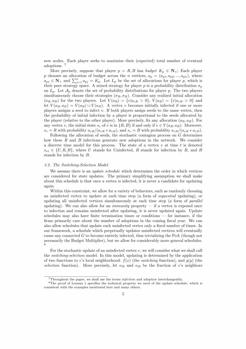
Regarding this form for f , for r = 1 we have linear adoption. For r < 1 we have fconcave, corresponding to cases in which the probability of adoption rises quickly withonly a small fraction of adopting neighbors, but then saturates or levels off with largerfractions of adopting neighbors. In contrast, for r > 1 we have f convex, which at verylarge values of r can begin to approximate threshold adoption behavior — the probabilityof adoption remains small until some fraction of neighbors has adopted, then rises rapidly.See Figure 1.

Regarding this form for g, which is known as the Tullock contest function (Tullock(1980)), for s = 1 we have a (linear) voter model in which the probability of selection isproportional to local market share. For s < 1 we have what we shall call an equalizingg, by which we mean that selection of the minority party in the neighborhood is favoredrelative to the linear voter model g(y) = y; and for s > 1 we have a polarizing g, meaningthat the minority party is disfavored relative to the linear model. As s approaches 0,we approach the completely equalizing choice g ≡ 1/2, and as s approaches infinity, weapproach the completely polarizing winner-take-all g; see Figure 1.

These parametric families of switching and selection functions will play an importantrole in illustrating our general results. The appendix discussed a few technology adop-tion examples which are (qualitatively) covered by these families of functions. In the

8

Figure 1: Left: Plots of f(x) = xr for varying choices of r, including r = 1 (linear, red line), r < 1(concave), and r > 1 (convex). Right: Plots of g(y) = ys/(ys + (1 − y)s) for varying choices of s,including s = 1 (linear, red line), s < 1 (equalizing), and s > 1 (polarizing).

proofs of some of our results, it will sometimes be convenient to use a more general adop-tion function formulation with some additional technical conditions that are met by ourswitching-selection formulation. We will refer to this general, single-step model as thegeneralized adoption function model. In this model, if the local fractions of Red and Blueneighbors are αR and αB , the probability that we update the vertex with an R infectionis h(αR, αB) for some adoption function h with range [0, 1], and symmetrically the proba-bility of B infection is thus h(αB , αR). Let us use H(αR, αB) = h(αR, αB)+h(αB , αR) todenote the total infection probability under h. Note that we can still always decompose hinto a two-step process by defining the switching function to be f(αR, αB) = H(αR, αB)and defining the selection function to be

g(αR, αB) = h(αR, αB)/(h(αR, αB) + h(αB , αR))

which is the infection-conditional probability that R wins the infection. The switching-9

Figure 2: A sample graph G.

selection model is thus the special case of the generalized adoption function model inwhich H(αR, αB) = f(αR + αB) is a function of only αR + αB , and g(αR, αB) is afunction of only αR/(αR + αB).11

5. Examples

We provide a simple example showing the effect of the switching and selection func-tions, and the relative budgets of the players, on the equilibrium solution.

Consider the graph G illustrated in figure 2. Here N is chosen to be much largerthan (KR + KB). The update schedule we consider for this example is a single parallelupdate, however all the claims hold as well for any other update schedule in which everynode is updated exactly once. We also assume f(x) = xα, therefore f is convex whenα > 1, it is linear when α = 1, and it is concave when 0 ≤ α ≤ 1.

Observe that in an equilibrium on G, no seed is ever placed on the bottom layerof a component, therefore in order to simplify the statement of our claims, we say aplayer chooses one component, when she puts some of her seeds on the top layer of thatcomponent.

We claim that the following propositions hold:

• If f is concave, regardless of the form of g (whether linear, equalizing or punishing),the only equilibrium is the case where players put each of their seeds in a separatecomponent of G, i.e. there is no more than one seed in each component.

Here is the reason: Suppose not and in the equilibrium, r + b > 1 seeds are on thetop layer of one of the components, say Ci, where r is the number of Red seeds,and b is the number of blue seeds on Ci. We know that the expected number ofinfections in that component is T = N ×f( r+b

KR+KB). Let us define the “fair share”

11While the decomposition in terms of a switching function and a selection function accommodates afairly wide range of adoption dynamics there are some cases which are ruled out. Consider the choiceh(x, y) = x(1 − y2); it is easily verified that the total probability of adoption H(x, y) is increasing in xand y. But H(x, y) clearly cannot be expressed as a function of the form f(x+y). Similarly, it is easy toconstruct an adoption function that is not only not decomposable, but violates monotonicity. Imagineconsumers that prefer to adopt the majority choice in their neighborhood, but will only adopt once theirlocal neighborhood market is sufficiently settled in favor of one or the other product. The probability oftotal adoption may then be higher with x = 0.2, y = 0 as compared to x = y = 0.4.

10

of Red and Blue in Ci to be T × rr+b and T × b

r+b respectively. Observe thatregardless of g, there exist a player (say Red) whose actual share is less than orequal to her fair share. Now note that if the Red player moves her seeds from Ciand put each of them in a separate empty component, her expected payoff wouldbe N × f( 1

KR+KB)× r which we claim is larger than her current payoff. Note that

Red’s current payoff is at most N × f( r+bKR+KB

)× rr+b , so it suffices to show that:

N × f(1

KR +KB)× r > N × f(

r + b

KR +KB)× r

r + b

To prove the above holds, we note that it is equivalent to:

f(1

KR +KB) > f(

r + b

KR +KB)× 1

r + b

and the last equation holds due to concavity of f . This means that the Red playercan increase her payoff by moving her seeds from Ci to empty components of G,which contradicts the assumption of being in an equilibrium.

• If f is convex and g is linear, the only equilibrium is the case where both playersput all of their seeds in the same component.

The reason the above holds is as follows: When g is linear every player gets her fairshare (as defined earlier) of the total number of infections in each component. Nownote that every time a player moves her seeds from one component to a componentwith larger number of seeds on, due to the convexity of f , she is increasing thetotal number of her infections in G. To be more precise, suppose there are r + bseeds on component Ci and r′ + b′ seeds on component Cj where r + b ≥ r′ + b′.The payoff per seed for Red in Ci and Cj are:

N × f(r + b

KR +KB)/(r + b)

and

N × f(r′ + b′

KR +KB)/(r′ + b′)

respectively. By moving her seeds from Cj to Ci, the payoff per seed for Red willbecome:

N × f(r + b+ r′

KR +KB)/(r + b+ r′)

Which is larger than the previous two due to the convexity of f . This means thatthe best response to a given opponent strategy is always to find the componentwith the largest number of seeds, and put all the seeds there. Therefore the onlyequilibrium will be the case where all the seeds are on the same component.

11

• If f is convex, g is equalizing, and KR

KB= 1, depending on whether f or g has a

stronger impact, the equilibrium solution can vary. In other words the convexity off makes players put their seeds close to one another to increase the total number ofinfections, whereas the equalizing effect of g makes them avoid having the majorityof seeds in any component. Therefore players face a trade-off that results in variousequilibrium solutions.

If we fix g and make f very convex then the only equilibrium will be the case whereboth players put all of their seeds in the same component. The reason is thatadding a seed to a larger group of seeds increases the total number of infections bya relatively large amount that makes the unfair share acceptable.

On the other hand, if we fix g and make f less and less convex, not being themajority becomes a more important condition to satisfy. If f is linear for example,one equilibrium is the case where Red and Blue seeds are paired with each otheron KR different components (it is very easy to verify this: first note that movingseeds does not change the total number of infections in G; second, moving a seedto an empty component clearly does not add to the number of infections one canget –although the assignment remains stable, and third and last, moving a seed toa component that already has a few seeds on, just makes the corresponding playerthe majority on that component, which is not desirable).

• If f is convex, g is punishing, and KR

KB= 1, one equilibrium is the case where both

players put all of their seeds in the same component. Note that in this case theconvexity of f makes players put their seeds close to each other. In addition thepunishing effect of g makes being the majority desirable. Now it is easy to seethat the above case is an equilibrium: given the opponent puts all her seeds on onecomponent, the best one can do is to add her seeds to the same component.

If f is too convex, then the above will be the only equilibrium. As f gets closer tolinear, more stable solutions emerge as well.

• If f is convex, g is equalizing, and KR

KB> 1, again various solutions are possible

depending on f and g.

If f is very convex the only equilibrium is the case where both players put all oftheir seeds in the same component. As f becomes closer to linear, the red playerplays as diverse as she can by putting each of her seeds on different components ofG to avoid becoming the majority in any component. The best response of Bluethen would be to play each of her seeds in a different component (not necessarilyempty of Red seeds).

• If f is convex, g is punishing, and KR

KB> 1, then the Red (larger budget) player

tries to gather her seeds close to each other and the Blue player’s seeds, as it makesboth the total infections and her share, larger at the same time. The blue playeron the other hand avoids playing close to Red seeds, unless f is very convex and hegets very few infections in case of not playing close to Red seeds. Thus dependingon which function has a stronger impact, the equilibrium solution may be different.

If f is very convex the only equilibrium is the case where both players put all of theirseeds in the same component. As f becomes closer to linear, the blue player can

12

play farther from Red. If f is linear for example, there is no pure Nash equilibrium,but the high-level strategies of the players would be to place their seeds in a waythat they become the majority in as many components as they can.

The general points the above example makes are the following:

1. Fixing g, As f becomes more and more concave, each player tends to keep theirseeds far from one another and also from the opponent’s seeds.

2. Fixing g, the more convex f gets, the more the players tendency to keep their seedsclose to each other and also close to the opponent’s seeds.

3. Fixing f , the more equalizing g gets, the player with smaller budget tends toplay near the large-budget player, while the large budget player avoids being themajority. The quantity KR

KBindicates how effective this is: if it is small, e.g. 1, g

does not affect the equilibrium greatly.

4. Fixing f , the more punishing g gets, the player with larger budget tends to playnear the small-budget player, while the small budget player avoids playing close toher opponent. The quantity KR

KBindicates how effective this is: if it is small, e.g.

1, g does not affect the equilibrium greatly.

Here we chose a symmetric network to be able to see the pure effect of f , g and KR

KB

on the equilibrium. When the underlying network is not symmetric players face anothertrade-off that rises due to the effect of the network structure. For example although it isin general true that the more concave f gets, the more far apart players put their seeds,this does not hold in all networks, e.g. if the network has only a few important vertices,then players still play near each other to compete for those high impact vertices.

6. Results: Price of Anarchy and Price of Stability

We first develop a number of examples to illustrate the trade-offs and the issues withregard to costs of decentralization. We then state and prove a theorem providing generalconditions in the switching-selection model under which the Price of Anarchy is boundedby a constant that is independent of the size and structure of the graph G. The simplestcharacterization is that f being any concave function (satisfying f(0) = 0, f(1) = 1 andf increasing), and g being the linear voter function g(y) = y leads to bounded PoS; butwe shall see the conditions allow for certain combinations of concave f and nonlinearg as well. We then prove a lower bound showing that the concavity of f is requiredfor bounded PoS in a very strong sense — a small amount of convexity can lead tounbounded PoS.

6.1. PoA: Examples

Suppose that budgets of the firms are KR = KB = 1, and the update rule is suchthat all vertices are updated only once. The network contains two connected componentswith 10 vertices and 100 vertices, respectively. In each component there are 2 influentialvertices, each of which is connected to the other 8 and 98 vertices, respectively. So incomponent 1, there are 16 directed links while in component 2 there are 196 directedlinks in all.

13

• Suppose that the switching function and the selection function are both linear,f(x) = x and g(y) = y. Then there is a unique equilibrium in which players placetheir seeds on distinct influential vertices of component 2. The total infection isthen 100 and this is the maximum number of infections possible with 2 seeds. Sohere the PoA is 1.

• Let us now alter the switching function such that f(1/2) = ε for some ε < 1/25(keeping f(1) = 1, as always), but retain the selection function to be g(y) = y.Now there also exists an equilibrium in which the firms locate on the influentialvertices of component 1. In this equilibrium payoffs to each player are equal to 5.Observe that for ε < 1/25, a deviation to the other component is not profitable: ityields an expected payoff equal to 1 + ε × 98, and this is strictly smaller than 5.Since it is still possible to infect component 2 with 2 seeds, the PoA is 10. Hereinefficiency is created by a coordination failure of the players.

• Finally, suppose there is only one component with 110 vertices, with 2 influentialvertices and 108 vertices receiving directed links. Then equilibrium under bothswitching functions considered above will involve firms locating at the 2 influentialvertices and this will lead to infection of all vertices. So the PoA is 1, irrespectiveof whether the switching function is linear f(x) = x or whether f(1/2) < 1/25.

Thus for a fixed network, updating rule and selection function, variations in theswitching function can generate large variations in the PoA. Similarly, for fixed updaterule and switching and selection functions, a change in the network structure yields verydifferent PoA.

Theorem 1 provides a set of sufficient conditions on switching and selection function,under which the PoA is uniformly bounded from above. Theorem 2 shows how evensmall violations of these conditions can lead to arbitrarily high PoA.

6.2. PoA: Upper Bound

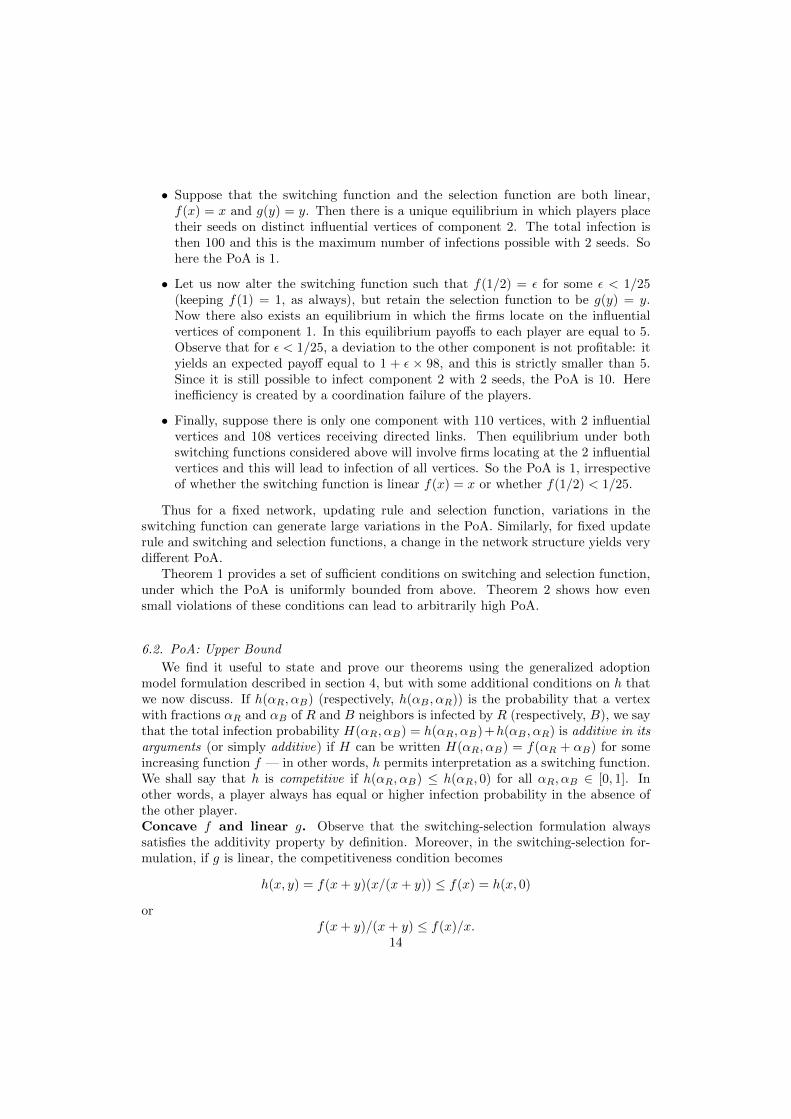
We find it useful to state and prove our theorems using the generalized adoptionmodel formulation described in section 4, but with some additional conditions on h thatwe now discuss. If h(αR, αB) (respectively, h(αB , αR)) is the probability that a vertexwith fractions αR and αB of R and B neighbors is infected by R (respectively, B), we saythat the total infection probability H(αR, αB) = h(αR, αB)+h(αB , αR) is additive in itsarguments (or simply additive) if H can be written H(αR, αB) = f(αR + αB) for someincreasing function f — in other words, h permits interpretation as a switching function.We shall say that h is competitive if h(αR, αB) ≤ h(αR, 0) for all αR, αB ∈ [0, 1]. Inother words, a player always has equal or higher infection probability in the absence ofthe other player.Concave f and linear g. Observe that the switching-selection formulation alwayssatisfies the additivity property by definition. Moreover, in the switching-selection for-mulation, if g is linear, the competitiveness condition becomes

h(x, y) = f(x+ y)(x/(x+ y)) ≤ f(x) = h(x, 0)

orf(x+ y)/(x+ y) ≤ f(x)/x.

14

This condition is satisfied by the concavity of f . We will later see that the followingtheorem also applies to certain combinations of concave f and nonlinear g. The firsttheorem can now be stated.

Theorem 1. If the adoption function h(αR, αB) is competitive and H is additive in itsarguments, then Price of Anarchy is at most 4 for any graph G.

Proof We establish the theorem via a series of lemmas and inequalities that can besummarized as follows. Let (S∗R, S

∗B) be an initial allocation of infections that gives the

maximum joint payoff, and let (SR, SB) be a pure12 Nash equilibrium with SR beingthe larger set of seeds, so KR = |S∗R| = |SR| ≥ KB = |S∗B | = |SB |. We first establisha general lemma (Lemma 1) that implies that the set S∗R alone (without S∗B present)must yield payoffs close to the maximum joint payoff (Corollary 1). The proof involvesthe construction of a coupled stochastic process technique we employ repeatedly in thepaper. 13 We then contemplate a deviation by the Red player to (S∗R, SB). Anothercoupling argument (Lemma 2) establishes that the total payoffs for both players under(S∗R, SB) must be at least those for the Red player alone under (S∗R, ∅). This meansthat under (S∗R, SB), one of the two players must be approaching the maximum jointinfections. If it is Red, we are done, since Red’s equilibrium payoff must also be thislarge. If it is Blue, Lemma 1 implies that Blue could still get this large payoff even afterthe departure of Red. Next we invoke Lemma 2 to show that total eventual payoff toboth players under (SR, SB) must exceed this large payoff accruing to Blue, proving thetheorem.

Lemma 1. Let AR and AB be any sets of seed vertices for the two players. Then if his competitive,

E[χR|(AR, ∅)] ≥ E[χR|(AR, AB)]

andE[χB |(∅, AB)] ≥ E[χB |(AR, AB)].

Proof We provide the proof for the first statement involving χR; the proof for χB isidentical. We introduce a simple coupled simulation technique that we shall appeal toseveral times throughout the paper. Consider the stochastic dynamical process on Gunder two different initial conditions: both AR and AB are present (the joint process,denoted (AR, AB) in the conditioning in the statement of the lemma); and only theset AR is present (the solo Red process, denoted (AR, ∅)). Our goal is to define a newstochastic process on G, called the coupled process, in which the state of each vertex vwill be a pair < Xv, Yv >. We shall arrange that Xv faithfully represents the state of

12The extension to mixed strategies is straightforward and omitted.13The theorem includes concave (and therefore sub-modular) f and makes extensive use of coupling

arguments to prove local-to-global effects (of which Lemmas 1 and 2 are examples); this bears a similarityto the work of Mossel and Roch [21], and it has been suggested that our proofs might be simplified byappeal to their results. However, we have not been able to apply their results in our context. Two featuresof our framework seem to make direct application difficult: first, the important role of competitive effects,which is explicit in Lemma 1; and second, the variety of updating schedules we consider appear not becovered by the general threshold model which underlies the Mossel and Roch analysis. While we suspectmore direct relationships might be possible in special cases, here we provide proofs specific to our model.

15

a vertex in the joint process, and Yv the state in the solo Red process. However, thesestate components will be correlated or coupled in a deliberate manner. More precisely,we wish to arrange the coupled process to have the following properties:

1. At each step, and for any vertex state < Xv, Yv >, Xv ∈ {U,R,B} and Yv ∈ {U,R}.

2. Projecting the states of the coupled process onto either component faithfully yieldsthe respective process. Thus, if < Xv, Yv > represents the state of vertex v in thecoupled process, then the {Xv} are stochastically identical to the joint process, andthe {Yv} are stochastically identical to the solo Red process.

3. At each step, and for any vertex state < Xv, Yv >, Xv = R implies Yv = R.

Note that the first two properties are easily achieved by simply running independent jointand solo Red processes. But this will violate the third property, which yields the lemma,and thus we introduce the coupling.

For any vertex v, we define its initial coupled process state < Xv, Yv > as follows:Xv = R if v ∈ AR, Xv = B if v ∈ AB , and Xv = U otherwise; and Yv = R if v ∈ AR,and Yv = U otherwise. It is easily verified that these initial states satisfy Properties 1and 3 above, thus encoding the initial states of the two separate processes.

Assume for now that the first vertex 14 v to be updated in the X and Y processesare the same — i.e. the same vertices are updated in both the joint and solo updateschedules, which may in general depend on the state of the network in each. We nowdescribe the coupled updates of v. Let αRv denote the fraction of v’s neighbors w suchthat Xw = R, and αBv the fraction such that Xw = B. Note that by the initialization ofthe coupled process, αRv is also equal to the fraction of Yw = R (which we denote αRv ).

In the joint process, the probability that v is updated to R is h(αRv , αBv ), and to B is

h(αBv , αRv ). In the solo Red process, the probability that v is updated to R is h(αRv , 0),

which by competitiveness is greater than or equal to h(αRv , αBv ).

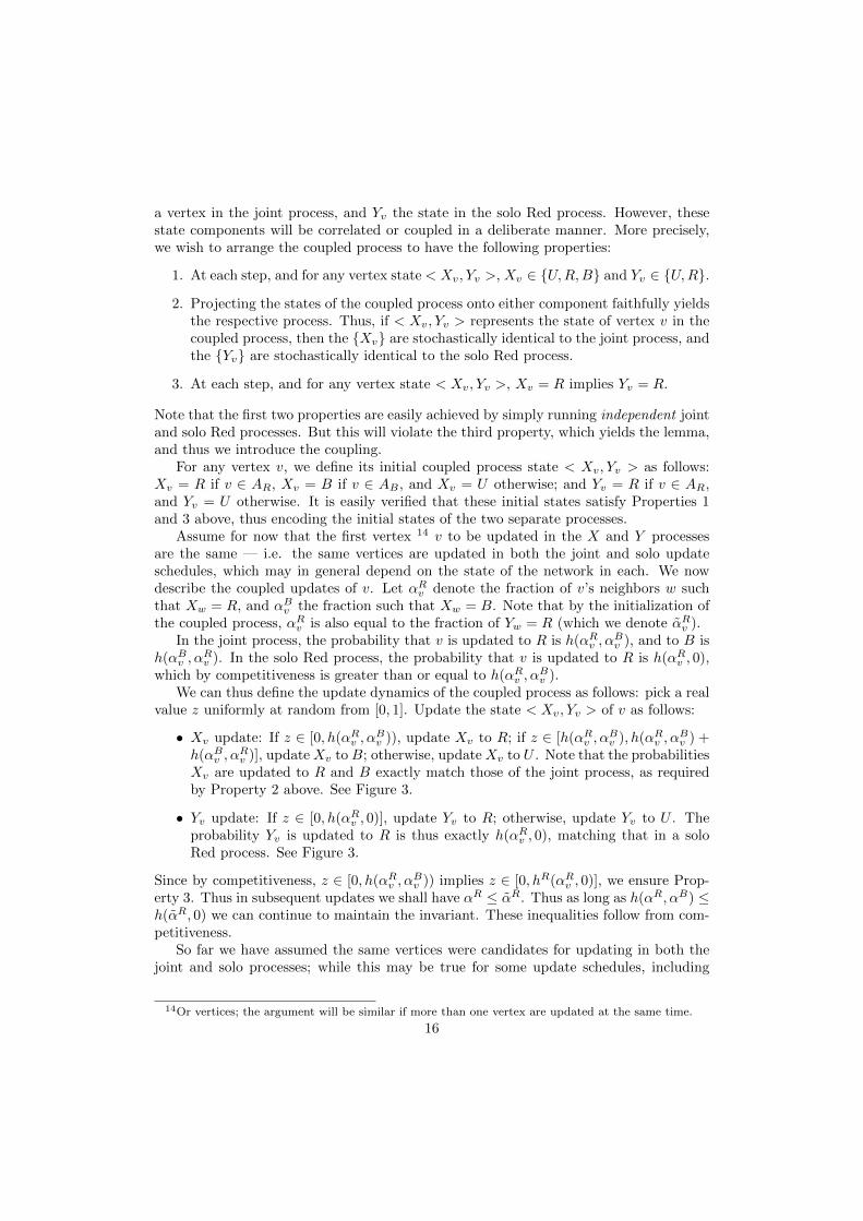
We can thus define the update dynamics of the coupled process as follows: pick a realvalue z uniformly at random from [0, 1]. Update the state < Xv, Yv > of v as follows:

• Xv update: If z ∈ [0, h(αRv , αBv )), update Xv to R; if z ∈ [h(αRv , α

Bv ), h(αRv , α

Bv ) +

h(αBv , αRv )], updateXv to B; otherwise, updateXv to U . Note that the probabilities

Xv are updated to R and B exactly match those of the joint process, as requiredby Property 2 above. See Figure 3.

• Yv update: If z ∈ [0, h(αRv , 0)], update Yv to R; otherwise, update Yv to U . Theprobability Yv is updated to R is thus exactly h(αRv , 0), matching that in a soloRed process. See Figure 3.

Since by competitiveness, z ∈ [0, h(αRv , αBv )) implies z ∈ [0, hR(αRv , 0)], we ensure Prop-

erty 3. Thus in subsequent updates we shall have αR ≤ αR. Thus as long as h(αR, αB) ≤h(αR, 0) we can continue to maintain the invariant. These inequalities follow from com-petitiveness.

So far we have assumed the same vertices were candidates for updating in both thejoint and solo processes; while this may be true for some update schedules, including

14Or vertices; the argument will be similar if more than one vertex are updated at the same time.

16

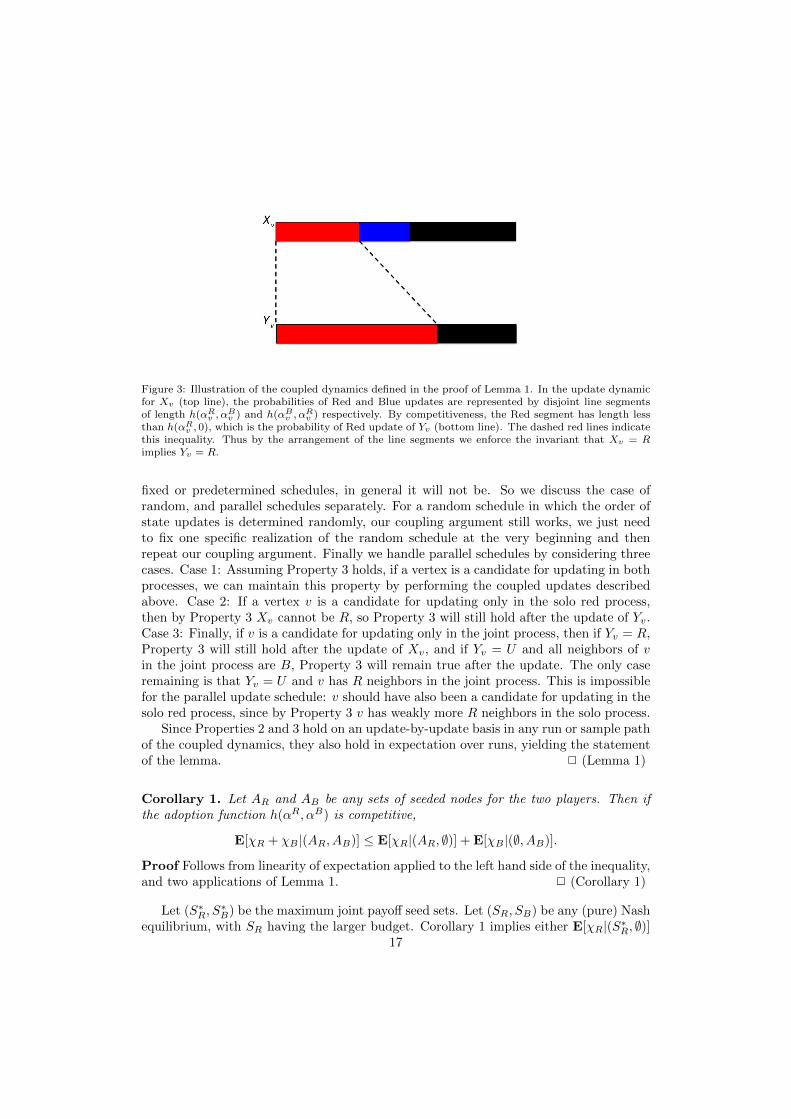
Figure 3: Illustration of the coupled dynamics defined in the proof of Lemma 1. In the update dynamicfor Xv (top line), the probabilities of Red and Blue updates are represented by disjoint line segmentsof length h(αR

v , αBv ) and h(αB

v , αRv ) respectively. By competitiveness, the Red segment has length less

than h(αRv , 0), which is the probability of Red update of Yv (bottom line). The dashed red lines indicate

this inequality. Thus by the arrangement of the line segments we enforce the invariant that Xv = Rimplies Yv = R.

fixed or predetermined schedules, in general it will not be. So we discuss the case ofrandom, and parallel schedules separately. For a random schedule in which the order ofstate updates is determined randomly, our coupling argument still works, we just needto fix one specific realization of the random schedule at the very beginning and thenrepeat our coupling argument. Finally we handle parallel schedules by considering threecases. Case 1: Assuming Property 3 holds, if a vertex is a candidate for updating in bothprocesses, we can maintain this property by performing the coupled updates describedabove. Case 2: If a vertex v is a candidate for updating only in the solo red process,then by Property 3 Xv cannot be R, so Property 3 will still hold after the update of Yv.Case 3: Finally, if v is a candidate for updating only in the joint process, then if Yv = R,Property 3 will still hold after the update of Xv, and if Yv = U and all neighbors of vin the joint process are B, Property 3 will remain true after the update. The only caseremaining is that Yv = U and v has R neighbors in the joint process. This is impossiblefor the parallel update schedule: v should have also been a candidate for updating in thesolo red process, since by Property 3 v has weakly more R neighbors in the solo process.

Since Properties 2 and 3 hold on an update-by-update basis in any run or sample pathof the coupled dynamics, they also hold in expectation over runs, yielding the statementof the lemma. 2 (Lemma 1)

Corollary 1. Let AR and AB be any sets of seeded nodes for the two players. Then ifthe adoption function h(αR, αB) is competitive,

E[χR + χB |(AR, AB)] ≤ E[χR|(AR, ∅)] + E[χB |(∅, AB)].

Proof Follows from linearity of expectation applied to the left hand side of the inequality,and two applications of Lemma 1. 2 (Corollary 1)

Let (S∗R, S∗B) be the maximum joint payoff seed sets. Let (SR, SB) be any (pure) Nash

equilibrium, with SR having the larger budget. Corollary 1 implies either E[χR|(S∗R, ∅)]17

or E[χB |(∅, S∗B)] is at least as great as E[χR + χB |(S∗R, S∗B)]/2; so assume without lossof generality 15 that E[χR|(S∗R, ∅)] ≥ E[χR + χB |(S∗R, S∗B)]/2. Let us now contemplatea unilateral deviation of the Red player from SR to S∗R, in which case the strategies are(S∗R, SB). In the following lemma we show that the total number of eventual adoptionsfor the two players is larger than adoptions accruing to a single player under solo seeding.

Lemma 2. Let AR and AB be any sets of seeded nodes for the two players. If H isadditive,

E[χR + χB |(AR, AB)] ≥ E[χR|(AR, ∅)].

Proof We employ a coupling argument similar to that in the proof of Lemma 1. Wedefine a stochastic process in which the state of a vertex v is a pair < Xv, Yv > in whichthe following properties are obeyed:

1. At each step, and for any vertex state < Xv, Yv >, Xv ∈ {R,B,U} and Yv ∈{R,U}.

2. Projecting the state of the coupled process onto either component faithfully yieldsthe respective process. Thus, if < Xv, Yv > represents the state of vertex v inthe coupled process, then the {Xv} are stochastically identical to the joint process(AR, AB), and the {Yv} are stochastically identical to the solo Red process (AR, ∅).

3. At each step, and for any vertex state < Xv, Yv >, Yv = R implies Xv = R orXv = B.

We initialize the coupled process in the obvious way: if v ∈ AR then Xv = R, ifv ∈ AB then Xv = B, and Xv = U otherwise; and if v ∈ AR then Yv = R, andYv = U otherwise. Let us fix a vertex v to update, and let αRv , α

Bv denote the fraction of

neighbors w of v with Xw = R and Xw = B respectively, and let αRv denote the fractionwith Yw = R. Initially we have αRv = αRv .

We assume the vertex or vertices v to be updated in the X and Y processes are thesame; the fact that the update schedules may cause these sets to differ is handled inthe same way as in the proof of Lemma 1. On the first update of v in the joint process(AR, AB), the total probability infection by either R or B is

H(αRv , αBv ) = h(αRv , α

Bv ) + h(αBv , α

Rv ).

In the solo process (AR, ∅), the probability of infection by R is h(αRv , 0) ≤ h(αRv , 0) +h(0, αRv ) = H(αRv , 0) ≤ H(αRv , α

Bv ) where the last inequality follows by the additivity of

H.We thus define the update dynamics in the coupled process as follows: pick a real

value z uniformly at random from [0, 1]. Update < Xv, Yv > as follows:

15If this does not hold, instead of (S∗R, S

∗B), consider the seed set (T ∗

R, T∗B) in which T ∗

R = S∗B∪(S∗

R−S)and T ∗

B = S where S is any subset of S∗R of size KB for which S ∪S∗

B ∪ (S∗R −S) = S∗

R ∪S∗B . Note that

this new seed set also maximize the joint payoff.

18

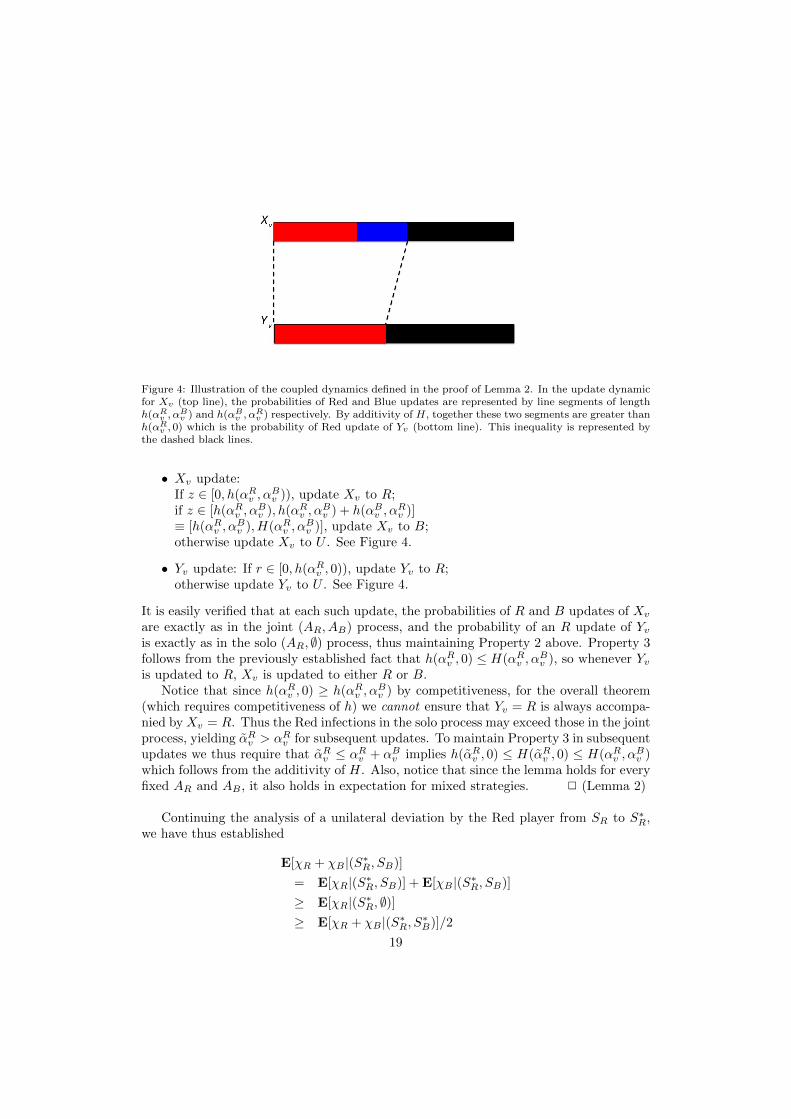
Figure 4: Illustration of the coupled dynamics defined in the proof of Lemma 2. In the update dynamicfor Xv (top line), the probabilities of Red and Blue updates are represented by line segments of lengthh(αR

v , αBv ) and h(αB

v , αRv ) respectively. By additivity of H, together these two segments are greater than

h(αRv , 0) which is the probability of Red update of Yv (bottom line). This inequality is represented by

the dashed black lines.

• Xv update:If z ∈ [0, h(αRv , α

Bv )), update Xv to R;

if z ∈ [h(αRv , αBv ), h(αRv , α

Bv ) + h(αBv , α

Rv )]

≡ [h(αRv , αBv ), H(αRv , α

Bv )], update Xv to B;

otherwise update Xv to U . See Figure 4.

• Yv update: If r ∈ [0, h(αRv , 0)), update Yv to R;otherwise update Yv to U . See Figure 4.

It is easily verified that at each such update, the probabilities of R and B updates of Xv

are exactly as in the joint (AR, AB) process, and the probability of an R update of Yvis exactly as in the solo (AR, ∅) process, thus maintaining Property 2 above. Property 3follows from the previously established fact that h(αRv , 0) ≤ H(αRv , α

Bv ), so whenever Yv

is updated to R, Xv is updated to either R or B.Notice that since h(αRv , 0) ≥ h(αRv , α

Bv ) by competitiveness, for the overall theorem

(which requires competitiveness of h) we cannot ensure that Yv = R is always accompa-nied by Xv = R. Thus the Red infections in the solo process may exceed those in the jointprocess, yielding αRv > αRv for subsequent updates. To maintain Property 3 in subsequentupdates we thus require that αRv ≤ αRv + αBv implies h(αRv , 0) ≤ H(αRv , 0) ≤ H(αRv , α

Bv )

which follows from the additivity of H. Also, notice that since the lemma holds for everyfixed AR and AB , it also holds in expectation for mixed strategies. 2 (Lemma 2)

Continuing the analysis of a unilateral deviation by the Red player from SR to S∗R,we have thus established

E[χR + χB |(S∗R, SB)]

= E[χR|(S∗R, SB)] + E[χB |(S∗R, SB)]

≥ E[χR|(S∗R, ∅)]≥ E[χR + χB |(S∗R, S∗B)]/2

19

where the equality is by linearity of expectation, the first inequality follows from Lemma 2,and the second inequality from Corollary 1. Thus at least one of E[χR|(S∗R, SB)] andE[χB |(S∗R, SB)] must be at least E[χR + χB |(S∗R, S∗B)]/4.

If E[χR|(S∗R, SB)] ≥ E[χR+χB |(R∗, B∗)]/4, then since (SR, SB) is Nash, E[χR|(SR, SB)] ≥E[χR + χB |(S∗R, S∗B)]/4, and the theorem is proved. The only remaining case is whereE[χB |(S∗R, SB)] ≥ E[χR + χB |(S∗R, S∗B)]/4. But Lemma 1 has already established thatE[χB |(∅, SB)] ≥ E[χB |(S∗R, SB)], and we have E[χR+χB |(SR, SB)] ≥ E[χB |(∅, SB)] fromLemma 2. Combining, we have the following chain of inequalities:

E[χR + χB |(SR, SB)] ≥ E[χB |(∅, SB)]

≥ E[χB |(S∗R, SB)]

≥ E[χR + χB |(S∗R, S∗B)]/4

thus establishing the theorem. 2 (Theorem 1)

Concave f , non-linear g. Recall that the switching-selection formulation in whichf is concave and g is linear satisfies the hypothesis of the Theorem above. But Theorem 1also provides more general conditions for bounded PoA in the switching-selection model.For example, suppose we consider switching functions of the form f(x) = xr for r ≤ 1(thus yielding concavity) and selection functions of the Tullock contest form g(y) =ys/(ys + (1− y)s), as discussed in Section 3.2. Letting a and b denote the local fractionof Red and Blue neighbors for notational convenience, this leads to an adoption functionof the form h(a, b) = (a+ b)r/(1 + (b/a)s). The condition for competitiveness is

h(a, 0)− h(a, b) = ar − (a+ b)r/(1 + (b/a)s) ≥ 0.

Dividing through by (a+ b)r yields

(a/(a+ b))r − 1/(1 + (b/a)s)

= 1/(1 + (b/a))r − 1/(1 + (b/a)s) ≥ 0.

Making the substitution z = b/a and moving the second term to the right-hand sidegives

1/(1 + z)r ≥ 1/(1 + zs).

Thus competitiveness is equivalent to the condition 1 + zs ≥ (1 + z)r for all z ≥ 0. Itis not difficult to show that any s ∈ [r, 1] will satisfy this condition. In other words, themore concave f is (i.e. the smaller r is), the more equalizing g can be (i.e. the smaller scan be) while maintaining competitiveness. By Theorem 1 we have thus shown:

Corollary 2. Let the switching function be f(x) = xr for r ≤ 1 and let g(y) = ys/(ys +(1− y)s) be the selection function. Then as long as s ∈ [r, 1], the Price of Anarchy is atmost 4 for any graph.

6.3. PoS: Lower Bound

We now show that concavity of the switching function is required in a very strongsense — essentially, even a slight convexity leads to unbounded PoS.

20

Theorem 2. Let the switching function be f(x) = xr for any r > 1, and let the selectionfunction be linear g(y) = y. Then for any V > 0, there exists a graph G for which thePrice of Stability is greater than V .

Proof The idea is to create a layered, directed graph whose dynamics rapidly amplifythe convexity of f . We show that for any arbitrary natural number V , there is a graphin which the price of stability is larger than V .

Suppose KR = 1 and KB = K where K > V . Let ε = 1(K+1)4 . Since r > 1 and

KK+1 < 1 we can choose a constant l such that ( K

K+1 )rl

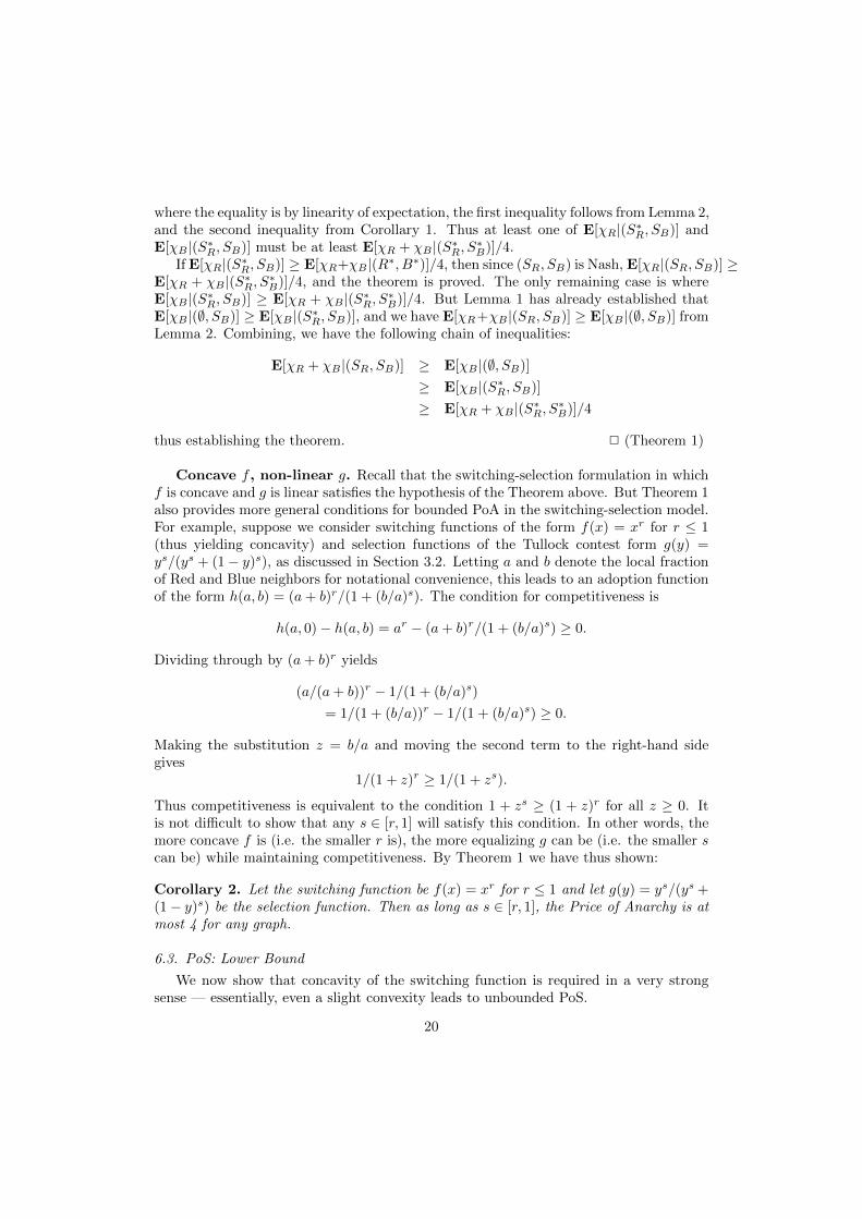
< ε.Consider the graph G consisting of two components A,B depicted in figure 5. Com-

ponent B is a (l+2)-layered graph, where the first layer has (K+1) vertices, the second,third, and the (l + 1)th layer all have M vertices with M = K+1

ε = (K + 1)5, and thelast layer has N vertices where N is much larger than K (say N = O(10K)). A node inlayer i (1 ≤ i ≤ l) of component B has an outgoing edge to every node in layer (i + 1).Component A = K1,Q is a complete bipartite graph with Q = Ml+N

K+1 + 1.When the first layer of B is entirely covered with seeds i.e. all the (K + 1) seeds are

placed on u1, ..., uK+1, the eventual number of infected nodes in that component is equalto K+1+ lM+N . We claim that this case maximizes the eventual number of infections:First observe that if there are less than (K + 1) seeds in component B, it is not possiblefor infections in its last layer to be larger than εN : If the seeds are on the first layer, the

number of infections in the last layer would be ( KK+1 )r

l ×N which is less than εN due tothe way we chose l. Also if the seeds are on a layer other than the first layer of B, thenno more than K

M < ε fraction of that layer can be infected which results in a numberof infections less than εN in the last layer. Therefore it is not possible for number ofinfections in the last layer of B to be larger than εN when there are less than (K + 1)initial seeds put on component B. (We note that the claims with regard to infections are‘approximate’: the actual infections will converge to these approximations, as the layersget large).

Since the total number of infections in component A cannot be greater than thenumber of nodes in it i.e. Ml+N

K+1 + 2, the expected total number of infections in G whenthe first layer of B is not entirely covered with seeds would be less than εN + lM +K +Ml+NK+1 + 2. The later is less than K + 1 + lM + N once N is chosen sufficiently large.

Therefore we can conclude that the expected number of infections is maximized when allthe seeds are on the first layer of component B.

Note that the assignment that maximizes the expected number of infections is not anequilibrium since in that case the Red player gets (in expectation) Ml+N

K+1 + 1 infections,and therefore she is better off by moving her only seed to u where she gets slightly more,i.e. Ml+N

K+1 + 2 infections in expectation.Next we proceed to find the equilibrium: we claim that regardless of the strategy

of the Blue player, the dominant strategy for the Red player is to put her only seed onu. To prove this we consider all possible cases: Above we discussed that if the Blueplayer plays entirely on component B, the Red player prefers to place her seed on u.In other cases where the Blue player has a few seeds in A and a few seeds in B, if theRed player puts her seed on u, in the worst case (which is the case where all the Blueseeds are also put on u), she gets in expectation Ml+N+K+1

(K+1)2 infections. Whereas if she

plays in component B, what she gets is bounded by the maximum infections that can

21

Figure 5: A graph with PoS greater than K

possibly be achieved in B with K seeds which is, as argued before, at most εN + lM +K(The later is equal to N

(k+1)4 + lM +K). Thus when N is much larger than K, we haveMl+N+K+1

(K+1)2 > N(k+1)4 + lM + K, which means the better strategy for the Red player is

to stay on u, even in the worst case where there is a heavy competition for getting thatnode.

Now that we showed selecting u as the seed set is the dominant strategy for the Redplayer, it is easy to see the best move for the Blue player is to put all her seeds on u aswell. Suppose not and the Blue player has z < K seeds on u and K − z > 0 seeds inB. For each seed that Blue moves from component B to u, she increase her expectedinfection in component A by at least ( K

K+1 −K−1K ) × Ml+N

(K+1) ≥1

(K+1)2 ×Ml+N(K+1) (which

is equal to Ml+N(K+1)3 ), while in the component B the expected number of infections she is

losing at most εN + lM + K (which is equal to N(k+1)4 + lM + K). Since N � K it is

always beneficial for the Blue player to move her seeds from component B to u. Thismeans that the only equilibrium is the case where all the seeds are placed on u.

As the result of above, the price of stability for this network is at least:

Ml +N + (K + 1)Ml+N+(K+1)

K+1 + 1

It is very easy to see that by choosing N sufficiently large, the above can get arbitrarilyclose to (K + 1) which is larger than V . This completes the proof.

2

Combining Theorem 1 and Theorem 2, we note that for f(x) = xr and linear g weobtain the following sharp threshold result:

22

Corollary 3. Let the switching function be f(x) = xr, and let the selection function belinear, g(y) = y. Then:

• For any r ≤ 1, the Price of Anarchy (and as a result, Price of Stability) is at most4 for any graph G;

• For any r > 1 and any V , there exists a graph G for which the Price of Stability(and as a result, Price of Anarchy) is greater than V .

7. Results: Budget Multiplier

We start with some examples to illustrate the issues that arise. We then derivesufficient conditions for bounded Budget Multiplier, and show that violations of theseconditions can lead to unbounded Budget Multiplier.

8. Budget Multiplier: Examples

Suppose that budgets of the firms are KR = 1, KB = 2 and the update rule is suchthat all vertices are updated only once. The network contains 3 influential vertices, eachof which has a directed link to all the other n − 3 vertices, respectively. So there are3(n− 3) links in all. Let n� 3.

• Suppose the switching function and selection function are both linear, i.e., f(x) = xand g(y) = y. There is a unique equilibrium and in this equilibrium, players willplace their resources on distinct influential vertices. The (expected) payoffs toplayer R are n/3, while the payoffs to player B are 2n/3. So the Budget Multiplieris equal to 1.

• Next, suppose the switching function is convex with f(2/3) = 1/25, and the se-lection function g(y) is as in Tullock (1980). Suppose the two players place theirresources on the three influential vertices. The payoffs to R are g(1/3)n, while firmB earns g(2/3)n. Clearly this is optimal for firm B as any deviation can only lowerpayoffs. And, it can be checked that a deviation by firm R to one of the influentialvertices occupied by player B will yield a payoff of n/100 (approximately). So theconfiguration specified is an equilibrium so long as g(1/3) ≥ 1/100. The BudgetMultiplier is now (approximately) 50.

• Finally, suppose the network consists of ` equally-sized connected components. Ineach component, there is 1 influential vertex which has a directed link to each of the(n/`) − 1 other vertices. In equilibrium each player locates on distinct influentialvertices, irrespective of whether the switching function is convex or concave andwhether the Tullock selection function is linear (s = 1) or whether it is polarizing(s > 1). The Budget Multiplier is now equal to 1.

These examples show that for fixed network and updating rule, variations in theswitching and selection functions generate large variations in Budget Multiplier. More-over, for fixed switching and selection functions the payoffs depend crucially on thenetwork.

23

Theorem 3 provides a set of sufficient conditions on the switching and selection func-tion, under which the Budget Multiplier is uniformly bounded. Theorem 4 shows howeven small violations of these conditions can lead to arbitrarily high Budget Multiplier.Theorem 5 illustrates the role of concavity of the switching function in shaping the Bud-get Multiplier.

8.1. Budget Multiplier: Upper Bound

As in the PoA analysis, it will be technically convenient to return to the generalizedadoption function model. Recall that for PoA, competitiveness of h and additivity ofH were needed to prove upper bounds, but we didn’t require that the implied selectionfunction be linear. Here we introduce that additional requirement, and prove that the(pure strategy) Budget Multiplier is bounded.

Theorem 3. Suppose the adoption function h(αR, αB) is competitive, that H is additivein its arguments, and that the implied selection function is linear:

g(αR, αB) =h(αR, αB)

h(αR, αB) + h(αB , αB)= αR/(αR + αB)

Then the pure strategy Budget Multiplier is at most 2 for any graph G.16

Proof The proof borrows elements from the proof of Theorem 1, and introduces theadditional notion of tracking or attributing indirect infections generated by the dynamicsto specific seeds.

Consider any pure Nash equilibrium given by seed sets SR and SB in which |SR| =K > |SB | = L. For our purposes the interesting case is one in which

E[χR|(SR, SB)] ≥ E[χB |(SR, SB))]

and soE[χR|(SR, SB)] ≥ E[χR + χB |(SR, SB)]/2.

Since the adoption function is competitive and additive, Lemma 1 implies that

E[χR|(SR, ∅)] ≥ E[χR|(SR, SB)]

That is, the Red player only benefits from the departure of the Blue player.Let us consider the dynamics of the solo Red process given by (SR, ∅). We first intro-

duce a faithful simulation of these dynamics that also allows us to attribute subsequentinfections to exactly one of the seeds in SR; we shall call this process the attributionsimulation of (SR, ∅). Thus, let SR = {v1, . . . , vK} be the initial Red infections, and letus label vi by Ri, and label all other vertices U . All infections in the process will also beassigned one of the K labels Ri in the following manner: when updating a vertex v, wefirst compute the fraction αRv of neighbors whose current label is one of R1, . . . , RK , and

16The theorem actually holds for any equilibrium in which the player with the larger budget plays apure strategy; the player with smaller budget may always play mixed. It is easy to find cases with suchequilibria. The theorem also holds for general mixed strategies under certain conditions — for instance,when both f and g are linear and the larger budget is an integer multiple of the smaller.

24

with probability H(αRv , 0) = h(αRv , 0) + h(0, αRv ) we decide that an infection will occur(otherwise the label of v is updated to U). If an infection occurs, we simply choose aninfected neighbor of v uniformly at random, and update v to have the same label (whichwill be one of the Ri). It is easily seen that at every step, the dynamics of the (SR, ∅)process are faithfully implemented if we drop label subscripts and simply view any labelRi as a generic Red infection R. Furthermore, at all times every infected vertex has onlyone of the labels Ri. Thus if we denote the expected number of vertices with label Riby E[χRi |(SR, ∅)], we have E[χR|(SR, ∅)] =

∑Ki=1 E[χRi |(SR, ∅)]. Let us assume without

loss of generality that the labels Ri are sorted in order of decreasing E[χRi|(SR, ∅)].

We now consider the payoff to Blue under a deviation from SB to the set SB ={v1, . . . , vL} ⊂ SR — that is, the L “most profitable” initial infections in SR. Our goalis to show that the Blue player must enjoy roughly the same payoff from these L seedsas the Red player did in the solo attribution simulation.

Lemma 3.

E[χB |(SR, SB)] ≥ 1

2

L∑i=1

E[χRi|(SR, ∅)]

≥ L

2KE[χR|(SR, ∅)]

Proof The second inequality follows from

E[χR|(SR, ∅)] =

K∑i=1

E[χRi|(SR, ∅)],

established above, and fact that the vertices in SR are ordered in decreasing profitability.For the first inequality, we introduce coupled attribution simulations for the two processes(SR, ∅) (the solo Red process) and (SR, SB). For simplicity, let us actually examine(SR, ∅) and (SR− SB , SB); the latter joint process is simply the process (SR, SB), but inwhich the contested seeded nodes in SB are all won by the Blue player. (The proof forthe general (SR, SB) case is the same but causes the factor of 1/2 in the lemma.)

The coupled attribution dynamics are as follows: as above, in the solo Red process,for 1 ≤ i ≤ L, the vertex vi in SR is initially labeled Ri, and all other vertices are labeledU . In the joint process, the vertex vi is labeled Bi for i ≤ L (corresponding to the Blueinvasions of SR), while for L < i ≤ K the vertex vi is labeled Ri as before. Now at thefirst update vertex v, let αRv be the fraction of Red neighbors in the solo process, and letαRv and αBv be the fraction of Red and Blue neighbors, respectively, in the joint process.

Note that initially we have αRv = αRv + αBv . Thus by additivity H, the total prob-abilities of infection H(αRv , 0) and H(αRv , α

Bv ) in the two processes must be identical.

We thus flip a common coin with this shared infection probability to determine whetherinfections occur in the coupled process. If not, v is updated to U in both processes. Ifso, we now use a coupled attribution step in which we pick an infected neighbor of vat random and copy its label to v in both processes. Thus if a label with index i ≤ Lis chosen, v will be updated to Ri in the solo process, and to Bi in the joint process;whereas if L < i ≤ K is chosen, the update will be to Ri in both processes. It is easilyverified that each of the two processes faithfully implement the dynamics of the solo andjoint attribution processes, respectively.

25

This coupled update dynamic maintains two invariants: infections are always matchedin the two processes, thus maintaining αRv = αRv + αBv for all v and every step; and forall i ≤ L, every Ri attribution in the solo Red process is matched by a Bi attribution inthe joint process, thus establishing the lemma. 2 (Lemma 3)

Thus, by simply imitating the strategy of the Red player in the L most profitable re-sources, the Blue player can expect to infect (1/2)(L/K) proportion of infections accruingto Red in isolation. Since (SR, SB) is an equilibrium, the payoffs of Blue in equilibriummust also respect this inequality. 2 (Theorem 3)

8.2. Budget Multiplier: Lower Bound

We have already seen that concavity of f and linearity of g lead to bounded PoA andBudget Multiplier, and that even slight deviations from concavity can lead to unboundedPoA. We now show that fixing f to be linear (which is concave), slight deviations fromlinearity of g towards polarizing g can lead to unbounded Budget Multiplier, for similarreasons as in the PoA case: graph structure can amplify a slightly polarizing g towardsarbitrarily high punishment of the minority player.

Theorem 4. Let the switching function be f(x) = x, and let the selection function be ofTullock contest form, g(y) = ys/(ys+((1−y)s), where s > 1. Then for any V > 0, thereexists a graph G for which the Budget Multiplier is greater than V . More precisely, thereis a family of graphs for which the Budget Multiplier grows linearly with the populationsize (number of vertices).

Proof As in the PoA lower bound, the proof relies on a layered amplification graph,this time amplifying punishment in the selection function rather than convexity in theswitching function. The graph will consist of two components, C1 and C2.

Let us fix the budget of the Red player to be 3, and that of the Blue player to be1 (the proof generalizes to other unequal values). C1 is a directed, layered graph withk + 1 layers. The first layer has 4 vertices, and layers 2 through k have n � 4 vertices,while layer k+ 1 has n1 vertices, where we shall choose n1 � n, meaning that payoffs inC1 are dominated by infections in the final layer.

The second component C2 is a 2-layer directed graph, with 1 vertex in the first layerand n2 in the final layer, and all directed edges from layer 1 to 2. We will eventuallychoose n2 � n1, so that C1 is the much bigger component. We choose an update rule inwhich each layer is updated in succession and only once.

Consider the configuration in which Red places its 3 infections in the first layer ofC1, and Blue places its 1 infection in the first layer of C2. We shall later show that thisconfiguration is a Nash equilibrium. In this configuration, the expected payoff to Red isapproximately

∑ki=2(3/4)n+ (3/4)n1 by linearity of f ; notice that the selection function

does not enter since the players are in disjoint components. Similarly, the expected payoffto Blue is (n2 + 1). In this configuration, the ratio of Red and Blue expected payoffsis thus at least (3/4)n1/(n2 + 1) ' (3/4)n1/n2 (as n1, n2 are chosen to be very largenumbers), whereas the initial budget ratio is 1/3. So the Budget Multiplier for thisconfiguration is at least n1/(4n2).

26

We now develop conditions under which this configuration is an equilibrium. It iseasy to verify that red is playing a best response. Moving vertices to later layers of C1

lowers Red’s payoff, since n� 4 and f is linear. Finally, moving infections to invade thefirst layer of C2 will lower Red’s payoff as long as, say, (1/4)n1 (Red’s current payoff perinitial infection in the final layer of C1) exceeds n2 (the maximum amount Red could getin C2 by full deviation), or n1 � 4n2.

We now turn to deviations by Blue. Moving the solo Blue initial infection to thesecond layer of C2 is clearly a losing proposition. So consider deviations in which Bluemoves to vertices in component 1. If he moves to the lone unoccupied vertex in layer 1of C1, his payoff is approximately:

k∑i=2

g(i)(1/4)n+ g(k+1)(1/4)n1

=

k∑i=2

(1/4)si

(1/4)si + (3/4)sin

+(1/4)s

k+1

(1/4)sk+1 + (3/4)sk+1 n1

Similarly, if Blue directly invades a Red vertex, Blue’s payoff is approximately

χ =1

2×

(k∑i=2

(1/3)si

(1/3)si + (2/3)sin+

(1/3)sk+1

(1/3)sk+1 + (2/3)sk+1 n1

)

Since in both cases Blue’s payoff is being exponentially dampened at each successivelayer, it is easy to see that the second deviation is more profitable. Finally, Blue maychoose a vertex in a later layer of C1, but again by n� 4 and the linearity of f , this willbe suboptimal.

Thus as long as we arrange that n2 — Blue’s payoff without deviation — exceeds χabove, we will have ensured that no player has an incentive to deviate from the specifiedstrategy configuration. Let us scale n1 up as large as necessary to have χ dominated bythe term involving n1, and now set n2 to equal that term:

n2 =(1/3)s

k+1

(1/3)sk+1 + (2/3)sk+1 n1

in order to satisfy the equilibrium condition. The ratio n1/n2, which we have alreadyshown above lower bounds the Budget Multiplier, is thus a function that is increasingexponentially in k for any fixed s > 1. Thus by choosing k sufficiently large, we can forcethe Budget Multiplier larger than any chosen value. 2 (Theorem 4)

Combining Theorem 3 and Theorem 4, we note that for linear f and Tullock g, weobtain the following sharp threshold result, which is analogous to the PoA result inCorollary 3.

Corollary 4. Let the switching function f be linear, and let the selection function g beTullock, g(y) = ys/(ys + (1− y)s). Then:

27

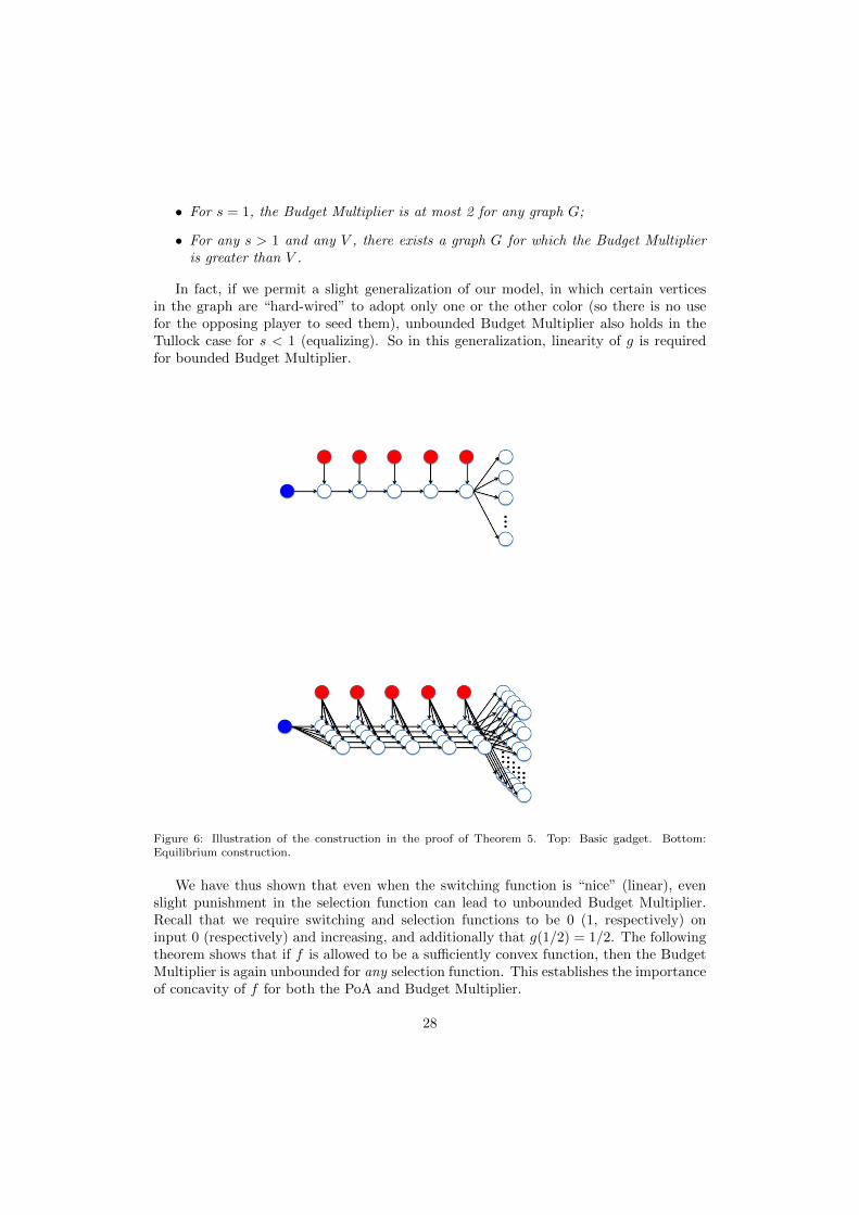
• For s = 1, the Budget Multiplier is at most 2 for any graph G;

• For any s > 1 and any V , there exists a graph G for which the Budget Multiplieris greater than V .

In fact, if we permit a slight generalization of our model, in which certain verticesin the graph are “hard-wired” to adopt only one or the other color (so there is no usefor the opposing player to seed them), unbounded Budget Multiplier also holds in theTullock case for s < 1 (equalizing). So in this generalization, linearity of g is requiredfor bounded Budget Multiplier.

Figure 6: Illustration of the construction in the proof of Theorem 5. Top: Basic gadget. Bottom:Equilibrium construction.

We have thus shown that even when the switching function is “nice” (linear), evenslight punishment in the selection function can lead to unbounded Budget Multiplier.Recall that we require switching and selection functions to be 0 (1, respectively) oninput 0 (respectively) and increasing, and additionally that g(1/2) = 1/2. The followingtheorem shows that if f is allowed to be a sufficiently convex function, then the BudgetMultiplier is again unbounded for any selection function. This establishes the importanceof concavity of f for both the PoA and Budget Multiplier.

28

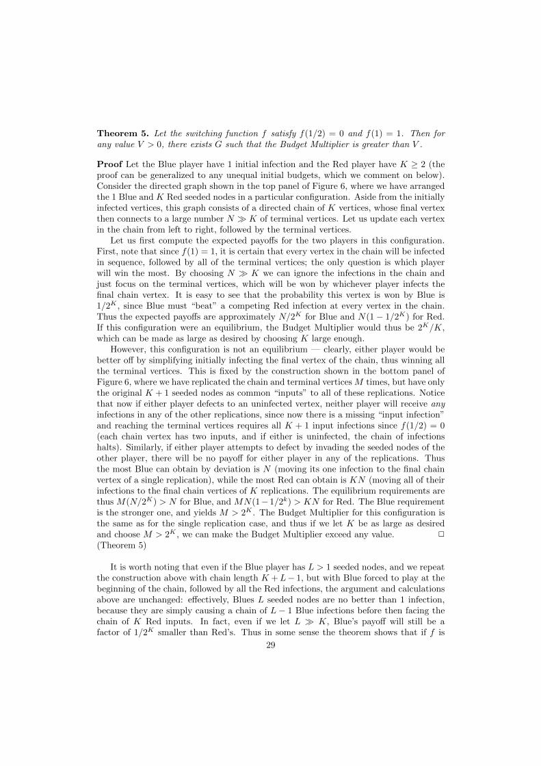
Theorem 5. Let the switching function f satisfy f(1/2) = 0 and f(1) = 1. Then forany value V > 0, there exists G such that the Budget Multiplier is greater than V .

Proof Let the Blue player have 1 initial infection and the Red player have K ≥ 2 (theproof can be generalized to any unequal initial budgets, which we comment on below).Consider the directed graph shown in the top panel of Figure 6, where we have arrangedthe 1 Blue and K Red seeded nodes in a particular configuration. Aside from the initiallyinfected vertices, this graph consists of a directed chain of K vertices, whose final vertexthen connects to a large number N � K of terminal vertices. Let us update each vertexin the chain from left to right, followed by the terminal vertices.

Let us first compute the expected payoffs for the two players in this configuration.First, note that since f(1) = 1, it is certain that every vertex in the chain will be infectedin sequence, followed by all of the terminal vertices; the only question is which playerwill win the most. By choosing N � K we can ignore the infections in the chain andjust focus on the terminal vertices, which will be won by whichever player infects thefinal chain vertex. It is easy to see that the probability this vertex is won by Blue is1/2K , since Blue must “beat” a competing Red infection at every vertex in the chain.Thus the expected payoffs are approximately N/2K for Blue and N(1− 1/2K) for Red.If this configuration were an equilibrium, the Budget Multiplier would thus be 2K/K,which can be made as large as desired by choosing K large enough.

However, this configuration is not an equilibrium — clearly, either player would bebetter off by simplifying initially infecting the final vertex of the chain, thus winning allthe terminal vertices. This is fixed by the construction shown in the bottom panel ofFigure 6, where we have replicated the chain and terminal vertices M times, but have onlythe original K + 1 seeded nodes as common “inputs” to all of these replications. Noticethat now if either player defects to an uninfected vertex, neither player will receive anyinfections in any of the other replications, since now there is a missing “input infection”and reaching the terminal vertices requires all K + 1 input infections since f(1/2) = 0(each chain vertex has two inputs, and if either is uninfected, the chain of infectionshalts). Similarly, if either player attempts to defect by invading the seeded nodes of theother player, there will be no payoff for either player in any of the replications. Thusthe most Blue can obtain by deviation is N (moving its one infection to the final chainvertex of a single replication), while the most Red can obtain is KN (moving all of theirinfections to the final chain vertices of K replications. The equilibrium requirements arethus M(N/2K) > N for Blue, and MN(1−1/2k) > KN for Red. The Blue requirementis the stronger one, and yields M > 2K . The Budget Multiplier for this configuration isthe same as for the single replication case, and thus if we let K be as large as desiredand choose M > 2K , we can make the Budget Multiplier exceed any value. 2

(Theorem 5)

It is worth noting that even if the Blue player has L > 1 seeded nodes, and we repeatthe construction above with chain length K +L− 1, but with Blue forced to play at thebeginning of the chain, followed by all the Red infections, the argument and calculationsabove are unchanged: effectively, Blues L seeded nodes are no better than 1 infection,because they are simply causing a chain of L − 1 Blue infections before then facing thechain of K Red inputs. In fact, even if we let L � K, Blue’s payoff will still be afactor of 1/2K smaller than Red’s. Thus in some sense the theorem shows that if f is

29

sufficiently convex, not only is the Budget Multiplier unbounded, but the much smallerinitial budget may yield arbitrarily higher payoffs!

9. Concluding Remarks

We have developed a general framework for the study of competition between firmswho use their resources to maximize adoption of their product by consumers locatedin a social network. This framework yields a very rich class of competitive strategies,which depend in subtle ways on the dynamics, the relative budgets of the players and thestructure of the social network. We identified properties of the dynamics of local adoptionunder which resource use by players is efficient or unboundedly inefficient. Similarly, weidentified adoption dynamics for which networks neutralize or dramatically accentuateex-ante resource difference across players.

There are a number of other questions which can be fruitfully investigated withinour framework. One obvious direction is to understand the structure of equilibria ingreater detail, and in particular how it is related to network structure. While our resultson the PoA and Budget Multiplier demonstrate that network structure can interact indramatic ways with the switching and selection functions at equilibrium, a more generaland detailed understanding would be of interest.

Other interesting directions include algorithmic issues such as computing equilibriaand best responses in our framework, and how their difficulty depends on the switchingand selection functions; and the multi-stage version of our game, in which the two firmsmay gradually spend their seed budgets in a way that depends on the evolving state ofthe network.

References

[1] J. Coleman, Medical Innovation: A Diffusion Study, 2nd Edition, Bobbs-Merrill, 1966, new York.[2] T. Conley, C. Udry, Learning about a new technology: Pineapple in ghana, American Economic

Review (2010) 35–69.[3] A. Foster, M. Rosenzweig, Learning by doing and learning from others: Human capital and technical

change in agriculture, Journal of Political Economy 103 (6) (1995) 1176–1209.[4] L. Feick, L. Price, The market maven: A diffuser of marketplace information, Journal of Marketing

51 (1) (1987) 83–97.[5] P. Reingen, B. Foster, J. Brown, S. Seidman, Brand congruence in interpersonal relations: A social

network analysis, The Journal of Consumer Research 11 (3) (1984) 771–783.[6] D. Godes, D. Mayzlin, Using online conversations to study word of mouth communication, Market-

ing Science 23 (4) (2004) 545–560.[7] S. Bharathi, D. Kempe, M. Salek, Competitive influence maximization in social networks, Internet

and Network Economics Lecture Notes in Computer Science 4858 (2007) 306–311.[8] A. Borodin, Y. Filmus, J. Oren, Threshold models for competitive influence in social networks,

Proc. Workshop on Internet and Network Economics (WINE) (2010) 539–550.[9] G. Chasparis, J. Shamma, Control of preferences in social networks, 49th IEEE Conference on

Decision and Control (2010) 6651–6656.[10] G. Tullock, Towards a theory of the rent-seeking society, Texas A&M University Press, 1980.[11] S. Skaperdas, Contest success functions, Economic Theory 7 (2) (1996) 283–290.[12] G. Butters, Equilibrium distribution of prices and advertising, Review of Economic Studies 44

(1977) 465–492.[13] G. Grossman, C. Shapiro, Informative advertising with differentiated products, Review of Economic

Studies 51 (1984) 63–82.[14] E. Koutsoupias, C. Papadimitriou, Worst-case equilibria, STACS (1999) 404–413.

30

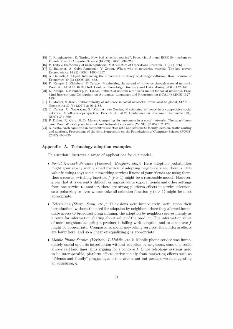
[15] T. Roughgarden, E. Tardos, How bad is selfish routing?, Proc. 41st Annual IEEE Symposium onFoundations of Computer Science (FOCS) (2000) 236–259.

[16] P. Dubey, Inefficiency of nash equilibria, Mathematics of Operations Research 11 (1) (1986) 1–8.[17] C. Ballester, A. Calvo-Armengol, Y. Zenou, Who’s who in networks. wanted: The key player,

Econometrica 74 (5) (2006) 1403–1417.[18] A. Galeotti, S. Goyal, Influencing the influencers: a theory of strategic diffusion, Rand Journal of

Economics 40 (3) (2009) 509–532.[19] D. Kempe, J. Kleinberg, E. Tardos., Maximizing the spread of influence through a social network,

Proc. 9th ACM SIGKDD Intl. Conf. on Knowledge Discovery and Data Mining (2003) 137–146.[20] D. Kempe, J. Kleinberg, E. Tardos, Influential nodesin a diffusion model for social networks, Proc.

32nd International Colloquium on Automata, Languages and Programming (ICALP) (2005) 1127–1138.

[21] E. Mossel, S. Roch, Submodularity of influence in social networks: From local to global, SIAM J.Computing 39 (6) (2007) 2176–2188.

[22] T. Carnes, C. Nagarajan, S. Wild, A. van Zuylen, Maximizing influence in a competitive socialnetwork: A follower’s perspective, Proc. Ninth ACM Conference on Electronic Commerce (EC)(2007) 351–360.

[23] P. Dubey, R. Garg, B. D. Meyer, Competing for customers in a social network: The quasi-linearcase, Proc. Workshop on Internet and Network Economics (WINE) (2006) 162–173.

[24] A. Vetta, Nash equilibria in competitive societies with applications to facility location, traffic routingand auctions, Proceedings of the 43rd Symposium on the Foundations of Computer Science (FOCS)(2002) 416–425.

Appendix A. Technology adoption examples

This section illustrates a range of applications for our model.

• Social Network Services (Facebook, Google+, etc.): Here adoption probabilitiesmight grow slowly with a small fraction of adopting neighbors, since there is littlevalue in using (any) social networking services if none of your friends are using them;thus a convex switching function f (r > 1) might be a reasonable model. However,given that it is currently difficult or impossible to export friends and other settingsfrom one service to another, there are strong platform effects in service selection,so a polarizing or even winner-take-all selection function g (s > 1) might be mostappropriate.

• Televisions (Sharp, Sony, etc.): Televisions were immediately useful upon theirintroduction, without the need for adoption by neighbors, since they allowed imme-diate access to broadcast programming; the adoption by neighbors serves mainly asa route for information sharing about value of the product. The information valueof more neighbors adopting a product is falling with adoption and so a concave fmight be appropriate. Compared to social networking services, the platform effectsare lower here, and so a linear or equalizing g is appropriate.

• Mobile Phone Service (Verizon, T-Mobile, etc.): Mobile phone service was imme-diately useful upon its introduction without adoption by neighbors, since one couldalways call land lines, thus arguing for a concave f . Since telephony systems needto be interoperable, platform effects derive mainly from marketing efforts such as“Friends and Family” programs, and thus are extant but perhaps weak, suggestingan equalizing g.

31

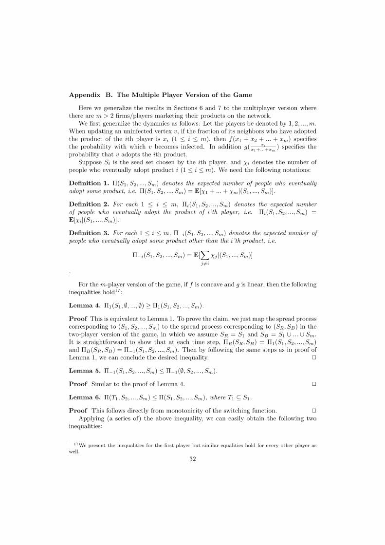
Appendix B. The Multiple Player Version of the Game

Here we generalize the results in Sections 6 and 7 to the multiplayer version wherethere are m > 2 firms/players marketing their products on the network.

We first generalize the dynamics as follows: Let the players be denoted by 1, 2, ...,m.When updating an uninfected vertex v, if the fraction of its neighbors who have adoptedthe product of the ith player is xi (1 ≤ i ≤ m), then f(x1 + x2 + ... + xm) specifiesthe probability with which v becomes infected. In addition g( xi

x1+...+xm) specifies the

probability that v adopts the ith product.Suppose Si is the seed set chosen by the ith player, and χi denotes the number of

people who eventually adopt product i (1 ≤ i ≤ m). We need the following notations:

Definition 1. Π(S1, S2, ..., Sm) denotes the expected number of people who eventuallyadopt some product, i.e. Π(S1, S2, ..., Sm) = E[χ1 + ...+ χm|(S1, ..., Sm)].

Definition 2. For each 1 ≤ i ≤ m, Πi(S1, S2, ..., Sm) denotes the expected numberof people who eventually adopt the product of i’th player, i.e. Πi(S1, S2, ..., Sm) =E[χi|(S1, ..., Sm)].

Definition 3. For each 1 ≤ i ≤ m, Π−i(S1, S2, ..., Sm) denotes the expected number ofpeople who eventually adopt some product other than the i’th product, i.e.

Π−i(S1, S2, ..., Sm) = E[∑j 6=i

χj |(S1, ..., Sm)]

.

For the m-player version of the game, if f is concave and g is linear, then the followinginequalities hold17:

Lemma 4. Π1(S1, ∅, ..., ∅) ≥ Π1(S1, S2, ..., Sm).

Proof This is equivalent to Lemma 1. To prove the claim, we just map the spread processcorresponding to (S1, S2, ..., Sm) to the spread process corresponding to (SR, SB) in thetwo-player version of the game, in which we assume SR = S1 and SB = S1 ∪ ... ∪ Sm.It is straightforward to show that at each time step, ΠR(SR, SB) = Π1(S1, S2, ..., Sm)and ΠB(SR, SB) = Π−1(S1, S2, ..., Sm). Then by following the same steps as in proof ofLemma 1, we can conclude the desired inequality. 2

Lemma 5. Π−1(S1, S2, ..., Sm) ≤ Π−1(∅, S2, ..., Sm).

Proof Similar to the proof of Lemma 4. 2

Lemma 6. Π(T1, S2, ..., Sm) ≤ Π(S1, S2, ..., Sm), where T1 ⊆ S1.

Proof This follows directly from monotonicity of the switching function. 2

Applying (a series of) the above inequality, we can easily obtain the following twoinequalities:

17We present the inequalities for the first player but similar equalities hold for every other player aswell.

32

Corollary 5. Π(S1, S2, ..., Sm) ≥ Π(S1, ∅, ..., ∅).

Corollary 6. Π(S1, S2, ..., Sm) ≥ Π(∅, S2, ..., Sm).

We are now ready to show that for the multiplayer version of the game, there is anO(m) upper bound on the PoA, when the switching function is concave and the selectionfunction is linear:

Theorem 6. When there are m players (m > 2) competing, if f is concave and g islinear, then the PoA is less than or equal to 2m.

Proof Suppose not, and there is a graph G in which PoA is greater than 2m. Let(S1, S2, ..., Sm) denote the strategy profile of players in the worst equilibrium, and(S∗1 , S

∗2 , ..., S

∗m) denote the strategy that maximizes the total number of infections. Since

PoA is greater than 2m, we have:

1

2mΠ(S∗1 , S

∗2 , ..., S

∗m) > Π(S1, S2, ..., Sm) (B.1)

which is equivalent to:

1

mΠ(S∗1 , S

∗2 , ..., S

∗m) > 2Π(S1, S2, ..., Sm) (B.2)

In addition, according to pigeon hole principle, there is a player i such that

Πi(S∗1 , S

∗2 , ..., S

∗m) ≥ 1

mΠ(S∗1 , S

∗2 , ..., S

∗m)

Without loss of generality, assume i = 1 and we have:

Π1(S∗1 , S∗2 , ..., S

∗m) ≥ 1

mΠ(S∗1 , S

∗2 , ..., S

∗m) (B.3)

According to lemma 4:

Π1(S∗1 , ∅, ..., ∅) ≥ Π1(S∗1 , S∗2 , ..., S

∗m) (B.4)

So combining the above with inequality B.3 we have:

Π1(S∗1 , ∅, ..., ∅) ≥1

mΠ(S∗1 , S

∗2 , ..., S

∗m) (B.5)

Now we replace the strategy of the first player in the worst equilibrium, i.e. S1, withS∗1 and show that Π1(S∗1 , S2, ..., Sm) > Π1(S1, S2, ..., Sm). This means that S1 is not thebest response to S−1, which contradicts with the assumption of being in an equilibrium,and it finishes the proof.

We just need to prove that the above inequality holds.According to corollary 5, we have Π(S∗1 , S2, ..., Sm) ≥ Π(S∗1 , ∅, ..., ∅). Combining this

with inequality B.5 we get Π(S∗1 , S2, ..., Sm) ≥ 1mΠ(S∗1 , S

∗2 , ..., S

∗m). Then combining this

last inequality with inequality B.2, we have:

Π(S∗1 , S2, ..., Sm) > 2Π(S1, S2, ..., Sm) (B.6)

33

or equivalently:

1

2Π(S∗1 , S2, ..., Sm) > Π(S1, S2, ..., Sm) (B.7)

On the other hand, according to corollary 6, Π(∅, S2, ..., Sm) < Π(S1, S2, ..., Sm), andtherefore combining with equation B.7 we get:

1

2Π(S∗1 , S2, ..., Sm) > Π(∅, S2, ..., Sm) (B.8)

According to lemma 5, we know that Π−1(S∗1 , S2, ..., Sm) ≤ Π−1(∅, S2, ..., Sm). Basedon the fact that Π(∅, S2, ..., Sm) = Π−1(∅, S2, ..., Sm), we can write it as

Π−1(S∗1 , S2, ..., Sm) ≤ Π(∅, S2, ..., Sm)

Now combining this last inequality with B.8 we get:

1

2Π(S∗1 , S2, ..., Sm) > Π−1(S∗1 , S2, ..., Sm) (B.9)

Since by definition Π(S∗1 , S2, ..., Sm) = Π−1(S∗1 , S2, ..., Sm) + Π1(S∗1 , S2, ..., Sm), andby inequality B.8 we have 1

2Π(S∗1 , S2, ..., Sm) > Π−1(S∗1 , S2, ..., Sm), the following holds:

Π1(S∗1 , S2, ..., Sm) >1

2Π(S∗1 , S2, ..., Sm). (B.10)

According to inequality B.7 we have that Π1(S∗1 , S2, ..., Sm) > Π(S1, S2, ..., Sm).Since it is obvious that Π(S1, S2, ..., Sm) ≥ Π1(S1, S2, ..., Sm), we can conclude thatΠ1(S∗1 , S2, ..., Sm) > Π1(S1, S2, ..., Sm) as desired. 2

It is easy to see that the rest of the results can also be generalized to the multiplayerversion. Since the proofs are straightforward, we just state the results here:

Theorem 7. When there are m players (m > 2) competing, if f is slightly convex andg is linear, then the PoS can be unbounded.

To accommodate the definition of the Budget Multiplier for the case of more than 2players, we change the definition as follows: For any fixed graph, local dynamics, andinitial budgets, with K1 ≥ K2 ≥ ... ≥ Km, let (σ1, σ2, ..., σm) be the Nash equilibriumthat maximizes the quantity

Πi(σ1, σ2, ..., σm)

Πj(σ1, σ2, ..., σm)× Kj

Ki

among all Nash equilibria (σ1, σ2, ..., σm) and and all choices of 1 ≤ i < j ≤ m; Theresulting maximized quantity is the Budget Multiplier.

Theorem 8. When there are m players (m > 2) competing, if f is concave and g islinear, then the pure strategy Budget Multiplier is bounded by 2 across all networks.

Theorem 9. When there are m players (m > 2) competing, if f is slightly convex andg is linear, then the Budget Multiplier can be unbounded.

34