Competition, Regulation and IntegrationIn International Financial Markets

J ens Nystedt

AKADEMISK AVHANDLING

Som for avlaggande av ekonomie doktorsexamenvid Handelshogskolan i Stockholm framlaggs for offentlig

granskning fredagen den3 December 2004, k10ckan 15.15 i sal KAW

Handelshogskolan Sveavagen 65

Competition, Regulation and IntegrationIn International Financial Markets

~~~STOCKHOLMSCHOOL'JJ<l)=U OF ECONOMICS~.~j'~.!1

• HANDELSHGGSKOLAN I STOCKHOLM

EFI, The Economic Research Institute

EFI MissionEFI, the Economic Research Institute at the Stockholnl School of Economics, is a scientificinstitution which works independently of economic, political and sectional interests. It conductstheoretical and empirical research in the Inanagement and economic sciences, including selectedrelated disciplines. The Institute encourages and assists in the publication and distribution of itsresearch findings and is also involved in the doctoral education at the Stockholm School ofEconomics. At EFI, the researchers select their projects based on the need for theoretical orpractical development of a research domain, on methodological interests, and on the generality of aproblem.

Research OrganizationThe research activities at the Institute are organized in 21 Research Centers within eight ResearchAreas. Center Directors are professors at the Stockholm School of Economics.

ORGANIZATION AND MANAGEMENTManagement and Organisation (A)Center for Ethics and Economics (CEE)Center for Entrepreneurship and Business Creation (E)Public Management (F)Infonnation Management (1)Center for People and Organization (PMO)Center for Innovation and Operations Management (T)ECONOMIC PSYCHOLOGYCenter for Risk Research (CFR)Econonlic Psychology (P)MARKETINGCenter for Consumer Marketing (CCM)Center for Information and Communication

Research (CrC)Marketing, Distribution and Industry Dynamics (D)ACCOUNTING, CONTROL AND CORPORATE FINANCEAccounting and Managerial Finance (B)Center for Financial Analysis and Managerial

Econolnics in Accounting (BFAC)FINANCEFinance (FI)ECONOMICSCenter for Health Economics (CRE)International Economics and Geography (lEG)Economic~ (S)ECONOMIC STATISTICSEconomic Statistics (ES)LAWLaw (RV)Center for Tax Law

Prof Sven-Erik SjostrandAdj Prof Hans de GeerProf Carin HolmquistProfNils BrunssonProf Mats LundebergProf Jan LowstedtProf Christer Karlsson

Prof Lelulart SjobergProf Guje Sevon

Acting Prof Magnus Soderlund

Adj Prof Bertil ThorngrenProf Bjom Axelsson

Prof Johnny Lind

Prof Kenth Skogsvik

Prof Clas Bergstrom

Prof Bengt JonssonProf Mats LundahlProf Lars Bergman

Prof Anders Westlund

Prof Erik N erepProf Bertil Wiman

Chair ofthe Board: Professor Carin Holmquist Director: Associate Professor Filip Wijkstrom

AddressEPI, Box 6501, 8E-113 83 Stockholm, Sweden • Homepage: www.hhs.se/efi/Telephone: +46(0)8-736 90 00 • Fax: +46(0)8-31 62 70 • E-mail efi@hhs.se

Competition, Regulation and Integration

In International Financial Markets

Jens Nystedt

:&,j;;-::-~~\ HANDELSHOGSKOLANli~(I)~,

·~~i:1 I STOCKHOLM~.~~."" STOCKHOLM. SCHOOL OF ECONOMICS

EFI, Ekonomiska Forskningsinstitutet

Dissertation for the Degree ofDoctor ofPhilosophy, Ph.D.Stockholm School of Economics 2004

© EFI and the authorISBN nr 91-7258-651-6

KeywordsDerivative Market Competition, OTe Derivatives, Private Sector Involvement, SovereignDebt Restructuring, Default, Equity Market Integration, European Union, EuropeanMonetary Union.

Printed byElanders Gotab, Stockholm 2004

Distributed by:EFI, The Economic Research InstituteStockholm School ofEconomicsPOBox 6501, SE 1-113 83 Stockholm, Swedenwww.hhs.se/efi

To Ana Luisa

Acknowledgements

There are many family, friends, and colleagues to whom I am indebted to for havingmade this thesis a reality.

First and foremost, my wife Ana Luisa who with her love, patience and support never losthope that I could bring this project to a successful conclusion. She sacrificed manyweekends and nights and gave freely of her time in order to free up time for me to write.She bore an unequal burden for a number of years for which I am truly grateful. Finally, Ican carry my share again. Of course, my father Bo and my brother Johan also deserve aspecial mention for having always been there and their willingness to suffer countlesshours discussing esoterics still amazes me. In addition, of course, my sister Jessika foralways believing in me.

Next, Clas Bergstrom, who not only was the one who initially accepted me to the Ph.D.program, but who also stayed in touch me all those years and becan1e a true friend. BothClas and Peter Englund showed remarkable patience and faith in believing in me andwere always ready to assist by giving advice long distance or being there when I did myyearly trip to present my latest progress in one form of another. As with my wife, thisthesis would not have been possible without your help, guidance, and friendship. Also mysincere thanks to my discussant Professor Arnoud Boot, whose visits and seminars at theStockholm School of Economics are one of the main reasons for my interest in the nexusbetween regulation, international economics and finance.

To my colleagues and friends in Sweden, the United States as well as at the StockholmSchool of Economics and the International Monetary Fund I remain in deep gratitude.You certainly helped me finish this journey and kept my spirits up, my focus on the goal,and provided support when I asked. While there are many of you, there are a few I wantto mention especially:

Gustaf, Johan, Staffan, Magnus, Joel, and Patrick, my officemates and fellow studentsduring our Ph.D. studies at the SSE. Your companionship was invaluable and certainlybroke the boredom of studying too hard, getting stuck, or correcting too many examsduring our courses.Hc1kan and Peter, who both remained by my side regardless of wherever next I happenedto move. I hope that my experience at least to some extent convinced Hakan that pursuinga Ph.D. is definitely worthwhile.Binky, Maziar, and Miguel. All three of them started of as colleagues, but grew into truefriends. Whether you know it or not at different points in time your encouragement wascritical in helping me push that one last bit.

Finally, I would like to thank the Tore Browaldh foundation for their financial supportduring the early stages of this thesis.

Introduction and Abstracts

Chapter I - Derivative Market Competition: OTC Markets VersusOrganized Derivative Exchanges

I. Introduction 1

II. Literature Overview 5

III. The Model 6A. Basic Design 7B. The Markets' Maximization Problems 11

IV. Comparative Statics and Model Results 21A. Comparative Statics 22B. Additional Model Results 24

V. Analysis and Policy Implications 26

VI. Conclusions 27

Appendix1. Numerical Example 292. Regulatory and Supervisory Treatment ofOTC Versus ODE Derivative in

the United States 37

References 41

Chapter II - Crisis Resolution and Private Sector Adaptation

I. Introduction 43

II. Relevant Literature 46

III. Determinants ofDebt Restructuring: A Model 50A. The Sovereign Debtor 50B. The Creditor 52C. The Equilibrium Coupon 52D. Cost of Default and the Equlibrium Coupon 53E. Probability ofPayment and Recovery Value 55F. Effect on Secondary Market Price ofAlready Exisiting Debt. 56G. Implications 57

IV. Extending the Model: Private Sector Adaptation 58A. Model Extension 58B. Numerical Example 60

V. Debt Payment Suspensions: Private Sector Reaction and Adaptation 61A. Issues Regarding Orderly Payment Suspensions 63B. Payment Suspensions and the Composition of Cross-Border Debt Flows 65C. Implications 66

VI. Bond Exchanges and Private Sector Adaptation 67A. Impact on Outstanding Bonds and Bond Restructurings 68B. Cost of Default, Legal Innovations and the Threat of Litigation 70C. Changing the Structure of the Eurobond Market. 72

VII. Implications and Conclusions 73

Appendix1. Overview of the Ecuador Bond Exchange 752. Innovations in the Ecuador Bond Exchange 773. Background on Elliott Associates versus Peru 78

References 80

Chapter III - European Equity Market Integration: Cyclical or Structural?

I. Introduction 83

II. Financial Market Integration in the Literature 85

III. Euroland and International Institutional Investors 88

IV. Data 92

V. Average Sector and Country Correlations 93

VI. Time-Varying Sector and Country Sensitivities 97

VII. Robustness of Results and Impact of the Euro? 102

VIII. Summary and Conclusions 104

Appendix1. Key Tables and Figures 1062. Biases ofAlternative Approaches 112

References 114

Introduction and Abstracts

Chapter I - Derivative Market Competition: OTC Markets VersusOrganized Derivative Exchanges

Recent regulatory initiatives in the United States have again raised the issue of a "levelregulatory and supervisory playing field" and the degree of competition globally betweenover-the-counter (OTC) derivatives and organized derivative exchange (ODE) markets.This chapter models sonle important aspects ofhow an ODE market interrelates with theOTC markets. It analyzes various ways in which an ODE market can respond tocompetition from the aTe markets and considers whether ODE markets would actuallybenefit from a more level playing field. Among other factors, such as different transactioncosts, different abilities to mitigate credit risk playa significant role in determining thedegree of competition between the~two types ofmarkets. This implies that a potentiallyimportant service ODE markets can provide aTC market participants is to extendclearing services to them. Such services would allow the OTC markets to focus more onproviding less competitive contracts/innovations and instead customize their contracts tospecific investors' risk preferences and needs.

Chapter II - Crisis Resolution and Private Sector Adaptation

Efforts at crisis resolution that succeed in reducing potential inefficiencies and instabilityin the international financial system are in the interest ofboth the private and the publicsector. Unlike in the domestic context, in the international context, in the absence ofclearly established rules of the game, the approaches adopted toward crisis resolution, andthe extent to which they are interpreted by market participants as setting a precedent, canhave profound implications for the nature and structure of international capital flows. Thekey conclusion of this chapter is that recent experiences with payment suspensions andbond restructurings are limited as guides to determining the future success or failures ofthese initiatives, as the private sector most likely has adapted in order to minimize anyunwanted public sector involvement.

Chapter III - European Equity Market Integration: Cyclical or Structural?

Reviewing the empirical evidence of equity market integration in the European Union,the chapter finds a significant increase in the inlportance of global sector factors for anumber of industries. Unlike most past studies, which only covered developments duringthe bull market of the late nineties, the results presented in this chapter suggest that thedegree of Euroland equity market integration has declined gradually following thebursting of the TMT bubble. This seems to suggest that the findings ofprevious studiesthat Euroland equity markets were nearly fully financially integrated is worth revisiting.There are, however, several good reasons to believe that the structural factors drivingEuropean equity market integration have yet to play themselves out fully. Institutionalinvestors both outside the Euroland area and within have substantial untapped capacity totake on Euroland exposures and invest additionally in Euroland equities.

1

Chapter IDerivative Market Competition: OTC Markets Versus

Organized Derivative Exchanges}

I. INTRODUCTION

".. This is a critical time for all us. futures exchanges. Our continued viability is beingseriously threatened by two sources ofcompetition-over-the-counter derivatives andforeign futures exchanges. ,,2

"..It is no secret that the combined onslaught ofglobalization, Over-the-Counter (OTC)competition, and technological advancement, have put enormous pressure on traditionalfutures exchanges. Indeed in some quarters, there is a growing beliefthat the good daysfor traditional exchanges is behind them. ,,3

The recent global surge in the use ofvarious fonns of financial derivatives utilizing arange of different markets and counterparties highlights the importance of furtherunderstanding how different types of derivative markets compete with and complementeach other. This understanding is vital as most of the recent spectacular growth has takenplace through an increase in the use of OTe derivatives (over-the-counter, lightlysupervised and self-regulated derivatives.)4 Many organized derivatives exchange markets(liquid, supervised, and regulated) have argued that they are at a comparativedisadvantage to OTe derivatives markets, highlighting, in particular, the lack of a levelplaying field as the regulatory and supervisory regimes differ. From a supervisor's

1 The author wishes to thank Clas Bergstroem, Bankim Chadha, Peter Englund, ToddSnlith, Matthew Spiegel, Staffan Viotti, an anonymous referee, and seminar participantsat the International Monetary Fund and the Stockholm School ofEconomics for helpfulcomments. Any remaining errors are those of the author.

2 Patrick H. Arbor, the fonner ChaiIman of the Chicago Board of Trade (CBOT).Quotation taken from his testimony before the Risk Management and Specialty CropsSubcommittee of the (U.S.) House Agriculture Committee, April 15, 1997.

3 Speech delivered at the 2000 Canadian Annual Derivatives Conference by LeoMelamed, chairman emeritus of: and senior policy advisor to, the Chicago MercantileExchange.

4aTe markets are by no means unregulated, but rather self-regulated. Industryassociations such as International Swaps and Derivative Association (ISDA) provide theaTC markets with standard legal contracts for most types of instruments. This paperassumes, not unreasonably, that this self-regulation gives the aTe market a significantcost advantage over organized exchange markets. For more infonnation, seewww.isda.org.

2

perspective the trend toward the increased use of aTC derivatives, potentially at theexpense of exchange-traded derivatives, raises systemic risk issues given theconcentration of aTC derivatives among a few market participants and their lack oftransparency. Following a string of crises related to the use of aTC derivatives (mostrecently involving Enron, but previously Long-Term Capital Management,Metallgesellschaft, etc.), recent discussion among supervisors has focused increasingly onwhether aTC derivatives should be more closely supervised, regulated, and whetherinvestors need to set aside more capital when trading aTC. This chapter analyzes severalaspects of the interrelationship between the organized derivatives exchange markets andthe aTe derivatives markets, and the degree to which the different markets' microstructure impacts on their operation. It will also address the issue ofwhether organizedderivatives exchange nlarkets actually stand to gain from reducing the OTe market's riskaversion through various vehicles, including insisting on a level regulatory playing filed.

In contrast to the highly standardized (and generally cleared) contracts offered bytraditional organized derivatives exchange markets (ODEs), OTC derivatives can beindividually customized to an end-user's risk preference and tolerance (see Schinasi andothers (2000)). Although nearly two-thirds of the actual aTC derivatives traded are of afairly sin1ple contract structure (for example, a fixed for floating interest rate swap), theirterms are still individually determined and highly flexible. One leading industry groupdefines OTC derivatives as contracts that are"executed outside of the regulated exchangeenvironment whose values depends on (or derives from) the value of an underlying asset,reference rate or index." 5 6 Clearly, the difference between an aDE derivative and anaTC derivative may involve not only where they are traded but also how. In the UnitedStates much attention has centered on pure OTC derivatives that are privately negotiatedbetween large institutional investors and broker/dealer banks. To minimize definitionalproblems, this chapter will focus on some characterized extremes (see Table 1 fordefinitions).

Table 1. Definition ofDifferent Derivative Markets

Standardized

Cleared, regulated ODE markets, such as, CBOE,CBOT, and Eurex.

Not cleared, self-regulated International Currency and Swapmarket

Not Standardized

Tailor-made clearing

Pure aTe derivatives

The heightened importance of the aTe derivatives markets has been a fairly recentphenomenon. By the end of2001, the size of the global aTC market derivatives was by

5 Group of Thirty (1993). The Group of Thirty is a group established in 1978, which is aprivate, nonprofit, international body composed of very senior representatives of theprivate and public sectors and academia.

6 CFTC (1998).

3

any measurement huge and growing rapidly (see Figure 1 and BIS (2002)).7 Since thefirst triennial survey was completed by the Bank for International Settlement (BIS) in1995, the notional amount ofOTC derivatives outstanding (adjusted for double counting)has increased by more than 130 percent, and by the end of2001 the global amountexceeded US$11 0 trillion. 8 Presently, most aTe derivatives are either related to interestrates (70 percent) or foreign exchange (15 percent). Other types ofaTe derivativeslinked to equities or commodities account for less than 3 percent. While the notionalvalue of aTC derivatives outstanding is significant, their gross market value or"replacement" value, that is, what the derivatives would be worth if they were n1arked tomarket, has increased far less and ranges between 3 and 5 percent of the notional value.Nonetheless, this implies that the market value of all aTe derivatives reached US$3.8trillion by the end of2001.

Figure 1. Evolution of Global Derivatives Market(In US$ billion)

120,000 ._-------_..._-------_. 4,000

3,800

100.000

80.000

--e--Organized Derivative Exchanges - Notional

--OTC Derivatives - Notional......... OTC Derivatives - Gross Market Value (right scale)

3,600

3,400

60,000

40,000 ~.. ,

.A

3,200

3,000

2,800

2,600

20,000 ....2,400

2,200

Dec-DODec-99Dec-98Dec-97Dec-96Dec-95

+-------r----~--__,c__--___r_---,__--___,_---_,...L2,000

Dec-01Dec-94

While the outstanding notional value of aTe derivatives grew, the corresponding use ofODE derivatives remained predominantly flat at US$14 trillion. However, aggressivemonetary policy easing by the U.S. Federal Reserve in 2001, triggered a wave of renewed

7 The economic importance of the global derivatives market can not be overstated. As acomparison, as noted in Schinasi and others (2000), world GDP reached U8$31 trillionand global net capital flows totaled US$394 billion in 1999.

8 See BIS (2002). The notional value of the aTe derivatives outstanding has beenadjusted for double counting and other well-known measurement problems.

4

hedge demand by many market participants leading to sharp increases in the use of bothODE and OTC derivatives. By the end of2001, the share of ODE derivatives in the totalamount of derivatives outstanding reached 17 percent. To a certain extent, the limitedgrowth in the notional value of ODE derivatives masks substantial competition betweendifferent ODE markets. By now famous examples include the rise of the EUREX market(see Schinasi and others (2000)) at the expense of the LIFFE regarding the trading offutures on German treasury bonds.

ODE contracts can generally be split into two main groups in tenns of the notional valueoutstanding: 90 percent are interest rate derivatives and 9.8 percent are linked to equities.Around 60 percent of these derivatives are traded in the form of options while theremainder involves futures. Moreover, as pointed out by Cuny (1995), even ODE marketshave been highly innovative in launching new contracts that are more highly customizedto their end users' needs. While perhaps only a quarter of the new contracts "succeed,"innovation continues to be an important strategy to counter the growth in the use of OTCderivatives. Of course, another strategy is to enhance the ODE market's experience andcomparative advantage with respect to the clearing of transactions, thereby assisting aTemarkets in mitigating counterparty credit risk. From a regulator's perspective, theincreased clearing ofaTe derivatives could help address the problems associated withthe concentration of credit risk among the handful of large international banks that areinvolved in the vast majority ofOTC transactions.9

OTe and ODE derivatives markets can both complement and compete with each other.For instance, the major broker/dealers of OTe derivatives frequently rely on a liquidODE market to dynamically hedge their market risk. Conversely, organized futures andderivatives markets in the U.S. face competitive pressure from OTe markets, which areoffering fairly similar contracts but are unburdened by regulatory and supervisoryoversight. To a certain extent, competition between aTe derivatives and ODE derivativesis determined by the structure of the contracts and the types of risk the end users need tohedge. Hence, it may be useful to analyze how ODE markets can increase theircomparative advantage in highly standardized and liquid derivatives while also providingclearing services for aTe derivatives.

In trying to analyze how ODE markets can respond to the threat posed by aTederivatives, more research is needed to model the interrelationship between thesemarkets. While it is a potentially relevant area for future regulation initiatives, very littleresearch has so far been done on this topic. lo Rather, the main focus of the security designliterature has been on competition between different stock exchanges or ODE markets.This chapter takes a first step in analyzing inter-derivative market competition in amultiple contract setting and draws some policy conclusions regarding how competition

9 For the second quarter of2002, seven commercial banks accounted for 96 percent of thetotal notional amount of derivatives held by the U.S. banking system (estimated atUS$50 trillion; see OCC, 2002). aTe derivatives accounted for 90 percent of the total,and the renlainder was in the form of ODE contracts.

10 An exception is Kroszner (1999).

5

affects the contracts issued by the two markets, their transaction costs, and whether or notODE markets would benefit from reducing OTC market risk aversion and investors'counterparty risk concerns while trading OTC. The main findings of this chapter are thatthe two derivative markets can co-exist in equilibrium while exploiting their comparativeadvantages. Interestingly, the most useful approach for ODE markets to deal with thecompetitive threat posed by OTC markets is to lower transaction costs, target highvariance risks that remain to be hedged, and introduce mechanisms that can help reducethe counterparty credit risk exposure the OTe market faces. This could be achieved, forexample, by providing customized clearing services, which would allow the OTC nlarketto better target those investors with particular types ofrisks.

The remainder of this chapter is structured in the following manner. First, a briefoverview of the literature is provided. Section III is devoted to the model and begins withderiving the chapter's theoretical framework on the basis of the previous security designliterature. In the model provided, the ODE market can launch only one contract, while theOTe market can launch as many as it wishes. A key contribution involves extending therelatively straightforward innovation modeling framework for the ODE market to amarket with a different structure. Sections lILA and III.B then apply the model for eachmarket's optimal contract and transaction cost, and analyze the respective inlpact ontrading volume, competition, and risk diversification are analyzed in the second section (anumerical example is provided in the appendix). This section also discusses the degree towhich the model takes into account credit risk related costs for the investors and the aTemarket, and the effect of this credit risk on market competition. After a discussion of theconlparative statics of the model in Section IV, Section V discusses some potential policylessons that could be drawn. The chapter ends with some conclusions and proposes someavenues for further research. The first appendix discusses some of the model results in thecontext ofvarious numerical examples, while the second appendix analyzes the UnitedStates as an example for some of the regulatory and supervisory challenges facing OTCderivatives compared to ODE derivatives.

II. LITERATURE OVERVIEW

Duffie and Jackson (1989) introduced a useful modeling framework to address issues ofoptimal financial innovations and transaction costs in an incomplete market setting. Inthis strand of the literature, an innovation is defined as the best additional contract givenprevious contracts. This contract/innovation/derivative is optimal ifit spans the largestpossible section of a previously unspanned portion of the incomplete market. In reality,however, markets will always be incomplete, due to the risks that can never be hedged bya financial instrument. The original model by Duffie and Jackson has been extended in atleast two main directions. Tashjian and Weissman (1995) used the approach to analyze afutures exchange that can launch several contracts and how it affected trading volumes.Clearly, the futures market will always design the next new contract in such a way that itis likely to generate the highest additional revenue for the exchange, i.e., it will targetthose investors that have the highest unfilled demand for hedges weighed by their riskaversions. Cuny (1995) enhanced the original model by taking into account the role ofliquidity in the design of the optimal contract and the effect of competition betweenmultiple exchanges over time. These extensions have been further generalized in a varietyofpapers as discussed by the useful surveys completed by Duffie (1992) and Duffie andRam (1995).

6

More recent approaches analyzing multiple exchange competition have brought a varietyof different modeling frameworks to the concepts of innovations, competition, etc. Santosand Sheinkman (2001), for example, ask whether competition between organizedexchanges lead to excessively low standards in terms of the guarantees/collateral tradershave to provide to transact. The authors argue that it has been claimed that the nature ofmarket competition triggers a race for the bottom to maximize trading volun1e byrequiring few performance guarantees/collateral. However, Santos and Sheinkman show,in the context of a two period model (which allows for default among traders but not forthem to trade in multiple markets) that the use of guarantees/collateral is indeedconstrained efficient in a con1petitive setting. Interestingly a monopolistic exchangewould design its securities and guarantees in such a way that actually less collateral isprovided than in a competitive setting. Moreover, the authors argue that the race to thebottom argument is not borne out in empirical research and that the experience with self­regulation is pretty robust with the exception for potentially extreme events (for example,the 1987 stock market crash).

Rahi and Zigrand (2004) analyzes the issue ofmarket competition and financialinnovation from the point ofview of arbitrageurs/speculators. Rather than assuming, as iscommon in the literature, that exchanges design the innovations/contracts, Rahi andZigrand argue that profit seeking agents that trade on the exchanges play an importantrole in the ultimate design of a financial contract. For example, an arbitrageur/speculatoris not only interested in potentially hedging some random endowment but also to identifymispricings or provide liquidity and generate trading profits. Thesearbitrageurs/speculators differ from the typical investor by their ability to trade acrossn1ultiple exchanges. The authors assume that investors predominantly interested inhedging their endowments are limited to their "local" exchange. The resulting securitydesign game is driven by the arbitrageurs in terms ofwhat assets are available for trading.Hence, the model developed in their paper derives an endogenously incomplete set offinancial assets in the context of segmented markets. What is of particular interest is thatRahi and Zigrand's model explains why many of the financial innovations actually seenin the real world are in many times redundant, i.e., they could have been created through acombination ofpreviously existing assets. This result predominantly reflects the rolearbitrageurs/speculators play across markets and their focus on trading profits rather thanmaximizing trading volume and the socially optimal level ofhedge.

The more recent approaches have, as discussed above, shed more light on the variousaspects on who is responsible for launching the innovation, and whether or not marketcon1petition could have potentially less attractive side effects. This chapter takes thecompetition dimension in a new direction by analyzing how two different types ofderivative exchanges compete and what are some of the tentative policy lessons that canbe concluded from some of the n1odel's implications.

III. THE MODEL

The model developed in this chapter will base itself mostly on the Tashjian andWeissman two-period model. New contracts will be of a very stylized form and a zerointerest rate is assumed. While the ODE market is limited to one contract and acts as anintermediary for transactions, the aTe market can issue as many customized contracts as

7

needed as long as it is willing to take the offsetting position to that of the agent. In theoriginal security design literature, short sales presented a problem (see Allen and Gale(1994)), since it allowed all agents to replicate a potentially new contract without costs.The model developed here has no short sale restriction for either the ODE contract or thecustomized OTC contracts. Short sales are allowed as long as all the trading takes placethrough one of the markets. An important difference between the ODE and OTe marketis, however, that the OTC market will hold positions of its own.

In game theoretic terms, the model developed represents a game between a single ODElllarket and a single OTC market. Both markets will sinlultaneously offer contracts to agroup of agents/investors. Risk averse investors (hedgers and speculators depending ontheir initial risky endowments and risk tolerances) will buy or sell a contract dependingon how attractive the contract is. The key difference between the two different contractsis that the OTC contract can be customized to various degrees to hedge an investor'sidiosyncratic risk, something the standardized ODE contract cannot do. At the subsequenttime period the risky payoffs are realized and the game ends. Note that it is not a zerosum game, but there is a maximum volume that can be traded because the nUITlber ofagents in the economy and their endowments are finite. The pareto optimal equilibrium isreached by choosing a set of contracts that maximizes transaction volume and hence theamount of risk transferred. However, non-zero transaction costs, the OTC market's riskaversion, the agents' credit risk aversion, and the less than perfect competition betweenthe two markets will ensure that global trading volume is less than pareto optimal. Onlytwo markets are analyzed, making the resulting game fairly simple and tractable. Treatingthe OTC market as a single concentrated marketplace, which makes the decision ofwhatcontract to launch at what price is another simplifying assunlption. In reality OTCmarkets (see Schinasi and others, 2000, for a detailed description) are more of a looseglobal network of large banks, where the vast majority of transactions are conductedbetween a handful of large participants.

A. Basic Design

The construction of the basic version of the model will begin with the derivation of theagents' optimal demands for the different markets' contracts. Knowing these demands,they can then be aggregated across all the agents in the economy. These aggregateddemands are the central variables in the markets' maximization problems. The motivationfor customization being the key difference between the two markets is that OTe marketparticipants generally view the ability to off-load highly idiosyncratic risks as one of thekey advantages of going to the OTC market. 11 Moreover, small and medium investorswith other transactional motives play, even on the ODE markets, a very small role. 12

11 Which is indeed the most frequently cited reason to use the OTC markets, the OCCattributes the rapid growth in OTC derivatives to "banks clients' increasing use ofcustomized solutions for risk management problems" (OCC, 1999).

12 They reportedly constitute about 4 percent of volume traded on NYSE. Theirinsignificant presence is also valid on the major derivative exchanges (not agriculturalcommodities though).

8

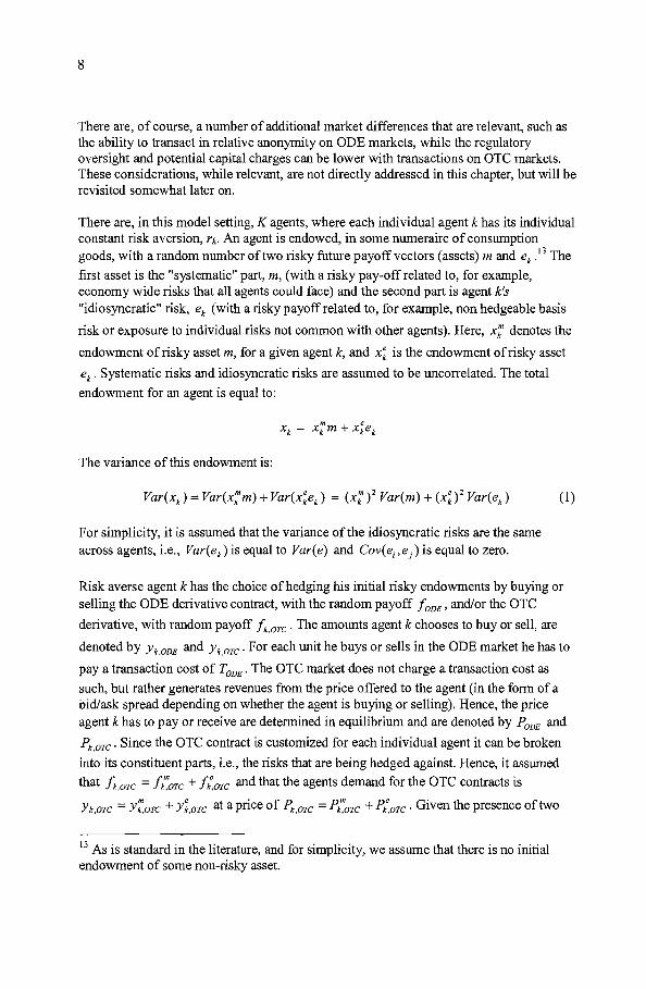
There are, of course, a number of additional market differences that are relevant, such asthe ability to transact in relative anonymity on ODE markets, while the regulatoryoversight and potential capital charges can be lower with transactions on aTe markets.These considerations, while relevant, are not directly addressed in this chapter, but will berevisited somewhat later on.

There are, in this model setting, K agents, where each individual agent k has its individualconstant risk aversion, rk. An agent is endowed, in some numeraire of consumptiongoods, with a random number of two risky future payoff vectors (assets) m and ek .13 The

first asset is the "systematic" part, m, (with a risky pay-off related to, for example,economy wide risks that all agents could face) and the second part is agent k's"idiosyncratic" risk, ek (with a risky payoff related to, for example, non hedgeable basis

risk or exposure to individual risks not common with other agents). Here, x; denotes the

endowment of risky asset m, for a given agent k, and x; is the endowment of risky asset

e/c. Systematic risks and idiosyncratic risks are assumed to be uncorrelated. The total

endownlent for an agent is equal to:

The variance of this endowment is:

For simplicity, it is assumed that the variance of the idiosyncratic risks are the sameacross agents, i.e., Var(ek ) is equal to Var(e) and Cov(ei'e j ) is equal to zero.

Risk averse agent k has the choice of hedging his initial risky endowments by buying orselling the ODE derivative contract, with the random payoff fODE' and/or the aTe

derivative, with random payoff fk,OTC • The amolmts agent k chooses to buy or sell, are

denoted by Yk,ODE and Yk,OTC. For each unit he buys or sells in the aDE market he has to

pay a transaction cost of rODE. The aTe market does not charge a transaction cost as

such, but rather generates revenues from the price offered to the agent (in the form of abid/ask spread depending on whether the agent is buying or selling). Hence, the priceagent k has to payor receive are determined in equilibrium and are denoted by PODE and

Pk,OTC • Since the aTe contract is customized for each individual agent it can be broken

into its constituent parts, i.e., the risks that are being hedged against. Hence, it assumed

that fk,OTC =fk~OTC + fk~OTC and that the agents demand for the aTe contracts is

Yk,OTC = Y~OTC + yZ,OTC at a price of Pk,OTC = Pk~OTC + Pk~OTC. Given the presence of two

13 As is standard in the literature, and for simplicity, we assunle that there is no initialendowment of some non-risky asset.

9

financial markets, agent k is maximizing his utility by maximizing the next periods'payoff taking into account his risk aversion in the fonn of a mean variance type utilityfunction subject to some individual level of risk aversion and with normally distributedpayoffs. 14 To capture an in1portant difference between OTC markets and ODE marketsand the fact that transactions in the ODE market are cleared, agents that transact in theOTC market face additional credit risk aversion Ck for the exposure they face towards the

OTC counterparty

Agent k's maximization function is hence constructed by substituting k's pay-offfunction, i.e., wk ' into the utility function.

Plugging (2) into the agent's mean-variance utility expression, the optin1al demand ofeach contract will depend on how well the contract's payoffhedges k's risky endowments,which is detem1ined by the contract's covariances. In the case of the ODE market, itscontract can, by assumption, only hedge the systematic risk, which means that:

After some derivation, the optimal volume bought or sold by a certain agent k in marketODE is equal to: 15

= 1 [-2rkCOV(X~nm,foDE) - 2r/CY;::OTC COV(!ODE,f;~c)]Yk,ODE 2rkVar(!ODE) + EC!ODE)-PODE + ak,ODETODE (3)

Similarly, the amount bought and sold of the aTe contract addressing m-risk can beexpressed by the below expression:

14 Maximizing a standard mean variance utility function with normally distributed pay­offs is equivalent to maximizing a negative exponential utility function exhibitingconstant absolute risk aversion.

15 The derivation of the individual's optimal volume is relatively straightforward andmore details are provided by Tashjian and Weissman (1995) or Duffie and Jackson(1989). As is standard in the literature, no specific budget constraint is assumed in periodoand agents do not default on their future payment. For a relaxation of the latterassumption please see Santos and Scheinkrnan (2001).

10

m = 1 [- 2rk Cov(x;m, /o~c) - 2rk Yk,oDE CoV(/ODE , !:;TC)]

Y k,OTC 2( )T/ (I'm) ( I'm mrk +Ck yar JOTC + E JOTC)-POTC

(4)While the demand for OTC contract hedging an individual's idiosyncratic risk can beshown to equal:

Y e _ 1 [_ 2r Cov(xee I'e ) + E( I'e ) _ p,e ]k,OTC - 2( )T7 (I'e) k k k' J k,OTC J k,OTC k,OTC (5)rk + ck yar J k,OTC ,

The optimal demand expressions in (3), (4), and (5) show that an agent's demand to buyand sell the ODE and the OTC contracts depends on the variances of the contracts'payoffs, the covariances of the agent's risky endowments with the respective contracts,and the covariances between the contracts. Moreover, the risk aversion of the agent to risk,in general, and GTC-risk, in particular, the expected return of the contracts, and the priceof the contracts also playa role. Of course, the higher the transaction cost of the ODEcontract the less it will be in demand.

Further analyzing (3) the first two terms in the main bracket are referred to as the"hedging component", and the last two tern1S are referred to as the "speculativecomponent" (based on Tashjian and Weissman, 1995). The first term of the "hedgingcomponent" has the effect ofwhether an individual agent tends to have a positive ornegative demand for the contract, if the contract is positively correlated with the agent'spositive endowment he tends to have a negative demand (i.e., supply). The second"hedging" term captures the effect of con1petition with the aTe contract hedging m-risk.The more the two competing contracts are correlated, and if the agent has already hedgedsome ofhis risk using the other contract, his absolute demand for the other contract isless. In the case of the ODE market, the premium/discount (E(foDE) - PODE ) in the third

term relates to how the equilibrium price of the contract encourages "speculators" toprovide additional demand or supply to clear the market (i.e., to ensure that the net supplyin equilibrium is zero). For example, in some cases there might be an imbalance betweenthe agents interested in selling the ODE contract and the agents interested in buying it. Inthose cases the premium has to be increased to induce an increased supply from agentswith a low risk aversion, which allows them to take on additional risk by supplying thecontract and to be compensated for it by the premium. The agents that provide thisadditional supply in the ODE market (or demand if the imbalance is reversed) can beinterpreted as "speculators." Finally the last term in equation (3) captures the effect oftransaction costs on agents' willingness to transact in the ODE market's contract. If agentkhas a negative risky endowment, he is likely to go long in the ODE contract. As a resultak,ODE is equal to -1 and the transaction cost has a negative effect on the k's final demand

for the contract.

Turning to the aTe market, the role of the speculator is being played by the OTC marketitself. Hence, since the counterpart is always the aTe n1arket, that market will set theprice that optimizes the market's return for each individual agent. However, its pricing

11

power in the case ofm-risk is limited by the competition effect provided by the ODEmarket, and the agents' counterparty credit risk aversion.

B. The Markets' Maximization Problems

The two markets are assumed to be interested in maximizing their risk-adjusted revenue.In the case of the ODE market the risk-adjusted revenue is simply the absolute volumetraded in the chosen contract times the chosen transaction cost, since this market does nottake positions of its own. In the case of the aTe market, revenue is generated by thepremium/discount charged by the market times the number ofcontracts adjusted for theriskiness ofthe net position incurred by the aTC market. Each market can, of course,choose the structure of the contract it offers and, when relevant, the transaction cost orprice associated with it. Any contract's structure is defined by the contract's pay-off.

The ODE Market's Maximization Problem

Following the definitions in (3), the optimal individual demand for each contract isaggregated across all agents to derive the total volume traded in the aDE market.Multiplying this volume with the transaction cost per trade results in the revenuemaximization expression for the ODE market.

(6)

How much the competition affects the revenue of the ODE market depends on how muchthe participating agents in the ODE market also trade in the aTC market. The modelallows for agents to transact in both contracts simultaneously. It is clear that the totalvolume traded in each market will be a function ofhow good that market's launchedcontract is at fulfilling the agents' needs and at what costs. The total volume traded in theODE market is defined as:

L.Yk,ODEkeLODE

(7)

The volume expression states that the amount traded in the ODE contract is equal to twotimes the volume bought by the agents going long on the contract. 16 When aggregatingthe agents' optimal demands, see equation (3), over all the agents, and knowing that thenet volume traded is equal to zero, the equilibrium price PODE can be solved:

- 2 L. x;Cov(m, fODE )1 keK

PODE =E(foDE ) +~ (8)LJl/ rk - 2L.Y~oTcCov(fk~OTC ,foDE)+ TODE L. ak,ODEkeK keK keK rk

16 Demand equals supply in equilibrium so the total transaction volume is equal to twotimes the denland.

12

Substituting PODE into the volunle equation by those buying the ODE contract, i.e.,

into LYk,ODE (where LODE represents the agents going long the ODE contract), andkeLODE

using equation (7) the gross volume traded in the ODE contract can be derived as:

VODE = [ 1 keLODE

1 keSO]>JJE

L + L Var(foDE)keLoo~ / rk kesoD~ / rk

[kfo:; k~:;]C ( I' ) T"'" ~ ov m'}ODE - ODE-LJl/ rk LJl/ rk

keSODE keLODE

[~~ - ~~ r

k]COV(fk~OTC ,foDE )

keSODE rk

keLoDE

(9)

Following Tashjian and Weissman's (1995) approach and notation, equation (9) can besubstantially simplified using the definitions presented in Table 2.

Table 2. Definition ofKey Constants

Symbol

rf

rJ

w~J

w~J

Definition

L~keLj rk

L~keSj rk

Explanation

Aggregated risk tolerance for agents going long (L) in marketj.

Aggregated risk tolerance for agents going short (S) in marketj.

Aggregated endowments for agents going long (L) in market j.

Aggregated endowments for agents doing short (8) in market j.

Hence, the equilibrium ODE contract price, equation (8), and the ODE trading volume,equation (9), can be rewritten as:

PODE = E{fODE) + S 1 L (-2(W~DE +w~DE)Var(m)-2v;;;;etVar(m)+(yS -yL)ToDE )r +r

(10)

2 L SV == r ODErODE

ODE (r~DE + r~DE)Var(foDE)

( W~DE W~DE J-s L- Cov(m'!ODE)-ToDE +rODE rODE

(V;TC VtTC J m-s- - -L- Cov(fk,oTc, fODE)rODE rODE

(11)

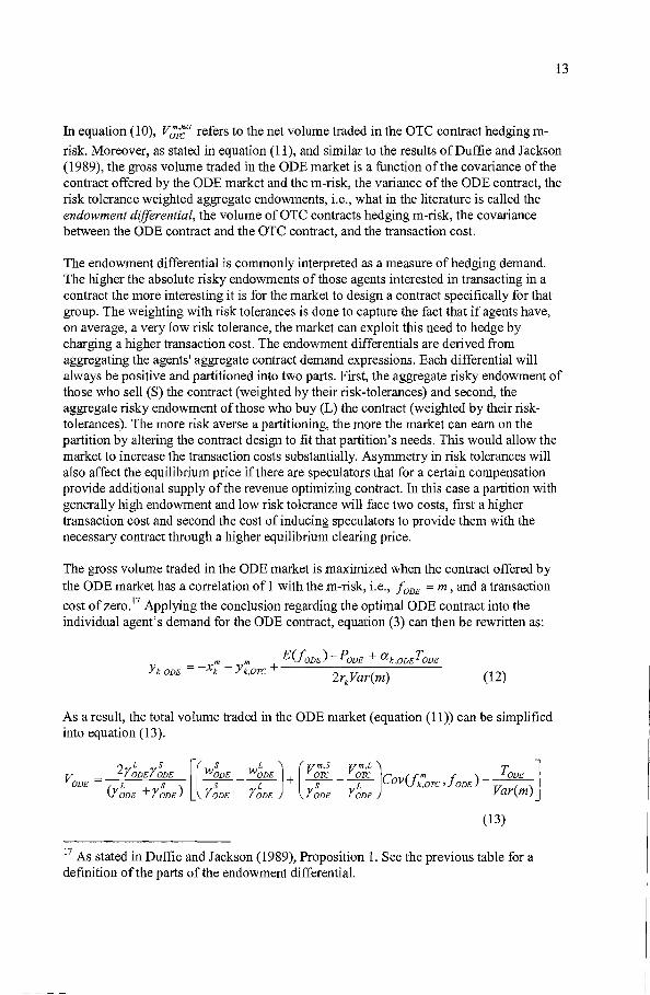
13

In equation (10), V;T~et refers to the net volume traded in the aTe contract hedging m­

risk. Moreover, as stated in equation (11), and similar to the results ofDuffie and Jackson(1989), the gross volume traded in the ODE market is a function of the covariance of thecontract offered by the ODE market and the nl-risk, the variance of the ODE contract, therisk tolerance weighted aggregate endowments, i.e., what in the literature is called theendowment differential, the volume ofaTe contracts hedging m-risk, the covariancebetween the ODE contract and the aTe contract, and the transaction cost.

The endowment differential is commonly interpreted as a measure ofhedging demand.The higher the absolute risky endowments of those agents interested in transacting in acontract the more interesting it is for the market to design a contract specifically for thatgroup. The weighting with risk tolerances is done to capture the fact that if agents have,on average, a very low risk tolerance, the market can exploit this need to hedge bycharging a higher transaction cost. The endowment differentials are derived fromaggregating the agents' aggregate contract demand expressions. Each differential willalways be positive and partitioned into two parts. First, the aggregate risky endowment ofthose who sell (S) the contract (weighted by their risk-tolerances) and second, theaggregate risky endowment of those who buy (L) the contract (weighted by their risk­tolerances). The more risk averse a partitioning, the more the market can earn on thepartition by altering the contract design to fit that partition's needs. This would allow themarket to increase the transaction costs substantially. Asymmetry in risk tolerances willalso affect the equilibrium price if there are speculators that for a certaIn compensationprovide additional supply of the revenue optimizing contract. hl this case a partition withgenerally high endowment and low risk tolerance will face two costs, first a highertransaction cost and second the cost of inducing speculators to provide them with thenecessary contract through a higher equilibrium clearing price.

The gross volume traded in the ODE market is maximized when the contract offered bythe ODE nlarket has a correlation of 1 with the m-risk, i.e., fODE = m , and a transaction

cost ofzero. 17 Applying the conclusion regarding the optimal ODE contract into theindividual agent's demand for the ODE contract, equation (3) can then be rewritten as:

E(!ODE)-PODE + a k oDEToDEm m + '

YIe,ODE =-Xk - Yk,OTC 2 T7" ( )rkrar m (12)

As a result, the total volume traded in the ODE market (equation (II)) can be simplifiedinto equation (13).

v - 2Y;DEr;DE [(W~DE _ W~DE J+ (Vo~~ _V;i~ JCOV{ I'm I' ) _ T ODE ]ODE - ( L s) S L S L J Ie ,OTC , J ODE ( )

rODE +rODE rODE rODE rODE rODE Var m

(13)

17 As stated in Duffie and Jackson (1989), Proposition 1. See the previous table for adefinition of the parts of the endowment differential.

14

The variable of choice for the ODE market is, therefore, only the transaction cost thatmaximizes the ODE market's revenue. Clearly, trading volume is maximized with atransaction cost of zero, the socially optimal solution if there would be only one market,since risk is shared to the largest extent possible across agents. In a single market setting,the ODE market would, of course not, choose such a transaction cost since its revenuewould also be zero. Hence, the ODE market faces the following maximization problem(by substituting equation (13) into equation (6)):

MAXTODE

T 2r~DEr~DE [(W~DE _ W~DE J+( VO~~ _ V;T~ Jcov( I'm I' ) _ TODE ]ODE ( L S) S L S L J k,OTC' J ODE T7 ( )

YODE + rODE rODE rODE rODE rODE y ar m

(14)

Maximizing equation (14) the ODE market faces a trade-off between the revenuesstemming from an increase in the transaction cost and the resulting decrease in tradingvolume. Moreover, the introduction of inter-market competition results in a particular andnew shape to how transaction costs affect a market's revenue. Solving the maximizationproblems in (14) for the optimal transaction cost yields equation (15).

T* = var(m)[(W~DE _ W~DEJ (V;T~ _ V;T~JC (I'm I' )]ODE 2 S L + S L OV J k,OTC , J ODErODE rODE rODE rODE

(15)

The optimal transaction costs for the ODE market is increased by a higher variance of theunderlying risk it hedges, i.e., given that agents are risk averse they are more willing topay a higher cost for their hedges. Similarly, the larger the absolute value of the riskweighted endowments of those that trade in the ODE market, the greater the potential forthe ODE market to charge a higher transaction cost. As expected, equation (15) alsoshows that competition with the OTe contract that hedges m-risk, limits the optimaltransaction cost charged by the ODE market (since the parenthesis with the volume ofaTe contracts traded sunlS to a negative number). Plugging, the optimal transaction costsinto equation (14) generates the following revenue function for the ODE market:

L S [( S L J (Vm,S Vm,L J ]R = T r ODEYODE WODE _ WODE + OTC _ OTC COV( I'm I' )ODE ODE ( L S) S L S L J k,OTC' J ODE

rODE + rODE rODE rODE rODE rODE

The OTC Market's Maximization Problem

(16)

The derivation of the ODE markets revenue function was relatively straightforward, sincethe ODE market only functions as an intermediary taking no positions of its own andcharges an up front transaction cost. However, as shown in equation (16) the ODEmarkets' revenue depends on the design of the aTe contract hedging m-risk and theamount that agents already hedge in the OTe market. A key addition of this chapter is theintroduction of a conlpeting market that has a different structure than the traditional ODEmarket. As noted earlier, the aTe nlarket will take positions of its own and therefore it isto a certain extent playing a role similar to the speculator in the ODE market case. The

15

aTe market's objective is to optimize risk-adjusted revenues rather than revenues per se,i.e., it is assumed that the aTe market maximizes a mean-variance type utility functionsimilar to that of the agents, but with risk aversion rOTC. afcourse, there is a limit to how

much market risk the aTe market can take on. This limit, which could be seen as themaximum value-at-risk an institution is prepared to take, or its net exposure in aggregateto market risk, puts a constraint on how much total risk the aTe market can hedge. Giventhis constraint the aTe market has an incentive to exploit those agents who have aparticular high risk aversion and/or a high level of idiosyncratic risk endowment that canonly be hedged through a customized contract. It is, therefore, assumed that the aTemarket maximizes the following mean-variance utility function:

UOTC (WOTC ) =E(wOTC ) - rOTCVar(wOTC)

s.t. WOTC ~ Q

(17)

In the above utility expression WOTC expresses the net revenue expected by the aTemarket from providing the various contracts to the interested agents. The total marketexposure the aTe market can take on is limited by some arbitrary amount Q. If n issufficiently low compared to hedging demand among the agents the market exposureconstraint will be binding. I8 Assuming, that the aTe market offers one contract to hedgeagents' m-risk, and up to K different customized contracts to hedge an agent's ek -risk,

WOTC would take the following form:

WOTC = LY~~OTC(Pk~OTC -E(f:'OTC))+ LY:,OTC(Pk~OTC -E(fk~OTC)) (18)keK keK

The aTe market's maximization problem could be expressed as in equation (19).

subject to:

LY~OTC (Pk~OTC - E(ft'~OTC))+ LY:,OTC (Pk~OTC - E(fk~OTC)) ~ QkeK keK

(19)

To solve equation (19), a lagrangian function is set up and the lagrange multiplier is used( ILk) for agent k, assuming that the budget constraint is binding for the aTe market when

supplying a contract to that particular agent. The variance part of equation (19) treats m-

18 An alternative budget constraint, which would be more closely related to a value-at-risktype set up, could be to put an upper linlit on the variance of the aTe market's totalmarket exposure. Such a limit would, however, unnecessarily complicate the subsequentderivation without much additional insight.

16

risk differently to e-risk. The formulation captures that the aTe market can net out m­risk by taking offsetting positions, but e-risk is individual to each agent and can thereforenot be netted similarly. Hence, regarding m-risk it is the net variance that matters for theOTe market. While equation (19) looks fairly complex it can be substantially simplifiedby carrying over the conclusions regarding the optimal contract design from the ODEmarket, i.e., the optimal contract is the contract that hedges the agents' risk the closest. 19

This implies that the optimal contracts for the aTe market are given and what remains todo is to solve for the optimal contract prices and the resulting OTe market risk-adjustedrevenue.

It is also assumed that while the idiosyncratic risks and their expected pay-offs would bedifferent across the agents, the variance of these pay-offs would be the same, i.e.:

As a result of these definitions, the demand functions for the aTe contracts, seeequations (4) and (5), can be rewritten as:

(4')

(5')

Substituting the revised demand expressions (including the expression for Yk,ODE , which

is also a function of P;'OTC) into (19), the optimal prices for the aTe market regarding the

contracts fo~c and f:OTC can be derived.

Pt:OTC :::: E(fo~c) + 2Var(m)(CkY~OTC + rOTC LY;OTC]l-Ak keK

=E(fo~)+2var(m{CkY;OTC+l~~k v;~et]

P,,~OTC =E(RoTC) + 2Var(e{rk +ck + 1~~k }:,OTC

(20)

(21)

19 This fairly straightforward result was shown in more detail and discussed in an earlierversion of this paper, but was left out in the current version for the sake ofbrevity. Thederivation is available from the author upon request.

17

As can be seen from equations (20) and (21), the price the aTe market chooses isbasically the expected value of the contract's pay-offplus a premium/discount, which isdirectly related to the variance of the underlying risk, the number of contracts bought bythe agent, and the agents' extra risk aversion for trading in an aTe contract. Contrary tothe aDE market, where there is one price at which everybody trades, the aTC market cancustomize its price for each individual agent. hl the case of the contract hedging m-risk,the price also reflects the aTC nlarket's net position. If the demand by agent k reducesthe aTe 11larket's net exposure to m-risk it will quote that agent a nlore favorable price(last term in equation (20)). Correspondingly, if agent k increases the net exposure of theaTe market, the premium charged to the agent will increase.

Due to the competition between the two markets there is an upper bound for the price theaTC market can charge for its fo~c contract, which is equal to the price in the aDE

market plus the transaction cost TODE ' To further exemplify how the aTC market sets the

price, consider the case where the aTC market wants to buy an m-risk contract fronl anagent, the market has to then compensate the agent for the counterparty risk, representedby c, which the agent is assuming by transacting with the aTC market. lfthe agentwould have sold the same amount of the aDE contract, the counterparty risk would notbe present given the clearing function the aDE market provides.

The prices of the contracts are also related to the lagrangian Ak when the constraint is

binding and reflects the choice of the aTe market of taking on m-risk through the sale orpurchase of a contract hedging m-risk or whether it makes more sense for the aTCmarket to use its finite capacity for market risk to sell or purchase the customized contracthedging the idiosyncratic risk. The relevant lagrangians for the aTe contract hedging m­risk and the one hedging e-risk can be derived by solving (20) and (21) with respect to Ak

and setting them equal to each other.2o The revised price for the aTe contract hedging n1­risk becomes:

While the price for the fk~OTC contract becomes:

Pk~OTC = E(fk~OTC) + 2Var(e)YZ,OTc(rk + ck + v:,net (Pt~J1'C - E(fo";.d - 2Var(m)ckY;oTJIOTe )

(23)

20 The derivation for the Ak s assumes that the aTC market ranks the agents and their

denland to transact by the profitability each transaction generates for the market. At somepoint, i.e., Q, there is a limit for the aTe market to take on extra risk. At that limit andfor that particular agent affected at that limit, Ak is different from zero and affects the

pricing decision for both the contract hedging m-risk and that hedging e-risk.

18

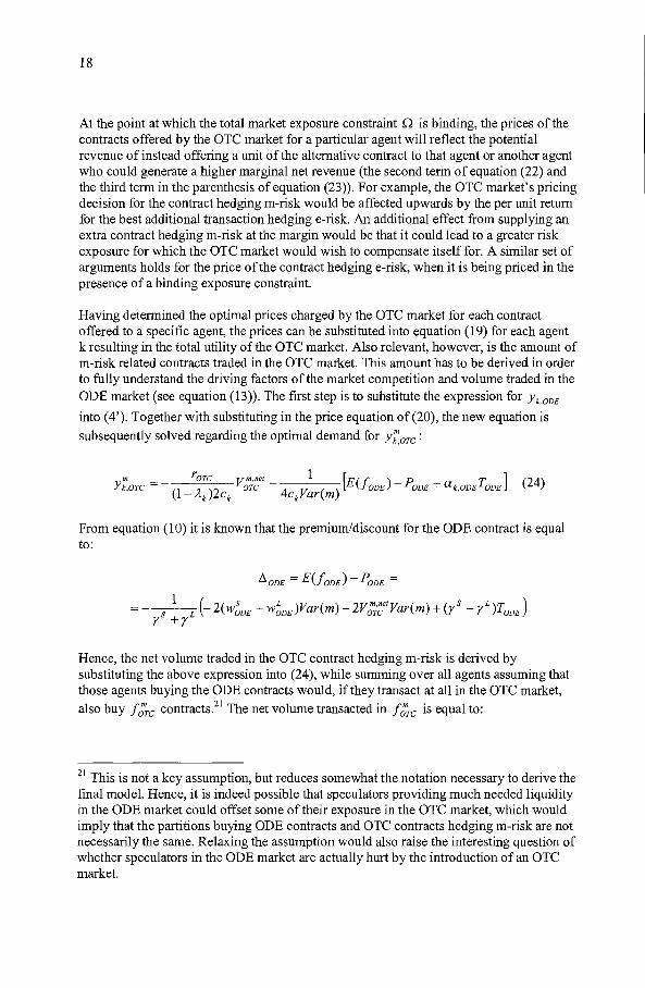
At the point at which the total nlarket exposure constraint n is binding, the prices of thecontracts offered by the OTC market for a particular agent will reflect the potentialrevenue of instead offering a unit of the alternative contract to that agent or another agentwho could generate a higher marginal net revenue (the second term of equation (22) andthe third term in the parenthesis of equation (23)). For example, the OTe market's pricingdecision for the contract hedging nl-risk would be affected upwards by the per unit returnfor the best additional transaction hedging e-risk. An additional effect from supplying anextra contract hedging m-risk at the margin would be that it could lead to a greater riskexposure for which the aTe market would wish to compensate itself for. A sinlilar set ofarguments holds for the price of the contract hedging e-risk, when it is being priced in thepresence of a binding exposure constraint.

Having determined the optinlal prices charged by the aTe market for each contractoffered to a specific agent, the prices can be substituted into equation (19) for each agentk resulting in the total utility of the aTe market. Also relevant, however, is the amount ofm-risk related contracts traded in the aTe market. This amount has to be derived in orderto fully understand the driving factors of the market competition and volume traded in theODE market (see equation (13)). The first step is to substitute the expression for Yk,ODE

into (4'). Together with substituting in the price equation of (20), the new equation is

subsequently solved regarding the optimal demand for Y;OTC:

m _ rOTC V m,net _ 1 [E( I' ) - P +aT] (24)YIe,OTC - (I-ILk )2c

kOTC 4c

leVar(m) J ODE ODE k,ODE ODE

From equation (10) it is known that the premium/discount for the ODE contract is equalto:

~ODE = E(!ODE) - PODE =

S 1 L(-2(W;DE +w~DE)Var(m)-2V;::etVar(m)+(rs -rL)ToDE )r +r

Hence, the net volume traded in the aTe contract hedging m-risk is derived bysubstituting the above expression into (24), while sun1ll1ing over all agents assuming thatthose agents buying the ODE contracts would, if they transact at all in the OTC market,

also buy !:;TC contracts?1 The net volume transacted in !:;TC is equal to:

21 This is not a key assumption, but reduces somewhat the notation necessary to derive thefinal nlodel. Hence, it is indeed possible that speculators providing much needed liquidityin the ODE market could offset sonle of their exposure in the aTe market, which wouldimply that the partitions buying ODE contracts and aTe contracts hedging m-risk are notnecessarily the same. Relaxing the assunlption would also raise the interesting question ofwhether speculators in the ODE market are actually hurt by the introduction of an aTemarket.

19

V m,net ~ m Vm,L + Vm,SOTC =: L...J Y k ,OTC =: OTC OTC

kEK

As shown above, the net volume traded is simply the volume of those agents buying the

f;TC contract and the others who are selling it.

V m,L ~ m rOTC (vm,L Vm,S) ~ 1 _ (Ll ODE - TODE ) ~OTC = L...JYk OTC = --- OTC + OTC L...J ( ) L...J

kELm.OTC ' 2 kELm.OTC I-Ak Ck 4Var(m) kELII/,OTC Ck

Vm,S = ~ym =_rOTC (Vm,L +Vm,S) ~ I _ (~ODE + TODE ) ~ ~OTC L...J k,OTC 2 OTC OTC L..J (1 A) 4V; () L....

kESm,OTC keSm,OTC - k Ck ar m keSm,OTC Ck

vm,net _ rOTC (r;T~ + r~;c) (vm,L + Vm,S) _ (r;TC +- r~TC )~ODE + (r;TC - r~TC )TODE

OTC - 2 OTC OTC 4Var(m) 4Var(m)

(25)

Solving equation (25) for the net volume traded in the aTe contract hedging m-risk,

while defining r OTCS as the sum of the different buy and sell partitions' tolerance to aTecredit risk, and whether or not the market exposure constraint is binding, the net volumeexpression can be expressed as in equation (26).22

V m,net _OTC -

(26)

Knowing the net volume traded in the aTe markets allows for the derivation of the grossvolume by noting that:

Similarly, the volunle of those buying and selling the aTe contract hedging m-risk has,as previously noted, an impact through the competition dimension on the amounttransacted in the aDE contract (see equation (13)). While, a later section will discuss inmore detail the key comparative statics of the model conclusions, equation (26)demonstrates that the higher the aTe market's or the agents' risk aversions are towards(i.e., the lower the aTe markets risk tolerance, rOTC' the smaller the r s, and the higher

22 Note that if there is no constraint on the aTe market's ability to take on risk, or ifit is

not binding, r~;c + rgT~ would be equal to r~TC + rgTC '

20

the agents credit risk aversion, Ck ) trading aTe contracts the less will be traded aTe and

demand is shifted to the ODE market. an the flip side, the higher the transaction cost inthe aDE nlarket, the more hedging demand will shift to the aTe market and trigger anincrease in trading volume in its m-risk contract. Interestingly, the higher the variance ofthe lmderlying risk the lower is the volume traded in the aTe contract hedging m-risk.This is so, since the agent's aversion towards trading the aTe contract is directly relatedto the underlying variance and therefore its credit risk. Hence, a nice result of the model isthat it shows that trading on a market where the contracts are cleared and where there isno counterparty risk is especially attractive for agents' with higher risk endowments.

The total volume traded of fk~OTC is much more straightforward to derive, since there is

no competition dimension. By substituting the optimal price of the aTe contract hedginge-risk (equation (21) into the agent's optimal demand expression (equation (5 ')) the

trading volume in f;OTC would be equal to:

yZ,OTC =

The total volume traded in the aTe contract hedging e-risk is derived by simplysumming the above expression across all agents23

, i.e.,

ve Ve,L Ve,s '"" e '" eOTC = aTC - aTC = LJYk,aTc - L...JYk,aTc =keLe,OTe keSe,OTe

Equation (27) shows the effect of summing individually customized contracts across allthe K agents. Given that volume traded by each agent is linked to each individual's riskand credit risk aversions and endowment of their own idiosyncratic asset, it is hard tosimplify (26) much further. There is a potential intra-aTe market competition dimension,which is related to the constraint on the aTe market's total market exposure discussedearlier (the link, for example, affects the price of the aTe contract, see equation (23)).Depending on whether or not the constraint is binding for the marginal aTe contracthedging m-risk or e-risk, a relaxation of the constraint could have an impact on thetransaction volume in the aDE market. This relationship is discussed in more detail in thenext section.

As noted earlier, contrary to the aDE market, the aTe market does not maximizerevenue, but risk adjusted utility. Hence, after the optimal prices for the two types ofcontracts the aTe market offers each agent have been determined, and the corresponding

23 The volume traded is a positive number since those agents' with a negative endowmenttend to buy the aTe derivative, i.e., V;T~ is positive.

21

transaction volumes derived, they can be plugged back into the original utility function ofthe aTe market (equation (19)). To reduce the notation below, the variance constraint isbriefly assumed to be not binding. This allows the following expression for the utilityfunction of the OTC market.

UaTC == U;;TC + U~TC =

var(m)(2LCk (Y;OTC)2 +raTC(VO~~etYJ+ (28)keK

+ var(e)(2LCk (yZ,OTC)2 + 2Lrk (yZ,OTC)2 + rOTC L (YZ,OTC )2JkeK keK keK

IV. COMPARATIVE STATICS AND MODEL RESULTS

An important driving factor in the model is that the OTC contract can also hedge risksthat the ODE contract can never address. This asymmetry provides interestingcompetition questions. For example, what is the volume traded in the ODE market inequilibrium, which market will have the lowest price/transaction cost, and how muchdoes competition increase/lower the socially optimum volume of trading? Since inoptimum both markets offer contracts that are perfectly correlated with the underlyingrisky endowments, the main channel of competition is the cost of completing eachtransaction more broadly. As a result, the optimal transaction cost expression for the ODEmarket has evolved in comparison to the previous literature, while the aTC marketcompetes by price and discrin1ination between agents.

A. Comparative Statics

Increased competition, through a higher trading volun1e in the OTC market's contracthedging m-risk, will decrease the level of the ODE market's optimal transaction cost.Hence, in a non-competitive setting, where there is only one monopolistic financialmarket providing only contracts hedging m-risk, the optimal ODE transaction cost wouldbe higher (see appendix for some numerical examples). For the OTe market, however,the choice is whether to use its scarce capacity to take on risky positions that are relatedto m-risk or whether it should only focus on providing a hedge against e-risk.

22

Table 3. Comparative Statics ofThe Model

rk Ck rOTC TODE Var(m) Var(e) vm,netOTe

Yk,ODE

Y~~OTe sign( v~~~et) ? -sign( V;T~et ) +

Y:,OTe + +

TODE +PODE +

Pk":oTe + ? + ? +

~'~OTe? + + +

vm,llet -sign( v~~~et) -sign( Vom,;~et) ? ?OTe

VODE ? + + +

vm,gross ? +OTe

RODE ? + + ?

UOTC + + + ?

Note: (..) implies that the comparative static is not relevant. (+) implies that an increase in a row headingcauses an increase in the column heading. (-) implies that an increase in a row heading causes a decrease inthe column heading. (?) implies that the sign is ambiguous and depends on the parameter values.

In the model developed in the earlier sections, the OTe market has an obvious advantagein that it can hedge an orthogonal risk that the ODE market can never capture with itscontract. Hence, in the absence of competition, the OTC market would provide theoptimal contracts for both types of risks. An implication of this competition is that theODE market's transaction costs, e.g., exchange and clearing fees, have to respond to thepresence of a competing market and be reduced. Hence, the ODE market competes, allelse being equal, through lower transaction costs. However, the relationship between thedifferent markets' transaction costs also depends on the structure of the endowments ofthe agents. Moreover, in a related decision, the aTe market has to decide to what anextent it wants to act as a "speculator" and take a net positive/negative position in m-risk

( Vo~~et). The fact that it is willing to provide "liquidity" by helping to address any

supply/demand imbalances in the endowment of the m-risk asset n1eans that the price atwhich agents transact in the ODE market actually declines. In the absence of this"speculator" function, the price at which the ODE market clears is higher (if it is assumedthat there is a net negative endowment ofm-risk) than if some of the excess demand forhedge is covered through the OTe market.

Turning to the comparative statics in more detail, as can be seen in the table above, thehigher the underlying variance ofm-risk the higher the optin1al transaction cost andtrading volun1e and hence revenue for the ODE market. Hence, standardized derivativeshedging endowments of a high variance are ofparticular attraction to the ODE marketfacing a competitive threat fron1 the OTe n1arket. For the aTe market the relationshipbetween the variance ofm-risk and trading volume is negative. This partly reflects, for aconstant ODE transaction cost, the credit risk aversion agents face when transacting in the

23

aTe market. Moreover, the OTe market's own risk aversion plays a role and affects theutility negatively ofproviding a contract hedging m-risk. An interesting result of themodel is that the bid/ask spread the aTe market charges for the contracts hedging m-riskis in the optimum the same as the transaction cost of the contract offered by the ODEmarket.24 lfthere was no competition from the aDE market, however, both the optimaldemand for the aTe contract hedging m-risk and the bid/ask spread would be different(see below, modifies equation (24)).

rY

m,nocomp _ _ xm kk,OTC - k 2

rk + ck

If it is assumed that the risk and credit aversions of the agent going long the aTe contracthedging m-risk are the sanle as those of the agent going short the contract the bid/askspread in a non-competitive setting is equal to:

Pm pm 2Var(m)c( m m) h (m m) 0L OTC - S aTC = X S - XL were X s - XL>, , r+2c

This bid/ask spread, depending on the gross endowments of the two agents going longversus short can be bigger or smaller than the aDE market optimal transaction cost in acompetitive setting.

Tunling to the variance of e-risk, the effect of a higher variance is the reverse ofwhat it isfor the aTe market in terms of m-risk. The intuitive reason for this result is that the aTenlarket is exploiting its monopoly power as much as possible in the e-risk market. Since itis the sole provider of an instrument to hedge the idiosyncratic risk, it can ask a high pricefor that service. Of course, a side effect of entering into a lot of fairly rewarding contractshedging agents' individual e-risk is that the variance of those positions quickly add upand do not net out in the same sense as the positions the aTe market enters intoregarding m-risk (where it is the net position that matters for the aTe market's own riskaversion). lfthe aTe nlarket has a high level of risk aversion it would shift more of itsexposure and transaction volume to the contract hedging m-risk than to the contracthedging e-risk. For example, if the aTe market's risk aversion is very high it can stilltransact in the m-risk market, while setting its net exposure to zero. af course, the sideeffect in this case would be that the equilibrium price charged by the ODE market

24 Assume two agents, one that wants to buy the aTe contract hedging m-risk and onethat wants to sell the contract. The bid/ask spread is derived by subtracting the pricecharged by the aTe market to the seller from that charged to the buyer. By substituting inthe agents optimal demand/supply it turns out that the optimal bid/ask spread that theaTe market charges is the transaction cost charged by the aDE market. Hence, as thetransaction cost in the ODE market is increased it is optimal for the aTe market to followsuit, i.e., it chooses to not compete on price. This argument assumes that the endowmentof the agent trying to sell m-risk and that of the agent buying m-risk is the same with thesigns reversed. Also they must have the same risk aversions and the exposure constrainthas to be non-binding.

24

increases since the aTe market would not play any market maker function by assumingnet risk. In such a setting, the aTe market nlay therefore be unwilling to transact in anyaTC contract hedging e-risk or only at such a high cost that agents do not want to hedgethese risks (see the appendix for a quantification of this example). Such an outcome,driven by high aTC nlarket risk aversion, would have fairly large negative welfareeffects.

B. Additional Model Results

So far the downside of customization has not been discussed in detail. Customizationleads to an accumulation ofcredit risk, because neither the agents nor the OTC marketcan normally hedge their credit (or counter party) risk. Accumulating credit risk is clearlycostly to the agent and the issuing aTe market. In the case of the ODE market, however,credit risk is managed with through the clearing system. Agents transacting in the OTCmarkets do not generally have access to such clearing facilities. Therefore, it is reasonableto assume that in the case of the OTC markets, the more customized a contract is, and thehigher its market value, the larger the subsequent credit risk exposure faced by the agentand the issuer. Customization also limits the possibility of a resale if the counterpartydefaults. However, in the global OTC interest rate and foreign exchange swap markets,recently evolving bilateral and multilateral netting arrangements are potentially anefficient way to decrease the credit risk faced by a single participant.

Regardless of the ways in which the agents transacting in the OTe market try to mitigatetheir credit risk exposure, the maximum possible unhedgeable loss to the agent, i.e., thenumber of contracts multiplied by the contract's payoff, will be a key variable in theagents' utility functions. In general, agents (as well as the aTe market) have to set asidecapital against their net OTC counterparty exposure; in the case of international banks itwould depend on the nlaximum loss according to the traditional BIS rules. Setting asidecapital is costly, since it is not generating as much return as it could. Therefore, creditexposure incurs a cost for the issuing bank or organization. Several ODE markets arestarting to offer successful ways for reducing the credit risk costs faced by the aTemarkets by offering them tailor made clearing services.25 This fairly recent strategyexploits the ODE markets' long experience with clearing. According to a recent BIS(1998) publication, several additional derivatives exchanges have recently announced theset up of clearing facilities for less exotic aTe contracts.

hl the model developed in this chapter, some of the costs of customization are modeled byincluding the aTe market's general risk aversion ( raTe) and the agents' specific

individual credit risk aversion, ck • Increased levels of credit risk aversion among agents

have a direct negative effect on their demand for OTC contracts. O-iven the presence ofcompetition in the case of the OTe contract hedging m-risk, a change in the credit risk

25 Several clearing houses have been set up recently to clear fairly standardized OTetransactions, e.g., Brazil BM&F, Sweden's OM's Tailor Made Clearing, and the LondonClearing House's Swapclear. For more information see BIS (1998) and the President'sWorking Group on Financial Markets (1999).

25

aversion parameter does not change the OTe market's optimal bid/ask spread, which isstill equal to the ODE market's transaction cost, but rather affects transaction volume.Similarly, the price spread for agents' hedging their e-risks, while having similarendowments and risk aversions, is also unchanged. Hence, the transaction demand forOTe contracts is rapidly affected negatively and the effect is especially pronounced forthe aTe contracts hedging e-risk, given the higher marginal utility which the OTemarket derives from this market due to its monopolistic position. The ODE market,however, clearly stands to gain from the loss in competitive pressure from the aTemarket and both ODE market revenue and volume would respond positively. The overallutility of the agents trying to hedge their risks suffers, however, since the positive effectofmarket competition on prices and transactions costs is eroded.

One remaining and related variable requiring analysis is the importance played by themarket risk exposure restriction Q and its interplay with the other key variables, such asoverall risk and credit risk aversions. Equation (19) illustrates how the OTe market'sability to accumulate market risk is limited. Depending on the size of the limit, thisrestriction will force the aTe market to make a decision between providing aTecontracts hedging m-risk or e-risk. In essence, this constraint implies that the aTe markethas to rank each potential transaction by the utility it creates and then select the contractsthat provide the highest utility, whether they are hedging m or e-risk. If Q is set highenough, i.e., the constraint is largely non-binding, then Ak = O'v'k and the aTe market

can maximize freely (as is assumed in the numerical examples in the appendix). The moreinteresting case is when the constraint is sufficiently binding and the aTe market's riskaversion is high. In such a scenario, the market is now maximizing within the constraintand will provide mostly contracts hedging m-risk. If, however, the constraint was bindingin the context of low aTe market risk aversion, the aTe market would largely only haveprovided contracts hedging e-risk. These results are, however, largely driven by theassumptions made with respect to the associated parameter values for the constraint andthe risk aversions. All the same, they demonstrate that when assuming an economicallybinding constraint, the lower the aTe market's risk aversion, the more it will providehedge for those agents with e-risk. This also means that in the case of the aDE market,and as noted in equation (14) and (16) and Table 3, its trading volume and revenue willincrease when the risk aversion for the aTe market declines.26 If, however, the riskaversion of the aTe market is very high while the budget constraint is non-binding it ispossible that small changes in the risk aversion will have no significant impact on thedegree ofcompetition with the aDE market. This is the case, when as above, the aTemarket decides to take a near net zero position in contracts hedging m-risk.

26 This can be easily seen from a comparative static sense by setting the r s equal to each

other. In that case, the gross volume traded in the aTe contract hedging m-risk directlydecreases overall ODE trading volume, optimal transaction cost, and, as a result, aDErevenue.

26

v. ANALYSIS AND POLICY IMPLICATIONS

The first implication of the model is that introducing an interrelationship between twodifferent derivatives markets, fundamentally changes the behavior ofboth the aDEmarket and the aTe market. The new contracts launched by each market, and theirtransaction costs, now have to take into account the competitor's response. For the ODEnlarket, the optimal contract is still of the classic Duffie and Jackson (1989) type, i.e.,strictly geared towards hedging systematic risk. However, the aDE market's optimaltransaction cost now reflects a conlpetition dimension. A second implication is that theoptimal transaction costs and prices for both markets are critically dependent on theagents' initial endowment structure. Moreover, an ODE market competes preferably withtransaction costs, while the aTC market selects to launch an aTe contract hedging m­risk at a price that in the optimum situation does not outconlpete the ODE market. Hence,in equilibrium, both contracts will face some demand and both playa useful role innlaximizing the transaction volume, lowering monopoly rents, and increase the degree ofsocially optimal hedging.

The model also recognized the counterparty credit risk, stemming from the costs ofcustomization, leading to some interesting implications. Increased credit risk aversionamong agents decreases the demand for customized OTe contracts and reduces thebeneficial impact on the agents of introducing competition between markets. Moreover,the interrelationship between the aTC market's risk aversion and its market exposureconstraint is such that a reduction in risk aversion may allow the aTe market to focusmore on providing agents with a hedge for their e-risk rather than hedging their m-risk.This leads to an important insight, i.e. an ODE market has at least three options forresponding to the competitive threat posed by the aTe markets. Firstly, it can decrease itstransactions costs. Secondly, it could target only endowments with a very high variance.Thirdly, it could reduce the cost to the OTe market of customizing aTe instruments byproviding efficient clearing services thereby reducing the aTe markets overall riskexposure. The third option is in line with recent initiatives by several ODE markets ofintroducing tailor made clearing services for sonle aTe contracts. This means that therapid growth of aTe markets does not need to necessarily be a threat to those ODEmarkets that are quick to adapt by providing clearing services thereby growing with theOTC markets. However, there are other altenlatives for the aTC market. Kroszner (1999)discusses an alternative mechanism, the so called derivative product company (DPC),through which participants in the aTC markets can limit counterparty risk. DPCs aregenerally separately capitalized special purpose vehicles with a high credit rating and areset up by one of the international banks. A significant share of the international banks'aTC transactions are already chamleled through DPCs, (see Kroszner (1999) for a moredetailed discussion), ensuring that any counterparty risk for the bank is with the DPe andthat of the end-user is with the DPC as well. While the DPe approach mimics to a certainextent a clearing structure, it does not net credit risk exposure for the banle Its main usehas rather been to ensure that international banks with a relatively low rating can still takepart in the aTe market through these special purpose vehicles. As a result, the use ofDPCs has dinlinished over the last few years as banks have attained a higher credit rating.

Perhaps any corporate entity could potentially provide clearing services without being inan aDE market itself. Perhaps this is true, but existing ODE nlarkets are likely to bothbenefit from significant first mover advantages and the fact that clearing is a business

27

with large economies of scale. Hence, there seems to be significant, if increasinglytapped, potential for ODE markets to evolve into clearing specialists, off loading andeffectively managing the risks taken by aTe markets. From a supervisory perspectivesuch a development should be rather welcome, since the authorities' main concern hasbeen the systemic stability of the aTe market as a whole (see Schinasi and others, 2000).In the U.S. (see appendix II) voices have recently been raised for the regulation of theaTe markets and the deregulation of the ODE markets. This chapter suggests that inaddition to trying to deregulate themselves faster, ODE markets have other avenues toevolve their businesses, and supervisors could support the expansion, and spinning off, oftheir clearing businesses (perhaps) through regulatory incentives.

VI. CONCLUSIONS

The model presented in this chapter addresses the issue of the interrelationship betweentwo different markets, the ODE market and the aTe market. During the last few years,competition between these markets has grown more intense and ODE nlarkets areactively seeking alternative strategies to come to grips with the aTe markets. Theseinclude increased innovation, lower transaction costs, lobbying for the leveling of theregulatory and supervisory playing field, and launching clearing facilities for certain typesof aTe contracts.

This chapter models the main differences between these two markets as being differencesin the type of risk against which they can provide a hedge, their different risk aversions,and their ability for handling the agents' credit risk. The contracts considered aregenerally of a forward type that can either hedge systematic risk (m-risk) or an agent'sidiosyncratic risk (e-risk). The modeling framework introduced is an extension of theincomplete markets financial contract model originally developed by Duffie and Jackson(1989).

It is argued in the chapter that aTe and ODE derivatives markets can both complementand compete with each other. For example, the large broker/dealers of aTe derivativesfrequently rely on a liquid ODE market to dynamically hedge their market risk.Conversely, organized futures and derivatives markets in the U.S. face competitivepressure from OTe markets, which are offering fairly similar contracts but are largelyunburdened by regulatory and supervisory oversight. To a certain extent, competitionbetween aTe derivatives and ODE derivatives is detemlined by the structure of thecontracts and the type of risk end users want to hedge. Hence, it may be useful to analyzehow ODE markets can increase their comparative advantage in highly standardized, highvariance, and liquid derivatives while also providing clearing services for aTederivatives. In attempting to analyze how ODE markets can respond to the threat posedby aTe derivatives more research is, of course, needed to model the interrelationshipsbetween these markets. Although potentially a relevant area for future regulationinitiatives, very little research has yet been done on this topic. Rather, the main focus ofthe security design literature has been on competition between different stock exchangesor ODE markets.

This chapter takes a first step in analyzing inter-derivative market competition in amultiple contract setting. The nlain findings of this chapter are that the two derivativesmarkets can co-exist in equilibrium while exploiting their comparative advantages.

28

Competition is also clearly welfare enhancing and offers a better outcome for the agentstrying to hedge their m-risk or e-risk than in any single market setting. This result isshown to hold true even in a setting where the aTC market can issue multiple contracts,while the ODE market is limited to only one. Interestingly, to decrease competitivepressures, it is SOllletimes in the interest of the ODE markets to help reduce the aTemarkets' risk aversions. For example, in a U.S. setting (discussed in Appendix II) theODE markets could refrain from lending their support to an increase in regulatorypressure on aTe markets, potentially increasing the cost to the aTe market of offeringcustomized contracts. Instead, the most useful approach for ODE markets could be to dealwith the conlpetitive threat posed by aTe markets by lowering their transaction costs,targeting high variance assets, and introducing mechanisms that could help reduce thecounterparty credit risk which the aTC market takes on when transacting withcounterparties. The latter could be achieved, for example, by providing customizedclearing services, which would allow the aTe nlarket to better target those investors withparticular types of idiosyncratic risks.

For further research purposes, an empilical paper quantifying some of the assumptionsn1ade in this chapter would be very beneficial. While it is clear that competition betweenthe two market types is intense both in the United States and globally, from the aDEmarkets' perspective, there are no studies comparing the transaction costs of similar aTeand aDE derivatives. The lack of research in this area can probably be attributed to thedifficulty of collecting transaction data for the aTe markets that tends to be of aproprietary nature.

In summary, this chapter could serve as useful background material for understanding thecompetitive market microstructure between the two different market types. Consequently,it can serve as a first attenlpt to improve our understanding of the relationship betweentwo very important derivatives markets. Therefore, it is hoped that this chapter will helpinform policy discussions concerning the refonn and regulation of ODE and aTCmarkets, especially in the United States, and elsewhere.

29

APPENDIX 1. NUMERICAL EXAMPLES

This section presents a simple example of an economy consisting of 14 agents, derivingthe optimal transactions costs and the optimal aTe market behavior. The example willshow how the markets' revenues are affected by changes in transaction costs, riskaversions, and agents' endowments. The numbers and agent types are adapted fromTashjian and Weissman (1995).

Setup

The setup is the following, all the agents have the same risk aversion,

rk = 0.1,k = 1, ...,14

and the same aversion to credit risk (this will be changed in some examples), i.e.,

Ck = O.I,k = 1, ... ,14

Each agent is either endowed with either m or ek , or a combination ofboth. The two

endowment types are uncorrelated, andVar(m) 1

Var(ek ) 2

The variances are chosen in such a way that the idiosyncratic risk has a higher variance.

Table A.l. Initial Endowments for Each Agent of the Systematic Assetand the Idiosyncratic Uncorrelated Asset

Agent

1234567891011121314

Endowment ofm

50-100o

-3030-3030-3030-3030-3030-30

Endownlent of ek

oo

50-10030-3030-3030-3030-3030-30

The presented endowments do not net to zero when summed. This guarantees that, whilethe net supply of any ODE contract has to be zero, the aTe market plays a useful role inacting almost as a speculator by providing some of the supply to close the overall

30

demand/supply imbalance in contracts hedging m-risk. However, taking a net position isrisky for the aTe market and it is assumed that it is risk averse with rOTC = 0.05. To

avoid discontinuities in the figures it is also assumed that agents are sufficiently riskaverse not to play the role of a speculator and take positions that are of the same sign astheir initial endowments. Hence, all agents, with the exception of the aTe market, aretrading to hedge themselves.

Optimal ODE Market Transaction Cost

Figure A.I. shows the relationship between ODE market's revenue and volume versus itschoice of transaction cost. Initially a higher transaction cost more than offsets the declinein trading volume by generating higher per contract revenues. This works up to a certainpoint, as more and more agents choose to instead transact in the aTe market (the increasein trading volume of the aTe contract hedging m-risk) or reduce their overall hedgingdemand (total volume traded in m-risk declines throughout).

Figure A.I. Optimal ODE Market Transaction eost

700

800

900 ..,.------------------r--------.- 900- - - - OTe Market Utility ofm-risk contract_. - - - OTe Volmne Traded in m-risk contract--ODE Volume Traded--ODE Market Revenue- - Total Volume Traded in m-risk

700

800

600 +--------------_-~----' _ 600

500

400

300

200

500

400

300

200

2.92.52.11.71.20.80.4

" .- .- ~.: - - . - - - 1001" -.'''' .. _- .. ......,... -- J-!!!.. .-- - - --

o -+---'==--,---~-___r__-__r_--__r__-__,_--_r__-....J- 0

0.0

100

Transaction Cost in ODE Market

A higher transaction cost in the ODE n1arket also allows the aTe market to increase thespread it charges agents to take the offsetting long/short positions. As noted in thecomparative static section, the spread the OTe market charges is in optimum equal to thetransaction costs charged by the ODE market. Hence, gradually both volume and revenueincreases for the aTe market (volume increases linearly while utility rises more quickly).In this example the ODE n1arket would choose a transaction cost of slightly below 2.5 tomaximize revenues. The choice would mean that some transactions hedging m-risk arecompleted in the OTe market, since prices can be customized in that market as well.Hence, rather than to set a transaction cost low enough such that there are no transactionsin the aTe contract hedging m-risk the ODE market has some room to maneuver thanksto that trades in that market does not suffer from credit risk and that the market is riskneutral.

31

In the absence of an aTe market, Figure A.2 shows that the optimal transaction costwould be substantially higher at around 3.5. Since, the speculative position taken by theaTC market is no longer available, the price to clear the ODE market is also higher thanin the case of competition.

Figure A.2. Optimal ODE Market Transaction Cost IfNo Competition

900 .,.---------------------r 2.5

800 -... _ -.. __

-.. -700 - --... --....---. 2

600

5001.5

0.5

4.74.13.42.72.01.4

--ODE Vohnne Traded--ODE Market Revenue- - Pode (right scale)

0.7

-/'-----,---_r----.------r----r------,---.,----+O

400

300

100

200

Transaction Cost in ODE Market

As a result, the total volume traded is therefore higher in a scenario in which there iscompetition between the two markets, since the ODE market has to lower its transactioncost to compete more effectively.

Implications of Changing the Variance of m-risk

It was argued in the comparative statics section that the higher the variance ofm-risk theless beneficial it is for the risk averse GTe market to compete for transactions. To acertain extent this finding, while generally true, is subj ect to the assumption that there areno speculators with the exception of the aTe market itself.

Figure A.3. shows that the trading volume in the aTe contract hedging m-risk is strictlydecreasing as the variance ofm-risk increases. Meanwhile, for the ODE market thereverse is true and both revenue and the agents' hedging demand in the form of theirtrading volume is strictly increasing with the variance ofm-risk. While it is true that if thevariance ofm-risk is zero there is no transaction demand whatsoever for either contract,in this example since there is a fixed ODE transaction cost set at 0.25, the variancetherefore has to be above some minimum positive level to generate any demand for theODE contract. In the case of the aTe market, since it doesn't charge a transaction costper se but rather a bid/ask spread, it can still provide some hedge even if the variance ofm-risk is very low. For figure A.3. the ODE market transaction cost is held constant, butaccording to the modeling framework the ODE market would, of course, respond tolower nl-risk variance by lowering its own transaction cost and still generate somerevenue.

32

Figure A.3. Effect of Changing the Variance ofm-risk

600

700

600

700

800 .,....,--------------------,---------,- 800...... - OTC Market Utility ofm-risk contract

- - OT C Volume Traded in m-risk contract

---ODE Volume Traded

---ODE Market Revenue

500 500

100

200

400

300

100

200

-..... __ .....~..--:-:.~.-:-:-..-:-:_:-:-:.~._~.~._--.-o 00.15 0.30 0.45 0.60 0.75 0.90 1.05 1.20

400

300

Variance of rn-risk

By adapting to the lower variance ofm-risk, the ODE market can ensure that there is stillsome trading in the ODE contract (Figure A.4.). Only gradually will the ODE marketraise its transaction costs, while still ensuring the same level of trading volume. Since theOTC n1arkets optimal response is to set its bid/ask spread to the ODE n1arket'stransaction costs, its trading volume is also constant. Interestingly, and different to figureA.3. and the comparative static section, the OTC market's utility from offering a OTCcontract m-risk now increases with the variance ofm-risk (since higher variance increasesthe ODE market's optimal transactions costs, which allows the aTC market to widen itsbid!ask spread.

Figure A.4. Effect of Changing the Variance ofm-riskwhile allowing TODE to Change

800 .---------.--------~2.5

700

600

500

... - ... OTC Market Utility of rn-risk contract- - OTC Volume Traded in rn-risk contract---ODE Volume Traded---ODE Market Revenue- - - - Transaction Cost ODE Market (right scale)

1.5

400

300

200

100--------­.. -".---."., ... -

0.5

1.20

O+------r----,------,.----r-------,r------r---.,....--~O

0.15 0.30 0.45 0.60 0.75 0.90 1.05

Variance of rn-risk

33

Implications of the Credit Risk Aversion Dimension

The implications of including a credit risk dimension can be exemplified in the context ofredoing the earlier numerical examples. Fronl the analysis in the modeling section itwould be expected that the higher the agents' credit risk aversion the less they would liketo trade in aTe contracts hedging m- or e-risk.

The reasoning above, with respect to agents' credit risk aversion is shown in figure A.5.The trading volume in the aTe contract hedging m-risk declines rapidly as agents reactto the higher implicit cost due to their increasingly costly credit risk exposure.Simultaneously, the revenue and trading volume generated in the ODE market increaseswith a higher level of agent credit risk aversion, due to that market's ability to net outcredit risk through its clearing system. In light of the earlier discussion of transactioncosts, a side effect of higher credit risk aversion, is that the OTe market is less effectiveas a competitor. Hence, the ODE market's optimal transaction cost increases and the totalendowment ofm-risk that is hedged declines. This implies that the higher credit riskaversion has welfare implications from a pareto perspective, since it decreases theaggregate trading volume and thereby reduces the total utility for the agents. Anothersimilar effect, is that the higher credit risk aversion also reduces the OTe market'swillingness to act as a speculator by taking on net exposure. As shown in the figure thenet supply of contracts hedging m-risk declines rapidly.

Figure A.S. Effect of Changing Credit Risk Aversion

--- ..".,. -~.o:.~ .-..-:-:'.:".~ _~ .~.._. .""'I:"'!'.:'. ~.~."!:"O-t------,----r------r--_r------r----..,.----r-----L.O0.020 0.095 0.170 0.245 0.320 0.395 0.470 0.545

10

9

6

2--- ...... -.. .........

..... ---. ...........

....................

- - - OTe Market Utility ofm-risk contract....... OTe Volume Traded in m-risk contract--ODE Volume Traded--ODE Market Revenue- - - - OTe Net m exposure (right scale)

_--:~--------------1-4

800

700\\

600 \\

500

400

300

200

100 ."' ..'

Added OlC Market Credit Risk Aversion

Implications of Changing the Variance of e-risk and the OTC Markets RiskAversion

The previous examples have focused on the interactions between the OTC market and theODE market, but have left the trading volume of custonlized contracts hedging eachindividual's unique e-risk unaddressed (Figure A.6.). Taking into account the endowment

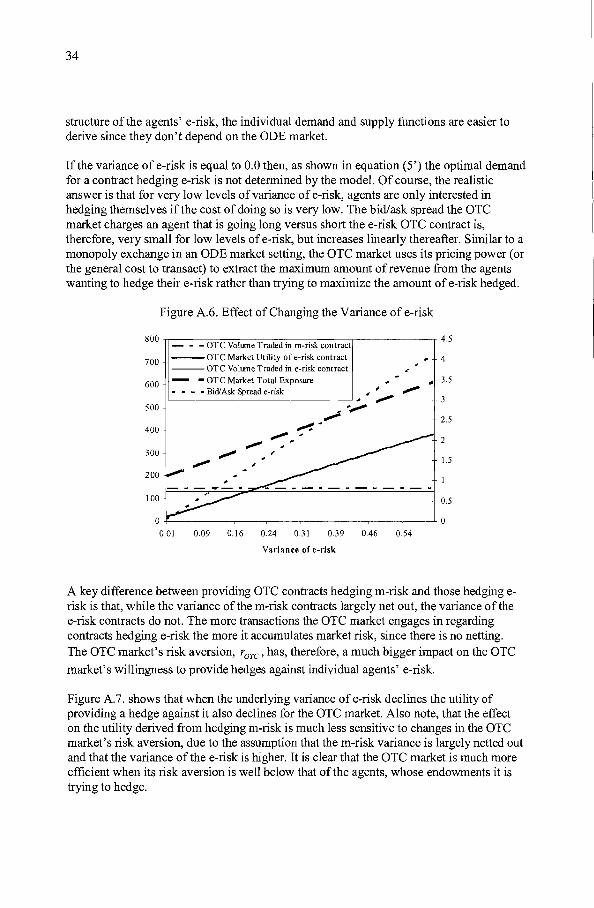
34

structure of the agents' e-risk, the individual demand and supply functions are easier toderive since they don't depend on the aDE n1arket.

If the variance of e-risk is equal to 0.0 then, as shown in equation (5') the optimal demandfor a contract hedging e-risk is not determined by the model. af course, the realisticanswer is that for very low levels ofvariance of e-risk, agents are only interested inhedging themselves if the cost of doing so is very low. The bid/ask spread the aTemarket charges an agent that is going long versus short the e-risk aTe contract is,therefore, very small for low levels of e-risk, but increases linearly thereafter. Similar to amonopoly exchange in an aDE market setting, the aTe nlarket uses its pricing power (orthe general cost to transact) to extract the maximum amount of revenue from the agentswanting to hedge their e-risk rather than trying to nlaxinlize the amount of e-risk hedged.

Figure A.6. Effect of Changing the Variance of e-risk

1.5

4.5

0.5

2.5

.. 3.5

~ 4

100

200

400

300

800 ------ - - OTC Volume Traded in m-risk contract

--OTCMarket Utility ofe-risk contract--OTC Volume Traded in e-risk contract

- - OT C Market Total Exposure

IL-_-_-_-_Bi_d/_A_sk_S_pr_ea_d_e-_ri_sk ; ., ~ ",

500 ~""~

~ ...

""*' '~ ;

700

600

O+-----,---.,..-----,...------,,-------.------,----,------L-

0.01 0.09 0.16 0.24 0.31 0.39 0.46 0.54

Variance of e-risk

A key difference between providing aTe contracts hedging m-risk and those hedging e­risk is that, while the variance of the m-risk contracts largely net out, the variance of thee-risk contracts do not. The more transactions the aTe market engages in regardingcontracts hedging e-risk the more it accumulates market risk, since there is no netting.The aTe market's risk aversion, rOTC' has, therefore, a much bigger impact on the aTe

market's willingness to provide hedges against individual agents' e-risk.

Figure A.7. shows that when the underlying variance of e-risk declines the utility ofproviding a hedge against it also declines for the aTe market. Also note, that the effecton the utility derived from hedging m-risk is much less sensitive to changes in the aTemarket's risk aversion, due to the assumption that the m-risk variance is largely netted outand that the variance of the e-risk is higher. It is clear that the aTe market is much nloreefficient when its risk aversion is well below that of the agents, whose endowments it istrying to hedge.

35

Figure A.7. Effect of Changing the aTe Market's Risk Aversion

600

800

- - - aTC Market Utility ofm-risk contract 1400- - ..... OTe Volume Traded in m-risk contract--OT C Market Utility of e-risk contract--OTe Volume Traded in e-risk contract 1200L--__-_O_T_C_M_a_rk_e_tT_o_ta_I_E_xp_o_sur_e__---+ 1000

600

800

1200

1400

400 400

200 :-:-:.~ .":":"'..-..~.~.:-:-:.": .":"":""..-..~.:'.:-:-:.":.77'..-..-:"":.:' ... _ 200

o a0.00 0.08 0.15 0.23 0.30 0.38 0.45 0.53

OTC Market Risk Aversion

Exposure Limits, Credit Risk Aversion and the Demand for e-risk hedge

As noted in the aTe market's utility expression there is a limit to the nlaximum marketrisk exposure (Q in equation (19)) the aTe market can take on. This assumption, asnoted earlier, intends to capture that there is some credit risk for the aTe market as wellwhen it assumes a lot ofmarket risk based on the bid/ask spread it charges agents timesthe volume it transacts with these agents. Figures A.6. to A.S. all show the total exposuregenerated by the aTe market selling/buying contracts in an unconstrained fashion(Ak = 0). Of course, if an overall constraint is introduced and the market exposure of the

aTe market exceeds this limit, the aTe market would have to discriminate betweenagents and only provide hedges to those agents adding the highest marginal utility.Depending on the variance of e-risk and m-risk and the agents' and the aTe market'srisk aversions, this may result in that either an aTe contract hedging m-risk or onehedging e-risk ends up being constrained and therefore not offered. The effect on theODE market depends on what contract is constrained at the margin. Ifits is a contracthedging m-risk then there would be an impact.

Moreover, the demand for e-risk hedged by agents is also affected by their credit riskaversion. Similar to the aTe contract hedging m-risk, increased credit risk aversionsamong agents have a large impact on the utility the aTe contracts generated by providinghedges. The volume ofaTe contracts traded that hedge e-risk is not affected as much,since rather than reducing the transaction volume the aTe market first reduces thebid/ask spread at which the agent can transact.

36

Figure A.8. Another look at the effect of Changing Credit Risk Aversion

1000

900

800

700

600

500

- - - OTe Market Utility ofm-risk contract. -. - .. - OTe Vohnne Traded in m-risk contract---OTe Market Utility of e-risk contract---OTe Volume Traded in e-risk contract- - OT C Market Total Exposure

0.17 0.25 0.32 0.40 0.47 0.55

400

300

200

100............

+---.------..----.---.-.,......-..-.-.-. .,....-.---.-."-.,......-.------r.---_-_.--L- 0

1000

900

800

700

600

500

400

300

200

"-100

0

0.02 0.10

Added OTC Market Credit Risk Aversion

37

ApPENDIX 2. REGULATORY AND SUPERVISORY TREATMENT OF OTe VERSUS

ODE DERIVATIVES IN THE UNITED STATES

The United States has some of the largest and most innovative OTC issuers, while alsobeing home to some of the world's largest ODE markets. Regulatory agencies, such as theCommodity Futures Trading Commission (CFTC), have generally been cognizant of thepotential competitive and systemic challenges posed by the aTC markets. However,rather than deregulate the ODE markets, much initial discussion dealt with tighterregulation and oversight of aTC markets.

The state of regulation globally with respect to aTe swaps and derivatives has beenuncertain ever since the birth of the OTC market.27 In the U.S., laws governing futurestransactions were last substantially revised in 1974, establishing the CommodityExchange Act (CEA) and the CFTC (8ee ISDA, 1999, and President's Working Group,1999). These laws were never sufficiently revised to provide the aTC market withregulatory certainty, and the specter of CFTC regulatory oversight remained, threateningthe legality of existing swap agreements and aTC derivatives. The illegal aspectoriginated when the CEA explicitly banned off-exchange "futures" contracts withoutdefining clearly what a "futures" contract was. Therefore, the lack of clarity of the CEAwas used by disgruntled investors, after losing substantial amounts ofmoney due to anOTC transaction, to claim that the transaction was illegal to begin with, therebypotentially nullifying the transaction and recovering their losses. A further result of thelegislation was that when the American organized derivatives exchange markets, such asthe CBOT and the CME, started to seriously feel the competitive pressure fronl the OTCmarket, they lobbied the CFTC to take action on OTC derivatives based on the CEA (seeSchinasi and others, 2000).

aTC market participants' sensitivities were further heightened when the CFTC in 1987started investigating commodity swaps originated by Chase Manhattan. No enforcenlentwas done but this move and some follow-up efforts forced much of the U.S. OTC marketoff-shore in response, stifling innovation and increasing costs. Pressure was subsequentlybrought to bear on the CFTC by the U.S. Treasury, the Federal Reserve and industrygroups, such as ISDA, to exempt some Swaps from the CEA and CFTC oversight, subjectto certain eligibility criteria. The.resulting "Swaps Policy Statement" stated that "at thistinle most swap transactions, although possessing elements of futures or optionscontracts, are not appropriately regulated as such under the [CEA] and regulations." Aswap was hence considered safe from the CEA if certain criteria were satisfied. While asignificant percentage of aTC swaps satisfied these criteria at the time, new OTCderivative innovations again caused an increase in regulatory uncertainty. Regulators (seePresident's Working Group, 1999) after being increasingly concerned about the systemicrisk posed by aTC derivatives, became aware that the list of criteria did not cover allrelevant aTC derivatives and that these criteria also directly discouraged the use ofclearing systems in part to ameliorate the systemic risk concerns. After another round ofcourt cases, which tried to define the difference between a futures contract and a forwardcontract, the U.S. Congress finally decided to act in 1992, and anlended the CEA with theadoption of the Futures Trading Practices Act. The Act provided increased legal certainty

27 A brief review is given below, but for a detailed discussion see ISDA (1999) andPresident's Working Group (1999).

38

by allowing and expecting the CFTC to exempt OTe contracts from CEA regulation,especially the exchange-trading requirement, without first determining whether thecontract was subject to the CEA to begin with. This was a major step forward for theOTC market and the CFTC adopted early 1993 a broad exemption for swap agreementsand other OTC derivatives, as long as they were conducted by "eligible swapparticipants." 28 29 Furthermore, to be exempted, the OTC contract had to be customizedand not traded on or through a "multilateral transaction execution facility" (MTEF).

A conscious omission was not to give the CFTC the power to exempt OTC derivativesbased on individual securities.3o In addition, the outstanding issue of whether swapcontracts and other OTC derivatives were actually subject to the CEA was never settled.In 1998, the CFTC issued a comment letter on a regulatory action and a concept release(see CFTC (1998)), which were widely interpreted as a move to increase regulation andCFTC supervision of the OTC market. This caused some concern because it would almostby necessity increase the transaction costs and perhaps cause the OTC market to moveagain offshore. Market participants, especially those trading in non-exempted securities,such as equity swaps, credit swaps and emerging market debt swaps, reacted negativelyand the Treasury, the Federal Reserve, and industry groups pushed Congress to impose astay on the CFTC.31 It was clear that the OTC market had developed fast, and olddefinitions and exemptions were no longer adequate, hampering more efficientdevelopnlents and ilmovations. Furthermore, ODE markets were increasingly pressing theCFTC for their own regulatory relief and a level playing field. In the aftermath, Congressgave the key regulatory agencies, through the so called President's Working Group onFinancial Markets, the task to present reforms that would address the OTe markets' keyconcerns and take steps to reduce systemic risk. The regulatory agencies' findings ledquickly to the passing of the Con1IDodity Futures Modernization Act (CFMA) by end­2000. The main changes implied by the CFMA were: 32

• Various clarifications of the legal certainty of OTC transactions, noting that allexisting ones are legal, and new ones will be exempt from the CEA to a muchlarger extent.

28 Swaps and OTC derivatives were not exempted from anti-fraud and anti-manipulationregulation.

29 For a definition see ISDA (1999), but basically "eligible swap participants" arefinancial corporations and high net worth individuals, i.e., not the broad public.

30 Other than exenlpt securities, such as goven1IDent bonds. The agreement thatrestructured the scope of the CEA and its relationship to the Securities and ExchangeCommission was called the Shad-Johnson Accord.

31 Securities that were not exempted and fell on the borderline of the Shad-JohnsonAccord.

32 See page 2 of the report for a sun1IDary.

39

• The exclusion from the CEA for electronic trading systems, the MTEF criteria, aslong as participants are sophisticated enough. This exemption is open, as well, forexisting organized derivative exchange markets, as well as for OTC nlarkets,opening up for professional actors' markets in futures trading.

• Eliminate impediments in current law for the clearing of OTC transactions, aslong as the clearing organization is sufficiently supervised.

• Single-stock futures may be allowed, which was seen as a boon for futuresexchanges.

The objective of the new law was to make sure that regulatory certainty led to a reductionin transaction costs in many OTC market segments, that special purpose vehiclestructures be eliminated, or substantially simplified with a drop in legal cost, and off­shore transactions can be brought back on-shore. Furthennore, increased certainty wouldallow OTe markets to develop instnlments that previously were not offered, as their legalbases were not clear. In relation to the model developed in this chapter, such a regulatoryrefonn should lead to less competition between the market types, as OTC markets wouldbe freer to specialize in their comparative advantage. Hence, as would be predicted, mostODE markets initially welcomed the initial report (see Chicago Board of Trade, ChicagoMercantile Exchange, New York Mercantile Exchange press release, 1999) and eventualpassing of the CFMA law. However, ODE markets remained disappointed since theCFMA, in their view, left the non-level regulatory and supervisory playing field broadlyintact. In fact, ODE nlarkets have continued to support regulatory efforts to increase thedisclosure requirements for OTC participants, and proposals to expand regulation of theOTC markets were once again recently proposed in the U.S. Senate.33

Again, from the competition viewpoint of the model developed in this chapter, ODEmarkets could gain from the CFMA and should support further deregulation of the OTCnlarket. Moreover, setting up clearing facilities or introducing OTC like instruments 011

their own exchanges could be a successful strategy to enhance in tum the OTC market'scapability to take on highly customized/idiosyncratic risk.34 Leveling the playing field byderegulating the ODE markets remains an outstanding issue, where new initiatives coulddecrease transaction costs and subsequently increase overall trading volume. However,the ODE markets' role in price discovery and the federal agencies' interest in protectingend-users of ODE derivatives make any deregulatory initiatives hard to enact. Broadlyspeaking, the CFMA codified the limited regulatory and supervisory oversight of OTCmarkets, while ODE markets continued to be regulated and supervised by the CFTC.However, the CFTC takes increasingly a largely sanguine view on the competitivepressures facing its ODE markets from others abroad as well as from OTC markets. In arecent report (CFTC (1999)), the agency noted that the global competitiveness ofU.S.

33 In September 2002, U.S. Senators Harkin and Lugar proposed expanded regulation ofthe OTC markets. The federal regulatory and supervisory agencies quickly issued a strongstatement against such initiatives.

34 CBOT's recent decision to launch an interest rate swap contract is one example of alikely successful strategy.

40

futures markets remained high and not a real source of concern, a view clearly not widelyshared outside the regulatory and supervisory communities.

41

REFERENCES

Allen, F., and D. Gale, 1994, Financial Innovation and Risk Sharing, (Cambridge,Massachusetts: MIT Press).

Arbor, P., 1997, Testimony ofPatrick H. Arbor before the Risk Management andSpecialty Crops Subcommittee of the House Agriculture Committee, Board ofTrade of the City of Chicago (April 15).

Bank for International Settlements, 1997-2002, various issues, International Banking andFinancial Market Developments, (Basel: Bank for International Settlements).

---, 1998, OTC Derivatives: Settlement Procedures and Counterparty RiskManagement, (Basel: Bank for hltemational Settlements).

---, 1999, Central Bank Survey ofForeign Exchange and Derivatives MarketActivity, (Basel: Bank for International Settlements).

---,2002, Triennial Central Bank Survey: Foreign Exchange and Derivative MarketActivity in 2001, (Basel: Bank for International Settlenlents).

Brennan, D., 1999, Testimony ofDavid P. Brennan, Chainnan, Board of Trade of theCity of Chicago (September 23).

Chicago Board of Trade, Chicago Mercantile Exchange, New York Mercantile Exchange,1999, CME, CBOr, NYMEXRespond to Report o/President's Working Group onFinancial Markets, (New York).

Commodities Futures Trading Commission, 1998, Concept Release on Over-the-CounterDerivatives, (Washington: Commodity Futures Trading Conmlission).

---,1999, The Global Competitiveness o/U.S. Futures Markets Revisited, DivisionofEconomic Analysis, (Washington: Commodity Futures Trading Commission).

Cuny, C., 1993, "The Role of Liquidity in Futures Market Innovations," Review ofFinancial Studies, Vol. 6, pp. 57-78.

Duffie, D., and M. Jackson, 1989, "Optimal Innovation ofFutures Contracts," Review ofFinancial Studies, Vol. 2, pp. 275-96.

---, 1992, "The Nature of Incomplete Security Markets," in ed. by Jean-JacquesLaffont, Advances in Economic Theory: Sixth World Congress, Vol. 2,(Cambridge University Press), pp. 214-62.

---, and R. Rahi, 1995, "Financial Market Innovation and Security Design," Journal0/Economic Theory, Vol. 65, pp. 1-42.

---, and K. Singleton, 2003, "Credit Risk: Pricing, Measurement, and Management,"(Princeton University Press).

42

Group ofThirty, 1993, "Special Report on Global Derivatives," Washington.

International Swaps Dealer Association, 1999, Statement Submitted to the Subcommitteeon Risk Management and Specialty Crops, (May 17).

Kroszner, R., 1999, "Can the Financial Markets Privately Regulate Risk?," Journal ofMoney, Credit, and Banking, Vol. 31, No.3, pp. 596-618.

Melamed, L., 2000, "Futures Markets in an E-commerce World", Speech delivered atCanadian Annual Derivatives Conference (October).

United States, Office of the Comptroller of the Currency, 1999, oce Bank DerivativesReport, Second Quarter (Washington).

---, 2002, oec Bank Derivatives Report, Second Quarter (Washington).

United States, President's Working Group on Financial Markets, 1999, Over-the-CounterDerivatives Markets and the Commodity Exchange Act (Washington).

United States, Department of the Treasury, Board of Govemors of the Federal ReserveSystem, Securities and Exchange Commission, and Commodity Futures TradingCommission, 2002, Response to Letter of Senators Crapo and Miller (September18).

Rahi, R., and J. Zigrand, 2004, "Strategic Financial Innovation in Segnlented Markets,"Working Paper, "Centre for Economic Policy Research, No. 4176."

Rainer, W., 1999, Remarks of William J. Rainer Chairman delivered at the 22nd AnnualChicago-Kent College of Law, Commodity Futures Trading Commission(October 28).

Santos, T., and J. Sheinkman, 2001, "Competition Among Exchanges", QuarterlyJournal ofEconomics, August.

Schinasi, G., R. Craig, B. Drees, and C. Kranler, 2000, "Modem Banking and OTCDerivatives Markets", IMF Occasional Paper No. 203 (Washington: InternationalMonetary Fund).

Tashjian, J. and M. Weissman, 1995, "Advantages of Competing with Yourself: Why anExchange Might Design Futures Contracts with Correlated Payoffs," Journal ofFinancial Intermediation, Vol. 4, pp. 133-57.

43

Chapter IICrisis Resolution and Private Sector Adaptation*

I. INTRODUCTION

Private Sector Involvement (PSI) has been an integral part of all crisis resolution efforts,and is not new. At the time of resolution of the Latin American sovereign debt crisis ofthe 1980s, for exan1ple, the official community had many of the same objectives it hastoday, limiting the size of official packages, reducing n10ral hazard in the private sector'slending decisions, and restoring the external viability of the country in crisis. Some (forexan1ple, see Dooley, 1994) see the lending preceding the debt crisis of the 1980s asraising charges ofmoral hazard.

By the late 1980s, however, the improved financial positions of major international banks(as measured by their developing country loan exposures relative to their capital) and thecontinuing poor economic perfonnance ofmany emerging markets led to the adoption ofthe Brady plan which involved substantial write-downs (measured in net present value(NPV) terms) of developing country syndicated loans. Indeed, the losses experienced bybanks on medium-term syndicated lending to developing countries in the 1980s areregarded as a key factor in the decision ofbanks to shift away from syndicated lending tosovereigns toward shorter-term interbank lending in the 1990s. Large official financingpackages in the 1990s, staliing with Mexico (1994-95) and then in Asia (1997), were alsoseen by n1any observers as increasing the private sector's expectation ofbeing rescuedshould it be confronted by an imminent credit event. This sentiment likely peaked in therun-up to the Russian default in August 1998 as the country was widely viewed as "too­big-or too-nuclear-to-fail" and would therefore receive the support of the officialcommunity no matter what.

Others have seen the crises of the 1980s and 1990s as arising out of a much morecomplex set of macroeconomic and financial factors and have argued that there needs tobe a more nuanced view of the extent and potential sources of moral hazard. It has alsobeen argued that moral hazard in the international financial system can potentially arisefrom a number of sources including: the official safety net that underpins all bankingsystems and the lending activities of international financial institutions (IFIs).

The official safety net underpinning the banking system is typically designed to ensurethe overall stability of the domestic financial system and to protect the domestic paymentssystem. It is widely recognized that the knowledge that a bank is "too big to fail" canlessen the incentives to impose both market and managerial discipline. Domestic bankbail-outs costing the sovereign the equivalent of 10-20 percent of GDP have not been

* The views expressed in this paper are those of the author only and do not necessarilyrepresent those of the International Monetary Fund. The paper updates and expands on anearlier version published in IMF StaffPapers in 2001 by Gabrielle Lipworth and theauthor.

44

uncommon and clearly have an impact on the expectations for future bail-outs by thedomestic banks as well as the expectations of international banks providing financing todomestic banks.

While the nloral hazard effects of the official safety net underpinning national bankingsystems are a constant feature of the global financial system, the potential moral hazardeffects of lending by IFIs will be influenced by both the scale and timing of such lending.As noted above, market participants regard such lending as having had its mostsignificant effect on creditors' expectations during the run-up to the Russian default inAugust 1998. Nonetheless, there remains considerable disagreement between those thatsee lending by IFIs as having a "first-order" effect in creating moral hazard and those thatview such lending as having a much smaller and episodic effect.35 Whatever theconclusion on the likely significance ofmoral hazard arising from official internationalsupport to countries facing external financing difficulties, the fact is that the scale of suchsupport is limited. When there is a meaningful risk that a country may be insolvent andtherefore incapable of timely repayment of emergency official assistance, the officialcommunity typically refrains from providing such assistance except on the condition thatother claims against the country be rescheduled and written down to an extent that assuresthat emergency official assistance can be repaid. These are situations where, like it or not,the creditors of a country's debtors (its sovereign, its banking system, or its private sector)will unavoidably be "involved" in the resolution of the country's financial difficulties.More broadly, when a country faces a huge outflow of capital that threatens to swampthat country's own resources plus any plausible level of emergency assistance from theofficial community, and when efforts to resolve the crisis through policy adjustments,linlited official assistance, and a spontaneous restoration of confidence fail, the creditorsof that country will also face "involvement" in the resolution of that country's financialdifficulties on terms and conditions not contemplated in their credit instruments. In thesesituations, private sector involvement in crisis resolution is, and always has been, a fact oflife.

In designing and implementing policies concerning private sector involvement, theofficial sector has-and is perceived in private markets to have-several, not necessarilyconsistent, objectives. One is burden sharing. Because of concerns about moral hazardand other reasons, the official community wants to keep its enlergency support linlited. Italso wants to assure that private creditors play-and are seen to play-an appropriate rolein resolving crises. When losses need to be absorbed-especially in situations ofinsolvency-the official sector wants to assure that private creditors do not escape byimposing losses they should bear onto others. A second broad objective is limiting thedamage done by the crisis, both to the country primarily involved and to the worldeconomy more generally. Sometimes, especially in cases of insolvency, this may againmean that creditors should absorb losses (also part ofburden sharing). It also means,especially in cases of illiquidity, seeking to restore external viability and market access asrapidly as possible following the resolution of a crisis-something that may not befacilitated by efforts to impose substantial losses on creditors. The third broad objectiveof the official community is to preserve integrity and reasonable efficiency in thefunctioning of international credit markets. This means that debtors should not be allowed

35 See Lane and Philips (2000).

45

to escape fronl servicing their obligations when they have the capacity to do so. It alsomeans that creditors who undertake risks should expect to see those risks sometimesmaterialize into actual losses.

These policies also interact dynamically, as the private sector reacts to the policies of theofficial sector for future financing flows and the official sector, in tum, adapts its policies.Sovereign debt restructurings are repeated games and while addressing the current cli.sisthe official sector is already affecting the conditions of the next debt crisis. Thisphenomenon is clearly apparent in the evolution of international credit arrangements overthe past two decades. Mediunl tenn loans from large syndicates of comnlercial banks todeveloping country sovereigns and public sector entities were a dominant fonn ofinternational capital flows before the debt crisis of the 1980s. An important part of themechanism that the official sector used to deal with that crisis, involved the concertedrollover and subsequent restructuring and write-down (in present value terms) ofsyndicated bank loans. Bonded debts of affected sovereigns generally escapedrestructuring on the grounds that the amounts were small and that these instruments (heldby widely diversified creditors) were difficult to restructure. The market adapted (seeagain Dooley (1994) or Cline (1995)). Medium-term syndicated bank loans to developingcountry sovereigns largely disappeared in the 1990s. Banks shifted to interbank loans ofmuch shorter maturity. International borrowing by sovereigns took predominantly thefonn ofbonded debts. The shifts in the form ofintemational credit flows posed newchallenges in efforts to resolve the financial crises of the 1990s. Lenders to emergingmarkets were either thousands of individual bond holders whose actions were difficult toconcert, or banks with short-tenn facilities that could easily "cut and run" in a crisis.Mechanisms for private sector involvement in the crises of the 1990s have adapted tothese new realities.

The fact that the private sector will adapt, taking losses or gains on existing debt whilechanging the level or structure of its future lending, to the official sectors' policies andpractices with respect to private sector involvement is not necessarily negative. Forexample, although unwelcome to potential debtors, policies that raise the cost anddiminish the availability of international credits to some emerging market borrowers maybe desirable if they reflect a more appropriate pricing of risks and serve properly as adeterrent to imprudent borrowing, i.e., reduce debtor moral hazard. Policies thatencourage longer-tenn securitized borrowing (which is presumably limited by availablecollateral) may contribute to the avoidance ofmore efficient resolution ofcrises, sincesuch loans are hard to restructure. Longer-term loans are likely to be less dangerous in apotential crisis than an equivalent volume of short-tenn loans; and creditors who believethat they have secure collateral should be less prone to panic than those that do not. Onthe other hand, a country that has already encumbered most of its liquid assets and a gooddeal of its future export earnings may find itself in a very difficult situation in the event ofa financial crisis.

The point is that in considering various policies and practices with respect to privatesector involvement, it is critical to be aware of how the private sector is likely to adapt tothese policies and practices and to the difficulties or opportunities that these reactions willgenerate. The analysis in this chapter is based on some fairly simple observations andassumptions of the behavior of creditors and debtors in the context of sovereign debtrestructuring. It takes as given that sovereign debtor moral hazard, i.e. the possibility of astrategic default, is a key concern for a creditor's lending decision and the analysis

46

presented here tries to fill a gap in earlier policy papers' focus on solely creditor moralhazard.

The next section will discuss the relevant literature. The subsequent section presents aframework that examines how a sovereign debtor and a private sector creditor value debtand therefore how they are likely to be impacted when key variables change, such as thecost of default and the recovery value, as they may have done in the context of the recentofficial sector crisis resolution initiatives. Two forms of impact will be discussed, firsthow future lending will be affected as the debtor and creditor adjusts to a new equilibriumand second how already existing debt will be affected in their price. The assumption ofdebtor moral hazard and strategic default is not critical. The third section will discuss anextension of the simple model in which the presence of two different types ofcreditorsaffects the sovereign's default decision even without assuming that the sovereign coulddecide not to service its debt even ifit is able to. The fourth section discusses how themodeling frameworks developed can be used to analyze how private creditors will adaptto recent official community initiatives with regards to debt payment suspensions, such asstandstills. The fifth section addresses how the private sector is likely to adapt to therecent string of successful bond exchanges. It is argued that the conclusion that sovereignbonds will be as easy to restructure in the future, as they have been recently, is premature,as it does not take into account the fact that private sector creditors will adjust theirexpectations and lending instruments going forward. The chapter ends with someconclusions and raises the question whether the private sector is already adapting to therecent official sector crisis resolution initiatives.

II. RELEVANT LITERATURE

Contrary to the literature surrounding corporate bankruptcy, the key distinction ofsovereign bankruptcy has generally been that sovereigns can not be liquidated, i.e.creditors, once bankruptcy has occurred, can not take over the running of the country. Ofcourse, this has not always been the case, but the days of gunboat diplomacy36 andcustom house seizures by national armies on behalfof that nations' bankers are hopefullylong behind us. The notion of sovereign bankruptcy is hence a difficult one. A country isin theory always solvent, since it probably can raise taxes to such a level that it can payoff most levels of debt. This may, however, be politically infeasible leading to a collapseof the government or to a decision not to service the country's debt even though it wouldbe theoretically possible. A debt liquidity crisis is another possibility. A country facing alarge repayment of foreign currency debt may be forced to default, since it may not havea sufficient amount of foreign currency reserves and may not be able to borrow more. Insuch a circumstance the market failure stems fronl that the market frequently is unwillingto lend to an otherwise solvent country facing a liquidity crisis. Hence, what started as apure liquidity crisis can gradually transform itself into a more fundamental solvencycrisis. Another important difference compared to the corporate debt literature is that thereis no bankruptcy court that can discipline, enforce seniority, and control debtors and

36 Bulow and Rogoff (1989b) notes that between 1902 and 1930 the United Statesintervened on behalf of creditors in several Latin American countries suffering from debtcrises. In the nineteenth-century, England intervened in Egypt and France intervened inTurkey to ensure debt collection.

47

creditors alike, leaving the topic of sovereign debt restructuring almost entirely in thehands of the involved parties, i.e. the sovereign and its creditors. A potential third party,i.e. the official community, usually represented by the Il\1F, has frequently beenintroduced in the literature to solve the potential "market failures" common to sovereigndebt restructuring by either providing a carrot or a stick and indirectly playing the role ofbankruptcy court.

The academic literature surrounding the issue of sovereign debt restructuring has a fairlylong history and can be broadly divided into three stages. The first stage can berepresented by Eaton and Gersovitz's (1981) seminal paper, which in a way was thetrigger of the modem sovereign debt literature and has served as its basis ever since. Intheir paper, Eaton and Gersovitz formally analyzed the incentives a sovereign has torepay its creditors and noted that their could be instances when, even though thesovereign was able to repay its debts, it was not willing to do so. This, so called, debtormoral hazard reflected the very essence ofbeing a sovereign country, but creditors wouldnaturally have to guard against this risk by either charging a higher up front pren1ium,designing some enforcement mechanism that would ensure repayment, demand up frontcollateral, or not lend at all. Since sovereign lending undoubtedly occurs, Eaton andGersovitz argued that the reason sovereign countries repay their debts is because of theirneed to sn100th consumption over time and that capital market access is critical forachieving that. This incentive hinged fundamentally on the assumption of an infinite timemodel. Bulow and Rogoff (1989a) demonstrated that in any finite time modelconsumption smoothing would not provide enough of an incentive for sovereignlending37

• Eaton, Gersovitz, and Stiglitz (1986) provide a succinct overview of the earlyliterature on sovereign debt restructuring, while Cline (1995) provides a very usefuloverview of the first two stages of the modem sovereign debt literature.

The debt crises of the 1980s served as an important impetus for the second stage ofrelated literature on sovereign debt restructuring. Bulow and Rogoff (1989a and 1989b)developed path breaking work on multi-period models on sovereign debt restructuringand discussed what type of enforcement mechanism creditors, mostly international banks,would require to lend to a sovereign. Bulow and Rogoff considered a country's reputationas a potential disciplining device, but noted that the worst creditors could do to punish thedefaulting sovereign debtor would be to not allow it to borrow from them again. Thiswould generally be insufficient and possibly time inconsistent. As a result, other betterdisciplining devices would be needed to support sovereign lending. Such devices wouldhave to be different from in1posing punishment ex-post, since, according to Bulow andRogoff, in a dynamic model such punishments would prove to be inefficient for bothcreditors and debtors alike, since they could both benefit from forbearance. If creditorscould only punish debtors ex post, the creditors' disciplining devices would only definehow future benefits would be shared, i.e. determine the creditors' threat value, but wouldin optimum never be put into effect. The availability of trade credit was identified byBulow and Rogoff as one potential device that would ensure that the bargaining post­default would be tilted towards the creditors' interests. Trade credits was at the time

37 In effect Bulow and Rogoff showed that in a finite time model it was always optimal forthe sovereign to default in the last period and therefore private creditors would not lend inthe preceding period no matter what.

48

perhaps a natural choice of a possible disciplining mechanism, since most of thesovereign loans outstanding where held by the same international banks that alsoextended trade credit. After the Brady deals were concluded and bond financing took overthis is no longer directly the case38 and other disciplining devices must be sought bycreditors holding bonded debt.

The third and current stage of the academic literature is a result of the series of sovereigncrises and defaults in the late nineties and early in the twenty-first century. The officialsector, through a series of initiatives, has also spurred academic interest in this topic withideas ranging from the introduction of collective action clauses in sovereign bondcontracts, via official payment standstills, to, most recently, a formalized sovereign debtrestructuring mechanism (SDRM)39. Moreover, this stage took direct advantage of therelated research completed in the corporate finance field. As a result of the liquidity crisesfacing a number ofAsian countries, a series ofpapers examined the role the officialsector, i.e. the IMF, could play in stemming such financial crises by playing theinternational version of a lender of last resort. These papers were mostly focused on therole played by creditor moral hazard, i.e. how are lending decision impacted by thepossibility that international creditors are bailed out by the international officialcommunity in a crisis. This focus was natural given the series of large "bail-out"packages granted by the IMF to crisis stricken Asian countries.

Various open economy versions based on the classical Diamond and Dybvig model weredeveloped to capture key features of sovereign liquidity crisis. Chui, Gai and Haldane's(2000) paper is one example in which the authors allow for debtors to be of a varyingdegree of solvency and hence either more or less vulnerable to a rush for the exits bycreditors. There is also an issue of creditor coordination, where their lack of coordinationcould trigger a liquidity crisis. Moreover, the worse the quality of the intermediate signalreceived by creditors, the more likely are they to rush for the exit even if the underlyingfundamentals do not warrant such a decision ex post. Premature runs do generate largeefficiency losses for the country in question. To prevent such efficiency losses Chui, Gai,and Haldane discuss the various options open to a borrowing country including the role ofdomestic monetary policy (it is detrimental to follow an active interest rate defense), debtand liquidity management (akin to buying insurance to avoid a liquidity crisis), andcapital controls (the efficiency losses are mitigated only at very high capital exit taxes,such as payment standstills). Prasanna, Hayes and Song Shin (2000) follow a similarapproach, but introduce the IMP (or some other official sector organization) as a sort ofarbiter and verifier between the creditors and debtors to reduce the inefficiency costs

38 Trade credits may, however, still be indirectly impacted by a sovereign default, sincethe creditor's assessment of the debtor's riskiness clearly increases and the threat of theimposition ofcapital outflow controls become very real. Other flows that are similarlyimpacted are the corporate sector's access to fmancing and the willingness by foreignersto invest long-term in the country. Argentina's recent experience is a powerful example.

39 A less ambitious proposal than a fully fledged international bankruptcy court, whichsubsequently has been put on indefinite hold. See IMF(2000a), Roubini (2000) andRoubini and Setser (2003) for an overview of the various issues surrounding the series ofofficial sector initiatives.

49

associated with strategic defaults. Hence, their paper straddles the papers focused oncreditor moral hazard and those focusing on debtor moral hazard. In their model, officialsector participation as a "whistle blower" is strictly welfare increasing. This is even truewhen there is a certain degree ofuncertainty on behalf of the official sector indiscriminating between a bad-luck default and a strategic default. All that is needed forwelfare to be enhanced is that the official sector is better at distinguishing between thetwo types of default than the private sector.

Dooley (2000) takes a different approach to the recent creditor moral hazard drivenliterature on liquidity crises and runs. He argues that not sufficient attention has been paidto debtor moral hazard issues and the role played by ex-ante disciplining mechanism.Hence, Dooley (2000) goes back to an earlier strand of the debt restructuring literature byBulow and Rogoff and bases his model on Bolton and Sharfstein's (1996) two-periodmodel, which does not assume a bankruptcy court40

• Bolton and Sharfstein directlyaddress the issue of strategic defaults in which a finn could default because managementhas diverted resources to thenlselves (perks) instead of servicing its debt. Creditorsprotect themselves by taking over the finn if default occurs and change management. Thisis, however, not the optimal response if the default occurred due to bad luck whereefficiency losses are incurred if the firm is liquidated by the creditors and its assets sold toa "second best" user of these assets. Since, the creditors can not distinguish between a badluck default and strategic default ex-ante, i.e. cash flows are observable but not verifiable,they have to choose a debt structure involving multiple creditors to lower the incentive forstrategic default. However, too many creditors should be avoided since it reduces thevalue of the finn post-default and makes bad luck defaults too costly. Bolton andScharfstein therefore argue that different types of debtors would use different types ofoptimal debt structures. A low quality finn would try to have as few creditors as possible,to maximize its liquidation value, since strategic defaults are less likely. A high qualityfirm would, however, seek to have nlany creditors to decrease the perceived strategicdefault incentives for incumbent managers. If a bankruptcy court is introduced similar tothe US Chapter 11, Bolton and Sharfstein argue that creditors would have an incentive toadapt, since strategic defaults would be more attractive for the debtor. Hence, theinefficiency stemming from too frequent liquidation would increase or creditors wouldseek debt that is harder to restructure.

In the sovereign context, Dooley (2000) argues that the most likely and credibledisciplining device to avoid strategic defaults is to generate large output losses for asovereign debtor following a default. These output losses would stem from that debtcontracts are ex-ante and endogenously designed to be hard to restructure. Othermechanisms, that would impose a penalty following a default, but would be subject to thecreditors' implementation ex post are not credible, since, as argued, by Bulow and Rogoff(1989b) they would never be used. As a result, making contracts hard to restructure formsa necessary part in binding the creditor ex-ante to impose a penalty, which may beinefficient to implement ex-post. Due to the loss associated with default, regardless oftype, Dooley (2000) argues that ex-ante efficiency is improved.

40 Similar arguments based on the recent sovereign bond restructurings can also be foundin IM:F(2000a).

50

As discussed by Zettelmeyer (2003), Dooley's (2000) model helps in explaining why thepresent international financial architecture exits and raises the bar in terms of officialintervention. The creditor moral hazard based literature identifies a whole host ofinefficiencies, but does not usually address why these inefficiencies exist to begin with.Implicitly it assumes that these inefficiencies are a result of historical accidents. As aresult, official intervention has to improve efficiency ex-ante and not ex-post, i.e. theofficial community has to show that the disciplining devices currently used, such as theoutput losses, are too costly in efficiency terms and that there are simpler ways to reducethese costs. Therefore, the most recent literature, such as Bolton and Skeel (2003),focuses on the role de jure and de facto seniority can play in reducing the need forprotracted debt restructurings. This literature argues that if a sort of absolute priority rulecould be enforced, perhaps with the assistance of the official community, much could begained from making sovereign debt restructuring ex-ante more efficient. Unfortunately,these papers generally downplay the changes needed in the institutional and legalenvironment to implement absolute priority rules and seniority and are unlikely to providemuch guidance on the present drivers of sovereign lending.

III. DETERMINANTS OF DEBT RESTRUCTURING: A MODEL

Consider, the simplest two-period sovereign borrowing model. A sovereign debtor has thechoice to borrow an amount D, from an international lender, either in the form ofbondsor loans, and invests in a risky project with an uncertain return of rp • If rp exceeds the

coupon, C, which is what the sovereign is obligated to pay on the debt, the sovereign canservice his debt and avoid default. However, if the return on the risky project is less thanthe required debt service, the sovereign has to enter a default, which is costly to both thedebtor and the creditor, and in default the creditor instead only receives the recoveryvalue RV instead of c. The recovery value is conm10nly defined as the expected presentvalue of the future debt service that the instrument in default is expected to generate forthe creditor, for example, through the issuance of an exchange bond at some point in thefuture with a reprofiled or lower debt service schedule. Clearly, the recovery valuefollowing default will not only be affected by the future debt servicing capacity of thedebtor but also by the respective bargaining strength of the creditors of a particularinstrument vis-a.-vis the debtor as well as other creditors. The recovery value in defaultwill vary from one debt instrument to another. Some debt instruments are collateralizedwith foreign currency assets(preferably located abroad) and designed in such a way thatshould default occur, the recovery value is very high (an example would be bondscollateralized by future export revenue flows).

A. The Sovereign Debtor

If strategic default is allowed for, the debtor's decision function becomes slightly morecomplex. Now, even if the sovereign does have the money to repay, i.e., the "ability topay", he will only repay, i.e., "willingness to pay", ifby doing so he can avoid anexcessively costly default. In other words, the net benefit of servicing his debt has to belarger than the benefit from a strategic default. If this is not the case no lender will everextend credit to a sovereign, since default is a certainty. Modeling wise one can expressthe sovereign's decision, given that rp > C , to service his debt, II =1, as,

51

Therefore, a strategic default will be avoided as long as the cost, A , which is instrumentspecific, together with the recovery value, are larger than the interest rate on the loan, i.e.,

RV+A>C (1)

Note that the suggested description in (1) breaks-up the cost of default for a debtor in twoparts. First, the recovery value, which directly benefits the creditor, and second A, , whichis a pure loss and benefits no one in particular. As discussed earlier, many differentmotivations and specifications have been proposed with regards to A . This cost fromdefault could include reputational costs, losing market access for both trade and long-tennfinancing, being a target of costly litigation, and the experience of output losses while indefault due to a lack of foreign capital for investments. The output loss will naturally begreater the longer the country is in default and this time period is under the control of thecreditor and debtor when the original loan contract is drawn up. For the creditor theimportance of the contract's renegotiation ease is a function of both the value of otherdisciplining devices and whether the cost of renegotiating his contract is materiallydifferent from the cost of renegotiating other contracts, i.e., in a multi debt contractsetting, the debtor will default on the least costly debt first. 41

In a world where strategic default is possible, but there is an associated cost to default, theutility function of a sovereign borrower is denoted Us and the probability of a good

outcome and hence the ability to pay is denoted p ,

Us =p(rp > c)lI1(rp - c) + (1- I1)(rp - RV - A)J+ (1- p(rp > c)(rp - RV - A) (2)

Unfortunately, in the real world as well as in many theoretical models (see Dooley(2000)) a lender can often only observe the default itself and not really the reasons behindthe decision. Since, in some states of the world, the outcome of the investment may below enough to actually infringe on the recovery value for the creditor,42 it is in creditorinterest to distinguish between "bad-luck" defaults, where preferably the default cost iszero to maintain as high a recovery value as possible, and strategic defaults, where thedefault cost should be very high to discourage them. Since a distinction is not possible, byassumption, a creditor would have to in1pose a default cost, by for example making thedebt contract hard to restructure leading to large output losses, irrespective of whether thedefault occurred due to the inability to payor the unwillingness to pay.43

41 See below.

42 This assumes that in a bad-luck default rp - A - RV ~ 0 and hence RV = rp - A, , which

may be equal to zero if A, is large enough and the outcome bad enough, otherwise.

43 As argued in the literature discussion, other authors have suggested that the IMF, orsome other multilateral institution, could play the role of an outside monitor that coulddistinguish between bad-luck defaults and strategic defaults. The IMF could signal whattype ofdefault had occurred by lending-into-arrears and thereby, at least partly, offset thecost of default for the debtor, in that state of the world, and lead to a higher recoveryvalue for the creditor ex-post, leading to a lower coupon ex-ante.

52

B. The Creditor

For any risk-neutral creditor any debt contract, irrespective ofwhether it is a loan or abond, is valued by ex-ante depending on (i) the probability of default by the debtor onthat contract; (ii) the recovery value if the default occurs; and (iii) the maturity, principaland coupon paid on the debt if the debtor does not default. This can be expressed as, in atwo period model as,

(1 + rf

) == PHl == E(D'+l) == p(rp > c)(l + c)D + (1- p(rp > c))(l + RV)DP D D

rf =p(rp > c)c + (1- p(rp > c)RV (3)

Here, rf

simply reflects that on a risk-adjusted basis a creditor, through an anti-arbitrage

argument, expects to earn a yield of at least the risk-free rate. However, comparing (2)and (3) the inter-relationship between the two expressions are through the coupon rate. Ifthe coupon is high, the probability ofnon-paynlent will increase and the creditor willhave to charge an even higher coupon up-front to compensate himself. Given sonleassumption about the probability distribution, an equilibrium coupon and probability ofpayment can easily be derived, but the resulting coupon has to be compatible with thestrategic default constraint presented in equation (1) to represent a true achievableequilibriunl.

Figure 1. Creditor's and Lender's Supply and Demand Coupons

Creditor (Coupon demand given a probability)

40%,

35%,

30%,

25'y;.

==~ 20%,

U

15'y;.

10%

---------------_._----_._--------_.._--,i

I

Debtor, max return = 15%

0'% -I----,..---,--------r------,---,-----,.---,----,----.----l

5'Yt, 15% 25% 35% 45'Yt, 55% 65% 75% 85% 95%

Probability of payment if no strategic default

C. The Equilibrium Coupon

To derive the equilibrium coupon rate it is assumed that rp is unifonnly distributed

between rmin and rmax • Therefore the probability that rp is larger than the coupon rate is

simply,

r - cp(rp

> c) = _m_ax__

rmax - rmin

(4)

53

Given a certain probability, (4) can also be rearranged in terms of the coupon that iscompatible with such a payment probability for the debtor.

C debtor = rmax - p(.)( rmax - rmin ) (5)

Similarly, by manipulating equation (3), for the creditor, the coupon compatible with acertain repaynlent probability is equal to,

C creditor

r -RV=RV +--,,1 _

P(6)

An equilibrium coupon is obtained when Ccreditor = C debtor • There is however no guarantee

of an equilibrium, as it depends 011 the parameter values chosen44 (see figure 1).

At the point(s) where the coupon demanded by the creditor (supply) intersects the linethat is compatible with the debtor's fundamental coupon paying ability (demand) anequilibrium is reached. However, if the repayment probability is reduced, by a reductionin for example the maximum return to 15 from 21 percent, as shown in figure 1, noequilibrium is possible and no lending would occur. Algebraically the equilibrium couponsolves the following equation.

C~q - (rmax + RV)ceq + rf (rmax - rmin ) + RVrmin = 0 where,

(7)

As depicted in figures 1 and 2, for some parameter values, there may be two equilibriumcoupons. In those cases it is clear that for the debtor the lower coupon dominates thehigher coupon outcome, to maximize his utility and minimize the probability of an actualdefault (the lower path in figure 2).

D. Cost of Default and the Equilibrium Coupon

Any equilibrium outcome will have to satisfy the no-strategic default condition, whichdepends on A and RV , as shown in figure 2. A "true" equilibrium, to avoid a strategicdefault, has to be below the line described by the sum of the recovery value and the costof default.

Figure 2 indicates45 that there is a non-negative cost of default that is a necessaryrequirement for any equilibrium with risky lending to occur. A zero cost of default, i.e.,

44 The chart depicts the supply and demand coupons and probabilities ofpayment, given arisk-free rate of 10 percent, a nlinimum return from the project of2.5 percent and arecovery value of 6.25 percent.

54

/l =0 percent, would only be compatible with a 10 percent coupon and a constantrecovery rate that is equal to the risk-free rate, i.e., the creditor would generate a 10percent return no n1atter if there was a strategic default or not. Hence, if the cost ofdefault is low, only the relatively "safe" projects, i.e., sovereign debtors, would inequilibrium receive financing. Projects that are risky would not receive any funding, asthe coupon that the creditor would need to charge the debtor, to compensate for the risk,would encourage the debtor to enter into a strategic default. However, as the cost ofdefault increases, for example with /l =7 percent and the equilibrium shifts to B, riskierprojects are able to receive some funding. Their equilibrium repayment probability willhave to be at least 53 percent in this equilibrium for financing to occur. If the cost ofdefault is increased even further to A= 10 percent and hence equilibrium A, the riskinessof the projects that can actually be financed in equilibrium is increased and the requiredprobability of repayment reaches its global minimum, with these parameter values, of 41percent. As all risky projects are positive NPV projects, the increased availability offinancing is welfare enhancing.

Figure 2. Equilibrium Coupon, probability ofpayment and the Maximum Return

10%

20%

A

Equlibrium Coupon(negative root)

B

Equlibrium Probability ofPayment(positive root, right scale)

Lambda = 7%

Lambda = 0%

Lambda = 10%

s'y"

30'%

35%, -- ---------..-..- ..-.- -- - -------------..-----.--..-.------.--.- ------.------.--- 80'Yc,

HI I ' 60%

f------- 50% ~, I &'

I - 40% ~..Qf

30% ~-----__1 :

0% -l------,--------,--------,----'-r--'-----,--------.-'- 0%

5%1 10% 15% 20%, 25% 30% 35%

Maximum Return

Moreover, as indicated in the figure, as well as their being a minimum cost of default, toallow risky projects, there is also a maximum cost of default. When A is larger than 10percent, in this example, no benefit is gained from opening up the opportunity offinancing additional new risky projects. Instead welfare is lost, to the detriment ofboththe debtor and in some states the creditor, since if there is a bad-luck default a largersocially inefficient cost is incurred.

E. Probability of Payment and the Recovery Value

45 Using the following parameter values, a risk-free rate of 10 percent, a minimum returnfrom the project of2.5 percent, and a maxin1UID return of25 percent.

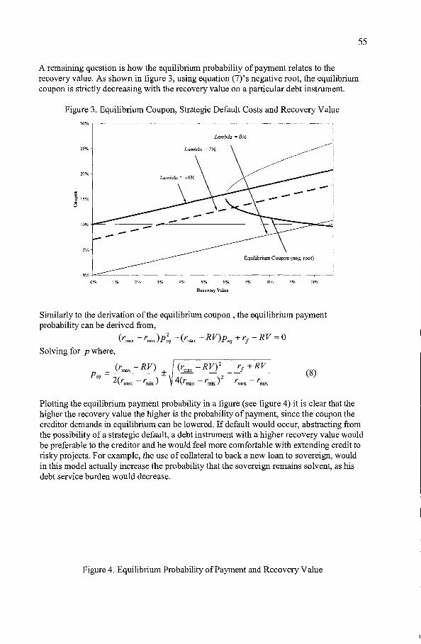
55

A remaining question is how the equilibrium probability of payment relates to therecovery value. As shown in figure 3, using equation (7)'s negative root, the equilibriunlcoupon is strictly decreasing with the recovery value on a particular debt instrument.

Figure 3. Equilibrium Coupon, Strategic Default Costs and Recovery Value

30% .,.............--------------------------........-....-,

Lambda = 0%

20'%

=Q§' 15'%

U

5%,

Equilibrium Coupon (neg. root)

0% -t-=---,--------.--,.--------r------,----.-----,-----...---.----r-------'

o'y., 1%1 2(% 3'% 4'% 6'y.,

Recovery Value

7(){, 8% 10%

Similarly to the derivation of the equilibrium coupon, the equilibrium paymentprobability can be derived from,

(rmax - rrnin )p~q - (rmax - RV)Peq + rf - RV =0

Solving for p where,

(rmax - RV)Peq = ±

2(rmax - t;nil1)

(rmax - RV)2

4(rmax - rmil1 ) 2

(8)

Plotting the equilibriunl payment probability in a figure (see figure 4) it is clear that thehigher the recovery value the higher is the probability ofpayment, since the coupon thecreditor demands in equilibrium can be lowered. If default would occur, abstracting fronlthe possibility of a strategic default, a debt instrument with a higher recovery value wouldbe preferable to the creditor and he would feel more comfortable with extending credit torisky projects. For example, the use of collateral to back a new loan to sovereign, wouldin this nlodel actually increase the probability that the sovereign remains solvent, as hisdebt service burden would decrease.

Figure 4. Equilibrium Probability ofPayment and Recovery Value

Equilibrium Probability ofpayment,ifno strategic default

(positive root)

56

80%,

70'%

60%,

50%i:it!

~40%,

g~

30%,

eCl.o

20%

10%,

0%.

0%

-10'%

1'% 2% 3% 4%1 6%1

Recovery Value

7'% 8% 9% 10%

F. Effect on Secondary Market Price of Already Existing Debt

While the equilibriums derived and discussed above reflect the effects ofchanges in keyvariables on newly contracted debt, already existing debt will also post significant pricechanges with changes in RV and A. If for example the debt instrument underconsideration is near the strategic default frontier and the cost of default is reduced, thatparticular debt instrument would see its price fall from its par value to its recovery value(RV ), despite that the fundamental repayment probability of the sovereign remainsunchanged.

In the case of changes in RV ,it would affect the price of the debt instrument by re­arranging equation (3) to,

p = E(15 t+l ) = p(rp > c)(l + c)D + (1- p(rp > c»(l + RVo + i1RV)D

t (1+rj ) (1+rj )

where RVo represents the old equilibrium recovery value and MV the change in

recovery value. The impact on the price of the existing debt instrument by changing therecovery value can then be simply expressed as,

M =_(l_-_p_(r_p _>_c_))_M_V(1 + rf )

(9)

with a positive price change if the recovery value increases and a negative price change (aloss to the creditor) if the recovery value is reduced.

57

G. Implications

When considering recent initiatives to enhance PSI in crisis resolution, it could beworthwhile to consider how these initiatives affect the debt instrument specific recoveryvalue and cost of default. For creditors, being able to discipline debtors is therefore acrucial aspect of international debt flows. If the cost of default is lowered, there may bean effect on the availability and structure of the future financing provided by creditors,i.e., they will adapt. Moreover, it would cause sharp price falls for those debt instrumentsand debtors, for which the cost of default frontier was binding.

As figure 2 shows, the decision on whether, for example, to make a debt contract easier torestructure, and hence reduce the cost of default, depends on whether the cost of default isalready seen as too high and hence a reduction would on net reduce welfare losses, or ifthe cost of default is in an intermediate area, in the above example between 0 and 10percent, where it is binding and actually reduces the amount ofrisky lending. A reductionin the cost of default in this case would reduce the lending to risky borrowers, while lessrisky debtors would be unaffected by small enough changes in the cost of default.

Moreover, if default costs are very high, only countries that suffer from extreme bad luckand are in very bad shape will default. By definition this means that the average recoveryvalue for all creditors will be very low. If, on the other hand, default costs are low, suchthat debtors with plenty of spare debt servicing resources choose to default, recoveryvalues for a while will be higher, as the debtor and creditor can agree on a debt serviceprofile that could be serviced at a higher level than in the case of a truly bankrupt debtordefaulting. An implication, therefore, from the framework presented here is that ifenhanced PSI in crisis resolution means the net lowering of the costs of default, andlending occurs with the cost of default in the intermediate area, recovery values followingdefault should be expected to go up and not down.

It should also be noted at the outset that if creditor moral hazard plays an important rolein world capital markets it will also affect the key parameters for the debtor. Multilateralfinancing packages that include no private sector involvement, and hence maintaincreditor moral hazard in the system, will lower the cost of default for the country (bymitigating output losses), lower the probability of default (an up-front lower interest canbe charged by the creditor as he has some "insurance"), and increases the recovery valueif default still occurs. Therefore, initiatives that increase the cost of default and reduce therecovery value, may be optimal in a world where the level and structure of financingflows has already been impacted by creditor moral hazard. However, if the creditor moralhazard inherent in the global financial system is believed to be limited there is less roomto make the argument that the creditor's position needs to be weakened, as the currentstate most likely already reflects an equilibrium outcome with debtor moral hazard butlimited creditor moral hazard.

What the model therefore shows is that the balance between creditor and debtor "rights"is a subtle one and great care needs to be taken to not shift the balance too far in eitherdirection. Moreover, whether the current cost of default in the international capitalmarkets is in the intermediate area or too high, would critically determine whether effortsto reduce a debtor's default costs would increase or decrease welfare.

58

IV. EXTENDING THE MODEL: PRIVATE SECTOR ADAPTATION

In the simple model introduced in the previous section, there is little scope for the privatesector to adapt, i.e. change fronl an easier to restructure debt instrument to one that isharder to restructure. Rather the private sector creditor's decision is a simple one, to lendor not to lend and at what price. Drawing on recent experiences, the later sections willargue that private sector creditors have shown, or will show, a remarkable ability to adaptto changed circumstances if the perceived cost of default incurred by a sovereign debtorchanges. To put the below discussion on a somewhat firmer footing the previous section'smodel is expanded to include two fonns of debt, e.g., sovereign bonds and sovereignloans. A key outconle of the nl0del extension is that the inlportance of the, for someunattractive, key assumption of strategic defaults, i.e. that a country would not be willingto pay in some states of the world, even though it is able to, can be relaxed. Instead, theassumption is replaced by that in some states of the world a sovereign debtor may nothave enough resources to service both types of debt. Hence, it would have to choose,which type of debt to service. Clearly, if one type of debt is inherently costlier torestructure, the debtor is less willing to default on that particular debt instrument and willcontinue to service it as long as it is able to.

A. Model Extension

Consider, the model introduced in section II, but now assume that a sovereign debtor canfinance the project through both loans, share of r, and bonds, share of 1-r.An investorwill in equilibrium, taking into the probability of default on the bond, charge a coupon ofCB , while a bank would charge a coupon of CL • Furthermore, it is assumed that both

bonds and loans have the same recovery value (RV) for the creditors, but the cost ofdefaults (AB and AL ) are different for the two instruments. Reflecting the comnlon beliefin the market, and in the absence of embedded collective action clauses in dollar­denominated (New York law) sovereign bond issues, AB is typically larger than AL •

However, the cost of default both in terms of AB , AL and RV is a function of the amount

defaulted on, i.e. related to r46. As a result of the above assumptions, the probability of

paying the two debt instruments would affect the sovereign's utility function in equation(2) in the following way:

U~ == p(rp > rCL + (l-r)c B )[rp -rcL -(I-y)cB]+

[rp -n'(YCL +(I-r)(RV +AB)) ]

+ p(rcL + (1- r)cB > rp > rCL) ,-(I-II )(1- r)cB + r(RV + AL)) (10)

+ p(rcL > rp > (1- r)CB)~p - r(RV + AL) - (1- r)cB]

+ p«I- r)cB > rp)[rp - r(RV + AL) - (1- r)(RV + AB )]

46 This assumption is the same as in Eichengreen, Kletzer, and Mody (2003). See thisreference for a more detailed discussion of the trade-offs related to the choice of howdefault costs relate to the amount of debt defaulted upon.

59

As can be seen in equation (10), the probabilities implicitly assumes that rCL > (1- r)cB ,

i.e. the weighted coupon payments are higher on the loans than on the bonds. This wouldhold as long as:

Cy> __B_ (11)cL+cB

The second line of equation (10) reflects the choice a sovereign would face betweenpaying either the loan or the bond, when it lacks the resources to service both (note this isquite different then assun1ing that a country would strategically default on all debt).Similar to the original model, the choice is reflected by a dummy variable II', which isequal to 1 if the sovereign decides to default on the loan first, which it would do if thefollowing expression holds:

rp -r(RV +AL)-(I-r)cB >rp -YCL -(I-r)(RV +AB ) i.e.,

r> cB-RV-AB RB (12)cL -RV -AL +cB -RV -As RL +RB

Equation (12) states that if the share of loans held by the sovereign exceeds the relativereturn from defaulting on the bond (the sovereign would save RB ifit defaults on thebond) divided by the total return from defaulting on both bonds and loans equallyweighted, a sovereign would default on the loan before defaulting on the bond47

. Hence,since RL > RB , i.e. the return from defaulting on the loan is in equilibrium always largerthan the return from defaulting on the bond, since a loan creditor has to protect himselffrom the lower cost of default by charging a higher coupon (if the ratio is less then 0.5).Therefore, if the share of loans is fairly large it is more attractive for the sovereign todefault on the loan first and the bond second (as long as the weighted coupon payments ofthe loans are higher than on the bonds). Assuming that the inequality in equation (11)holds, reflecting that the initial share of loans in a sovereign's debt is significant, theprobabilities for the default on bonds and loans can be derived and the full utility functionbe presented. Assun1ing the same uniform probability distribution for rp as in the basic

model, the probabilities are:

( (1) )- rmax - rcL - (1 - y)cB

p rp > rCL + - Y cB -rmax - rmin

rc - (1- y)cp(rcL + (1- r)cB > rp > rCL) = L B

rmax - rmin

(1- r)c - rp(rcL > rp > (1- r)cB ) = B min

rmax - rmin

p«(1- r)CB

> rp

) = (1- r)CB

rmax - rmin

47 Similar to the basic model it is assumed that RL and RB are larger than zero.

60

By substituting these probabilities into the sovereign debtor's revised utility function andmaximizing with respect to the share of loans chosen, i.e. r, the below expression isderived:

r = rmin(AB -AL)-rmax(cB -CL)+cB (2RB -RL) (13)

2(CL RL + 2cB (RB - RL ))

To maximize his utility a sovereign debtor will choose a r (share of loans) that ispositively related to the attractiveness of the project (the larger the differencermax - rmin the larger the probability that the return will exceed the coupon for any constant

coupon and rmin > 0) and the coupon a debtor has to pay for the bond, i.e. the higher thebond coupon the n10re a debtor will use loan financing.

The key objective of this model extension is to explore the relationship between the shareof loans held by a sovereign and the cost of default on bonds (AB ). It was in1plicitlyargued in the introduction that due to private sector adaptation if the cost of default onbonds is reduced there will be relatively less den1and for bonds and more for loans. In themodel extension this relationship can be evaluated by taking the partial derivative of rwith respect to the cost of default on bonds, i.e.,

(14)

which can be shown to be negative, i.e., a~A.B < 0, as long as y <1-Y,';i'CB

(the

partial derivative threshold) and the share of loans is below the ratio expressed inequation (12) 48. Hence, even this simple n10del extension shows that the share of loans,i.e. the sovereign borrower's adaptation to a change, strictly increases with an increase inthe cost of default on bonds.

B. Numerical Example

Expanding on the numerical example of earlier sections, assume that the sovereign canchoose between bond financing and loan financing. Keeping the coupon ofbonds andloans both constant (assun1e cB = 10% and cL = 13%), a recovery value of2.5 percent, a

cost of default on the loans of 0 percent, and rmax and rmin as before, equation (13) would

evolve as suggested in figure 5.

48 Please note that it is assumed that the relative coupon payments on loans are higher thanon bonds, and that the debtor would default on loans first. Reversing the last assumptionwould still yield a similar expression and the same conclusions. The partial derivative

would, however, be negative as long as y' < 1- r~CB •

61

Figure 5. The Share of Loans in Optinlunl and the Cost ofDefault on Bonds100% ..--------..---.----- -.---.--.- ---------.----..-.---.-.-.-- ---.-- ---- - ----..-. 100%

80%

60%e

!0- 40% ......

" ....= .... .. ......= " ....3 20%~

jrI)

0%

80%

60%

40%

-20%• • • Default return ratio

- Part. Derivative threshold

- Share ofLoans ifDefault on Loan first

-20%

-40% -40%

0.1% 1.1% 2.1% 3.1% 4.1% 5.1% 6.1% 7.1% 8.1% 9.1%

Cost of Default on Bonds

As expected, and as long as the share of loans in optimum is below the partial derivativethreshold, the share of loans will be declining as the cost of default on bonds increases.This is a non-linear relationship reflecting that the bonds become increasingly attractiveto the sovereign debtor (as well as the private creditor, especially ifwe allow the couponpaid on the bonds to adjust when the probability of default is reduced) as the cost ofdefault on bonds increases. If the cost of default ofbonds decreases, the impact on theshare of loans is clearly positive, as the two instrunlents become more similar. However,how much the share of loans would increase depends on how large the cost ofdefault onbonds was initially. If it was quite large (above 9 percent in the example) the impactwould be quite significant, but if it was small, the share of loans would hardly change.Note that in this example, the loan and bond coupon is kept constant and the defaultprobabilities as well. Hence, since the sovereign would find it more attractive to firstdefault on the loan (and the coupon is constant) it will prefer the loan to the bond evenwhen the cost of default on the bond is similar to that on the loan, i.e. the share of loan isat its highest 70 percent rather than 50 percent. In the next section, the model findingswill be used to put into context the ongoing policy discussion relating to sovereign crisisprevention and resolution.

v. DEBT PAYMENT SUSPENSIONS: PRIVATE SECTOR REACTION AND AnAPTATION

During a financial crisis the capital outflows from a country may be so overwhelming andbroad-based, reducing the country's foreign exchange reserves, that there is no time toenter into negotiations on how to restructure the debt, and a suspension on debt paymentsand other capital transactions, including the freezing of domestic bank deposits, may haveto be announced. While the outflows can originate in the corporate sector, a nlassiveoutflow may lead to the socialization of the debt in order to salvage the local financialsystem as well as avoiding the wholesale bankruptcy of a country's corporate sector. Insuch a situation a sovereign will be faced with the decision, which debt payments hewishes to suspend first, a pecking order of debt, and for what amount of time. As

62

discussed in the previous section, this default decision will depend on the relative costs ofdefaulting on some debts and not others. Moreover, the sovereign needs to consider; howcomprehensive should the suspension be; which asset classes will be affected (e.g. bonds,loans, equity, don1estic or external, etc.); will the suspension be voluntary or coercive; isit intended to be done with the implicit sanctioning of the official community; and whatare the implications of the suspension for future market access. Therefore, the coverageand n1agnitude of debt payments suspended can vary between delaying one payment onParis Club debt, leaving the external private sector debt intact, to the full scale impositionof capital controls, declaration of a corporate and sovereign standstill and the freezing ofbank deposits. The private sector creditors will react and adapt to all these decisions forwhich debt payments are suspended, both ex-ante and ex-post.

Unilateral suspensions of domestic or foreign debt payments form a natural, but unwantedpart, of all debt restructuring. They are and have been a fact of life for debt instruments.Frequently, the actual time it takes for a sovereign or a corporate to launch a restructuringoffer for either its bonds or loans, means it may have to actually enter default and riskcollateral damage doing so, before a successful restructuring has been completed.Collateral damage could in this case result in an inability to borrow internationally anddomestically, the trigger cross-default clauses with the debtor losing control over the debtrestructuring process, a grab race for assets prompting a fire sale, loss of investor anddomestic confidence, collapse in the secondary market value of the debt, disruptivelitigation and a broad-based rush to the exit triggering large capital outflows by bothdomestics and foreigners. These potential side effects of entering into default, bydeclaring a unilateral suspensions, have led a number of observers both in the official andacademic community (See Eichengreen, 2000 and Miller and Zhang, 2000 for overviews)to suggest a more predictable framework to manage suspensions, taking as an examplethe US corporate bankruptcy context. There have been many suggestions.49 Some ofthem are: the setting up of an international bankruptcy court replicating US chapter 11protection for sovereign debtors; giving the IMF the right to declare a stay on litigationand declare temporary payment suspensions; or to officially, explicitly or implicitly,sanction debt payment suspensions by allowing the IMF to lend into private sectorarrears.

While all of these proposals take the current state ofplay with potentially damaging ad­hoc payment suspensions as given, few of the recent studies consider that for some typesof creditors, as noted in the literature overview, there is an advantage ofhaving anunpredictable and uncontrolled payment suspension procedure in place, as it increases thedebtor's cost of default. Furthermore, few observers have considered what is the potentialimpact on the structure and level of international capital in a world where the officialsector is increasingly willing to sanction debt payment suspensions.5o As indicated in themodeling section, a more orderly framework for payment suspensions may have a similareffect on private sector adaptation, as that of reducing the cost of default in figure 2.Whether a more orderly framework will be welfare increasing or welfare reducing clearlydepends on whether one believes that the current cost of default imposed on debtors is

49 See IMF (2000b) for a brief overview.

50 Some exceptions are IMF(2000a) and IMF (2000b).

63

beyond the range where more risky projects can receive new financing if the cost ofdefault is increased. Hence, the actual experience to date is analyzed in more detail next.

A. Issues Regarding Orderly Payment Suspensions

The advantage ofpayment suspensions for the debtor in crisis, at least in theory, is thatthey can lock in both foreign and domestic private sector capital in a given country for alimited time period by restricting net capital outflows. Fron1 the official community'spoint of view the n1ain policy challenge has been viewed as being whether and howpayment suspensions should be officially sanctioned and whether a predictableframework for their imposition is needed. There are several variables that will affect theimpact ofmore frequent payment suspensions:

Can Payment Suspensions be Voluntary?

It is likely that payment suspensions will have the least effect on the future structure ofinternational capital flows if they are voluntary, i.e., forbearance by a certain creditorgroup in return for some "sweetener". The inherent problem with the voluntary approachis that it is similar to raising new money. If a country only suffers from a temporary debtservice hump and asks some creditors to forego debt service payments during that humpin order for a larger debt service payn1ent later, the debtor could instead issue a new bondrather than declare a payment suspension for a certain creditor. Hence, sovereign debtorswill not declare a payment suspension in cases where they are facing a pure liquidityproblem, as raising new debt is a realistic option and a better choice. There would be, forexample, no reputationalloss or risk that the debtor opens himself up to litigation threatsetc.

If market access has been lost, and a payment suspension may be the only option, it ishard to see how it can be completely voluntary. At a minimum there is at least a need fora credible threat of default to encourage some creditors to agree to a payment suspension.In a situation when solvency concerns are in1portant as well as liquidity concerns, thevalue a debtor can offer a creditor in a voluntary payment suspension negotiation wouldbe through arbitrarily making that creditor's claim de facto senior to that of othercreditors.51 Hence, the sweetener needed to reach a voluntary agreement with one creditorgroup will in this scenario occur at the expense of another creditor group. However, thisis analogous to either issuing secured debt or very short-term debt. Voluntary paymentsuspensions also allow for the asymmetric treatment of creditors with limited potentialran1ifications down the road. Partially-voluntary, or coercive payment suspensions mayhave to be comprehensive across all, at least, foreign currency creditors, whetherdomestic or senior, in order to avoid the creation of new seniority structures.

51 For example, in return for its forbearance, a creditor will either receive ancillarybusiness if it is a bank, or have its claim's obligor status be upgraded to that of thesovereign rather than that of a corporate (see for example the description of the Koreancrisis experience in IMF (2000a)).

64

Coordination Problem?

In the cross-border enlerging corporate borrowing context voluntary payment suspensionshave been quite common for both bonded debt and syndicated lending. The presence of awell-established bankruptcy procedure and creditor protection, in order to avoid assetstripping, makes voluntary payment suspensions more credible and easier to negotiate. Inthe sovereign context there is no bankruptcy court and it is therefore natural to expect thatvoluntary payment suspensions will be harder and costlier to negotiate. The direct costs ofreaching a payment suspension agreement with a group of creditors will both depend onthe maturity of their clainls and how other creditors are being dealt with.

• Longer-term creditors will be unwilling to agree to a payment suspension if theirforbearance is being used to bailout shorter-term creditors. Unlike the 1980s wherethe long-term and short-term creditors were the same group ofbanks and could bemore easily coordinated, the current creditor dispersion will make coordination muchharder. Moreover, the very nature of the causes of the crisis will have an effect on thefeasibility of reaching a payment suspension agreement. For example, longer-termcreditors may be more willing to accept a pause in debt service if they believe that thepause will be used to enact reforms that increase the likelihood ofbetter debt serviceperformance in the future. However, to agree, these longer-term creditors will ask forsome sort of sweetener. The attractiveness of the sweetener, however, will be afunction ofwhether the country is illiquid or insolvent, i.e., depend on the magnitudeof the creditor concession required. In cases where the size of the sweetenerdemanded by creditors to agree to a voluntary payment suspension is larger than thecountry's medium-term debt servicing capacity, a voluntary payment suspensioncould not be arranged unless it is expected that the "residual", the gap between thesweetener and the debt service capacity not covered, is supplied by a third party, forexanlple the official comnlunity.

• Furthermore, the size of the sweetener is likely to be affected by thecomprehensiveness of the payment suspension. If only long-term investors are askedto participate, for the implicit benefit of the short-term investor, then the sweetenerwill most likely be upsized to reflect this.

• Shorter-term creditors will be costlier to convince to participate voh,mtarily in apayment suspension. In situations where this group of investor is fairly small, theywill face the decision of either running now and receive the full par value of theirclaims, or running later and either receiving a recovery value (because there exists apossibility that the sovereign will be in default even after the agreed to paymentsuspension period ends) or the par value plus sonle sweetener. Hence, short-termcreditors could potentially agree to a payment suspension if the sweetener is largeenough, and contrary to longer-term creditors, the present value of the sweeteneroffered has to exceed the par value of the short term credit.

What if Payment Suspensions are Not Voluntary?

Partially voluntary or coerced non-comprehensive payment suspensions are more likely tohave an impact on the future structure and level of international debt flows, since, bydefinition, various groups of creditors are more or less likely to be amenable to moralsuasion or coordination. If, for example, one group of creditors is more likely to be

65

successfully subject to moral suasion and hence convinced to participate in a paymentsuspension for a non-voluntary sweetener, that creditor group is likely to adapt and in thefuture make sure to reduce its vulnerability by either charging a higher fee up front, i.e.,incorporating the moral suasion risk in its initial lending decision, or reduce the amountof capital it actually lends and thereby its exposure (similar to the analysis behind figure2). Hence, a partially voluntary payment suspension may be successful in resolving oneparticular crisis, but may soon loose its usefulness as an instrument, since credit flows arelikely to be increasingly channeled through the creditor groups that are less amenable tomoral suasion.

In a worst-ease-scenario, where a sovereign debtor is insolvent, and broad based capitalflight is occurring, the debtor may have no other choice than to resort to declare aunilateral payment suspension in this exceptional case. Extending the scope ofpaymentsuspensions to most private creditor groups as well as freezing, in this example, bankdeposits, may both give some breathing space to the sovereign debtor as well as avoidingan asymmetric treatment of creditors. Thus, making the payment suspensioncomprehensive would close all potential capital outflow channels and treat all privatecreditors symnletrically. By not favoring one asset class over another, this approach linlitsthe incentives for the private creditors affected by the payment suspension to create seniordebt further down the road.

Should Some Private Creditors be Treated as Senior?

Arguments have been made that some private sector creditors should receive preferentialtreatment when a payment suspension is imposed. Notably this discussion has focused ontrade credits or new money extended to the sovereign during a crisis. However, theexperience of the 1980s provides some useful examples on how the private sector willadapt if certain debts are treated preferentially. The example ofthe 1980s restructuringexperiences' impact on sovereign syndicated lending was already mentioned above.Another lesson from the 1980s was the fact that in many cases trade financing wasexcluded from loan renegotiations and hence creditors and debtors had a natural incentiveto structure future general purpose credits in the form of trade credits (see Buchheit,1991). With respect to new money the motivation for treating them as senior is often saidto be that it is in all creditors' interest to make sure that the country can still get access tocapital in order to limit the output losses that occur during the crisis. This is notnecessarily true. As mentioned in the modeling section, output losses may be the onlyeffective disciplining device creditors have available to ensure re-payment. New moneyshifts the bargaining strength somewhat towards the debtor. Hence, it is not clear whetherall private creditors necessarily favor the approach ofmaking new money senior.52

B. Payment Suspensions and the Composition of Cross-Border Debt Flows

As mentioned above partially voluntary or coercive payment suspensions that are notcomprehensive, i.e., one creditor group is treated more favorably than another, are verylikely to lead to a change in the composition and level of debt financing flows to

52 See for example the heated discussion on this issue in the context of the SDRM debate,for example, Roubini and Setser, 2003.

66

emerging markets in the future. While this prinlarily impacts the recovery value ofaffected debt instruments, some have argued that a benefit ofmore frequent impositionand official sanctioning ofpaynlent suspensions is that it would make short-term debt lessattractive and long term debt more attractive. This line of reasoning assunles that theincentives of longer maturity debt are more similar to those of the sovereign debtor aswell as those of the official community. For example, temporary paynlent suspensions ononly short term debt could perhaps still allow the sovereign to service its long term debt.Unfortunately, however, when a country starts moving towards a crisis situation thematurity of its debt stock will most likely shorten because:

• Foreign creditors will almost by definition be unwilling to take long-term exposuretowards the country as previously long-term debt falls due.

• This unwillingness by foreign creditors to extend new long-term credit will lead to anupward sloping yield curve, making long-term borrowing for the country very costly.This would encourage a shift by the debtor to borrow through shorter-terminstruments. As creditors increasingly offer shorter-term loans at increasingly higherinterest rates, the yield curve of the sovereign is likely to widen out as well as flatten.Eventually, when a debt service interruption becomes imminent, the yield curve of thesovereign debtor will invert, with markets pricing in a very high risk of default in theSh011 end.

• A payment suspension on debt amortizations, where the sovereign still makes interestpayments, may lead to default on longer-term bonds or loans that are amortizing or tothe non-payment ofprincipal of initially long-term debt that matures within thepayment suspension period. In such cases, the payment suspension could triggercross-default clauses on other longer-term debt as well. Longer-term creditors willthen have to decide whether they want to accelerate their debt and be treated similarlyto the short-term creditors in the resolution, or if they want to keep their accelerationoption open as long as their debt is still being serviced. Shorter-term creditors mayalso demand, as a condition to agree to a restructuring, that longer-term creditors arebrought to the negotiation table.

c. Implications

If officially sanctioned, the resulting higher likelihood of a payment suspension, andthereby the reduction in both the cost of default and perhaps also the recovery value, mayencourage a shift in the maturity structure of debt toward the shorter end of the spectrum,as creditors move to protect themselves. This can be done, for example, by providingfinancing only in the overnight market, to ensure a withdrawal before a paymentsuspension becomes operational. Hence, if the main benefit ofhaving nlore orderly andofficially sanctioned payment suspensions is to reduce the reliance on short-tenn debt, itis worth noting that it may create the reverse result, encouraging creditors to lend at evenshorter maturities to ensure that they get their money out. Indeed, one interpretation of the1980s debt crisis resolution is that a similar dynamic was at work when bank lendingshifted, following the resolution of the crisis, from mainly medium- and long- termnlaturities to short term interbank debt. Maturities shorter than that of interbank lineswould severely restrict the ability of a paynlent suspension from being effective. In thenext section, the experience with sovereign bond restructurings are analyzed.

67

VI. BOND EXCHANGES AND PRIVATE SECTOR ADAPTATION

Facing a situation where a payment suspension, whether con1prehensive or not, lookslikely, a sovereign debtor could try to approach its bondholders to discuss reprofiling thebond payments to avoid the actual imposition of a payment suspension and a subsequentdefault. As discussed before, truly voluntary agreements will be uncommon as trueliquidity crisis situations will be hard to distinguish from solvency ones and the outcomeof any bond restructuring or reprofiling discussion after market access has been lost willbe determined by the credibility of the sovereign's default threat. During the few yearsthere have been defaults on both sovereign eurobonds as well as Brady bonds53 and bondexchanges ofdefaulted or nearly defaulted bonds have been completed by Pakistan,Ukraine, Ecuador and Russia.54

The ease and success of the recent bond exchanges have surprised many. The reason forthe surprise was that eurobonds and Brady bonds were believed to be technically hard torestructure both for legal reasons (for example, requiring unanimity and due to the threatof litigation) and for practical reasons (for example, the identification and coordination ofthousands ofbondholders). It may be too early to draw conclusions about the applicabilityof recent bond exchanges for future bond restructurings, however, because the cost ofdefault, A, may have been lower than expected and creditors will seek new forms of debtinstruments with a higher A and/or RV , shifting emerging market borrowing andlending decisions to a new equilibrium where financing may be reduced or more costly.Moreover, the impact on already issued bonds will also reflect a certain adaptation to thenew circumstances of lower or higher A or RV . For example,

• Private creditors will adjust upwards their price at which they are willing toparticipate in future bond exchange if recent experience is viewed as indicating thatemerging market bond recovery value estimates were too low. As shown in equation(9) a higher RV would increase the price of existing debt making it harder to offerlarge sweeteners (arguably what is currently a key concern in Argentina's ongoingnegotiations with its private sector creditors currently). For future lending decisions ahigher recovery value will according to the model reduce in equilibrium theprobability of default, for the same debtor, and would be beneficial for both debtorsand creditors, as more risky sovereign debtors would receive financing.

• While the success of recent bond exchanges has put into question creditors' cost ofdefault estimates, i.e., the cost of default may be lower than previously anticipated, amore broad based introduction of collective action clauses or the use of exit

53 As several authors have pointed out, for example Eichengreen (1999) and Petas andRahman (1999), defaults on international bonds have been frequent historically speaking,especially in the 1930s. In 1999, Ecuador was the first sovereign to default on botheurobonds and Brady bonds. Subsequently, there have been sovereign bond defaults inIvory Coast and Argentina. Uruguay's recent distressed sovereign debt swap was clearlycon1pleted against a credible default threat and involved significant NPV losses forprivate creditors.

54 As discussed in IMF (2000a).

68

amendments may reduce the cost of default even further. However, recent successfullitigation (e.g. Elliot and Peru), could indicate that the threat of litigation has perhapsalso been underestimated and may actually make bond exchanges more costly in thefuture and work in the opposite direction to the initiatives ofmaking bonded debteasier to restructure. Again Argentina's success or failure on this front, given itsaggressiveness towards all its creditors, could settle this debate.

• Private creditors are likely to adapt the structure of their lending vehicles in ways suchthat restructuring and creditor coordination nlay be more difficult in the future. Asargued in the model extension, sovereign loans could also increase in importance, asthe relative advantage bonds face is gradually eroded.

In the next sub-section the impact on existing sovereign bondholders of the recentexperiences of easier than expected bond exchanges will be discussed. Changes inrecovery value and cost ofdefault estimates by these bondholders will have a key bearingon whether bond restructurings will be as easy to complete in the future. Following thisdiscussion and using the basic model as a background, the second subsection will discussthe impact ofboth collective action clauses, exit amendments and the renewed litigationthreat on both existing bonds and the future lendinglborrowing equilibrium. The lastsubsection will go further towards reflecting over how the bondholders could adapt in anew equilibrium by changing the structure or terms of their lending.

A. Impact on Outstanding Bonds and Bond Restructurings

In evaluating bond exchanges, different investor groups will have different reactionfunctions. Mark-to-market investors, having borne the full brunt of the fall in secondarymarket price of the to-be-exchanged bonds, tend generally to compare the NPV value ofthe exchange offered (at some discount rate) to the current market price of the to-be­exchanged bonds and with the recovery value of not participating in the exchange. In thesimplest case, if the NPV of the exchange bond is higher, taking into account the

.likelihood of the exchange succeeding and the haircut in temlS of a potential debt write­off, then the holder of the to-be-exchanged bond has an incentive to tender his bonds inthe exchange. This is the way most fund managers would rationally respond. Forcommercial banks a sinli1ar response function is less likely, as they generally do notmark-to-market all of their investment portfolios, but a reasonable approximation. Theresponse function of retail investors is much more uncertain as their tender decision maybe based less on a NPV comparison then on whether or not they have to participate in adebt write-off.

Market Reactions to Recent Bond Exchanges

(in percent)

Price 1-Price 1- week Price 1- Face

Date or Exchange Exchange Listing dayafier before week after Priceal value Completion / Post-ancmnt/ Completion / pre·Detault Announced Completed Price default ancrnnl ancnml completion wrile-o!l' listing price pre-ancmntprice ancmntprice

Pakistan

6% USD 2002 eurobond no Delaull 11/15/99 12/6/99 100.0 58.3 60.4 63.6 -36

Ukraine16%DEM 2001 eurobond 1/20/00 2/4/00 4/7/00 100.0 50.0 55.5 67.0 81.5 -19 21 47

RussiaPrins 12/2/98 2/11/00 8/17/00 57.8 6.5 18.5 24.4 32.0 -38 -45 32 73fans 6/2/99 2/11100 8/17/00 67.2 10.0 21.1 25.0 32.8 -33 -51 19 55

EcuadorBrady Par Bond 11/28/99 7/27/00 8/11/00 27.4 35.8 35.5 39.5 39.5 -60 44 11 11Brady Discount Bond 8/28/99 7/27/00 8/11/00 47.0 34.4 37.0 46.7 46.7 -42 -1 26 26Brady PDf Bond 2/28/00 7/27/00 8/11/00 27.0 23.5 25.3 30.5 30.5 -22 13 21 21

NOle: Bonds presented are not all ofthose resuuctured. Prices are ask and includes accrued interest., when bond is in delilUlt For Pakistan accrued interest is estimated.

Delault is the date oflhe lirst missed coupon payment., except in the case ofUkraine. where the delault rellects the missed amortization on its Ocl-2000 eurobond.

69

The recent successful bond exchanges have involved some fOIDl of sweetener (see tableabove). For example, the post-announcenlent price has been 10-30 percent higher than thepre-announcement price, with the exception ofPakistan. In Russia, the sweetener wasenhanced with the upgrade in the obligor to that of the sovereign. Large sweeteners havein many cases also reduced the incentive, for at least mark-to-market bondholders, tolitigate, since capturing the sweetener provides an inmlediate gain while the outcomefrom litigation is tIDcertain and tinle consuming.

The limited experience to date with external bond exchanges, required that several keyparameters of the debt pricing equation presented in equation (3) and the cost of defaultwere "guesstimated". For example, the recovery value had without much empirical basisconsistently been estimated at 18-20 cents on the dollar for sovereign eurobonds. lftherecovery value is actually much higher, for example close to the average recovery valuein the US high-yield sector (47 cents on the dollar with an average 2.1 years forcollection55), market prices ofbonds that were in default would shoot up, as reflected inequation (9), to reflect the new revised estimate of recovery values. It may be that lowrecovery value estimates were one reason why prices post-announcement could crediblybe substantially higher than prices pre-announcement in all the recent bond exchangeswith the exception ofPakistan. In Pakistan, however, the actual number ofbondholderswere limited and fairly well known in advance and the high share of locally connectedinvestors reduced the necessary size of the sweetener.

In addition to the size of the sweetener, enhancing recovery values further is the speed ofcuring the default (this would also reduce the cost ofdefault to the debtor, so the neteffect in equilibrium may be ambiguous). The experience from recent bond exchangessuggest that they were completed much faster-than-expected (1-2 years compared to thelost decade of the 1980's debt restructurings), and in one case the exchange was evencompleted before the actual default occurred (Pakistan). Bond exchanges are, however,not guaranteed to succeed and significant deal risk may remain even after they arealU1ounced, but overall the probabilities of success for the recent exchanges onceannounced have been very high,56 partly reflecting the large mark-to-market gainsinherent in the offers for tendering bondholders (again see table).

Recent exchanges, such as the one in Ecuador and Ukraine, have taken a "carrot" and"stick" approach to encourage bondholders to tender into the exchange. The adaptation ofprivate creditors' expectations of recovery will make it more difficult to offer similarcarrots (i.e., large mark-to-market gains) in the future. For example, if the recovery valuefollowing default is now believed to be consistently higher than before, secondary market

55 Rappoport (2000) and Rappoport and Xu (2000) for a much more detailed discussionon the sensitivity of emerging market and U.S. high-yield bonds to default probability,recovery value and other assumptions.

56 This can be determined by looking at the differential between the price of the newexchange bond when-issued (basically forward contracts on the new bond) and the priceof the old to-be-exchanged bond. A small differential implies that investors believe theexchange will succeed. When-Issued markets existed in all the four bond exchanges.

70

prices will actually not fall as low as they did, for example in the Russian case, and henceoffering as attractive a sweetener may not be credible from a debt-service capacity pointofview. Therefore, it remains to be seen whether the experience with recent bondexchanges are useful in deternlining whether future bond exchanges will be equallysuccessful. These bond exchanges have, however, managed to very successfully addresssonle of the issues with regards to the technical aspects ofhow to restructure sovereignbonds that were unknown before. By doing so, these exchanges have firmly pierced the"halo" that was previously believed to surround eurobonds and Brady bonds. It remains tobe seen whether the private sector adapts by switching into harder to restructure lendinginstruments.

B. Cost of Default, Legal Innovations and the Threat of Litigation

The recent bond exchanges by Ecuador, Pakistan, Russia and Ukraine are generallyregarded as successful in terms of having obtained a high degree of investor participationwhile avoiding creditor litigation. The keys to success of the voluntary exchanges havebeen the sweeteners provided. As discussed above, when the market adjusts itsexpectations for recovery values it will become more difficult to offer such sweeteners inthe future and the threat of litigation may increase. The experience of recent bondexchanges and their success, together with the official community initiatives to increasethe prevalence of collective action clauses57 (CACs) raise the question whether theseevents have an impact on the cost of default and how it will affect the future emergingmarket borrowing/lending equilibrium.

Collective Action Clauses and Exit Consents

As discussed in IMF (2000a) the actual usefulness of CACs in bond exchanges to datehas been limited.58 For example, it appears to have been less difficult than anticipated to

57 The clauses, commonly referred to as CACs are: a majority action clause (allowing aqualified majority ofbondholders to bind a minority); a sharing clause (stating that anyfunds received through, for example, litigation by one bondholder, have to be shared withthe other bondholders based on their share of the outstanding bond); and a collectiverepresentation clause (allowing a trustee, for example, to represent bondholders,facilitating majority actions). CACs can facilitate creditor-debtor negotiations, since theyreduce both the threshold needed for achieving a restructuring agreement (the majorityaction clause) and the potential threat of litigation from "holdout" creditors (reducingtheir incentive to litigate through the sharing clause). Bonds issued under English lawtypically include CACs. These clauses are not regularly contained in bonds issued underNew York law.

58 Enlpirical work, however, suggests collective action clauses tend to reduce the cost ofborrowing for some borrowers. See for exanlple, Eichengreen and Mody (1999), and for amore critical assessment Becker, Richards and Thaicharoen (2000). Recent experience ofissuing dollar-denominated New York law eurobonds has had mixed results. As discussedby Eichengreen, Kletzer, and Mody (2003), the experience to date with Mexico's andBrazil's CAe bond issues have indicated some secondary market premium (related to thereduced cost of default), but it remains to be seen ifit will be sustained, and perhapsreturn when a country with CACs again approaches a sovereign debt crisis.

71

organize and locate individual bondholders and to offer them an exchange. Moreover, thevalue of CACs as a threat to encourage bondholders to tender in an exchange seen1Ssecondary. As discussed earlier, it was the large carrot (sweetener) that clinched theexchange deals rather than the stick. However, there is at least one example of CACsbeing used as a stick. Ukraine dealt with potential holdout creditors within the context ofits voluntary exchange offer by making use of the CACs embedded in three of the fouraffected bonds, after a substantial majority had agreed to the exchange. Experience wouldtherefore suggest that the main usefulness of CACs is that they effectively limit litigation,while exit consents59 (introduced for the first time in Ecuador's bond exchange, seeappendix 1, 2. Gertner and Scharfstein (1991) discuss exit consents in the US corporatecontext) can be used to increase the success and ease of any bond restructuring.

However, the more widespread use ofboth CACs and exit consents have the potential ofreducing the cost of default for the debtor, increasing the possibility of a strategic default,with a subsequent shift in the lendinglborrowing equilibrium (from A to B in figure 2).Again, similarly to the discussion n1ade in the payments suspension section, the actualoutcome on the level of financing flows will depend on whether the preceding cost ofdefault was binding or not. For example, if creditor moral hazard is ignored, and if thecost of default would be binding, and allow for the maximum of amount of financing toemerging market sovereign in equilibrium (in figure 2 this would be consistent with aA=10 percent) any reduction in the cost of default would lead to a reduction in financingavailable to more risky emerging market sovereigns thereby reducing welfare. As morethan 60 percent of the J.P. Morgan EMBI+ benchmark index is compromised by issuersbelow investment grade it is likely that these are also the debtors most sensitive tochanges in the cost of default. The impact on flows to emerging markets could besubstantial. Note, however, that this effect, according to the simple model would notshow up in the spreads or coupons the debtors have to pay. If strategic default isbecon1ing increasing likely for a debtor, no creditor would extend financing at anyrealistic interest rate. Moreover, higher-quality debtors would be unaffected. In terms ofempirical evidence, see IMF (2000c) there are some evidence that currently bondfinancing to emerging market sovereigns remain ample, and only the lowest, for examplesingle-B minus creditors, are facing some rationing in the market.

The Litigation Threat

One of the major deterrents to creditor litigation has been the difficulty of attachingsovereign assets. First, many assets can quickly be hidden if the sovereign believes themto be at risk. Second, US case law suggests it may be difficult to attach significant assetseven in the case of a favorable ruling. However, the prevailing belief that litigation

59 The use of exit consents is a strategy that, similarly to CACs, can be employed toprovide the stick in a bond exchange and induce bondholders to participate in theexchange by changing key non-payment terms and thereby reducing the value of the oldbond after the exchange has been con1pleted. The main advantage of exit consents is thatthey can be used in bonds that otherwise would require unanimity to change any of theirpayment terms, and they can thereby replicate some of the features of CACs. Exitconsents in a sovereign NY-law bond were first used in Ecuador. See Buchheit & Gulati(2000) for a very insightful discussion.

72

remained a rather limited threat, may change because of the recent success ofElliottAssociates in its case against Peru (see appendix 3).

If sovereign litigation as an alternative becomes feasible and economical for creditors,they will have a further tool to counteract any reduction in the cost of default.Surprisingly, as visible in figure 2, the subsequent increase in the cost of default may forsome parameter values be welfare enhancing. Some litigation may therefore be a goodthing, depending on what the overall cost of default is, and may put a limit to other formsof creditor adaptation, by changing the form of the lending instrument.

C. Changing the Structure of the Eurobond Market

In the same way creditors adapted to the restructuring experiences of the 1980s bychanging the structure of their lending vehicles through increasing the cost of default orreducing their lending by charging a higher interest rate up front, following the recentbond exchanges, there may be incentives for private sector creditors to again adapt insuch a way to avoid the shift to a low financing equilibrium (point B in figure 2).Increasing the seniority of the lending instruments, by increasing A or RV , also has avalue to avoid default or to have an improved claim in a restructuring situation. A creditorcan increase the seniority ofhis claim in a nunlber of ways, either through requesting up­front collateral, private or public sector guarantees or changing the ownership and votingstructure of the creditor (nlany more are possible):

• As mentioned in the introduction, there may be an increased demand among creditorsfor lending vehicles that are collateralized by the borrower with cash flows or realassets that can be captured outside the debtor country's borders and hence couldeasily be transferred into the control of the creditors in the event of a default. The twomain types of collateral that a sovereign could pledge would be its foreign exchangereserves or future export revenues60 of its state-owned companies, such as oil ortelecom. By definition the amount of collateral available to be easily pledged limitsthe use of collateralized borrowing for the debtor. While there is a significant amountof quasi-sovereign collateralized bonds outstanding, to date none of thesecollateralized bonds have been restructured. Specifically, it is uncertain how onewould actually go about restructuring these bonds and ask the creditor to take asignificant haircut. In the case ofPakistan, one eurobond that was not involved in therestructuring was a governn1ent guaranteed Pakistani Telecom bond, which wascollateralized by the future export earnings on incon1ing international telephone calls.According to Standard & Poor's (S&P 1999) the structure of the Pakistani Telecombond showed the resiliencies ofthese types of transactions and ifdefault would occurrecovery values will be very high as creditors can access the collateral, which isusually placed in an off-shore trust.

60 Rating agencies assign future flow securitizations substantially higher ratings (up tofour notches in some cases, see S&P, 1999) as the political and transfer risk of these typesof debt are mitigated by their structure. In emerging markets, major examples of issuersusing future flow securitizations are PdVSA and PEMEX (Venezuela's and Mexico's oilcompanies).

73

• An alternative would be lending guaranteed by either official or private insuranceentities. For example, by making its lending conditional on the presence of a WorldBank "policy-based guarantee" a lender should be able to make himselfmore immuneto risks of unwanted PSI. Argentina, for example, issued policy-based-guaranteebonds in October 1999 and Colombia is considering raising part of its financing in2001 through the use of such World Bank guaranteed bonds. Other public guaranteeprogrammes such as the IFC's B-Ioan program, and that of other IFIs, effectivelyextend the preferred creditor status of these institutions to private creditors. In suchcases, it is unclear how these bonds would be restructured. After the experience ofArgentina default, where some of these bonds were restructured regardless of theguarantee, the attractiveness of IFI backed instruments have decreased.

• The use of collateralized borrowing is largely limited to corporations and could berelevant to the sovereign in the case of large export oriented state-owned companies,which the sovereign can use for its borrowing purposes. Hence, there would beincentives to find additional ways of lending money where the security from trying toavoid PSI stems from how the lending transaction is structured. It would, for example,be possible to repackage bonds and loans through the use of collateralized-bond­obligations (CBOs) or collateralized-loan-obligations (CLOs) and separate the legalownership of the debt instrument, and hence the power to vote to participate in a debtexchange, from the stream ofpayments accruing, in such a way that it would beextremely difficult to find a representative of the actual creditor lender with the rightto decide on participation in the exchange on behalf of the CBO/CLO. The point isnot that it would be impossible to restructure a CBO and CLO, but that it is moredifficult, adding to the cost of default for the debtor ifhe decided to default on debtinstruments which are predominantly held by CBOs and CLOs.

The above are some of the potential adaptations that bondholders could opt for. Thesimplest one is of course to increase the borrowing cost for the debtor. However, it maybe in both the creditors' and sovereign debtors' interests to race up the seniority ladder inorder for more debtors to find cheaper financing and for the creditors to protectthemselves. It is unclear whether such a seniority race is in the interest of officialcreditors, both bilateral and multilateral.

VII. IMPLICATIONS AND CONCLUSIONS

Efforts at crisis resolution that succeed in reducing potential inefficiencies and instabilityin the international financial system are in the interest ofboth the private and the publicsector. In the absence of clearly established rules of the ganle, the approaches adoptedtoward crisis resolution, and the extent to which they are interpreted by marketparticipants as setting a precedent, can have profound implications for the workings of theinternational financial system and the nature and structure of international capital flows.

A key lesson from the 1980s is that as particular lending instruments are involved in-restructurings, the private sector will seek out new instruments that increase theprobability of repayment and are insulated from restructurings. The large-scalerestructuring of syndicated bank loans in the aftermath ofthe 1980s debt crisis, whileleaving eurobonds untouched, provided an important impetus to the use of theinternational bond market for emerging market borrowers. The experience with concertedinterbank rollovers in Korea, Indonesia, and Brazil have shed some light on how the

74

private sector will adapt to an increase in the frequency ofpayment suspensions. Theexpectation by the market that this will be the case will likely lead at least someinternational banks to cut their lines and run early in the face of an imminent crisis.

Experience following the most recent string of crises has firmly pierced the halosurrounding international bonds. This experience with bond restructurings will likely leadbondholders to update their estimates ofkey variables, such as the cost of default and therecovery value, making recently successful bond exchanges less useful as predictors ofthe success or failure of future bond exchanges. A key question about the welfare effectsof recent official sector crisis resolution initiatives is whether the current cost of default istoo high, and welfare can be gained by reducing it, or it is in the intermediate regionwhere a reduction would lead to a loss in welfare. Moreover, it is natural to expect that, asbond restructurings become more common, private sector creditors will increasingly tryto structure debt such that it is harder to restructure, for example, by issuing securitized orguaranteed debt or adopting investor holding structures that are difficult to negotiate with.

Such private sector adaptation to official sector crisis resolution initiatives, as discussedabove, may not be costless and will either lead to increased borrowing costs for the debtoror to more short tenn and rigid debt structures, as the sovereign debtor tries to offsetincreases in borrowing costs by agreeing to borrow through ever more advanced andrenegotiation proof structures. Either way, the net effect on emerging market capital flowmay be negative, especially for the lowest quality sovereign borrowers.

The ongoing sovereign debt restructuring in Argentina is probably the event that willdetermine the direction for international debt lending to emerging nlarkets and the threatof litigation for years to come. An unduly messy outcome, which looks increasinglylikely given delays, will again raise calls for the intervention by the official community toresolve perceived market failures. Perhaps, even the recently shelved SDRM proposalwill be dusted off. If this happens, this chapter hopefully can serve a role in cautioningreinvigorated policy makers to keep private sector adaptation in nlind and revisit whetherthe main problem is too low sovereign default costs or too high.

75

APPENDIX 1. OVERVIEW OF THE ECUADOR BOND EXCHANGE61

On September 28, 1999, Ecuador became the first sovereign to default on a Brady bondafter the expiration of a 30-day grace period. It can be argued that the crisis had been longin the making and reflected internal political problems aggravated by external shocks,such as the "El Nifio" weather phenomenon. At the time of the default Ecuador's externalbonded debt consisted of collateralized Bradys (Pars and Discounts) with an outstandingamount of$3.1 billion, uncollateralized Brady (Past-Due-Interest, PDIs) amounting to$2.8 billion and a stock of $0.5 billion of dollar-denominated eurobonds.

Figure A.l. Ecuador: Debt Service Profile2.6 - ..----...- ...---.--...-.----.--••---.-•....-.---..•- .•...--.--..-..•-----.-.------.-----.-..-------•..--..-.. 2.6

2.4

2.2

=o:s~ 1.8VJ::J=

1.6

1.4

1.2

2000 2001 2002 2003 2004 2005 2006 2007 2008 2009 2010 2011 2012

2.4

2.2

1.8

1.6

1.4

1.2

Sources: Markel estimates. I- Before Restructuring - - After I

In July, 2000, the authorities launched its exchange offer, offering to exchange thedefaulted bonds for about $4 bn in new bonds and about $1 bn in cash (accrued interestand principal collateral). Sinlilar to Russia, the exchange offer involved a significant debtwrite-off (haircut relative to Par) of 40.6% even exceeding that ofRussia (which gave asa sweetener an upgrade in obligor). Some bondholders could choose between exchangingtheir defaulted bonds into, either an amortizing 30-year eurobond with a step-up couponfrom 4% to 10% or, to a certain extent, an amortizing 12-year eurobond with a 12%coupon in return for an extra 35% haircut. In contrast to the principal collateral, interestcollateral was used to pay accrued interest. As one ofmany interesting features, theexchange offer discriminated between Brady bonds and the shorter-term eurobonds,where no initial debt write-offwas asked for. Moreover, eurobonds did have a priority inswitching to the 12-year eurobond. This option was designed as being valuable and a capwas set for the 2012 issue size implying that none of the Par and Discount holders wouldreceive the shorter-maturity bond. The PDI bond, reflecting relative historical price

61 Updates description of the Ecuador exchange in IMF(2000a), for the description ofother exchanges please see IMF(2000a).

76

performance, was treated differently compared to other uncollateralized Brady debt (theIEs) and eurobonds, which were not initially subject to a debt write-off.

In the end, approximately 97% ofbondholders accepted the exchange offer partly due tothe cash sweeteners but also because of the use of exit amendments discussed in appendix3. While many investment banks continue to question Ecuador's debt sustainability (seeRoubini, 2000), the exchange did provide some breathing space for the sovereign. Debtservice payments are, however, expected to come back to pre-exchange levels by 2005.

77

APPENDIX 2. INNOVATIONS IN THE ECUADOR BOND EXCHANGE62

The Ecuador bond exchange included many innovations, conlpared to the other bondexchanges, in order to make the exchange successful for bonds that were subject to NY­law. Especially challenging was the question ofhow the sovereign could limit thepotential of future litigious activity from any potential hold-out creditors and encouragelarge majority ofbondholders to tender. The solution proved to be a clever use ofcashsweeteners (see appendix 1), exit consents, and principal reinstatement clauses.

Exit ConsentsThe exchange offer is the first example of the use of "exit consent" amendments in asovereign bond context (a "poisoning the well behind you" strategy) to make it lessattractive for hold-out creditors to remain in the old bond and not tender. Such changes tonon-payment terms of the old bonds only required a 51 %-75% majority of agreeingbondholders, while any change of the payment terms, under NY-law, would haverequired unanimity. Tendering bondholders agreed to when "exiting" the old bond to:strip away cross-default and cross-acceleration provisions to the new bonds (the newbonds include a cros~-acceleration clause but it cannot be triggered by continued defaultson the old bonds); reduce liquidity of the old bonds by delisting them; change negativepledge clauses; limit attachment possibilities of debt service made on the new bond; andmore. In addition, Ecuador changed clauses in the old bonds allowing it to not extinguishtendered bonds ifnecessary, such that hold-outs cannot reverse exit amendments andcannot accelerate the old bonds.

Principal ReinstatementAs an additional sweetener to those investors who received the 2030 exchange bond inreturn for the Brady Par, Discount and PDI bonds (37% of PDT bondholders did notreceive any 2012 eurobonds) the bond documentation included a principal reinstatementfeature, which in the event of default would reinflate the principal by up to 30 percentagepoints (if default occurred in years 1-3, 20 percentage points if it occurred in years 4-6and 10 percentage points if it occurred in years 7-10) and thereby mitigate some of thehaircut relative to par imposed on the tendering bondholders today (Par 60%, Discount42% and PDT 22%). Given the significant default probability of Ecuadorian eurobondsfollowing the exchange the reinstatement feature did provide some value (a marketestimate put the value of this feature at about 11% of the market price of the 2030eurobond in August), but is based on the belief that any future restructuring will be basedon the nominal value of the defaulted bonds rather than the market value or some othermeasure.

62 References for this appendix is Buchheit and Gulati (2000) and Lindenbaum and Duran(2000).

78

ApPENDIX 3. BACKGROUND ON ELLIOTT ASSOCIATES VERSUS PERU63

On Friday the 29th of September 2000, Peru announced it would pay Elliott Associates(Elliott) in full its $58.4 million claim, in order for the sovereign to make a $80 millioncoupon payment overdue on some of its Brady bonds (with the grace period expiringOctober 7). Against a backdrop of domestic turbulence, more than three years of legalproceedings, and with restraining orders having been served to the paying agent as well asseveral other banks and the two major clearing houses, Peru had no credible alternativebut to pay Elliott.

Elliott, a well-known distressed debt investor and having won a similar case with respectto Pananla, initially bought during early 1995 $20.7 million in nominal value sovereignguaranteed defaulted bank loans and paid $11.7 million. The purchase decision followeda favorable court decision involving another distressed debt investor, Pravin Banker, anda Peruvian ban1e After deciding not to participate in Peru's Brady deal of October 1996Elliott decided to immediately go to court in order to try to attach paynlents that werebeing transferred fronl Peru to the New York Fed in order to purchase the collateralnecessary for the Brady deal. This strategy failed and several years of legal challengesfollowed. On October 20th 1999, and after a ruling by a lower court, which had dismissedElliott's claim that its purchase of Peruvian debt had not been "with the intent and solepurpose to sue", a US appeals court on ruled in favor of Elliott and reversed the lowercourt's decision. Legally, Elliott effectively managed to revoke the use of the"Champerty" doctrine defense64, making it easier for future distressed debt investors (i.e.vulture funds) and other creditors to sue a government and attempt to attach its assets.

On June 22nd, 2000, Elliott was awarded a judgment order against Peru and could start

seeking to attach assets. The September 7 coupon payment was the first payment after thejudgment and Elliott sought and was granted restraining orders for the fiscal agent Chaseas well as for several other banks and Buroclear and Cedel (after having received afavorable restraining order judgnlent from a Belgian Appeals court). For the sovereign, atthis point, time ran out before it could challenge the restraining orders and it paid Elliotton October 4, 2000. All-in-all Elliott made profits of $46.7 million, minus legal fees, orabout a 400% on its original investment 4.5 year earlier.

Lindenbaum and Duran (2000) draw the following lessons from the Elliott case:

• "Champerty offers little protection for sovereign debtors, supporting the perceptionthat a ruling in favor of creditors is relatively easy to obtain."

63 This appendix is based on several of the legal documents surrounding the case as wellas a summary analysis by Lindenbaum and Duran (2000).

64 Under section 489 of the New York Judicial law a creditor is forbidden to acquire debt"with the intent and for the purpose ofbringing and action or proceeding thereon", seeLindenbaum and Duran (2000).

79

• "The threat of attaching bond coupons is credible." Ecuador's exchange bonds are,however, trying to protect themselves from some aspects of the Elliott risk. Notably,Ecuador uses a Trustee (creditor' s agent) rather than a fiscal agent (debtor' s agent)making any transfers to the trustee the property of the creditor rather than that of thedebtor, making attachment more difficult.

• "Sovereigns are unlikely to be able to bypass orders of attachment in the location ofthe fiscal agent by paying coupons via a branch office, especially on existing bonds."

In the end, the applicability of the Elliott versus Peru case will not be clear until othercreditors follow in Elliott's footsteps and clarify some of the outstanding legalambiguities that are outside the scope of this chapter to discuss. It is fair to say, however,that the case has led to increased investor interest into the legal details of their debtcontracts.

80

REFERENCES

Becker, Torbjorn, Anthony Richards, and Yunyong Thaicharoen, 2.000, "CollectiveAction Clauses for En1erging Markets Borrowers: Good News for Lower RatedBorrowers Too," (Washington, IMF, mimeo).

Bolton, Patrick, and David Scharfstein, 1996, "Optin1al Debt Structure and the Number ofCreditors" Journal ofPoliticaI Economy, Vol. 104 (no. 1), pp. 1-25.

Bolton, Patrick, and David Skeel, 2003, "Inside the Black Box: How Should a SovereignBankruptcy Framework be Structured," mimeo, (April, unpublished).

Buchheit, Lee, 1991, "The pari passu clause sub specie aeternitatis," InternationalFinancial Law Review (December).

---, 2000, "Sovereign Debtors and their Bondholders," Vnitar Training Programmeson Foreign Economic Relations, Docun1ent No. 1 (Geneva: Unitar).

---, and G. Mitu Gulati, 2000, "Exit Consents in Sovereign Bond Exchanges," UCLALaw Review, Vol. 48 (October), pp. 59-84.

Bulow, Jeremy, and Kenneth Rogoff, 1989a, "A Constant Recontracting Model ofSovereign Debt," Journal ofPolitical Economy, Vol. 97 (February), pp. 155-178.

---, 1989b, "Sovereign Debt: Is to Forgive to Forget?," American Economic Review,Vol. 79 (March), pp. 43-50.

Chui, Michael, Prasanna Gai, and Andrew Haldane, 2000, "Sovereign Liquidity Crises:Analytics and In1plications for Public Policy," working paper, (London: Bank ofEngland).

Cline, William, 1995, "International Debt Reexamined," Institute for InternationalEconomics (Washington: lIE, February).

---, 2000, "The Role of the Private Sector in Resolving Financial Crises in EmergingMarkets", Institute of International Finance (Washington: lIP, October), mimeo.

Dooley, Michael P., 1994, " A Retrospective on the Debt Crisis," NBER Working PaperNo. 4963 (Cambridge, Massachusetts: National Bureau of Economic Research).

---, 2000, "Can Output Losses Following International Financial Crises beAvoided?" NBER Working Paper No. 7531 (Cambridge, Massachusetts: NationalBureau of Economic Research).

Eaton, Jonathan, and Mark Gersovitz, 1981, "Debt with Potential Repudiation:Theoretical and Empirical Analysis," Review ofEconomic Studies, Vol. 48(April), pp. 289-309.

---, and Joseph Stiglitz, 1986, "The Pure Theory of Country Risk," EuropeanEconomic Review, Vol. 30 (June), pp. 481-513.

81

Eichengreen, Barry, 1999, "Toward a New International Financial Architecture: APractical Post-Asia Agenda" (Washington: Institute for International Economics).

---, 2000, "Can the Moral Hazard Caused by IMF Bailouts be Reduced," GenevaReports on the World Economy Special Report 1 (Geneva: International Centerfor Monetary and Banking Studies).

---, and Ashoka Mody, 2000, "Would Collective Action Clauses Raise BorrowingCosts?" NBER Working Paper No. 7458 (Cambridge, Massachusetts: NationalBureau ofEconomic Research).

Haldane, Andy, 1999, "Private Sector Involvement in Financial Crisis: Analytics andPublic Policy Approaches," Financial Stability Review, Bank ofEngland(London: November).

Gertner, Robert and David Scharfstein, 1991, "A Theory ofWorkouts and the Effects ofReorganization Law, " Journal ofFinance, Vol. 46 (September), pp. 1189-1222.

International Monetary Fund, 2000a, International Capital Markets: Developments,Prospects, and Key Policy Issues, World Economic and Financial Surveys(Washington:IMF, September).

---, 2000b, "Involving the Private Sector in the Resolution ofFinancial Crises­Standstills - Preliminary Considerations," Policy Development and ReviewDepartment and Legal Department (Washington:IMF, September).

---, 2000c, "Emerging Market Financing: Quarterly Report 011 Developments andProspects," Research Department (Washington:IMF, November).

Lane, Timothy, and Steven Phillips, 2000, "Does IMF Financing Result in MoralHazard?", IMF Working Paper WP/OO/168 (Washington:IMF, October).

Lindenbaum, Eric, and Alicia Duran, 2000, "Debt Restructuring: Legal Considerations ­In1pact ofPeru's Legal Battle and Ecuador's Restructuring on Nigeria and OtherPotential Burden Sharing Cases," (New York: Merrill Lynch & Co., October).

Minovi, Maziar, and Jens Nystedt, 2003, "Sovereign Debt Restructuring: Facts andFiction," mimeo (Washington: IMF, July).

Morris, Stephen, and Hyun Song Shin, 1998, "Unique Equilibrium in a Model of Self­Fulfilling Currency Attacks," American Economic Review, Vol. 88 (June), pp.587-597.

Petas, Peter, and Rashique Rahman, 1999, "Sovereign Bonds-Legal Aspects that AffectDefault and Recovery," Global Emerging Markets-Debt Strategy (London:Deutsche Bank, May).

82

Prasanna Gai, Simon Hayes, and Hyun Song Shin, 2000, "The Role of Sovereign DebtStandstills in Crisis Management," working paper, (London: Bank of England,December).

Rappoport, Peter, 2000, "Valuing Credit Fundamentals: Rock-Bottom Spreads", (NewYork: J.P. Morgan Securities Inc., April).

---, and David Xu, 2000, "Emerging Markets versus High Yield: CreditFundamentals Revisited", (New York: J.P. Morgan Securities Inc., October).

Roubini, Nouriel, 2000, "Bail-In, Burden-Sharing, Private Sector Involvement (PSI) inCrisis Resolution and Constructive Engagenlent of the Private Sector. A Primer:Evolving Definitions, Doctrine, Practice and Case Law", mimeo, (New York,Stem School ofBusiness, New York University, unpublished).

---, and Brad Setser, 2003, "Improving the Sovereign Debt Retsructuring Process:Problems in Restructuring, Proposed Solutions, and a Roadmap for Reform,"mimeo, «New York, Stem School ofBusiness, New York University,unpublished)).

Standard & Poor's, "Lessons From the Past Apply to Future Securitizations in EmergingMarkets," (New York, Standard & Poor's, July).

Zettelmeyer, Jeromin, 2000, "Can Official Crisis Lending be Counter-productive in theShort-Run?, "Economic Notes, Vol. 29 (February), pp. 13-29.

---,2003, "How Can the Cost ofDebt Crises be Reduced?," mimeD, (Washington:IMF, unpublished).

83

Chapter III

European Equity Market Inte~ration:Cyclical or Structural? 5

I. INTRODUCTION

The interdependence between international financial markets have become increasinglyevident during the last several financial crises, TMT (technology, media, and telecom)bubble,. and European Monetary Union. Such integration has made it increasinglychallenging for portfolio managers to seek out diversification opportunities and has raisedthe question on whether traditional investment techniques such as country-based investingshould give way to global industry based investing. However, financial integration,loosely defined, can stenl from at least two different sources. First, and the one most oftenthought about, is a common investor base. International institutional investorsbenchmarked to certain global equity indices, such as the Morgan Stanley CapitalIntemational66 (MSCI) index family, own stocks in different countries and evaluate themrelative to a common benchmark. Such common ownership sets the stage for co­movements, especially in crises, as investors may be forced to liquidate positions to meetend-investor withdrawals. It thereby risks increasing the co-movement between differentcountries and sectors. A second potential source of increased financial integration is thedegree of internationalization of corporations. Multi-national corporations with largeoverseas sales can be as sensitive to overseas market developments as to developments intheir home market. In this latter context it would be reasonable to expect country factorsto slowly decrease and sector factors to gradually grow in importance in tune with long­run factors, such as the globalization of trade and service. This may be of particularrelevance in the European Monetary Union, where regulatory initiatives and equitymarket competitions has widely been seen as increasing equity market integration. In thecontext of increased global integration it would become increasingly costly for aninstitutional investor to retain the traditional home bias, given results in an under­representation of certain sectors relative to the global portfolio and hence reducesdiversification opportunities on top ofnot being diversified across countries.

65 I am grateful to Clas Bergstroem, Robin Brooks, Bankim Chadha, Peter Englund,Haizhou Huang, Subir Lall, and Richard Sweeney for comments. The author also wishesto thank senlinar participants at the European Economic Integration in Swedish Researchconference and the Department of Finance, Stockholm School of Economics. Mygratitude also to the Tore Browaldh foundation for sponsoring an earlier version of thispaper.

66 According to MSCI (w\vw.nlsci.com) 90 percent ofintemational equity assets in the U.S.are benclmlarked to MSCI indices. A similar dominance seems to hold in Asia, whilearound two-thirds ofEuropean fund managers use the index. Clearly, the creation ofinternational benchmarks to evaluate perfonnance has been one important supportingfactor to the increased internationalization of institutional investor portfolios.

84

The degree of equity market integration and the relative importance of country factorsrelative to sector factors have been debated in several papers throughout the latter part ofthe 1990s. A clear tendency towards increased equity market integration in the EuropeanUnion was identified. However, such developments were also observationally equivalentto the global Tech, Media, and Telecom (TMT) bubble, where investors sought out andtreated TMT companies largely the same regardless of location. The purpose of thischapter is to revisit and update the degree of equity nlarket integration67 anl0ng theEuropean Monetary Union (EMU) members using an improved and more intuitiveapproach compared to the recent literature and a nlore updated dataset. The methodologyused estimates various sector's sensitivities to country and global sector factors, and ishence immediately useful for traditional portfolio analysis, rather than the approachesused in some of the literature, which evaluate the share of the overall variance of a stockor a sector that can be explained by country and global sector factors. In addition, thechapter tries to detennine the roles played by the global bull market and structural factors,such as the introduction of the euro and the roles played by foreign international andEuropean institutional investor in explaining the increased integration observed in therecent literature. The main focus is on the equity markets in the European MonetaryUnion countries, but the chapter also explores whether the integration trends observed areexclusive to the EMU countries or are also reflective of developments in the broaderEuropean Union. The more recent data series captures changes in index methodology, themove to free-float indices, and whether or not only the tech, media and telecom (TMT)sectors saw a broad based increase in the degree of integration. Moreover, the chapterdescribes and discusses the how the more intuitive approach measuring equity marketintegration compares to alternatives in the literature.

Using both average correlations and cross-section time-varying "beta" analysis theempirical results show a sharp increase during the late nineties in the importance of sectorcompared to country factors. 68 The methodology used to estimate the time-varyingsensitivities solves for the specification errors present in some other papers and providesfor estimates of the sector and country sensitivities that are immediately translatable intorelevant portfolio management statistics for institutional investors. The observed increasein "so called" equity market integration predates (perhaps in anticipation of) theintroduction of the euro and shows a remarkably steady rise throughout 1999. In fact, justbefore the burst of the tech bubble in MarchlApri12000, sector factors within the EMUwere as important as individual country factors. However, continning the cyclical natureof the observed equity market integration, the bursting of the bubble led to a consistentrelative decline in the importance of sector factors. This argues that there still remainssubstantial scope for further structural equity market integration within the EMU and, toan extent, past high levels of integration was a cyclical phenomenon. Despite the burstingof the Tech and subsequent Telecom bubbles, sectors such as Energy and Telecom renlain

67 As argued by Danthine et al (2000) the integration of EMU candidate countries foreignexchange, bond, and money markets preceded the actual launch of the euro. The corecountries of a future EMU were already perfectly anticipated by early 1997 with no realuncertainty regarding additional candidates existing after January 1998.68 The reference to betas could potentially lead to some confusion compared to themeaning ofthe term in the asset pricing literature. In line with the relevant literature, asimilar terminology will still be used but it is important to note that what is actually meantis the sensitivity coefficient to country versus sector effects.

85

still in 2002 largely global industries. Surprisingly the chapter finds that the Tech sectornever played the role of a truly global sector. This likely reflects the clear dominance ofthe U.S. Tech sector relative to that of Europe and that the equity returns ofmany of thesmaller Tech firms in the U.S. are more driven by country specific fundamentals.

The structure of the chapter is as follows: The next section will provide a brief literaturereview of the different approaches taken to discuss the amorphous concepts of financialor equity market integration and places the empirical approach taken here in to context. Insection III, the roles and importance of the intenlational non-European and Europeaninstitutional investors are discussed together with the scope for further equity marketintegration stemming from the gradual rebalancing of their portfolios to decrease theircurrent home-bias. Section IV discusses the data used in the chapter for the empiricalsection. While section V discusses the use of an average correlation approach to estimatethe degree of equity market integration, section VI compares the nlethodology used byother recent papers to estimate time-varying sensitivities with that used in this chapter.The section also argues that the methodology developed avoids a fairly importantspecification errors problem, especially if sector data is used rather than individual finndata. In the next section, section VII, the robustness of the observed increase in equitymarket integration is evaluated regarding the choice of countries and time periods. Thechapter ends in section VIII with a brief summary, some conclusions, and a fewsuggestions for further research.

II. FINANCIAL MARKET INTEGRATION IN THE LITERATURE

Throughout the 1990s the academic literature has debated financial market integrationfrom both macroeconomics and financial economics perspectives. At least four broadstrands can be distinguished. First, international macroeconomics has studied interestparity conditions to test for integration ofmoney and bond markets, and analyzed thedegree of capital account liberalization in countries to help determine the degree ofintegration. The macro literature has also tlied to quantify the benefits to countriesthrough increased international financial integration, such as improving the globalallocation of capital and helping countries to better share risk and reduce consumptionvolatility (see Kose et ai, 2002, for an overview). This literature has highlighted thatincreased financial integration also increases countries' vulnerability to shocks, i.e.contagion, and has argued that developing countries in particular should avoidprematurely liberalizing their capital accounts to potentially destabilizing capital flows.

A second, more financial econonlics based strand, has taken a capital flows perspectiveon financial integration and has studied the behavior of international investors and theshare of their foreign asset holdings relative to what would be optimal in an optimizingportfolio context. These studies have consistently found strong evidence of a home bias,as documented by Tesar & Werner (1995), which is incompatible with financial marketintegration having run its full course even in developed markets. The reasons for thehome bias include transaction and informational costs and have generated a largeliterature of their own. Updating Tesar and Werner's estinlates, Warnock (2002) showsthat initial estinlates ofhome bias were probably upward biased, since foreign equityholdings data were underreported. He argues, however, that there still remains substantialscope for further financial integration driven by more optimal portfolio allocations. Forexample, Warnock notes that while 50 percent of equities in a world portfolio are n011-

86

U.S., the share of foreign equities held by U.S. investors has remained relatively stable at10-11 percent since the mid-nineties.

A third strand of the literature has based test of financial market integration on aninternational capital asset pricing model, see, for example, Bekaert and Harvey (1995) orCampbell et al (1997) for overviews.

The last strand is a modification of the third and uses various time-series techniques, suchas correlation, cointegration, VAR, or multi-period regression analysis, to study the time­varying nature of financial market integration. Advantages of these techniques are thatthey easily map into pragmatic considerations for fund managers that are used to CAPM­like frameworks to optimize their portfolio performance. Ayuso & Blanco (1999) has,however, questioned whether these techniques actually measure financial integration oronly financial linkages. Comparing standard time series measures of financial integrationacross countries wit4 the result of these measures if they are applied to the New Yorkstock exchange, the authors argue that fmding significant increases in financialintegration could simply reflect a few outliers, such as the 1987 stock crash. Hence,econometric results of integration do not necessarily show that the equity markets studiedare from an economic point ofview more integrated. While less relevant for a portfoliomanager, Ayuso & Blanco's critique is a useful caution and potentially relevant from apolicy perspective69

. -

The cross-market correlation based literature has been among the most straight forwardand have been much used to analyze issues related to stock market crashes and financialcontagion (see Forbes & Rigobon (2002) for a critical discussion of some pitfalls withthis analysis). Solnik, Boucrelle & Le Fur (1996) found in their study, for example, thatduring the last 37 years, the level of correlation between the world's major stock marketshas been increasing. The authors conclude that this indicates that the markets havebecome more financially integrated. Another interesting result was that even thoughcorrelations between key markets were low during normal times, they jumped up in timesof crisis. This is a major problem for an investor following a correlation and countrybased risk diversification strategy, since the expected diversification benefit is notrealized during crisis. Hence, what looked like a well-diversified portfolio frequently isnot. Solnik et al concludes that even though correlations have increased steadily, therestill exist significant benefits from international diversification. Applying correlationanalysis to the European Union countries in the run-up to monetary union, Beckers (1999)argued that the gradual increase in correlation between EU equity markets would beboosted by the removal of exchange rate risk. For active portfolio managers, however,Beckers argued that EMU would increase the challenges to add value and that tighterintegration would increase the overall risk of institutional investor portfolios asdiversification benefits are strongly eroded.

Another approach has been to use cointegration techniques to find long-run relationshipsbetween equity markets in different countries. These studies have been focused onanalyzing whether stock market linkages during normal times fundamentally change

69 The authors note that the policy implications of finding tighter cross-country linkagesdiffer significantly if these linkages are driven by greater information globalization ratherthan greater integration, since the former maybe far more automatic .

87

during a crisis or some other discreet event. Taylor & Tonks (1989) largely started theliterature with their analysis of the impact of the abolition of U.K. exchange controls onthe degree of integration between U.K. stock markets and other developed markets. Sincethen, a number ofpapers have dealt with the October 1987 stock market crash(Arshanapalli and Doukas (1993), Chan and Lai (1993), and Ma (1993». This fairlysuccessful empirical approach has often been used to determine the direction of causalityusing granger-type tests. Arshanapalli and Doukas, for example, found evidence that theU.S. stock nlarket had a considerable impact on stock markets in France, Germany, andthe U.K., but not the other way. Other studies also frequently found evidence of a numberof cointegration relationship between both developed and developing equity markets (seeMasih and Masih (1997) and Chen et al (2002) for an application to Latin Americanequity markets) and have highlighted the inlportance of the US equity markets in beingthe originator of nlany shocks that have subsequent ripple effects. Within Europe,cointegration studies frequently identified Granger-causality running in both directionsindicating a tight links between especially European Union equity markets (see Nystedt(2000) and Ahlgren and Antell (2002) for recent examples).

A robust alternative to analyze the gradual change in the importance of country factorsrelative to the industry sector factors was pioneered by Roll (1992). Using a limiteddataset, but an econometrical technique based on Fama & MacBeth's (1973) classicalmethod for testing asset pricing models, Roll argued that global industry factors couldexplain up to 40 percent of the variation in individual country equity indices. Such a highexplanatory power was seen as equivalent to a high degree of financial integration acrossdeveloped equity markets, since country specific factors, unrelated to the industrial make­up of a country, played a much smaller role than previously expected in the literature.

Following up on Roll, Heston and Rouwenhorst (1994) pointed out that Roll's datalimitations had led to an overestimation of sector effects and therefore the degree ofequity market integration. Using an indirect estinlation technique to identify separatecountry and sector factors and using firm level data from 12 European countries between1978 to 1992, Heston and Rouwenhorst found that the difference in industrial structureacross country could only explain around 1 percent of the variance of country excessreturns. Hence, country factors, it was argued even in Europe in the early 1990s, fardonlinated any industry effects. Heston and Rouwenhorst use of individual stock data andtheir econometrica! techniques were subsequently applied by a number ofother authorson a variety of tinle periods and with a wider set of countries (see, for example, Beckerset al (1996) or Griffin and Karolyi (1998». These studies generally confirmed Heston andRouwenhorst's findings, but with an important exception being Western Europe, where aclear trend towards increased financial integration through increased sector importancewas consistently documented.

The run-up to the introduction of the euro in January 1999 sparked a series ofnew studiesanalyzing the importance of sectors versus countries with a special application to WesternEurope. Using broadly the same methodology, but varying datasets, Rouwenhorst (1998),Cavaglia et al (2000), and Baca et al (2000) all found evidence of sector effects gainingin inlportance in the European Union. Baca et al showed that sector and country factorswere now of roughly equal importance raising an important issue whether or notinternational institutional investors should base their diversification strategy on developedcountry sectors rather than countries. Cavaglia et al (2000), for example, showed thatdiversification across industries generated more risk reduction than a similar country-

88

based diversification strategy. They, therefore, argued that home bias could be morecostly in a more financially integrated world. Using an unfortunate example, from an ex­post point ofview, Cavaglia et al (2000) demonstrated that an institutional investorinvesting predominantly in United Kingdom, which has a very small share of tech firms,would loose out both in a country and sector sense, compared to investors holding theglobal equity market portfolio where the tech sector played a more important role.

Using a different methodology, based on time-varying betas estimates from observabledata series, Urias et al (1998) confirmed the sharp increase in the importance of sectors inexplaining stock returns in the run-up to the euro. By early-1998 capitalization weightedsector and country betas were ofbroadly equal significance, with sector betas likely toincrease further looking ahead. As a result, Urias et al also argued that institutionalinvestors should adopt a more regional or pan-European investment approach goingforward. However, in sectors that are likely to be more dominated by country factors,such as defense, country analysis should not be discouraged.

The advent of the euro was seen as strengthening the argument of increased equity marketintegration in the European Monetary Union. Increasingly, investment banks andinstitutional investors structured their operations around a sector basis rather than acountry basis. The tech, media, and telecom (TMT) sectors were the darlings of investorsall over the world sparking large capital flows to emerging equity markets, where sectorconsiderations were still generally dominated by country factors. The surge in interest forTMT stocks regardless ofwhere they were located spurred tighter integration among awide series of different equity markets. A recent study by Brooks and Del Negro (2002)argued that much of the increase in equity market integration can at the global level beexplained by the bull market, but find that at a regional level within Europe there aresigns that increased financial integration reflects more structural factors, such as theintroduction of a common currency. More recent research has sought to update thetechnique used by this strand of the literature by introducing regime switching features,such as Catao & Timmerman (2003). The regime switching approach is successful inidentifying a high and a low volatility regime. As could be expected, sector factorsincrease in importance during times ofhigh volatility, possibly reflecting common globalshocks such the oil shock of the 1970s and the boom and bust of the TMT sector. Inaddition, Catao & Timmerman confiIm the findings of the earlier literature that industryfactors have increased in significance during the late 1990s. Another approach has been toexplain in more detail the role played by global factors on an individual firm level ratherthan on a sector level, since shocks to this factor affect multinationals differently, whichhave a large share of sales abroad, than corporates, which are focused mostly on adomestic market (Cavaglia et al (2001) and Brooks & Del Negro (2003». Brooks & DelNegro (2003), for example, find a significant relationship between fimls that operateinternationally and their sensitivity to global shocks and argue that part of the decline inimportance of country factors observed in the earlier literature reflects that firms havebecome increasingly international, especially in the 1990s. Therefore, the importance ofcOlmtry factors has decreased more for those countries that have a large share ofmultinational firms.

III. EUROLAND AND INTERNATIONAL INSTITUTIONAL INVESTORS

OECD (2001) defines the term institutional investor to include insurance companies,pension funds and other private investment funds, including nlutual funds. As shown in

89

table A.l, the growth of institutional investor assets under management has beenspectacular across the DECD with assets under management increasing from around 97percent of GDP or US$23 trillion in 1995 to more than 140 percent of GDP or US$36trillion in 1999. The average annual growth rate within the OECD during this period wasa spectacular 11 percent per year, palily reflecting the late nineties' bull market.Nonetheless, institutional investor assets remain fairly concentrated, with the UnitedStates, Japan, and the United Kingdom increasing their share of total GECD assets undermanagement from 75 percent in 1995 to 76 percent in 1999. Within the European Union,EMU member have generally a lower asset to GDP ratio than other European Unionmembers do. This largely reflects large differences in the degree ofboth pension reformsand liberalization of institutional investor regulation (see Lanoo (1996)). No noticeablechange can yet be detected in the data regarding any inlpact of the EMU on assets undermanagement. The surge in assets under management tapered of quite significantly in2000, reflecting the much more difficult market situation, and should have remained on adeclining trend during the past two years despite significant new inflows.

Table 1. Institutional Investor BreakdownInsurance Companies

1995 1999Pension Funds

1995 1999Investment Funds

1995 1999

European UnionEMUUnited Kingdom

JapanUnited States

50%52%45%70%29%

47%44%49%670/023%

22%13%42%19%43%

20%11%38%200/040%

28%35%13%11%28%

33%46%14%12%37%

Source: GECD (2001)

Akin to a chicken and egg problem, the countries with the largest market capitalizationrelative to GDP also show the largest relative importance of institutional investors (seetable A.2). This relationship has spurred regulators, especially in the European Union, tosee what could be done to spur further growth in the importance of institutional investors.The introduction of the euro is expected to playa direct role in increasing the importance,competition and diversification possibility ofEuroland based institutional investors. Atpresent, see table 1, 44 percent of EMU institutional investor assets are held by insurancecompanies, only 11 percent by pension funds, and the renlainder by investment funds.These shares have not changed dramatically after the first year of the euro and remainsubstantially different to the large role played by pension funds in the U.K. and U.S.

90

Table 2. Asset Restrictions on Pension Funds and Life InsurersPension Funds

Bonds and Foreign CurrencyEquities Loans Assets Matching Equities

Life InsurersBonds and Foreign

Loans AssetsCurrencyMatching

Germany Max 30% Max 20% 80% Max 30% Max 20% 800/0France Min 50% No Max 65% Max 20% NoItaly P P P 33% Max 20% Max 20% 80%

U.K. P P P No Max 20% No

Japan Max 30% Min 50% Max 30% Max 30% Max 30%U.S. P P P Max 20% Max 20%

Note: P indicates that the prudent man rule applies.Source: Davis and Steil (2001) and Adjaoute and Danthine (2002)

Institutional investors across the European Union remain subject to fairly tight investmentrestrictions. The 2001 Lamfalussy report identified a number of areas where thereremained significant scope to increase regulatory integration in the treatment ofinstitutional investors70. Such efforts would allow for increased cross-border competitionto manage assets within the EU. During 2002, significant progress was reached regardinga "single passport" for pension funds and an EU wide use of the "prudent man rule"instead of the investment restrictions currently in place (see table 2). While both reformsare important, a wider use of the prudent man rule, after a transition period whereinvestment restrictions are gradually relaxed, could lead to a substantial increase in bothcross-border and equity investment. However, since many of these restrictions, seem notto have been binding, change is likely to be gradual rather than rapid. For example, asshown in table 3, foreign asset holdings by German pension funds were far below theregulatory maxin1um and while more updated data is not yet available, the investmentrestrictions are unlikely to be currently binding.

70 For a critical discussion of securities and market regulation in the aftermath of theLamfalussy report see Niemeyer (2001).

91

Table 3. Institutional Investor Investment in Foreign AssetsPension Funds Insurance Companies

1994 1998 1994 1998Mutual Funds

1994 1998

EDEMU

Austria 20%Belgium 350/0France 5% 5% 0% 0% 140/0Germany 6% 7% 0% 29%Italy 5% 0% 0% 0%Netherlands 17% 6%Spain 5%

OtherDenmark 7% 5%Sweden 12%U.K. 30% 18% 15% 13% 33%

Japan 7% 18% 9% 22%U.S. 100/0 11% 1%

Source: Lannoo (1996), Davis (1996), and Davis and Steil (2001)

As the equity bull market took hold equity holdings by Euroland institutional investorsshowed some increase towards the latter half of the nineties. A sharper increase (seefigure 1) occurred in 1999, after the introduction of the euro, reflecting both the decreasein currency risk to diversify to other markets, but also the outperformance of stocks inmany institutional investor portfolios. The high share invested by U.K. based institutionalinvestors under their prudent man rules is without comparison in the GEeD. While itunlikely, and perhaps not desirable, that equity investments by Euroland institutionalinvestors would reach such levels as seen in the United Kingdom,71 it is worthwhile tonote that a reallocation of their portfolios to the level invested by US institutionalinvestors could generate additional investment into the equity markets ofnearly US$150billion.

71 hl the context of the broad based equity market decline, since March/April 2000, theshare of equity investment by U.K. institutional investors should have declinedsignificantly. However, data that is more recent is currently unavailable.

92

Figure 1. Institutional Investors: Share Invested in Equities80% ...,..--------------------------,- 80%

70% --------------------------- 70%

60%

50%

40%

30%

20%

10%

--""",,--- ......

60%

50%

40%

30%

20%

10%

0% -I----..----.-----------r---r----.--------r----r-----..----+ 0%

1992 1993 1994 1995 1996 1997 1998 1999 2000Source: OECD: 2001

There renlains, therefore, significant scope for further investments in to the equitymarkets by both European based and other institutional investors. Such investments couldset the stage for further equity market integration both within the EMU and betweenregions. As seen in table A.2, European equity markets account for broadly 25 percent ofthe world equity market capitalization. Only 10-20 percent ofU.S. and Japanese pensionfund assets are invested abroad, implying significant future potential for foreigninstitutional investor interest in EMU equity markets. Of course, some of these inflowscould be offset by the rebalancing ofEMU based institutional investors to include morenon-euroland assets. Given the smaller asset base ofEuroland institutional investors andits concentration among more conservative insurance companies, US or Japanese inflowsare likely to in the medium-ternl more than offset European portfolio outflows.

Another factor arguing that there remains significant scope for further investor-ledfinancial integration is the predicted sharp growth in assets managed by benchmarkedEuropean institutional investors. Most EU countries have yet to adopt significant pensionreforms. De Ryck (1998), for example, estimates that between 1998 and 2008 pensionfund assets will increase ten times. This increase is seen as a natural reply to thedemographic developments in the EU countries and the need to create a funded andcredible pension system. Moreover, pension funds are in general long term investors,which should make it possible for them to increase the share of assets held in the form ofequities once the current bear market is deemed to have bottomed. Hence, Euroland-basedinsurance companies and pension funds are likely to playa very important role inincreasing the level of integration between European equity markets in the future,especially if recent regulatory initiatives to create a level regulatory playing field acrossthe European Union is indeed enacted.

IV. DATA

The data used for the subsequent sections analyzing the average correlation of sectors andcountries and time-varying sensitivities are based on Dow Jones World Stock dollar-

93

denominated Sector and Country Indices and market values (DJWI, see also Griffin andKarolyi (1998), who use the same index provider). Coverage starts in January 1992 andby December 2002 DJWI included 2,362 stocks in 22 developed countries, representingapproximately 95 percent ofboth European stock market capitalization and that of othercountries. In terms of sectors, DJWI divides stocks into 10 global sectors, 66 industriesand an additional 45 sub-industries. For the purpose of this chapter, daily data starting inJanuary 1996 and ending in April 2002 is used (a total of 1,646 observations by sectorand country).

Country coverage focuses nahrrally on the European Union and the US (see tables A.3and A.4) and has been further limited to those countries that have indices in at least threeout of the ten global sectors. As a result, smaller European countries such as Portugal,Greece, Luxembourg, Belgium, Ireland and Austria, have been excluded because of theirlack ofconsistent sector coverage. The excluded markets account for no more than 5percent of European Union market capitalization (see table A.2) or less than 1 percent ofglobal equity markets.

The choice between using dollar or local currency indices has been much debated in theliterature, and suffice to say the choice depends on what is the objective of the study.Given the focus of this chapter on institutional investors, the choice ofusing dollar returnreflects a pragnlatic consideration that most institutional investors are benchmarkedagainst a dollar-denominated version of an equity index such as the MSCI or DJWI.Therefore, as also argued by Davis and Steil (2001), many investment funds and someother institutional investors do generally not hedge their equity investments72

• None of thefindings presented below change materially if local currency indices are used. Moreover,in the run-up to the introduction of the euro, as noted earlier, EMU candidate currencieswere already very much aligned, as investors had anticipated the currency union throughconvergence plays in both foreign exchange and bond markets.

v. AVERAGE SECTOR AND COUNTRY CORRELATIONS

Correlation studies are probably the most intuitive way to analyze equity marketintegration (see for example Beckers (1996)). In addition to their simplicity, correlationstudies have an immediate link to optimal portfolio conlposition theory and is easilyunderstood and useful for portfolio managers. Studying the time-varying nature of thecorrelation between two stock indices or other financial assets has also frequently beenused by studies analyzing contagion during financial crises (see Forbes and Rigobon(2002)). Using some of the methods discussed in the financial contagion literature (seeIMF (2001)), the relative importance of sector effects compared to country effects areshown by calculating the average correlation across sectors and the average correlationacross countries within Euroland. To generate a time-series of correlation coefficients an80-day window was selected to compute the correlations. The choice ofwindow isarbitrary, but as argued in IM:F (2001) an 80-day window is wide enough to not generatetoo much noise, while still reacting to changes such as sudden shocks where correlations

72 Davis and Steil (2001) also state that investments in the bond markets are frequentlyhedged. However, these markets also offer several dollar-based bonds by a variety ofissuers. This reduces the overall need to hedge by an investor evaluated against a dollar­benchmark.

94

surge. Arguably, given that financial integration is a longer run process, a longer windowcan be chosen73 or a trend can be added to the average correlation series after estimation.Also sin1i1ar to some contagion studies, the chapter takes the unweighted average ofpair­wise correlations, rather than weighting them with their respective market capitalizations.This is done to not unduly bias correlation estimates upward. If, indeed, a set of countriesor sectors are getting more closely integrated, i.e. they have a higher average correlation,the unweighted average assigns to small countries or sectors the same weight as to largerones. If the unweighted average correlation still shows evidence of increasing, it can beargued that the level of integration is indeed more broad based. The relevance ofunweighted average correlations is especially significant in the present situation wheretwo countries, i.e. Germany and France, account for more than 50 percent of the totalmarket capitalization analyzed.

In specific terms the average country correlation was calculated in the following wayusing logged daily returns.

'LPi~j-c i¢jPt =-N--

'L ii=l

Where pri is the correlation for a given time period between country i andj, and N is the

number of countries being analyzed. The metric, hence, first summarizes the lower andupper triangle of the correlation matrix, but excludes the diagonal of ones. This sum isthen divided by the number of entries in the correlation matrix (again minus the entries in

the diagonal) resulting in the average country correlation, PtC for period t. Computing

the average sector correlation is similar, but needs one additional step.

K'Lhi~j'Li¢j N

k=l 'L i-8 i=lPt = K

First, using the same methodology as for countries, the average correlation for sector k iscalculated for a given time period t by summing the pair-wise correlations between thosesectors in the N countries. Given that we analyze ten sectors, ten average sectorcorrelations are generated, which are then simply averaged in the second step to theaverage sector correlation 15/ .Hence, when the average sector correlation increases, it

means that average correlation for at least one particular sector, say, for example,technology, has increased. Again using an unweighted average at each step ensures thatno upward bias is introduced in the calculation due to a few dominating sectors.

Applying these methodologies on the six countries selected from the euro-area, the resultsare consistent with increasing equity market integration throughout the late nineties.Analyzing figure 2 and making use of the fitted trend lines, it seems that the run-up to theintroduction of the euro was a period in which average correlations, and hence

73 Freimann (1998), for example, uses a 5-year rolling window ofmonthly returns tocalculate average correlations. This paper simply fits a fourth order polynomial trend line,to demonstrate a similar effect.

95

integration, were increasing rapidly for both country and sectors. Following the launch ofthe EMU, both sector and country correlations stabilized and only recently, despite thebear market, have they shown an increase. In terms of the relative importance of sectorversus country effects in Euroland, correlations between countries have been consistentlyhigher than that for sectors. There is also no clear sign of the sector average correlationclosing the gap. Moreover, Solnik et aI's (1996) findings that correlations increase as thevolatilities of the underlying indices increase are confirmed. Such sporadic increases inaverage correlations should not be interpreted as a sign of short term financial integration,rather, as argued by Forbes and Rigobon (2002), such increases should be expected due tothe definition of correlations and can relatively easily be corrected for in pair-wisecorrelations. Instead of correcting for it in the average correlation calculations, thecorrelation figures show the 80-day volatility of the computed DJWI Euroland and otherindices.

Figure 2. Euroland Average Correlations0.9 , _ - _ _, _ _..,- 0.9

0.0 +----..-------.-----.---------,---,-------,----.--------,-----,-J- 0.0

Apr-96 Jan-97 Oct-97 Jul-98 Apr-99 Jan-OO Oct-OO Jul-Ol Apr-02

The average correlation concept can also be used to analyze the degree of co-movementsbetween those ED countries that did not yet join the EMU. Given that it is only threecountries and their sectors that can be analyzed, the sample is rather limited for a robustcorrelation study. Figure 3, nonetheless, shows the results of the average correlationmethodology as applied to the U.K., Sweden, and Denmark.

96

Figure 3. Non-euroland Unweighted Average Correlations0.9 -------------------------------,- 0.9

0.8 1...---------,..... Non-Euro Countries

0.7 - -Non-Ew-o Sectors

0.6

0.5

0.1

0.8

0.7

0.6

0.5

0.4

0.3

0.2

0.1

0.0 -+------,.-----,------,..-----.---------.---------.---------,..-----r-"- 0.0

Apr-96 Jan-97 Oct-97 JuI-98 Apr-99 Jan-OO Oct-OO Jul-Ol Apr-02

Compared to the Euroland average calculations, the non-euroland average correlations areuniformly lower, indicating that the level of integration between the non-eurolandcountries is much less than that for the Euroland countries. This is not unexpected giventhe lack of any obvious linkages between the U.K., on the one hand, and Denmark plusSweden on the other. Indeed, mIming pair-wise correlations between Sweden or Denmarkwith the Euroland equity indices74 shows a closer relationship. While clearly the non­Euroland countries should not be treated as a group, it is worth noting that the relativeimportance of sector average correlations has been growing steadily during the last twoyears.

The discussion above pointed out some of the weaknesses ofusing average correlations todetermine the degree of financial integration. Moreover, the sector average correlationmeasure, as used above, may have a systematic upward bias from only using Eurolandsectors in its estimation. Hence, a "more correct" measure of the role played by sectorsshould include more of a global sector concept, where non-euroland and non-EU sectorindices are also included in the estimation. Moreover, the correlation analysis can by itsvery nature not give a sense of the strength of the identified relationships to changes inthe underlying sector or country factors. It is to address these factors and to linkintegration estimates more closely to the recent literature, that the next section calculatestime-varying sector and country sensitivities.

74 Not separately reported here. Estimates are available upon request. Some of the highercorrelations detected between Sweden, for example, and the Euroland n1ay reflect arelative exchange rate effect. While the Swedish crown is tightly implicitly linked to theeuro, the British Pound is still a much more actively traded and volatile currency.

97

VI. TIME-VARYING SECTOR AND COUNTRY SENSITIVITIES

To address some of the short comings of the previous, more simplistic, correlationanalysis, this chapter uses broadly the same methodological framework as Urias et al(1998) and Ametisova et al (2002) to estimate time-varying global sector and countrysensitivities. As noted previously, this approach differs from that used by Heston andRouwenhorst (1994) and related literature in so far as it uses directly observed indexvalues in the estimation of their, so called, betas. The papers based on Heston andRouwenhorst's methodology rather analyze the share of an individual stock's returnvariance that can be explained by global, country, and sector factors and hence do notgenerate the type of sensitivity coefficients that could be directly used in portfolioanalysis, as suggested by Urias et al and Ametisova et ale As noted earlier, while bothstrands of literature uses the word "beta" to describe their coefficient estimates, none ofthem are strictly similar to the beta concept used in the classic asset pricing literature.Hence, a similar terminology is used in the next few sections, but to avoid directconfusion we use rs instead of[3 s and what is estimated are rather sensitivities thantraditional betas.

In addition, using observable indices rather than an orthogonalization procedure eases theinterpretation and usability of the results, but may instead lead to severe multi-colinearity

_ problems between country and sector indices. Urias et ai, however, notes that someorthogonalization procedures risk biasing the sensitivity factor estimates depending onwhat factor is computed first. Hence, they decided to accept the less precise estimates ofsensitivities that are generated by highly correlated factors.

Compared to Roll (1992) and Heston and Rouwenhorst (1994), this chapter also coversmore global sectors, such as the health, teclmology, and telecom sectors that were notseparately reported in the early nineties (index coverage started in 1996). However, tokeep the country selection as broad as possible and make inferences about large industrygrouping, the estimation of sensitivities based on individual sub-groups or individualstocks is avoided. Choosing only a few global sectors biases the estimates against findingany significant sector sensitivities, since, as argued by Griffin and Karolyi (1998), such achoice may not generate enough cross-sectional variation to distinguish between country­and sector sources. Since such a potential bias runs against what the chapter is trying toidentify it may indeed be useful to keep the global sector approach to avoid spuriousresults75. In line with Griffin and Karolyi and Cavaglia et al (2000) individual stockreturn data is avoided, since the availability of individual country sector indices and theirmarket capitalization allow the identification of sector and country effects without goingdown to an individual firm level. In fact, in the context of their methodology, Griffin andKarolyi show that basing factor estimates on group indices rather than individualsecurities is computationally equivalent, but simpler. Contrary to most ot~er studies,however, this chapter estinlates its sensitivities based on daily return data. A higher datafrequency allows for more statistical precision, but at the cost of increasing the biasinduced by non-synchronous trading hours, which, as discussed by Griffin and Karolyi, ismore significant the higher the observation frequency is. However, by excluding Japan

75 Unfortunately basing sensitivity estimates on ten global sector groupings makes itinlpossible to apply Griffin and Karolyi' s interesting technique to divide sectors intotradables and non-tradables.

98

from the data sample (less than 10 percent of global stock market capitalization in 2002)the bias stemming from non-synchronous trading hours is mitigated. An alternativecorrection could have been to look at bi-daily returns (see Baig and Goldfajn (1998) for adiscussion of these effects).

Specifically, the below two factor model is estimated on a one-year (225 business days)rolling window for each sector in each Euroland country. Global sector indices alsoinclude, as noted earlier, market weighted returns ofnon-euroland countries and the U.S.

(1)

In this model, the continuously compounded return on sector k in country C at time t is

denoted Rft and is explained by two sources of risk, the sector risk sensitivity, rtt' and

the country risk sensitivityrft . To estimate these sensitivities and reduce the multi-

colinearity problems inherent in the approach, this chapter introduces an important

innovation. The logged sector returns, fk~t' for the global sector k is based on a

custon1ized index, which explicitly excludes country C's contribution to the global sector

index. Likewise, the country return index fk~t' which measures country specific effects,

excludes the contribution made by that country's sector k. Thus, each individual sector ineach individual country is regressed on a global sector return, which excludes thatcountry's contribution, and on a country return series, which excludes that particularsector's contribution. The use of these customized indices improves on the sensitivityestimation methodology and helps in avoiding the specification errors problem present inthe approach taken by Urias et al and Ametisova et ai, where the regression specificationssuffer from that the specific sector, or stock in their case, shows up on both the right- andleft-hand side of the regression. While it may be argued that the specification errorproblem is more severe when sector indices are used rather than individual stocks, it maybe worthwhile to recall that stocks such as Nokia reflect nearly all of their sector's marketcapitalization and also a large share of that particular country's market capitalization.Appendix 2 discusses in more detail the biased sensitivity estimates and inconsistencyintroduced by not correcting for the specification error. Moreover, due to the use ofcustomized indices, more efficient sensitivity estimates can be generated since there is noex-ante multi-colinearity between sector indices and country indices (nonethelessheteroskedasticity is corrected for by using White standard errors).

Given that 10 sectors are being studied in six countries, there are sixty estin1ations of thetwo factor n10del for each of the 1,421 periods76

. Moreover, there are ten customizedversions of each global sector and country index. The error terms in equation (1), E i,t are

generally well hehaved (see table A.5.) and are assumed to be uncorrelated with the sectorand country return indices. As could be expected, however, the return do show signs ofbeing non-normally distributed and therefore adjusted t-statistics are used in thedetermination of the significance levels of the sensitivity estimates (see Urias et al for amore detailed discussion of the statistical properties underlying the two factor model).

76 The original number of observations is 1,645, which are then reduced by the initial sizeof the estimation window, i.e. 225 days.

99

To generate a time-series of aggregate weighted Euroland sector sensitivities and country

sensitivities, the Y;,t and Y~t are weighted by the daily market capitalization of the Rft

index. Specifically the following calculations are done for each time period.6 10

Ys,w - ~w ~Wi yS,it - L...J i,t L...J k,t k,t

i=l k=l

6 10

Yc,w _ ~w ~Wi yC,it - ~ i,t~ k,t k,t

i=l k=1

In the above expressions, W~,t indicates the weight of sector k in country i. The weighted

average of the sector sensitivities in country i are then additionally weighted using w: s,

which correspond to country i's weight relative to the Euroland portfolio. The samecalculation is done to generate the average weighted country sensitivity YtC,w. To

determine the impact of the large individual weights of some specific global sectors orcountries on the degree of equity market integration, it is also important to analyze theunweighted averages of sector and country sensitivities for each period t, i.e.:

6 10~~yS,iL...J L...J k,t

r;'uw == ;=1 ~~

6 10~~yC,iL...JL...J k,t

r,C'uw == ;=1 k~~

Here, y/'uw and YtC,uw refer to the unweighted sector and country sensitivities

respectively.

The results of applying the above methodology and weighting schemes on the data andestimating a time series ofweighted and unweighted sector and country sensitivities areshown in figure 477

•

77 While not separately reported both sector and country sensitivities are significantlydifferent from zero for the vast majority of regressions (using standard Whiteheteroskedasticity-consistent standard errors and covariance). An exception is in thebeginning of the sanlple for the sector sensitivities, which due to their near zerocoefficient estimates could not be said to be statistically different from zero. Table A.5.shows example regression outputs for three typical regressions for the German financialindex. It is worthwhile noting that the R-squared of the regressions oscillated between 40to 70 percent. There is also evidence of some sporadic modestly positive serial correlationin the residuals (see, for exanlple, Durbin-Watson statistics in the sample regressionoutputs). Moreover, given the definition of the aggregated sensitivities, sector and countrysensitivities nearly almost sum to one by construction.

100

Figure 4. Sector versus Country Sensitivities1.0 - -- --- - ---- --.--..-- ------- -- --..- - - -.----.--..---..--.------.-.... 1.0

0.9

0.8

0.7

0.6

0.5

0.4

0.3

0.2

..... Weighted Sector Sens.

• • • Unweighted Sector Sens.

- Unweighted Country Sens.

- Weighted Country Sens.

0.9

0.8

0.7

0.6

0.5

0.2

0.1

0.0 0.0

Nov-96 May-97 Nov-97 May-98 Nov-98 May-99 Nov-99 May-OO Nov-OO May-Ol Nov-Ol

Throughout the latter part of the nineties sector factors steadily increased in importance,while the importance of country factors declined significantly. Similar to the findings byRouwenhorst (1998), Baca et al (2000), and Cavaglia et al (2000) sector factors are foundto have reached equal importance to country factors by late 1999. Moreover, the use ofunweighted sensitivities show that some of the increase in equity nlarket integrationobserved in the previously cited literature may stem from a few large sectors andcountries. While briefly having exceeded country sensitivities in importance on aweighted basis by the end of 2000, on an unweighted basis sector sensitivities neverexceeded country sensitivities. However, the broad trend observed in the increase in theimportance of sector sensitivities holds regardless ofwhether weighted or unweightedsensitivities are used.

What is striking is that the importance of sector sensitivities stopped rising at the peak ofEuroland stock markets (March 2000) and has been fairly stable since then despite thesubsequent bear market. The continued moderate declil).e in country sensitivitiesthroughout 2000 seems to indicate that a possible third factor, not part of the two factormodel, was at work pressing for tighter Euroland integration in conjunction with the sharpworld-wide equity market decline. The path of country sensitivities since 2000 givessupport for the view that some of the increase in equity market integration observed inEuroland during the 1999 was the product of the global bull market. Figure 5, zooms inon the time period in question and presents the ratio of the country sensitivity divided bythe sector sensitivity. A ratio of one implies that they are of equal importance. This ratiodeclined rapidly as the stock market boonl continued throughout the first two months of2000, but abated and later reversed as Euroland equity markets entered a period ofsustained decline. Compared to the results presented by Brooks and Del Negro (2002),following the sell-off, sector sensitivities remained stable while the importance of countrysensitivities increased significantly. This seems to indicate that following the bursting ofthe TMT bubble, individual country factors regained some of their importance in thedecision process ofportfolio managers.

101

Figure 5. Ratio of Country to Sector Sensitivities and the Euroland Index

3.5 300

2803.0

..... Unweighted Ratio- Weighted Ratio 260-EuroIndex

2.5 240

2202.0

200

1.5180

1.0 160

140

0.5120

QO 100Oct-99 Jan-DO Apr-OO Jul-OO Oct-OO Jan-Ol Apr-Ol Jul-Ol Oct-Ol Jan-02 Apr-02

Figures A.3 and A.4 in the appendix show individual sector performance. Most sectorsshow a similar pattern of sector versus cOlmtry factors as the overall figures presentedabove. During 2000, the weighted sector sensitivities actually came to dominate countrysensitivities in Basic Materials, Consumer Non-Cyclicals, Financials, and to a lesserdegree Health sectors. These developments were mostly reversed once the bear markettook hold. What is interesting with these observations is that the increase in importance ofsector factors on an aggregate level was not only driven by the TMT sector, but alsoseemed to have been reflecting a more broad based development. Moreover, in somesectors country factors continue to be of less importance than the global sector factors.Hence, Energy and Telecom seem to have become truly global industries with countryfactors playing a reduced role, which strengthens the case for sector based investmentstrategies in these industries.78 Somewhat surprisingly, the DJWI technology sector doesnot show any high level of integration throughout the sample. While sector sensitivitiesincreased throughout the period studied, country sensitivities remained far moredominant. This may reflect the disadvantage of the capitalization weighting procedure.The market capitalization ofEuroland technology stock was less than a tenth of themarket capitalization ofU.S. technology stocks. Hence, the dominance ofcountry sectorsensitivities may simply reflect that the global sector sensitivities were unduly influencedby the inclusion ofU.S. technology firms. However, it remains to be seen whether theincreased relative importance of sector factors can be shown to be statistically significant,whether the suggested increase in equity market integration reflects a Euro-area onlyphenomena, and whether the results derived from constructing global sector indices differmarkedly from the results by using Euro-only sector indices. The next section deals withthese issues in more detaiL

78 The energy sector findings may reflect that companies in this sector tend to be sensitiveto a common underlying comnlodity price such as oil or gas. Hence, a close link withinenergy companies across borders is not altogether surprising.

102

VII. ROBUSTNESS OF RESULTS AND IMPACT OF THE EURO?

To determine whether the results shown in figure 5, i.e. the increased relative importanceof sector factors, are statistical significant the model expressed in equation 1 is expandedto include two dununy variables. The first dummy tests whether there has been asignificant change in either the sector or the country sensitivities following theintroduction of the euro. The second dummy allows a similar test, following the peak ofthe global equity market bubble in 2000. While the choice of starting point for the firstdummy is rather straightforward, the timing of the second dummy is more open toquestion. We will tum to this issue a little bit later in this section. Including the dummyvariables, the regression equation for each individual countries' sector index becomes:

R~t == a i + r;,(I/t + r~tlk~ + rt~ro,sIk~tDEuro + rt~ro,cIk~DEuro +

+ r:~ar,s Ik~tDBear + y:;ar,cIk~DBear + 8 i ,t

(2)

Hence, for each sector the significance of the introduction and the subsequent bear marketcan be tested for by checking whether the yEUrO sand yBear S are statistically significant

from zero. A priori, it would be expected that the sector sensitivities show an increase,while the country sensitivities show a decrease. For the bear market dummy we wouldexpect to either find no change or a reversal of the results observed with the introductionof the euro. Given that we are analyzing broadly 10 sectors in 6 countries, a summarystatistic is hard to construct. Hence, the table below shows the equally and marketweighted share of the sectors that showed a significant change.

Table 4. Significance of Dummy Periods

Introduction of Start of the Bearthe Euro 1/ Market 2/

Equally weightedSector Betas

Increase 32% 19%Decrease 1% 5%

Country BetasIncrease 5% 12%Decrease 68% 15%

Value weightedSector Betas

Increase 34% 15%Decrease 3% 3%

Country BetasIncrease 3% 8%Decrease 82% 13%

1/ January 1, 1999.2/ March 7,2000.

In table 4 the broad tendencies shown in figure 4 are statistically confirmed. Followingthe introduction of the euro (without saying that this was the ultimate cause - it could alsohave been the bull nlarket), 34 percent of sector sensitivities shows a statisticallysignificant increase (on a value weighted basis), while only 3 percent showed a decrease.The country sensitivities changed even more radically, and ifweighted, 82 percent ofcountry sensitivities declined over the post-euro introduction period. Regarding the bear

103

market the net effect is less convincing than what could be deduced from figure 4. Asmaller share of sector sensitivities continued to post significant declines, while forcountry sensitivities the picture was more mixed. This is partly a result ofthe time periodchosen for the dummy (post March 7, 2000). As can be seen in figures 4 and 5 thecountry sector sensitivity continued to decline until the end of 2000 before being reversedas a strong renewed sell-off in January 2001 affected the country versus sector sensitivityratio positively indicating a decline in equity market integration.

In the previous section, the increased relative importance of sector factors were shown tobe to a large extent statistically significant after the introduction of the euro. However, byextending the set of countries in the analysis to include the non-Euro European Unioncountries (Denmark, Sweden, and United Kingdom) while retaining the same globalsector definition a new broader equity market integration ratio can be computed for theEuropean Union.

Figure 6. Equity Market Integration Ratio - EU versus EMU6 .-.-..-.---.-- --..- --.--..--.-.-..----..- -..--- -.----..- - -.- - -.-~-..- _ -._-._-..-..- -.--..- ..--.-- - --- --- ----.... 6

- Ratio EU - Country Sens. / Sector Sens.

- Ratio EMU - Country Sens. / Sector Sens.

O-l----r-----r--~--.---__,_-___,_---r---r-_~-,.._--r---~---l..

Jun-98 Oct-98 Feb-99 Jun-99 Oct-99 Feb-OO Jun-OO Oct-OO Feb-Ot Jun-O! Oct-Ol Feb-02

Comparing the ratio for the whole of the European Union with that of the EMU countriesa very similar picture emerges. This is further indication that the underlying reasonsdriving the increase in sector sensitivities relative to country sensitivities was more globalin nature, i.e. the TMT boom. Taking into account that the standard error of eachindividual sensitivity estimate is around 0.05 on average, the two ratios would not bestatistically different from each other. Hence, the level of equity market integration foundin the EMU is hardly unique and even though a large decline of the ratio was observedfollowing the introduction of the euro it is unlikely that structural factors such as thecommon currency dominated as a reason.

Part of the reason for why there is no large difference between the two ratios charted infigure 6 is that they were calculated relative to a global sector index, which alreadyincluded the other major non-euro EU equity markets as well as the United States. If theeuro had a significant impact on the degree of equity market integration within the euromembers, it is possible that this would be more clearly shown by using euro sector indices

104

rather than global sector indices. Hence, by excluding the non-euro countries from thesector indices the country and sector sensitivities are re-estimated to show to what anextent the conclusion regarding higher equity market integration changes.

Figure 7. Global Sector Versus EMU Sector Sensitivities1.0

0.9

0.8

0.7

0.6

0.5

0.4

0.3

0.2

. -...

• • • EMU Sector Sens.• . . . . . Global Sector Sens.

-Global Country Sens.

-EMUCountrySens.

..........."' ...

,- .. -".... --./,...,. ~-,,"

.... ,:.: , .. , ' ,.I :

...~.~:_>-.. ::

0.9

0.8

0.7

0.6

0.5

0.4

0.3

0.2

0.1 : .•.......•••.•..: . 0.1

0.0 0

Nov-96 Apr-97 Sep-97 Feb-98 JuI-98 Dec-98 May-99 Oct-99 Mar-OO Aug-OO Jan-Ol Jun-Ol Nov-OJ Apr-02

Figure 7 (or figure A.I for an alternative presentation) confirms that sector sensitivitiesare generally larger and country sensitivities are generally snlaller when a EMU-onlysector index is used. The difference between the two methodologies in measuring equitymarket integration is relatively large (compare for example with the non-significantdifference in figure 6). Moreover, while the ratio, if the global sector indices are used,clearly increases following the end of the equity market bubble, within the euro-area,using the EMU sector indices, the ratio stays relatively flat. Hence, it may be concludedthat global factors, such as the TMT bubble, drove the increased importance in sectorfactors across the European Union. This largely cyclical factor was reversed after theglobal equity market started its downturn. However, within the euro-area the sectorfactors as measured by the EMU-only sector index retained their importance arguing thatsome structural factors have driven these equity market together. Unfortunately, theactual statistical significance of the two different index methodologies is difficult tomeasure, but the conclusion is one that argues that the increased equity market integrationfrequently observed by other authors may simply reflect the TMT bubble, and otherfactors such as the role played by institutional investors in the euro-area, while present,have yet to fully play themselves out.

VIII. SUMMARY AND CONCLUSIONS

Reviewing the empirical evidence of equity market integration in the European Union thechapter finds a significant increase in the importance of global sector factors for a numberof industries. Unlike most past studies, which only covered developments during the bullmarket of the late nineties, the results presented in this chapter suggest that the degree ofEuroland equity nlarket integration has declined gradually following the bursting oftheTMT bubble. This seems to suggest that the findings ofprevious studies that Euroland

105

equity markets were nearly fully financially integrated is worth revisiting. While there is aclear tendency through most of the sample period of an increase in the importance ofglobal sectors in explaining the performance of individual country sector indices, sonle ofthis tendecy seems to be explained by the world wide bull market at the time.

There are, however, several good reasons to believe that the structural factors drivingEuropean equity market integration have yet to play themselves out fully. Institutionalinvestors both outside the Euroland area and within have substantial untapped capacity totake on Euroland exposures and invest in equities. Moreover, necessary Euroland pensionreforms are likely to increase the importance of ED-based instiutional investors, whichcan only benefit further equity market integration in the years ahead. Moreover, thestreamlining of ED-wide regulation and the use ofcommon "passports" for institutionalinvestors will most likely benefit markets throughout the ED and lead to more effectiveasset management competition and a growth in market capitalizations as more risk capitalbecomes available for tapping.

The implications for portfolio managers of this study is more ambigous. Clearly, sectorbased investment strategies should form a natural part of any portfolio managers bottom­up and top-down stock selection. This is especially important when consideringinvestments in the Telecom and Energy sectors, which both seem to have already beconletruly global industries. The behavior of other industries during the bull market and thedominance of global sectors during certain periods seem to suggest that the level ofEuroland equity market integration has both a cyclical and structural conlponent that hasto be kept in mind by the portfolio manager and fitted with his investment horizon. Asshown by the correlation studies, the degree of diversification provided by one particularinvestment strategy shifts over time, for example, during global sell-offs diversifyingacross sectors may provide some additional benefits. Future research could furtherexplore the link between regulatory initiatives, the gradual reduction in honle bias amonginstiutional investors, and European equity market integration, to determine whatinitiatives are more worthwhile from a regulatory perspective. Moreover, to shed furtherlight on the importance of structural versus cyclical factors, it could be interesting toexplore whether the current batch ofED candidate countries share a similar experience inincreased equity market integration with the ED as Euroland markets experienced in thelate 1990s.

106

APPENDIX 1. KEy TABLES AND FIGURES

Table A.I. Financial Assets of Institutional Investors (Usn billions)1~5 1~9 2000

Assets in %ofGDP Assets in % ofGDPAvg.AnnualGrowth Rate Assets in % ofGDP

European Union 6,118 71% 9,833 115% 12%EMU 3,920 56% 6,083 91% 11% 5,827 96%

Austria 82 35% 135 64% 12% 93 49%Belgium 161 58% 239 95% 10% 133 58%Finland 64 49% 112 88% 14% 94 78%France 1,230 79% 1,696 117% 8% 1,732 133%Germany 1,113 45% 1,529 73% 8% 1,507 81%Greece 15 13% 47 37% 29% 32 28%IrelandItaly 361 33% 1,078 91% 27% 1,055 98%Luxembourg 11 60% 23 114% 18%Netherlands 641 155% 799 201% 6% 781 211%Portugal 42 39% 54 47% 7% 51 48%Spain 201 34% 370 61% 15% 350 62%

Other 2,198 141% 3,750 199% 13%Denmark 119 66% 163 94% 8%Sweden 265 107% 322 128% 5% 387 161%United Kingdom 1,815 160% 3,265 224% 15%

Japan 4,323 82% 5,040 112% 4%United States 11,240 153% 19,279 209% 13% 19,451 199%

TotalOECD 23,083 97% 36,147 144% 11% 27,342 107%

Source: OECD (2001)

Table A.2. Market Capitalization of Key DEeD Equity Markets (in US$ biJIion)1995 1999 2000

Capitalization in%ofGDP Capitalization in % ofGDP Capitalization in % ofGDP

European Union 3,571 41% 9,054 106% 8,472 107%EMU 1,994 28% 5,720 86% 5,420 90%

Austria 33 14% 33 16% 30 16%Belgium 102 37% 184 73% 182 80%Finland 44 34% 349 273% 294 245%France 500 32% 1,497 104% 1,447 111%Germany 577 23% 1,432 68% 1,270 68%Greece 17 14% 197 156% 107 95%Ireland 26 39% 69 72% 82 86%Italy 210 19% 728 62% 768 72%Luxembourg 30 168% 36 182% 34 177%Netherlands 287 69% 695 174% 640 173%Portugal 18 17% 68 59% 61 57%Spain 151 26% 432 72% 504 90%

Other 1,577 101% 3,334 177% 3,052 166%Denmark 58 32% 105 61% 112 71%Sweden 173 69% 373 148% 328 137%United Kingdom 1,347 119% 2,855 196% 2,612 182%

Japan 3,545 67% 4,463 99% 3,157 66%United States 6,918 94% 16,733 182% 15,214 156%

Source: Federation ofIntemational Stock Exchanges (www.fibv.com) and OEeD (2001)

107

Table A.3. Coverage and Time Period of Indices and Market Values

Basic Consumer Consumer Non-Country Materials Cyc1icals Cyclicals Energy Financials Health Industry Technology Telecom Utilities

EMUFinland 96-02 96-02 96-02 96-02 Jan 96-Aug 98 96-02 96-02 96-02 Jan 96-Sep 02 Jun 99-April 02 Jan 99-April 02

France 96-02 96-02 96-02 96-02 96-02 96-02 96-02 96-02 96-02 Dec 97-April 02 96-02

Germany 96-02 96-02 96-02 96-02 Jan 96-Sep 00 96-02 96-02 96-02 96-02 Jan 97-April 02 96-02

Italy 96-02 Jan 96-Sep 00 96-02 96-02 96-02 96-02 96-02 96-02 96-02 96-02 96-02

Netherlands 96-02 96-02 96-02 96-02 96-02 96-02 96-02 96-02 96-02 96-02

Spain 96-02 96-02 96-02 96-02 96-02 96-02 April OO-April 02 96-02 Jan 02-April 02 96-02 96-02

Non-EMUEUDenmark 96-02 96-02 96-02 96-02 96-02 96-02 96-02 96-02

Sweden 96-02 96-02 96-02 Jul 96-April 02 96-02 96-02 96-02 96-02 Jul 96-April 02 Jan 96-Sep 00

U.K. 96-02 96-02 96-02 96-02 96-02 96-02 96-02 96-02 96-02 96-02 96-02

U.S. 96-02 96-02 96-02 96-02 96-02 96-02 96-02 96-02 96-02 96-02 96-02

Table A.4. Market Values at End-Period (in US$ billions)

Basic Consumer Consumer Non-Country Materials Cyclicals Cyclicals Energy Financials Health Industry Technology Telecom Utilities

EMU 2,314.3 116.8 350.5 161.3 280.6 634.1 103.5 204.7 157.2 174.0 131.6

Finland 118.6 19.1 1.3 15 4.4 2.9 2.8 85.7 5.0 3.9 1.4

France 721.6 25.0 153.7 53.7 110.7 137.4 74.4 65.5 51.3 18.6 31.3

Gemlany 5155 57.0 90,8 17.3 16.6 139.1 22.8 19.1 85.6 35.8 48.0

Italy 286.9 0.4 25.7 1.8 40.9 128.5 0.7 15.7 1.8 54.9 16.9

Netherlands 441.3 13.9 69.0 806 116.4 129.9 1.6 6.9 14.5 8.5 0.0

Spain 230.4 1.8 10.0 6.4 12.6 96.3 1.2 11.8 4.0 52.3 34.0

Non-EMUEU 2,165.5 84.8 247.2 212.5 298.9 579.7 265.4 192.4 43.4 165.7 78.4

Denmark 43.8 0.0 0.2 2.4 0.0 11.6 10.2 14.1 1.4 39 0.0

Sweden 146.1 3.2 23.0 8.1 0.0 41.2 3.9 38.9 22.5 5.3 2.9

U.K. 1,975.6 81.6 224.0 202.0 298.9 526.9 251.3 139.4 19.5 156.5 75.5

U.S. 11,142.9 280.4 1,603.8 968.2 709.1 2,251.6 1,564.1 1,279.4 1,704.3 420.2 361.8

Total 15,622.7 482.0 2,201.5 1,342.0 1,288.6 3,465.4 1,933.0 1,676.5 1,904.9 759.9 210.0

108

Table A.S. Example RegressjoD QutputDependent Variable Iiog GepJJan Fjnancjals IndexRegression (1) (2) (3)

Start: 1/1/1996 1/1/1996 1/1/1999End 4/22/2002 12/31/1998 4/22/1999NUlTlber of Obs. 1645 785 861

Constant 0.00 0.00 0.00Standard Error 0.00 0.00 0.00T-Statistic 1/ (-0.22) (-0.07) (-0.50)

Sector Sense 0.33 0.20 0.36Standard Error 0.03 0.04 0.05T-Statistic 1/ (9.62) (4.85) (7.90)

Country Sense 0.52 0.84 0.41Standard Error 0.03 0.03 0.03T-Statistic 1/ (17.26) 24.55 (12.80)

R-squared 0.48 0.66 0.41Adjusted R-squared 0.48 0.66 0.41S.E.ofregression 0.01 0.01 0.01Sunl squared resid 0.22 0.06 0.15Log likelihood 5009.65 2624.17 2510.94Durbin-Watson stat 1.87 1.66 1.90Mean dependent var 0.00 0.00 0.00S.D. dependent var 0.02 0.01 0.02Akaike info criterion -6.09 -6.69 -5.83Schwarz criterion -6.08 -6.67 -5.81F-statistic 758.14 757.79 302.21Prob(F-statistic) 0.00 0.00 0.00

1/ White Heteroskedasticity-Consistent Standard Errors & Covariance

109

Figure A.I. Global Sector Versus EMU Sector Sensitivities

6 -----------~.

- Ratio Global - Country Sens. / Sector Sens

- R",;o EMU - Country S""./ Socto, So"'. I

2 -

- 4

Mar-02Oct-OtMay-OtDec-OOJul-OOFeb-OOSep-99Apr-99Nov-98O+-----....-----r------r-----,------.,.-------r-----,------r-----.-----'-

Jun-98

110

0.0 0.0

Nov-96 Aug-97 May-98 Feb-99 Nov-99 Aug-OO May-O 1 Feb-02

Basic Materials FigureA.2. Cons urner Cyclicals

1.2 1.21.2 1.2

1.0 1.01.0 1.0

0.8 0.8 0.8 0.8

0.6 0.6 0.6 0.6

0.4 0.4 0.4 0.4

0.2 0.2 0.2 0.2

0.0 0.0

Nov-96 Aug-97 May-98 Feb-99 Nov-99 Aug-DO May-O! Feb-02

Cons urner Non-Cyclicals Fnergy

0.0 0.0

Nov-96 Aug-97 May-98 Feb-99 Nov-99 Aug-OO May-Ol Feb-02O~ ~2

Nov-96 Aug-97 May-98 Feb-99 Nov-99 Aug-OO May-Ol Feb-02

1.2 1.21.2 1.2

1.0 1.01.0 1.0

0.80.8 0.8 0.8

0.60.6 0.6 0.6

0.4

0.4 0.4 0.40.2

0.2 0.0 0.2 0.2

Financials Health

0.0 -0.2

Nov-96 Aug-97 May-98 Feb-99 Nov-99 Aug-DO May-Ol Feb-02

1.2 1.2 1.2 1.2

1.0 1.0 1.0 1.0

0.80.8 0.8 0.8

0.6

0.6 0.6 0.60.4

0.4 0.4 0.40.2

0.2 0.2 0.2 0.0

0.0 0.0

Nov-96 Aug-97 May-98 Feb-99 Nov-99 Aug-OO May-Ol Feb-02

0.0 0.0

Nov-96 Aug-97 May-98 Feb-99 Nov-99 Aug-OO May-O 1 Fetr02

0.0 0.0

Nov-96 Aug~97 May-98 Feb-99 Nov-99 Aug-OO May-O 1 Fetr02

111

Industrials FigureA.3. Technology

1.2 1.21.6 1.6

1.0 1.0 1.4 1.4

1.2 1.20.8 0.8

1.0 1.0

0.6 0.6 0.8 0.8

0.4 0.4 0.6 0.6

0.4 0.40.2 0.2

0.2 0.2

Telecom Utilities

1.2 1.21.2 1.2

1.0 1.01.0 1.0

0.8 0.80.8

0.8

0.6 0.6

0.6 0.6

0.4 0.4

0.4 0.40.2 0.2

0.2 0.0 0.2 0.0

0.0 -0.2

Nov-96 Aug-97 May-98 Feb-99 Nov-99 Aug-DO May-Ol Fetr020.0 -0.2

Nov-96 Aug-97 May-98 Feb-99 Nov-99 Aug-OO May-O 1 Feb-02

112

APPENDIX 2. BIASES OF ALTERNATIVE APPROACHES

Assume the same set up as in equation 1, but instead of sectors consider individual firms.The continuously compounded return on, in this case, firm k in country C at time t is

denoted R~t and is explained by two sources of risk, the sector risk sensitivity, ptt' and

the country risk sensitivity p~t

if: - +/f rS,*+;{jf;*+&.L'k,t - q k,tJ k,t k,t k,t i,t (B.1.)

However, the returns on the sector index and the country index include the dependent

variable (weighted by WS in the case of the sector index and we in the case of the

country index). Therefore, f/;* and f,,~,* can be rewritten as,

Plugging these expressions into B.I. and reordering such that the dependent variable ismoved to the left hand side and the independent variables on the right hand results in thefollowing expression, which reflects the actual nl0del estimated:

e a i rft SRk ,! = sse e) + ( sse e fk,t +

(l-w rkt -w rkt 1-w rk,t -w rk,t)

rft e 8i ,t+ sse c fk,t + sse e)

(1- w rk,t - w rk,t) (1- w rk,t - W Yk,t

(B.2)

It is therefore clear that the sector and country sensitivities are measured with a positivebias relative to the "true" coefficient estimates if the specification errors are not adjustedfor, i.e. sensitivities would be higher than actually suggested by the data. In addition, theerror term and the sensitivities estimated would be correlated and hence the coefficientestimates would be inconsistent. The size of the bias and the inconsistency hinges on theweight of the individual finn in the sector and country indices. It can be argued that theproblem is not that large in the case ofUrias et al (1998) and Anletisova et al (2002),since they use individual finn data. Using individual country's sector indices as thedependent variables, the weights are generally at least an order ofmagnitude larger andhence the upward bias it significant (see figure B.1 for an example). Even in the case ofthe previously mentioned studies, there are cases, such as Nokia in Finland, where itsshare of the country index is very large (over 50 percent sometimes) and its share in theEuropean telecom index is also non-trivial. This chapter corrects for the specificationproblem by using customized indices (discussed in the main body of the chapter). This isanother advantage of avoiding individual firm level data, since generating customizedindices for every firm is clearly extremely time consuming and computationallypotentially very difficult.

1.2

Figure B.l. Before and After Error Correction;:==============;r 1.2

113

1.0

0.8

0.6

0.4

0.2

........................:..". .....:...., .. .",,.,., .. ,.-,,.

...........:-,." --_ ..,,' ~.:. ~'':." · ..~c"'·':o·· :'~ .. " ..

.. .. .. Sector Sens. w/Specification Error

.... - Sector Sens. wlo Specification Error

--Country Sens. wlo Specification Error

--Country Sens. w/Specification Error1.0

0.8

0.6

0.4

0.2

0.0 +---.,-----..-----.-----.-----,---,,....-----y----r-----r-----,-------'- 0.0

Nov-96 May-97 Nov-97 May-98 Nov-98 May-99 Nov-99 May-OO Nov-OO May-Ol Nov-Ol

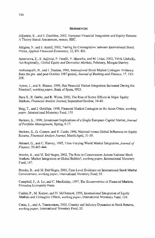
114

REFERENCES

Adjaoute, K., and 1 Danthine, 2002, European Financial Integration and Equity Returns:A Theory Based Assessment, mimeo, HEC.

Ahlgren, N. and 1 Antell, 2002, Testing for Cointegration between International StockPrices, Applied Financial Economics, 12, 851-861.

Ametisova, E., S. Anjilvel, P. Fanelli, Y. Sharaiha, and M. Urias, 2002, Think Globally,Act Regionally, Global Equity and Derivative Markets, February, Morgan Stanley.

Arshanapalli, B., and J. Doukas, 1993, International Stock Market Linkages: Evidencefrom the pre- and post October 1987 period, Journal ofBanking and Finance, 17, 193­208.

Ayuso, 1, and R. Blanco, 1999, Has Financial Market Integration Increased During theNineties?, working paper, Bank of Spain, 9923.

Baca S., B. Garbe, and R. Weiss, 2000, The Rise of Sector Effects in Major EquityMarkets, Financial Analyst Journal, September/October, 34-40.

Baig, T., and 1. Goldfajn, 1998, Financial Market Contagion in the Asian Crisis, workingpaper, International Monetary Fund, 155.

Beckers, S., 1999, Investment Implications of a Single European Capital Market, JournalofPortfolio Management, Spring, 9-17.

Beckers, S., G. Connor, and R. Curds, 1996, National versus Global Influences on EquityReturns, Financial Analyst Journal, March/April, 31-39.

Bekaert, G., and C. Harvey, 1995, Time-Varying World Market Integration, Journal ofFinance, 50,403-444.

Brooks, R., and M. Del Negro, 2002, The Rise in Comovement Across National StockMarkets: Market Integration or Global Bubble?, working paper, International MonetaryFund, 147.

Brooks, R., and M. Del Negro, 2003, Finn-Level Evidence on International Stock MarketComovement, working paper, International Monetary Fund, 55.

Campbell, J., A. Lo, and C. MacKinlay, 1997, The Econometrics of Financial Markets,Princeton University Press.

Cashin, P., M. Kunlar, and D. McDernl0tt, 1995, International Integration ofEquityMarkets and Contagion Effects, working paper, International Monetary Fund, 110.

Catao, L., and A. Timmerman, 2003, Country and Industry Dynamics in Stock Retunls,working paper, International Monetary Fund, 52.

115

Cavaglia, S., C. Brightman, and M. Aked, 2000, The Increasing Importance of IndustryFactors, Financial Analyst Journal, September/October, 41-54.

Chan, C., & P. Lai, 1993, Unit root and Cointegration Tests of World Stock Prices, inStansell, S., ed., International Financial Market Integration, Blackwell.

Chen, G., M. Firth, and 0 Rui, 2002, Stock Market Linkages: Evidence from LatinAmerica, Journal ofBanking and Finance, 26, 1113-1141.

Danthine, J., F. Giavazzi, E. von Thadden, 2000, European Financial Markets AfterEMU: A First Assessment, mimeo, UNU/WIDER project on EMU.

Davis, E. P., and D. Steil, 2001, Institutional Investors, MIT Press, London.

DeRyck K., 1998, Asset Allocation, Financial Market Behavior and Impact ofEUPension Funds on European Capital Markets, in OECDs Institutional Investors in theNew Financial Landscape, chapter 11.

Griffin, J., and A. Karolyi, 1998, Another Look at the Role of the Industrial Structure ofMarkets for International Diversification Strategies, Journal ofFinancial Economics, 50,351-373.

Fama, E., and 1. MacBeth, 1973, Risk, Return, and Equilibrium: Empirical Tests, JournalofPolitical Economy, 81, 607-636.

Fratzscher, M., 2001, Financial Market Integration in Europe: On the Effects of EMU onStock Markets, working paper, European Central Bank, 48.

Freimalill, E., 1998, Economic Integration and Country Allocation in Europe, FinancialAnalysts Journal, September/October, 32-41.

Forbes, K., and R. Rigobon, 2002, No Contagion, Only Interdependence: MeasuringStock Market Comovements, Journal ofFinance, 57, 2223-2261.

Hamilton, J., 1994, Time Series Analysis, Princeton University Press.

Heston, S., and G. Rouwenhorst, 1994, Does Industrial Structure Explain the Benefits ofInternational Diversification?, Journal ofFinancial Economics, 36, 3-27.

hltemational Monetary Fund, 2001, Emerging Market Financing: Developments andProspects, Febnlary, IMF.

Kose, M.A., E. Prasad, and M. Terrones, Financial Integration and MacroeconomicVolatility, mimeo, IMF Annual Research Conference, Washington.

Lannoo, K., 1998, Institutional Investors, Capital Markets and EMU, in DEeDsInstitutional Investors in the New Financial Landscape, chapter 15.

Ma C., 1993, Financial Market Integration and Cointegration Tests, in Stansell, S., ed.,International Financial Market Integration, Blackwell.

116

Masih A. & R. Masih, 1997, Dynamic Linkages and the Propagation Mechanism DrivingMajor International Stock Markets: An Analysis of the Pre- and Post-Crash Eras,Quarterly Review ofEconomics and Finance, 37, 859-885.

Niemeyer, J., 2001, An Economic Analysis of Securities Regulation and Supervision:Where to go after the Lamfalussy Report?, SSE/EFI working paper, 482.

Nystedt, J., 2000, De Svenska finansiella marlrnadernas integration med utlandet,Finansmarknadsutredningen, Bilaga 17.

Organization for Economic Co-operation and Development, 2001, Institutional InvestorsStatistical Yearbook 2001, OEeD.

Organization for Economic Co-operation and Development, 1998, Institutional Investorsin the New Financial Landscape, OECD.

Roll, R., 1992, Industrial Structure and the Comparative Behavior of International StockMarket Indices, Journal ofFinance, 47, 3-41.

Rouwenhorst, G., 1998, European Equity Markets and EMU: Are the Differences SlowlyDisappearing?, mimeo, Yale School ofManagement.

Solnik, B., C. Boucrelle and Y. Le Fur, 1996, International Market Correlation andVolatility, Financial Analysts Journal, September/October, 17-34.

Steil, B., ed., 1996, The European Equity Markets, RJIA.

Taylor, M., and 1. Tonks, 1989, The Internationalization of Stock Markets and theAbolition ofU.K. Exchange Controls, Review ofEconomic and Statistics, 332-336.

Tesar, L., and 1. Werner, 1995, Home Bias and High Turnover, Journal ofInternationalMoney and Finance, 14, 467-493.

Urias, M., Y. Sharaiha, and R. Hendricks, 1998, European Investing after EMU: hldustryand National Effects in Equity Returns, Global Equity and Derivative Markets, February,Morgan Stanley.

Warnock, F., 2002, Home Bias and High Turnover Reconsidered, Journal ofInternational Money and Finance, 21, 795-805.

117

EFIThe Economic Research Institute

Reports since 1999A complete publication list can be found at www.hhs.se/efi

Published in the language indicated by the title

2004Andersson, A., Essays in Behavioral Finance.Gronqvist, E., Selection and Moral Hazard in Health Insurance: Taking ContractTheory to the Data.Jutterstrom, M., Att paverka beslut - foretag i EUs regelsattande.Larsson, P., Forandringens villkor. En studie av organisatoriskt larande och fOrandringinom skolan.Lagerwall, B., Empirical Studies ofPortfolio Choice and Asset Prices.Malmsten, H., Properties and Evaluation ofVolatility Models.Nilsson, C., Studies in Environmental Economics: Numerical Analysis of GreenhouseGas Policies.Regelexplosionen. Ahme, G., Brunsson, N. (red).Salabasis, M., Bayesian Time Series and Panel Models - Unit Roots, Dynamics andRandom Effects.Skallsjo, S., Essays on Ternl Structure and Monetary Policy.Soderstrom, J., Fran Produkt till Tjanst. Utveckling av affars- och miljostrategier iproduktorienterade foretag.Talia, K., The Scandinavian Currency Union, 1873-1924 - Studies in MonetaryIntegration and Disintegration

2003Andersson, H., Valuation and Hedging of Long-Terrn Asset-Linked Contracts.Bergman, M., Essays on Human Capital and Wage Fonnation.Damsgaard, N., Deregulation and Regulation of Electricity Markets.Eklund, B., Four Contributions to Statistical Inference in Econometrics.Exploring Patterns in Information Management. Concepts and Perspectives forUnderstanding IT-Related Change. Sundgren, B, Mfuiensson, P., Mahring, M.,Nilsson, K., (editors)Globalization and its Enemies, Lundahl, M (editor).Hakkala, K., Essays on Restructuring and Production Decisions in Multi-Plant Finns.Holgersson, C., Rekrytering av foretagsledare. En studie i hoimosocialitet.Ivaschenko, I, Essays on Corporate Risk, U.S. Business Cycles, International Spilloversof Stock Returns, and Dual Listing.Lange, F., Brand Choice in Goal-derived Categories - What are the Detemlinants?Le Coq, C., Quantity Choices and Market Power in Electricity Market.Magnusson, P.R., Customer-Oriented Product Development - ExperimentsInvolving Users in Service Innovation.Meisiek, S., Beyond the Emotional Work Event Social Sharing ofEmotion inOrganizations.

118

Martensson, A.. Managing Mission-Critical IT in the Financial Industry.Nilsson, G., Processorientering och styrning - RegIer, mal eller varderingar?Sandberg, R., Corporate Consulting for Customer Solutions Bridging DivergingBusiness Logics.Sturluson, J.T., Topics in the Industrial Organization of Electricity Markets.Tillberg, U., Ledarskap och samarbete - En jarnforande fallstudie i tre skolor.Waldenstrom, D., Essays in Historical Finance.Wallen, D., Effektivitet i grundskolan i anslutning till en stadsdelsnfunndsrefonn.Ogren, A., Empirical Studies in Money, Credit and Banking - The Swedish CreditMarket in Transition under the Silver and the Gold Standards, 1834 - 1913.

2002Barinaga, E., Levelling Vagueness - A study of cultural diversity in an internationalproject group.Berglund, J., De otillrackliga - En studie av personalspecialisternas kamp forerkannande och status.Bolander, P., Anstallningsbilder och rekryteringsbeslut.Damjanovic, T., Essays in Public Finance.Ekman, M., Studies in Health Economics - Modelling and Data Analysis of Costs andSurvival.Foretagerskan - Om kvinnor och entreprenorskap. Holmquist, C. och Sundin, E (red)Heyman, F., Empirical Studies on Wages, Firm Perfonnance and Job Turnover.Kallifatides, M., Modem foretagsledning oeh omoderna foretagsledare.Kaplan, M., Acquisition ofElectronic Commerce Capability - The Cases of Compaq andDell in Sweden.Mahring, M., IT Project Governance.Nilsson, M., Essays in Enlpirical Corporate Finance and Governance.Rekrytering av koncernstyrelsen - Nomineringsforfaranden ochstyrelsesammansattning med focus pa kvinnors stallning och mojIigheter.Sjostrand, S-E. och Petrelius, P.,(red)Scener ur ett foretag - Organiseringsteori for kunskapssamhallet. Lowstedt, J.Stymne, B.,(red).Schenkel, A., Communities ofPractice or Communities ofDiscipline - ManagingDeviations at the 0resund Bridge.Schuster, W., Foretagets Valutarisk - En studie av horisontella och vertikalastyrprocesser.Skogsvik, S., Redovisningsmatt, varderelevans och informationseffektivitet.Sunden, D., The Dynamics ofPension Refonn.Ternstrom, I., The Management of Common-Pool Resources - Theoretical Essaysand Empirical Evidence.Tullberg, J., Reciprocitet - Etiska nonner och praktiskt samarbete.Westling, G., Balancing Innovation and Control- The Role ofFace-to-face Meetings inComplex Product Development Projects.Viklund, M., Risk Policy - Trust, Risk Perception, and Attitudes.Vlachos, J., Risk Matters - Studies in Finance, Trade and Politics.

2001Adolfson, M., Monetary Policy and Exchange Rates - Breakthrough ofPass-Through.

119

Andersson, P., Expertise in Credit Granting: Studies on Judgment and Decision-Makingbehavior.Bjorklund, C., Work Motivation - Studies of its Determinants and Outcomes.Center for Management and Organization 50 (1951-2001).Charpentier, C., Uppf61jning av kultur- och fritidsforvaltningen efter stadsdelsnamnds­refonnen.Dahlen, M., Marketing on the Web - Empirical Studies of Advertising and PromotionEffectiveness.Eckerlund, I., Essays on the Economics ofMedical Practice Variations.Ekelund, M., Competition and Innovation in the Swedish Pharmaceutical Market.Engstrom, S., Success Factors in Asset Management.Ericsson, D., Kreativitetsmysteriet - Ledtradar till arbetslivets kreativisering ochskrivandets metafysik.Eriksson, R., Price Responses to Changes in Costs and Demand.Frisell, L., Infonnation and Politics.Giordani, P., Essays in Monetary Economics and Applied Econometrics.Gustavsson, P., Essays on Trade, Growth and Applied Econometrics.Hedlund, A., Konsumentens erfarenhet - och dess inverkan pa livsmedelsinkop paInternet.Hill, M., Essays on Environmental Policy Analysis: Conlputable General EquilibriumApproaches Applied to Sweden.Hvenmark, J., Varfor slocknar elden? Om utbrandhet bland chefer i ideella organisa­tioner.Hagglund, P.B., Foretaget som investeringsobjekt - Hur placerare och analytiker arbetarmed att ta franl ett investeringsobjekt.Hook, P., Stridspiloter i vida kjolar, om ledarutveckling ochjamsHilldhet.Johansson, C., Styrning for samordning.Josephson, J., Evolution and Learning in Ganles.Kjellberg, H., Organising Distribution - Hakonbolaget and the efforts to rationalise fooddistribution, 1940-1960.Lange, F. och Wahlund, R., Category Management - Nar konsumenten ar manager.Liljenberg, A., Customer-geared competition - A socio-Austrian explanation of TertiusGaudens.Lindkvist, B., Kunskapsoverforing nlellan produktutvecklingsprojekt.Ljunggren, U., Nyckeltal i grundskolan i Stockholms stad fore och efter stadsdels­namndsrefornlen.Lakemedel- Kostnad eller resurs for sjukvarden? Jonsson, B.,(red).Lof, M., On Seasonality and Cointegration.Martensen, K., Essays on Entry Externalities and Market Segmentation.Matros, A., Stochastic Stability and Equilibrium Selection in Gan1es.Martensson, P., Management Processes - An Information Perspective on ManagerialWork.Nilsson, A., Market Transparency.Norberg, P., Finansmarknadens amoralitet och det kalvinska kyrkonnnmet - En studie iekonomisk mentalitet och etik.Persson, B., Essays on Altruism and Health Care Markets.Rech, G., Modelling and Forecasting Economic Time Series with Single Hidden-layerFeedforward Autoregressive Artificial Neural Networks.Skoglund, J., Essays on Random Effects Models and GARCH.Strand, N., En1pirical Studies ofPricing.

120

Thoren, B., Stadsdelsnamndsreformen och det ekonomiska styrsystenlet - Om budgetav­vikelser.

2000Berg-Suurwee, D., Styrning fore och efter stadsdelsnfunndsreform inonl kultur ochfritid - Resultat fran intervjuer och enkat.Bergkvist, L., Advertising Effectiveness Measurement: Intermediate Constructs andMeasures.Brodin, B., Lundkvist, L., Sjostrand, S-E., Ostman, L., Koneemchefen och agama.Bornefalk, A., Essays on Social Conflict and Reform.Charpentier, C., Samuelson, L.A., Effekter av en sjukvardsrefonn.Edman, J., Information Use and Decision Making in Groups.Emling, E., Svenskt fanriljeforetagande.Ericson, M., Strategi, kalkyl, kansla.Gunnarsson, J., Wahlund, R., Flink, H., Finansiella strategier i forandring: segmentoch beteenden bland svenska hushal1.Hellman, N., Investor Behaviour - An Empirical Study ofRow Large SwedishInstitutional Investors Make Equity Investment Decisions.Hyll, M., Essays on the Term Structure of Interest Rates.Hakansson, P., Beyond Private Label- The Strategic View on Distributor Own Brands.I huvudet pa knnden. Soderlund, M (red). EFI oeh Liber Forlag.Karlsson Stider, A., Familjen och firman.Ljunggren, D., Styrning av grundskolan i Stockholms stad fore och efter stadsdels­namndsreformen - Resultat fran intervjuer oeh enkat.Ludvigsen, J., The futemational Networking between European Logistical Operators.Nittmar, H., Produktutveckling i samarbete - Strukturfdrandring vid inforande av nyafuformationssystem.Robertsson, G., International Portfolio Choice and Trading Behavior.Schwarz, B., Weinberg, S., Serviceproduktion oeh kostnader - aU soka orsaker tillkommunala skillnader.Stenstrom, E., Konstiga fdretag.Styrning av team och processer - Teoretiska perspektiv och fallstndier. Bengtsson,L., Lind, J., Samuelson, L.A., (red).Sweet, S., Industlial Change Towards Environmental Sustainability - The Case ofReplacing Chloroflouorocarbons.Tamm Hallstrom, K, Kampen for auktoritet - standardiseringsorganisationer i arbete.

1999Adler, N., Managing Complex Product Development.Allgulin, M., Supervision and Monetary Incentives.Andersson, P., Experto Credite: Three Papers on Experienced Decision Makers.Ekman, G., Fran text till batong - Om poliser, busar och svennar.Eliasson, A-C., Smooth Transitions in Macroeconomic Relationships.Flink, H., Gunnarsson, J., Wahlund, R., Svenska hushallens sparande oeh skuld­sattning- ett konsumentbeteende-perspektiv.Gunnarsson, J., Portfolio-Based Segmentation and Consumer Behavior: EmpiricalEvidence and Methodological Issues.

121

Hamrefors, S., Spontaneous Environmental Scanning.Helgesson, C-F., Making a Natural Monopoly: The Configuration of a Techno-EconomicOrder in Swedish Telecommunications.Japanese Production Management in Sunrise or Sunset. Karlsson, C., (red).Jonsson, B., Jonsson, L., Kobelt, G., Modelling Disease Progression and the Effect ofTreatment in Secondary Progressive MS. Research Report.Linde, J., Essays on the Effects ofFiscal and Monetary Policy.Ljunggren, U., Indikatorer i grundskolan i Stockholms stad fore stadsdelsnamnds­reformen - en kartlaggning.Ljunggren, U., En utvardering av metoder for att mata produktivitet och effektivitet iskolan - Med tillampning i Stockholms stads grundskolor.Lundbergh, S., Modelling Economic High-Frequency Time Series.Magi, A., Store Loyalty? An Empirical Study of Grocery Shopping.Molleryd, B.G., Entrepreneurship in Technological Systems - the Development ofMobile Telephony in Sweden.Nilsson, K., Ledtider for ledningsinfonnation.Osynlig Foretagsledning. Sjostrand, S-E., Sandberg, J., Tyrstrup, M., (red).Rognes, J., Telecommuting - Organisational Impact ofRome Based - Telecommuting.Sandstrom, M., Evaluating the Benefits and Effectiveness ofPublic Policy.Skalin, J., Modelling Macroeconomic Time Series with Smooth TransitionAutoregressions.Spagnolo, G., Essays on Managerial Incentives and Product-Market Competition.Strauss, T., Governance and Structural Adjustment Programs: Effects on Investn1ent,Growth and Income Distribution.Svedberg Nilsson, K., Effektiva foretag? En studie av hur privatiserade organisationerkonstrueras.Soderstrom, U., Monetary Policy under Uncertainty.Werr, A., The Language of Change The Roles of Methods in the Work of ManagementConsultants.Wijkstrom, F., Svenskt organisationsliv - Framvaxten av en ideell sektor.