Competition, Product Proliferation and Welfare: A Study of the

U.S. Smartphone Market∗

Ying Fan†

University of Michigan, CEPR and NBER

Chenyu Yang‡

University of Rochester

June 4, 2018

Click Here for the Latest Version

Abstract

This paper studies (1) whether, from a welfare point of view, oligopolistic competition leads

to too few or too many products in a market, and (2) how a change in competition affects the

number and the composition of product offerings. We address these two questions in the context

of the U.S. smartphone market. Our findings show that this market contains too few products

and that a reduction in competition decreases both the number and variety of products. These

results suggest that product choice adjustment may exacerbate the welfare effect of a merger.

Key words: endogenous product choice, product proliferation, merger, smartphone industry

JEL Classifications: L13, L15, L41, L63

1 Introduction

In many markets such as the printer market, the CPU market and the smartphone market,

firms typically offer multiple products across a wide spectrum of quality. In these markets, product

proliferation is an outcome of firms’ oligopolistic competition in product space. Does such compe-

tition result in too few or too many products from a welfare point of view? How does a change in

the level of competition affect the number and composition of product offerings? In this paper, we

study these two questions in the context of the U.S. smartphone industry.

∗We thank participants at the 2016 Barcelona GSE Summer Forum, the 2016 CEPR/JIE Applied IO conference,the 2016 Econometric Society North American Summer Meeting, the 2017 Econometric Society Asian and Chinameeting, the 2017 HEC Montreal-CIRANO-RIIB Conference on Industrial Organization, the 2015 InternationalIndustrial Organization Conference, the 2016 NBER Summer Institute IO Workshop, and the 2015 World Congressof the Econometric Society, and participants at many seminars for their constructive comments. We thank theMichigan Institute for Teaching and Research in Economics, the NET Institute and Rackham Graduate School ofthe University of Michigan for their generous financial support.†Department of Economics, University of Michigan, 611 Tappan Street, Ann Arbor, MI 48109; yingfan@umich.edu.‡Simon Business School, University of Rochester, Rochester, NY 14627; chny.yang@gmail.com.

1

For the first question, in theory, it is possible that oligopolistic competition results in either too

few or too many products. On the one hand, because firms do not take into account the business

stealing externality, there may be too many products. On the other hand, because firms do not

internalize consumer surplus, there may also be too few products. These two effects, which work

in opposite directions, are highlighted in Spence (1976) and Mankiw and Whinston (1986) in the

context of a single-product oligopoly. In a multi-product oligopoly, however, there exists another

factor influencing the equilibrium product offerings: firms’ incentives to avoid cannibalization of

their own products, which may drive the equilibrium towards too few products. Overall, because

of these factors, whether competition leads to too few or too many products in the market is an

empirical question.

For the second question, the effect of a merger on product offerings is also theoretically ambigu-

ous. When two firms merge, the merged firm internalizes the business stealing effect and thus may

reduce its number of products. This is a direct effect. However, there may also exist a countervail-

ing indirect effect: a merger is likely to soften price competition. As a result, the profit gains from

adding a product may be larger, leading to an increase in the number of products.

Combining these two research questions, this paper sheds light on how to adjust the leniency

of competition policies when product offerings are endogenous. If competition leads to too many

products and a merger reduces product offerings, then merger policies may need to be more lenient.

Conversely, if a merger reduces product offerings when there are already too few products in the

market, then merger policies may need to be stricter.

Product variety is an important determinant of welfare, and firms’ product portfolio may be an

important margin of adjustment after a merger. Section 6.4 of the 2010 Horizontal Merger Guide-

lines, for example, states that antitrust agencies consider the welfare effects of mergers through the

adjustment of product variety: “Mergers can lead to the efficient consolidation of products . . . In

other cases, a merger may increase variety . . . If the merged firm would withdraw a product that a

significant number of customers strongly prefer to those products that would remain available, this

can constitute a harm to customers over and above any effects on the price or quality of any given

product. If there is evidence of such an effect, the Agencies may inquire whether the reduction in

variety is largely due to a loss of competitive incentives attributable to the merger.”

We study our research questions in the context of the U.S. smartphone market. The smartphone

industry has been one of the fastest growing industries in the world, with billions of dollars at stake.

Worldwide smartphone sales grew from 122 million units in 2007 to 1.4 billion units in 2015 (Gartner

(2007) and Gartner (2015)), with about 400 billion dollars in global revenue in 2015 (GfK (2016)).

Moreover, product proliferation is a prominent feature of this industry. For example, in the U.S.

market during our sample period, Samsung, on average, simultaneously offered 11 smartphones

with substantial quality and price variation.

In order to address our research questions, we develop a structural model of consumer demand

and firms’ product and pricing decisions, and estimate the model using data from the Investment

2

Technology Group (ITG) Market Research. This data set provides information on all smartphone

products in the U.S. market between January 2009 and March 2013. For every month during this

period, we observe both the price and the quantity of each smartphone sold through each of the

four national carriers in the U.S. (AT&T, T-Mobile, Sprint, and Verizon). In addition, we observe

key specifications of each product, such as battery talk time and camera resolution.

Using these data, we estimate our model of smartphone demand and supply. The estimation

results are intuitive: on average and ceteris paribus, consumers prefer smartphones with longer

battery talk time, higher camera resolution, a more advanced chipset, a larger screen, and a lighter

weight. We use these results to calculate a product quality index, a linear combination of product

characteristics weighted by the corresponding estimated demand coefficients. We then use our

quality index to propose a measure of product variety such that adding a product identical to

an existing product in terms of the observed key characteristics has no impact on our variety

measure. Therefore, this measure allows us to distinguish “meaningful” product differentiation from

obfuscation. Our results show that product variety within the U.S. smartphone market increases

over time during our sample.

On the supply side, we find that marginal cost increases in quality. We also obtain bounds on

fixed costs. Specifically, we assume that the observed product portfolio of a smartphone firm is

profit maximizing in a Nash equilibrium. Consequently, removing or adding a product should not

increase the firm’s profit. Based on these conditions, for any product in the market in a month, we

obtain an upper bound of its fixed cost in that month; and for any product not in the data in a

given month, we obtain a lower bound.

Based on the estimated demand, marginal cost and fixed cost bounds, we conduct counterfactual

simulations to address our research questions. To answer the question of whether there are too few

or too many products in the market, we conduct two sets of counterfactual simulations for March

2013, the last month in our sample period. In one set of counterfactual simulations, we remove

products while in the other set, we add products. Our results show that removing a product

decreases total surplus, even considering the maximum saving in the fixed cost. These results are

robust no matter which product or which two products we remove. In the second set of simulations,

we add a product that fills a gap in the quality spectrum. We find that consumer surplus, carrier

surplus, and smartphone firms’ total variable profit all increase. The change in total welfare is

the sum of these increases minus the fixed cost of the added product. We find that the former

is about 2.3 times the lower bound of the latter. Therefore, as long as the fixed cost is not more

than 2.3 times its lower bound, total surplus increases. To put this ratio in perspective, note that

the average of all estimated upper bounds is about 1.2 times the average lower bound. Overall,

these counterfactual simulation results suggest that there are too few products under oligopolistic

competition.

Turning to the second research question of how a change in competition affects product offerings,

we simulate the effect of a hypothetical merger between Samsung and LG in March 2013. We also

3

repeat the simulation for a Samsung-Motorola merger and an LG-Motorola merger. Different

from addressing the first research question, for which we only need to compute the new pricing

equilibrium given certain product offerings in the market, we now need to compute the post-

merger equilibrium in both product choice and pricing. Computing the product-choice equilibrium

is challenging because, in theory, a firm can drop any subset of its current products or add any

number of new products after a merger, leading to a large action space. To keep the problem

tractable, we restrict the set of potential products for each firm to those offered by this firm in

either February or March 2013, plus two additional products that vary in quality. Even with this

restriction, a firm’s action space can still be prohibitively large. For example, the merged Samsung-

LG entity has 36 potential products, implying a choice set of 236 (≈ 6.9× 1010) product portfolios.

Therefore, to further deal with this computational challenge, we use a heuristic algorithm to find

a firm’s best-response product portfolio given the portfolios of its competitors, and embed this

optimization algorithm in a best-response iteration to solve for the post-merger product-choice

equilibrium. Results from Monte Carlo simulations show that our algorithm performs well at least

for optimal product portfolio problems with a small number of potential products.1

Using this algorithm, we find that after the Samsung-LG merger, the number of products in

the market decreases. On average, the merged firm drops three products while competing firms

altogether add one product. This reduction in the overall number of products also decreases product

variety. Due to the decrease in product offerings and the accompanying increase in the prices, we

find that consumers are worse off and total welfare also decreases after the merger. These findings

hold for the other two mergers as well (Samsung-Motorola and LG-Motorola).

In summary, we find that there are too few products in the market. We also find that a reduction

in competition as a result of a merger further decreases product variety. These findings are robust

to an extensive list of variations to the demand side of the model (4 such robustness analyses), to

the supply side (5 such robustness analyses) and to the merger simulation specifications (7 such

robustness analyses).

By studying the welfare implications of product proliferation and how competition affects them,

this paper contributes to the literature of endogenous product choice. Examples in this literature

include Draganska, Mazzeo and Seim (2009), Fan (2013), Sweeting (2013), Eizenberg (2014), Nosko

(2014), Berry, Eizenberg and Waldfogel (2016) and Wollmann (2018).2 In terms of methodology,

the paper is closely related to Eizenberg (2014), which also studies multi-product firms’ discrete

product choice for a different research question. Thus, both papers face the challenge of computing

1In the Monte Carlo simulations, we study product-choice problems where the number of potential products issmall enough for us to enumerate all possible product portfolios and determine the optimal one. We find that thefailure rate for the heuristic algorithm (i.e., the percentage of simulations where the heuristic algorithm fails to findthe true optimal product portfolio) is always lower than 0.6% even as we increase the number of potential productsto 10.

2Other examples include Seim (2006), Watson (2009), Chu (2010), Crawford and Yurukoglu (2012), Crawford,Shcherbakov and Shum (2015), Orhun, Venkataraman and Chintagunta (2015) and Hristakeva (2016). See Crawford(2012) for a survey of this literature. Examples in the theoretical literature on this topic include Johnson and Myatt(2003) and Shen, Yang and Ye (2016).

4

an equilibrium where firms have a large discrete choice set in the counterfactual simulations. We

tackle the problem using different approaches though. Eizenberg (2014) directly restricts the firms’

choice set to the extent that there are only 512 possible equilibrium configurations. This approach

is reasonable in his setting because Eizenberg (2014) studies the effect of removing a product. It is

therefore plausible to assume that products that are not close substitutes do not adjust. Our paper

focuses on mergers. It is unclear, ex ante, which products are unlikely to be adjusted. We thus

take a different approach as explained before. In terms of topics, this paper is closely related to

Fan (2013), which also studies the effect of a merger considering firms’ endogenous product choices.

However, whereas Fan (2013) keeps the number of products fixed, our model allows firms to adjust

both the number and composition of products after a merger. Interestingly, despite the differences

in focus and industries, the two papers make similar policy recommendations: merger policies may

need to be tougher when we take into account firms’ post-merger adjustments in their product

portfolios, whether such adjustments only concern the characteristics of a fixed set of products or

also involve changes in the number of products. By contrast, Wollmann (2018) finds that product

adjustments mitigate the negative merger effect in the commercial truck industry, while we find

that they exacerbate it in the smartphone industry. Note that both papers find product exits by

the merging parties and product entries by non-merging firms. The difference is about the net

change in product offerings. One potential explanation for the difference is that the commercial

truck industry is segmented by gross vehicle weight rating.3 In such a market, the merged firm

would hold near monopoly power in some segments and earn high markups if there were no product

adjustments. Other firms thus have strong incentives to enter these segments, which alleviates the

harm of the merger. The smartphone market, on the other hand, is much less segmented. Here,

a merger does not dramatically increase concentration (and thus does not generate strong entry

incentives) in any “segment”. As a result, the incentive to avoid cannibalization dominates, and the

merged firm drops more products than what other firms add. Therefore, due to these differences

in market structure, Wollmann (2018) is more about the potential entry defense used in antitrust

and this paper is more about an antitrust authority’s concern regarding the (potentially negative)

merger effect on product variety.

This paper is also related to the stream of research that studies the smartphone industry. For

example, Sinkinson (2014) studies the motivations behind the exclusive contract between Apple

and AT&T for the early iPhones. In another study, Zhu, Liu and Chintagunta (2015) quantify the

welfare effects of this exclusive contract. Luo (2016) examines the operation system network effect.

Yang (2017) studies the effect of vertical integration on innovation in the smartphone industry and

its upstream chipset industry. Finally, Wang (2018) studies how a Chinese policy that induced

fringe entry affects incumbent firms’ product portfolio choices in the Chinese smartphone market.

3According to Wollmann (2018), “GWR [gross vehicle weight rating] determines the possible uses of a vehicle.Since carrying loads in excess of it is illegal and unsafe, and since it increases price, buyers purchase vehicles withthe minimum GWR that safely covers their needs.”

5

We complement these papers by studying the welfare implications of product choices and the effects

of competition with endogenous product choice.

The rest of the paper is organized as follows. We describe the data in Section 2. We develop

the model of the smartphone market in Section 3 and present the estimation results in Section 4.

Section 5 first describes counterfactual simulations and then discusses the results. We discuss the

robustness of the results in Section 6. Finally, we conclude in Section 7.

2 Data

Our data come from the Investment Technology Group (ITG) Market Research. This data set

covers all smartphones sold in the U.S. market between January 2009 and March 2013. For every

carrier in the U.S. and every month during our sample period, we observe the price and sales for

each smartphone sold through that carrier in that month. We also observe key specifications of

each product such as battery talk time and camera resolution.

The price information provided by the ITG for the four major national carriers (AT&T, Verizon,

Sprint, and T-Mobile) is the so-called subsidized price or the average price for a smartphone device

that a carrier charges a consumer who uses this carrier’s network service.4 Note that the subsidized

price for a smartphone is not the true cost of buying the smartphone because the consumer also

needs to pay for the service plan. As will be explained later, we include carrier/year-specific fixed

effects in the model to capture the average service cost for a consumer.

Furthermore, since non-major or fringe carriers serve only one regional market and often provide

only prepaid service plans, we drop these observations from our analyses.5 In the end, our sample

consists of 3256 observations, each of which is a smartphone/carrier/month combination. Table 1

presents the summary statistics on the quantity, price and product characteristics. The average

monthly sales of a product are around 77,000 while the standard deviation of the monthly sales

is about twice the mean. There is also a sizable variation in price across observations: the price

is 122 dollars on average, with a standard deviation of 85. For each product, we observe product

characteristics such as battery talk time, camera resolution, screen size measured by the diagonal

length of the screen, and weight. We also observe the generation of the chipset used by each

product. For example, there are five Apple smartphones in our data (i.e., iPhone 3G, iPhone 3Gs,

iPhone 4, iPhone 4s and iPhone 5), each of which uses a chipset of a different generation. The

standard deviations of these product characteristics are about 17% to 47% of their corresponding

means, indicating a wide variety of products across our sample.

There are 18 smartphone firms and 260 smartphones in the sample. Table 2 lists the top six

firms according to their average monthly smartphone sales: Apple, Samsung, BlackBerry, HTC,

4The average is taken over transactions in a month. Note that the carrier fee structure is relatively stable during oursample period. In April 2013 (right after our sample period), however, T-Mobile launched an “Uncarrier” campaign,which abandoned service contracts and subsidies for devices. Other carriers followed suit.

5The total U.S. market share of these fringe carriers in terms of smartphones sold is about 10%.

6

Table 1: Summary Statistics

Variable Mean Std. Dev. Min Max

Quantity (1000) 77.54 146.04 0.04 1419Price ($) 122.16 85.24 0a 406.9Battery talk time (hour) 7.08 2.93 3 22Camera resolution (megapixel) 4.65 2.18 0b 13Chipset generation 2 dummy 0.23 0.42 0 1Chipset generation 3 dummy 0.25 0.43 0 1Chipset generation 4 dummy 0.14 0.34 0 1Chipset generation 5 dummy 0.09 0.29 0 1Screen size (inch) 3.44 0.73 2.20 5.54Weight (gram) 135.31 22.72 89.5 193

Observations (smartphone/carrier/months) 3256aFour observations in our sample have a 0 price.bOne product in our sample (BlackBerry 8830) does not have a camera.

Motorola and LG. From Table 2, we see that Apple is the leader in the industry, with an average

monthly sales of about 2 million units, followed by Samsung with an average monthly sales of 0.76

million units. The table also shows that all of these six firms offer multiple products simultaneously.

For example, on average, Samsung offers 11 products in a given month, followed by HTC with an

average of 10 products in a given month.

Table 2: List of Top Six Smartphone Firms

Firm Headquarters Avg. Monthly Salesa Avg. Number(million units) of Productsa

Apple U.S. 1.99 2.10Samsung Korea 0.76 11.08BlackBerry Canada 0.61 8.33HTC Taiwan 0.60 10.35Motorola U.S. 0.46 7.90LG Korea 0.33 6.76aAveraged across months.

To see whether the multiple products offered by a smartphone firm are similar or different in

quality and price, in Table 3, we report two within-(firm/month) dispersion measures for price and

product characteristics. To calculate within-(firm/month) price dispersion, for example, we first

compute the standard deviation of price across all observations of a given firm/month combination.

We set the standard deviation to 0 for firm/months with a single observation. We then take the

average of these standard deviations across all 557 firm/months in the sample, and report this

average in Column 1 of Table 3. Similarly, we compute the difference between the highest and the

lowest price among all observations in the same firm/month and take the average across firm/months

to obtain the average range within a firm/month, as shown in Column 2. We find that the average

7

within-(firm/month) standard deviation in price is 42.42 dollars, which is about 1/2 of the overall

standard deviation of price across all observations (see Table 1), implying that within-(firm/month)

variation is an important component of total price variation. The within-(firm/month) variation

of product characteristics is also significant. For example, Column 2 for chipset generation shows

that smartphone firms on average simultaneously offer products whose chipsets are one generation

apart. Overall, Table 3 provides evidence for product proliferation in the smartphone industry.

Table 3: Summary Statistics on Quality and Price Dispersion within a Firm/Month

Average Std. Dev. Average Range

Price ($) 42.42 122.50Battery talk time (hour) 1.04 3.10Camera resolution (megapixel) 0.81 2.16Chipset generation 0.36 0.93Screen size (inch) 0.21 0.61Weight (gram) 11.12 32.23

3 Model

3.1 Demand

We use a random-coefficient discrete choice model to describe smartphone demand. Since our

data are aggregated to the smartphone/carrier/month level, we assume that a consumer’s choice

is a smartphone/carrier combination, indexed by j. Furthermore, we assume that the utility that

consumer i gets from purchasing j in period t is:

uijt = βiqj − αpjt + λm(j) + κc(j)t + ξjt + εijt, (1)

where qj is a quality index which depends on the observable product characteristics xj as qj =

xjθ, where θ are parameters to be estimated.6 The random coefficient βi captures consumers’

heterogeneous tastes for quality and is assumed to follow a normal distribution with mean β and

variance σ2. Since we cannot separately identify β, σ and θ as they enter the utility function as

βθ and σθ, we normalize the first element of θ to be 1. Finally, we denote the price of j in period

t by pjt.

To capture consumers’ average taste for a brand, we include a brand fixed effect, λm(j), where

m (j) represents the smartphone firm (i.e., the brand) of j. To capture the average quality and

6In other words, we assume that the consumer utility depends on the product characteristics only through thequality index. This parsimonious functional form allows us to estimate the heterogeneous preferences for all importantphone characteristics even if some of the characteristics’ own random coefficient variances cannot be estimatedprecisely, due to lack of variation, if we allow each characteristic to have an independent random coefficient. InAppendix B, we conduct a robustness analysis where we use the baseline estimates but assume that the coefficientsare independent across characteristics. We find our results are robust.

8

fees of carrier c’s network service in period t as well as a general time trend in consumers’ tastes

for smartphones, we include a carrier/year fixed effect.7 Finally, to capture seasonality in demand,

we include a quarter fixed effect. For simplicity of notation, we denote both the carrier/year fixed

effect and the quarter fixed effect by one term κc(j)t, where c (j) represents the carrier of choice j.

The term ξjt represents a demand shock, and the error term εijt captures consumer i’s idiosyncratic

taste, which is assumed to be i.i.d. and to follow a type-I extreme value distribution. We normalize

the mean utility of the outside option to be 0. Thus, the utility of the outside option is ui0t = εi0t.

Under the type-I extreme value distributional assumption of εijt, we can express the market

share of choice j in period t as:

sjt (qt,pt, ξt) =

∫exp

(βiqj − αpjt + λm(j) + κc(j)t + ξjt

)1 +

∑j′∈Jt exp

(βiqj′ − αpj′t + λm(j′) + κc(j′)t + ξj′t

)dF (βi) , (2)

where Jt denotes the set of all choices in period t, qt = (qj , j ∈ Jt), and pt and ξt are analogously

defined. Finally, F (βi) represents the distribution function of the random coefficient βi.

We define the mean utility of j in period t as

δjt = βqj − αpjt + λm(j) + κc(j)t + ξjt, (3)

and invert it out based on equation (2) following Berry, Levinsohn and Pakes (1995).

3.2 Supply

We use a static three-stage game to describe the supply side of the model. In the first stage,

smartphone firms choose their products. In the second stage, they choose the wholesale prices

charged to the carriers based on realized demand and marginal cost shocks. In the third stage,

carriers choose the subsidized retail prices. We describe these three stages in reverse order.

3.2.1 Decision on Prices

In the final stage of our model, carriers choose retail prices after observing the set of products

available on each carrier (denoted by Jct), wholesale prices (wjt) and demand shocks (ξjt). Suppose

that the profit that carrier c obtains through its service is bct per consumer. Thus, carrier c’s profit

for each unit of a product sold is pjt+bct−wjt. We do not observe bct or wjt. However, we can invert

out w̃jt = wjt−bc(j)t from the first-order condition on pjt. Specifically, carrier c’s profit-maximizing

7By using fixed effects to capture service plan features and prices, we implicitly assume that they are exogenous.We do so for two reasons. First, we do not have data on carriers’ service plans. It is also difficult to compare serviceplans provided by different carriers as they differ in many dimensions. Second, a carrier typically does not redesignits service plans when a new smartphone is introduced to the market. Thus, it is plausible to assume that carriers’service plans are exogenous to smartphone firms’ product and price decisions.

9

problem is

maxpjt,j∈Jct

∑j∈Jct

Nsjt (qt,pt, ξt) (pjt − w̃jt) , (4)

where N is the market size. The first-order condition allows us to invert out w̃jt as:

w̃jt = pjt + [∆−1ct sct]jt, (5)

where ∆ct represents a |Jct| × |Jct| matrix whose (j, j′) element is∂sj′t∂pjt

, and sct = (sjt, j ∈ Jct).We denote the equilibrium of this stage by p∗jt (w̃t, qt, ξt), where w̃t = (w̃jt, j ∈ Jt) and (qt, ξt)

are analogously defined in Section 3.1.

In the second stage, smartphone firms choose wholesale prices that they charge carriers after

observing demand and marginal cost shocks. We assume that marginal cost depends on product

quality (qj), carrier/year fixed effects (γct), and a jt-specific shock (ηjt).8 Specifically, we assume

that the marginal cost is mcjt = γc(j)t + γ1exp (qj) + ηjt.9 If we let m̃cjt = mcjt − bc(j)t and

γ̃c(j)t = γc(j)t − bc(j)t, we have:

m̃cjt = γ̃c(j)t + γ1 exp (qj) + ηjt. (6)

Note that w̃jt − m̃cjt = wjt − mcjt. A smartphone firm m’s profit-maximizing problem is

therefore

maxw̃jt,j∈Jmt

∑j∈Jmt

(w̃jt − m̃cjt)Nsjt (qt,p∗t (w̃t, qt, ξt) , ξt) , (7)

where Jmt represents the choices offered by firm m in period t. The first-order condition is

sjt +∑

j′∈Jmt

(w̃j′t − m̃cj′t

) ∑j′′∈Jt

∂sj′t∂pj′′t

∂p∗j′′t∂w̃jt

= 0, (8)

or equivalently,

w̃jt +[∆−1mtsmt

]jt

= γ̃c(j)t + γ1 exp (qj) + ηjt, (9)

where smt = (sjt, j ∈ Jmt), and ∆mt represents a |Jmt| × |Jmt| matrix whose (j, j′) element is(∑j′′∈Jt

∂sj′t∂pj′′t

∂p∗j′′t

∂w̃jt

). Combining equations (5) and (9) yields

pjt + [∆−1ct sct]jt +

[∆−1mtsmt

]jt

= γ̃c(j)t + γ1 exp (qj) + ηjt, (10)

which we bring to data for estimation.

8We allow marginal cost to vary across carriers because different radio technologies are used for products sold bydifferent carriers. Moreover, carriers sometimes require smartphone firms to preload specific software on a smartphone,contributing to cost differences.

9Following the literature, we assume that marginal cost is convex in quality (we expect γ1 to be positive) so thatthe profit function is concave in quality.

10

As can be seen from equation (10), this pricing model is a simple linear pricing model, which

implies double marginalization. In Section 6, we consider several alternative pricing models such

as a non-linear pricing model or a joint price setting model for robustness analyses.

3.2.2 Decision on Products

In the first-stage of the model, smartphone firms choose products. In other words, we assume

that the upstream firm makes the product decision, in contrast to Eizenberg (2014). Note that

in the PC market studied in Eizenberg (2014), the upstream firms (i.e., the CPU manufacturers)

produce only a component of the final product. Therefore, it seems natural to assume that the

downstream firms make a product decision in the PC market. In our setting, however, the upstream

firms make the final products directly, and it seems more natural to assume that they make the

product decisions. Nash equilibrium implies that given competitors’ product portfolios at the

equilibrium, any deviation from a smartphone firm’s equilibrium product portfolio should not lead

to a higher expected profit for this firm, where the expectation is taken over demand and marginal

cost shocks. Specifically, we consider two types of deviations: removing a product in the data or

adding a product not in the data. Note that while the majority of the products in our study are

sold through only one carrier, 12% are sold through multiple carriers. Therefore, to distinguish a

smartphone/carrier combination (indexed by j) from a smartphone product, we index the latter

by j̃. Similarly, J̃mt represents all smartphones of m, i.e., m’s product portfolio; and J̃t represents

all smartphones in the market in period t.

We first consider the case when a product is removed. Here, smartphone firm m’s expected

profit should not increase if product j̃ in its portfolio is removed, i.e.,

E(ξt,ηt)πmt (qt, ξt,ηt)− Fj̃t ≥ E(ξt\ξj̃t,ηt\ηj̃t)

πmt

(qt\qj̃ , ξt\ξj̃t,ηt\ηj̃t

)for any j̃ ∈ J̃mt, (11)

where πmt (qt, ξt,ηt) is the equilibrium variable profit for firm m (at the stage-2 and stage-3 pricing

equilibrium), Fj̃t is the fixed cost, πmt

(qt\qj̃ , ξt\ξj̃t,ηt\ηj̃t

)is firm m’s variable profit if product

j̃ is removed from its product portfolio, and Fj̃t is the fixed cost.10 Inequality (11) gives an upper

bound of Fj̃t for j̃t in the data. Intuitively, for products in the market, their fixed costs should be

bounded from above.

We next consider the case when a product is added. Here, firm m’s expected profit should

not increase if a potential product j̃ such that j̃ 6∈ J̃mt is added to its product portfolio. The

10If product j̃ is sold through multiple carriers, the fixed cost reflects the cost of having the product on the observedmultiple carriers. Therefore, later in counterfactual simulations, if a smartphone firm drops a product, it drops theproduct from all carriers. We have conducted robustness analyses where we re-estimate the fixed cost bounds foreach smartphone/carrier combination and allow firms to drop each smartphone/carrier separately. Our findings arerobust.

11

corresponding inequality is

E(ξt,ηt)πmt (qt, ξt,ηt) ≥ E(ξt∪ξj̃t,ηt∪ηj̃t)

πmt

(qt ∪ qj̃ , ξ ∪ ξj̃t,ηt ∪ ηj̃t

)− Fj̃t for any j̃ 6∈ J̃mt. (12)

This inequality yields a lower bound of Fj̃t for any j̃t such that j̃ 6∈ J̃t. This is again intuitive

because the fixed cost of a not-offered product should be bounded from below. Note that such

a potential product j̃ can be any product not in the data. In Sections 4 and 5, we explain the

potential products we consider in the estimation and the counterfactual simulations.

4 Estimation

4.1 Estimation Procedure

The estimation of demand and marginal costs is similar to that in Berry, Levinsohn and Pakes

(1995). We construct moments using equations (3) and (10), and estimate the parameters using the

Generalized Method of Moments. Following the literature, our instrumental variables are based on

the characteristics of other products of the same firm or the products of the competing firms. This

estimation strategy relies on the timing assumption that the demand and marginal cost shocks are

realized after the product choice.11 Note that we control for systematic brand effects, carrier effects,

and time effects using various fixed effects. Therefore, it seems reasonable (though imperfect) to

assume that any product/month-specific shocks are uncorrelated with product characteristics.12 In

addition to the above instruments, we include the four-month lagged exchange rates of the Chinese,

Japanese and Korean currencies to U.S. dollars as a cost shifter in the instruments. The market size

used in the estimation is 30 million, about 10% of the U.S. population during the sample period.

Our results are robust to other market size measures.

As for the fixed cost, we use inequalities (11) and (12) to obtain the bounds. Using inequal-

ity (11), we calculate the upper bound of Fj̃t as (the opposite of) the change in the expected variable

profit when product j̃ is removed, i.e., E(ξt,ηt)πmt (qt, ξt,ηt)−E(ξt\ξj̃t,ηt\ηj̃t)

πmt

(qt\qj̃ , ξt\ξj̃t,ηt\ηj̃t

).

The expectation is taken over the demand and marginal cost shocks (ξt,ηt). We assume that the

demand and marginal cost shocks each follow a normal distribution and obtain the estimates of

their means and standard deviations based on the estimated (ξ̂t, η̂t). To compute the expected

variable profit, we draw these shocks from their respective estimated distributions.13 We first com-

pute the pricing equilibrium and calculate the resulting variable profit for each draw, and then take

the average of these variable profits across all draws. Using inequality (12), we calculate the lower

11Similar timing assumption is made in, for example, Eizenberg (2014) and Wollmann (2018).12In Supplemental Appendix SA, we plot the estimated demand shocks ξ̂jt for three groups of observations sepa-

rately: (1) jt s.t. j is newly added to the market in period t; (2) jt s.t. j is discontinued after period t; and (3) allother jt. We find that the distributions of demand shocks do not seem to be very different across these three groups.This is also true for marginal cost shocks. While not a proof, these plots are assuring because the distributions couldbe quite different even under our exogeneity assumption.

13Our results are robust when we draw these shocks from their empirical distribution instead.

12

bound similarly for any j̃t such that j̃ 6∈ J̃t. Similar to Berry, Eizenberg and Waldfogel (2016), we

use these product/time-specific bounds directly in our welfare analyses instead of (set) estimating

a parametric function of the fixed cost. We do so to avoid making assumptions about the paramet-

ric functional form of the fixed cost and about its error terms (e.g., whether the error terms are

structural errors or measurement errors, and an independence assumption about the error terms).

However, there is a disadvantage of this approach: we implicitly assume that the total fixed cost

of a firm is the sum of the fixed cost for each product, which means we do not allow economies or

diseconomies of scope in fixed costs. To address this concern, we conduct a robustness analysis in

Appendix C where we assume a parametric function of the fixed cost and estimate the degree of

economies or diseconomies of scope in fixed costs following the moment inequality literature.14

4.2 Estimation Results

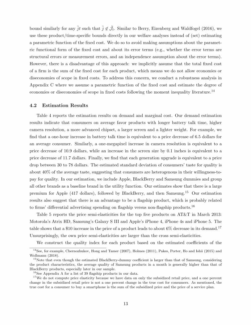
Table 4 reports the estimation results on demand and marginal cost. Our demand estimation

results indicate that consumers on average favor products with longer battery talk time, higher

camera resolution, a more advanced chipset, a larger screen and a lighter weight. For example, we

find that a one-hour increase in battery talk time is equivalent to a price decrease of 6.5 dollars for

an average consumer. Similarly, a one-megapixel increase in camera resolution is equivalent to a

price decrease of 10.9 dollars, while an increase in the screen size by 0.1 inches is equivalent to a

price decrease of 11.7 dollars. Finally, we find that each generation upgrade is equivalent to a price

drop between 30 to 78 dollars. The estimated standard deviation of consumers’ taste for quality is

about 40% of the average taste, suggesting that consumers are heterogenous in their willingness-to-

pay for quality. In our estimation, we include Apple, BlackBerry and Samsung dummies and group

all other brands as a baseline brand in the utility function. Our estimates show that there is a large

premium for Apple (417 dollars), followed by BlackBerry, and then Samsung.15 Our estimation

results also suggest that there is an advantage to be a flagship product, which is probably related

to firms’ differential advertising spending on flagship versus non-flagship products.16

Table 5 reports the price semi-elasticities for the top five products on AT&T in March 2013:

Motorola’s Atrix HD, Samsung’s Galaxy S III and Apple’s iPhone 4, iPhone 4s and iPhone 5. The

table shows that a $10 increase in the price of a product leads to about 6% decrease in its demand.17

Unsurprisingly, the own price semi-elasticities are larger than the cross semi-elasticities.

We construct the quality index for each product based on the estimated coefficients of the

14See, for example, Chernozhukov, Hong and Tamer (2007), Holmes (2011), Pakes, Porter, Ho and Ishii (2015) andWollmann (2018).

15Note that even though the estimated BlackBerry-dummy coefficient is larger than that of Samsung, consideringthe product characteristics, the average quality of Samsung products in a month is generally higher than that ofBlackBerry products, especially later in our sample.

16See Appendix A for a list of 39 flagship products in our data.17We do not compute price elasticity because we have data on only the subsidized retail price, and a one percent

change in the subsidized retail price is not a one percent change in the true cost for consumers. As mentioned, thetrue cost for a consumer to buy a smartphone is the sum of the subsidized price and the price of a service plan.

13

Table 4: Estimation Results

Parameter Std. Error

Demand

Quality coefficientbattery talk time (hour) 0.056∗∗∗ 0.013camera resolution (megapixel) 0.093∗∗∗ 0.036chipset generation 2 0.460∗∗∗ 0.113chipset generation 3 0.718∗∗∗ 0.147chipset generation 4 1.055∗∗∗ 0.200chipset generation 5 1.674∗∗∗ 0.280screen size (inch) 1weight (gram) -0.002∗ 0.001

Quality random coefficientmean 0.779∗∗∗ 0.128std. dev. 0.300∗∗∗ 0.079

Price -0.007∗∗∗ 0.002Apple 2.779∗∗∗ 0.094BlackBerry 1.237∗∗∗ 0.121Samsung 0.338∗∗∗ 0.069Flagship? 0.597∗∗∗ 0.065Carrier/year and quarter dummies Yes

Marginal Cost ($)

Exp(quality/10) 518.521∗∗∗ 2.504Apple -30.221∗∗∗ 0.115BlackBerry 98.749∗∗∗ 0.433Samsung -20.413∗∗∗ 0.131Carrier/year dummies Yes

* indicates 90% level of significance. *** indicates 99% level of significance.

product characteristics. Table 6 reports the elasticities of quality based on the estimated quality

index, again for the top-five AT&T products in March 2013. Across all five products, we see that

a 1% increase in the quality index corresponds to about a 5% to 8% increase in sales.

To see the evolution of smartphone quality over time, we divide the brand fixed effects by the

mean taste for quality and then add it to the quality index. In Figure 1, we plot the maximum and

median of this index across all products in each month. We also plot the maximum of this index

for Apple and Samsung, respectively. Figure 1 shows that the Apple quality frontier line perfectly

coincides with the industry quality frontier line and that this line experiences a discrete jump

whenever a new iPhone product is introduced, confirming the perception that iPhone products

drive the quality frontier. Figure 1 also shows that the median quality index stays at a relatively

constant distance from the frontier and that Samsung has narrowed the quality gap between its

smartphone products and Apple’s iPhones.

The number of smartphones also increases over time. However, such an increase does not

necessarily lead to an increase in product variety. For example, if firms use a strategy of obfuscation,

14

Table 5: Demand Semi-Elasticities with Respect to Price

Atrix HD Galaxy S III iPhone 4 iPhone 4s iPhone 5

Atrix HD -6.600 0.089 0.160 0.213 0.398Galaxy S III 0.065 -6.570 0.163 0.217 0.409iPhone 4 0.047 0.066 -6.526 0.175 0.309iPhone 4s 0.052 0.073 0.145 -6.476 0.337iPhone 5 0.058 0.083 0.155 0.203 -6.289

Note: Top-five products on AT&T in March 2013. (Row i, Column j): percentage

change in market share of product j with a $10 change in product i’s retail price.

Table 6: Demand Elasticities with Respect to Quality

Atrix HD Galaxy S III iPhone 4 iPhone 4s iPhone 5

Atrix HD 7.875 -0.125 -0.148 -0.224 -0.488Galaxy S III -0.087 8.207 -0.152 -0.23 -0.506iPhone 4 -0.059 -0.086 5.168 -0.173 -0.357iPhone 4s -0.066 -0.098 -0.129 5.906 -0.397iPhone 5 -0.077 -0.114 -0.141 -0.21 6.762

Note: Top-five products on AT&T in March 2013. (Row i, Column j): percentage

change in market share of product j with a 1 percent change in product i’s quality.

i.e., they add products that differ from existing products only in trivial features such as names or

colors, this does not really contribute to product variety. To show the evolution of product variety

over time, we use the same quality index used in Figure 1 to construct a measure of product variety.

Specifically, we measure product variety in a market with n products as[∑n

k=2

(q(k) − q(k−1)

)1/2]2,

where q(1) < · · · < q(n) are the qualities of the n products sorted in an ascending order. Note that

this measure resembles the CES utility function, and has three desirable properties. First, given

the quality range (i.e., q(n) − q(1)) and the number of products n, this measure is maximized

when products are equidistant. The maximum is (n− 1)(q(n) − q(1)

). Second, this maximum is

increasing in the number of products n and the quality range(q(n) − q(1)

). Third, adding a product

Figure 1: Smartphone Quality over Time

2009/1 2009/7 2010/1 2010/7 2011/1 2011/7 2012/1 2012/7 2013/13

4

5

6

7

8

9

10

11

qual

ity

Apple and industry maxSamsungindustry median

15

identical to one of the existing products in terms of the key observable characteristics (and hence

also in terms of the quality index) has no impact on the product variety measure.

Given the first property of the product variety measure, we can give the following “as if”

interpretation to the measure: a value of x for the product variety measure is as if there are

x/(q(n) − q(1)) + 1 equidistant products. In Figure 2, we plot the number of smartphones, our

measure of product variety, and the “as if” number of equidistant products every month during our

sample. Figure 2(a) shows that the number of smartphones available in the market increases over

time, from 33 in January 2009 to 70 in March 2013. This increase is accompanied by an increase in

both the product variety measure (see Figure 2(b)) and the “as if” number of equidistant products

(see Figure 2(c)), indicating that the increase in the number of smartphones is not completely

driven by obfuscation.

Figure 2: Product Variety over Time

2009/1 2009/7 2010/1 2010/7 2011/1 2011/7 2012/1 2012/7 2013/10

50

100(a) # of smartphones

2009/1 2009/7 2010/1 2010/7 2011/1 2011/7 2012/1 2012/7 2013/10

200

400(b) variety measure

2009/1 2009/7 2010/1 2010/7 2011/1 2011/7 2012/1 2012/7 2013/10

20

40

60(c) # of equidistant products

On the supply side, we find that marginal cost increases in product quality. Based on the esti-

mates of the demand and marginal cost functions, we obtain the fixed cost bounds. As mentioned,

we can obtain an upper bound for each product in the data and a lower bound for any product not

in the data. Figure 3 plots the upper bound of the fixed cost for non-flagship smartphone/month

combinations in the data (in Figure 3(a)) and the lower bound for discontinued non-flagship prod-

ucts (in Figure 3(b)). The horizontal axis represents the quality of a product, the same quality

index in Figure 1. The vertical axis represents the bound of the fixed cost. Figure 3 suggests that

the bound of the fixed cost is positively correlated with product quality. The average upper bound

in Figure 3(a) is 6.16 million dollars; and the average lower bound in Figure 3(b) is 5.27 million

dollars.

16

Figure 3: Bounds of Fixed Costs (Million $)

(a) Upper Bound

2 3 4 5 6 7 80

5

10

15

20

25

30

35

quality

mill

ion

$

(b) Lower Bound

2 3 4 5 6 7 80

5

10

15

20

25

30

35

quality

mill

ion

$

5 Counterfactual Simulations

In this section, we conduct counterfactual simulations to address the two research questions

of interest. As mentioned, there are 39 flagship smartphones in our data. Flagship products are

usually equipped with cutting-edge technologies and thus require a sizable sunk innovation cost.

Our static model of product choice, which focuses on product variety instead of product innovation,

thus is most suitable to describe firms’ decision on non-flagship products given the quality frontier.

Therefore, in this section, we focus on non-flagship products in our baseline and show the robustness

of our results as we add flagship products into consideration.

5.1 Are there too few or too many products?

To address this question, we first conduct counterfactual simulations where we remove a prod-

uct.18 Specifically, for March 2013, the last month of our data, we remove the lowest-quality product

in the month, solve for the new pricing equilibrium for each simulation draw of the demand and

marginal cost shocks, compute the corresponding consumer surplus and producer surplus, and then

take the average across all draws. We repeat this counterfactual simulation removing the median

(highest)-quality non-flagship product, and report the results in Table 7. Each column of the table

corresponds to a simulation where a different product is removed. In the first three rows of the

table, we report changes in consumer surplus, carrier surplus (i.e., the sum of carriers’ profits) and

the sum of smartphone firms’ variable profits. All three measures are expectations over the demand

and the marginal cost shocks. In the last row, we report the upper bound of the removed product’s

fixed cost, which is the maximum possible saving in fixed costs.

The results across all three columns of Table 7 show that consumers are worse off when a

product is removed: consumer surplus decreases by 0.92, 2.52 and 12.67 million dollars in the

18As mentioned in Footnote 10, for any product removed, we remove it from all carriers. Our finding is robust toremoving a smartphone/carrier combination instead.

17

Table 7: Welfare Changes When a Product Is Removed, March 2013 (Million $)

Removed product Lowest-quality Median Highest

∆(consumer surplus) -0.92 -2.52 -12.67∆(carrier surplus) -0.83 -1.39 -9.13∆(smartphone producer variable profits) -0.50 -0.90 -3.24Upper bound of savings in fixed costs 0.94 2.19 12.14

lowest-, median- and highest-quality scenarios, respectively. Note that the revenues generated by

these products in March 2013 are, respectively, 8.19, 32.26 and 66.39 million dollars, about 6 to 15

times the consumer surplus changes from removing the corresponding product.19 Such decreases

in consumer welfare are partially due to changes in prices after a product is a removed, but mainly

because of the direct effect of removing the product. Specifically, when we hold the prices of the

remaining products fixed, we find that changes in consumer surplus are (-0.94, -2.19, -11.57) million

dollars across the three columns, which accounts for most of the total change in consumer surplus.

Carriers’ profits also drop. As for smartphone firms, the comparison of the third row and the

last row shows that if the fixed cost is at its upper bound, the total smartphone producer surplus

increases after a product is removed. This result confirms the intuition that because firms do not

internalize the business stealing effect, there may be excessive product proliferation, especially if the

fixed cost is high. However, this effect is dominated by the effect of product offerings on consumer

surplus: summing over the four rows of Table 7, we see that removing a product leads to a decrease

in total welfare, even considering the maximum possible saving in the fixed cost. One concern with

this finding is that the decrease in consumer surplus may be overestimated because when we remove

a product, we also remove the logit error term corresponding to this product, which is independent

of other logit error terms. To address this concern, we recalculate ∆(consumer surplus) without

accounting for changes in the set of logit error terms (see Supplemental Appendix SB for details).

The changes in consumer surplus without changes in logit error terms are indeed smaller: they

become -0.46, -1.51, and -10.35 million dollars. However, the sum of the four rows is still negative.

Comparing results across the three columns, we can see that the changes in all welfare measures

become larger as we move from removing the lowest to the highest-quality product. The main

conclusion, however, remains the same: total welfare decreases even considering the maximum

possible saving in the fixed cost. In fact, when we repeat the above exercise for each of the 70

products (including both the flagship and the non-flagship products) in March 2013, we find that

our results hold in all 70 simulations. Specifically, ∆(consumer surplus), ∆(carrier surplus) and

∆(smartphone producer variable profits) are always negative; the sum of them plus the upper

bound of the removed product’s fixed cost is still always negative. These results indicate that

removing any product in the market leads to a decrease in total welfare, even considering the

19To compute the total revenue, we consider an average service plan price of 60 dollars per months over 24 months.The revenue generated by product j in month t is (60 × 24 + pjt)qjt dollars.

18

maximum possible saving in the fixed cost. Finally, because it is a theoretical possibility that

removing multiple products together may increase total welfare, we have also repeated the exercise

removing any two products and find that the same conclusion holds.

In summary, the above results suggest that removing any one or two of the existing products in

this market is welfare-decreasing. However, does adding a product lead to an increase in welfare?

To answer this question, we consider adding a product that fills a gap in the quality spectrum.

Specifically, we plot the qualities of the non-flagship products in March 2013 in Figure 4, find the

largest gap in quality above 4 (the gap between 5.72 and 6.05) and add a product whose quality

is at the midpoint of the gap (5.88). We conduct four simulations where this product is added to

Figure 4: Quality of Products in March 2013

3.5

4

4.5

5

5.5

6

6.5

7

7.5

8

the product portfolio of Samsung, LG, HTC or Motorola, respectively. After Apple, they are the

four largest smartphone firms in March 2013 according to their sales in that month. In all four

simulations, we choose Sprint, the carrier with the least number of products, as the carrier for the

added product. The simulation results are presented in Table 8, each column of which represents

a different simulation.

Table 8: Welfare Changes When a Product Is Added, March 2013 (million $)

HTC LG Motorola Samsung

∆(consumer surplus) 2.43 2.43 2.51 2.79∆(carrier surplus) 1.26 1.27 1.29 1.53∆(smartphone producer variable profits) 1.04 1.03 1.00 1.64Lower bound of added fixed costs 2.10 2.11 2.13 2.62

Not surprisingly, consumers are better-off with the additional product in the market (Row 1).

Carriers also earn more profits (Row 2). Smartphone firms’ total variable profit increases (Row 3).

For the added product, we obtain a lower bound on its fixed cost, which is reported in Row 4 of

Table 8. The change in total welfare is the sum of the first three rows minus the fixed cost of the

added product. We find that the former is about 2.3 times the lower bound of the latter for all four

simulations. This implies that as long as the fixed cost is not more than 2.3 times of its estimated

lower bound, the change in total welfare is positive. To put the number 2.3 in perspective, note

19

that the average upper bound and the average lower bound we report in Section 4 are, respectively,

6.16 and 5.17, with a ratio of 1.2. When we replace ∆(consumer surplus) in Row 1 by that without

accounting for changes in logit error terms, the ratio of the sum of the first three rows to the lower

bound of the fixed cost varies 1.6 and 2 (across all four columns), which is still above 1.2.

Overall, our simulation results from removing products and adding a product suggest that there

are too few products.20 The literature (e.g. Spence (1976) and Mankiw and Whinston (1986)) has

identified two countervailing forces determining the efficiency of the equilibrium product offerings

in an oligopolistic competition: firms do not consider the business-stealing externality, which may

lead to excessive product offerings; firms do not consider consumer surplus, which may lead to

insufficient product proliferation. Compared to single-product firms studied in these papers, the

multi-product firms in our paper have an additional reason to restrict product offerings: to avoid

cannibalization. In fact, we find that all smartphone firms in March 2013 are likely to offer more

products if they ignore cannibalization. Specifically, we repeat the counterfactual simulation in

Table 8 for all smartphone firms in March 2013. To study firm behavior without the cannibalization

consideration, we now focus on “product variable profit” (πjt) instead of “firm variable profit”

(πmt =∑

j∈Jmtπjt). If a firm ignores cannibalization, it would want to add the product if πjt > Fjt.

We find that, across all smartphone firms, the ratio of the added product’s variable profit to the

lower bound of its fixed cost varies from 2.08 to 2.21, implying that as long as the fixed cost is

not more than 2.08 times of its lower bound, all smartphone firms in March 2013 would want to

deviate from their current product portfolios by adding the product studied in Table 8. This result

suggests that firms’ cannibalization concerns indeed motivate firms to restrict product offerings,

which partially contributes to our finding that there are too few products in the market.21

5.2 How does competition affect product offerings?

To study how competition affects product offerings, we simulate the effect of a hypothetical

merger between Samsung and LG in March 2013,22 the second and the third largest smartphone

firms in terms of sales in that month, following Apple. In Appendix B, we show the effects of

a Samsung-Motorola merger and an LG-Motorola merger, where Motorola is the fourth largest

20Another (and the ideal) way to address this question is to simulate what the social planner would have chosen.This is the approach taken by Berry, Eizenberg and Waldfogel (2016). However, our problem is “larger”: there are70 products, implying that the social planner’s decision is a vector of more than 70 binaries, i.e., a choice set of largerthan 270 ≈ 1.8e21 for the social planner (It is larger than 270 because we should also allow the social planner to addsome products which are not part of the existing 70 products.) When we adapt the heuristic algorithm explainedlater in Section 5.2 (and combine it with certain assumptions on the fixed cost) to solve the social planner’s problem,we indeed find that the social planner would add products without dropping any product.

21In a related paper, Berry, Eizenberg and Waldfogel (2016) find too much product variety in the local radio market.Our study differs from their work by considering product variety in a multi-product oligopoly setting instead of asingle-product oligopoly setting. As explained here, this difference in market structure may explain the difference inresults: compared to a single-product firm, a multi-product firm has an additional reason for not adding a product,i.e., to avoid cannibalization.

22We also repeat the merger simulation for September 2012 and March 2012, and obtain qualitatively similarresults. In the interest of space, we do not report the results in the paper.

20

smartphone firm in March 2013. In these merger simulations, we compute the post-merger equi-

librium in both product offerings and pricing. In contrast, in Section 5.1, we only need to compute

the new pricing equilibrium for given product offerings in the market.

Computing the post-merger product-choice equilibrium can be challenging because a firm can

choose to drop any set of products or add any number of products after a merger, leading to a

potentially very large action space for product choice. To keep the problem tractable, we restrict

the set of potential products for each firm in the merger simulations to be the firm’s products in

the data in either March or February 2013, plus two additional potential products that fill gaps in

the quality spectrum.23 As shown in the plot of the qualities of products in March 2013 (Figure 4),

the quality spectrum exhibits gaps between 5.72 and 6.05 and between 6.40 and 6.64. We find the

respective midpoints of these gaps (5.88 and 6.52) and allow each firm to add a product at either

or both of these qualities. These two products can be sold through any of the four carriers in the

sample. Products in February or March 2013 are sold through their respective carriers observed

in the data. In sum, with this set of potential products, our simulation allows a firm to drop any

subset of its existing products, add back any subset of its discontinued products, add one or two

additional products, or use a combination of the above three types of adjustments.

Even with this restricted set of potential products, the action space for a firm can still be too

large because a smartphone firm chooses a product portfolio, which is a subset (of any size) of the

potential products. In other words, the choice set of a firm is the power set of its potential products.

For example, in the baseline when we only consider non-flagship products, the merged Samsung-

LG entity has 31 potential products, and thus a choice set of 231 (≈ 2.4× 109) product portfolios.

Moreover, to compute the profit of each product portfolio, we need to compute the corresponding

pricing equilibrium, making the computational burden prohibitively high. To address this issue,

we use a heuristic algorithm to compute a firm’s optimal product portfolio given its competitors’

product portfolios. This algorithm is then embedded in a best-response iteration to solve for the

post-merge product-choice equilibrium.

We use firm m as an example to describe the heuristic algorithm for a firm’s optimal product

portfolio problem, and depict the algorithm in Figure 5. Let J̄m represent firm m’s potential

products (for example, J̄m = {j1, ..., jn}). We start with a portfolio J 0m ⊆ J̄m (for example,

J 0m = {j1, ..., jn1} where n1 ≤ n). We compute firm m’s profit from each of the following deviations

from J 0m: J 0

m\ {jk} , k = 1, ..., n1 or J 0m ∪ {jk} , k = n1 + 1, ..., n. Note that each deviation differs

from J 0m in only one product: either a product in J 0

m is removed or a potential product not in J 0m

is added. Let J 1m be the highest-profit deviating product portfolio. If firm m’s profit corresponding

23Since we do not have an estimate of the brand effect for the merged Samsung-LG entity, in the merger simulation,we assign the Samsung brand effect to products originally offered by Samsung before the merger, and the LG brandeffect to those originally offered by LG. To be consistent, we allow four additional potential products for the mergedfirm Samsung-LG, two of which carry the Samsung brand effect and two of which carry the LG brand effect. InAppendix B, we repeat the merger simulation by assuming that the post-merger Samsung-LG brand effect is theaverage of the pre-merger Samsung and LG brand effects. The results are robust to this alternative assumption.

21

Figure 5: Algorithm for Computing the Best-Response Product Portfolio

No

Yes

Compute 𝑚’s profit from |�̅�𝑚| one-product deviations from 𝒥𝑚0

Let 𝒥𝑚1 be the highest-profit portfolio among these |�̅�𝑚| deviating portfolios

Profit increases?

Stop, 𝒥𝑚∗ = 𝒥𝑚

0

Update, 𝒥𝑚0 = 𝒥𝑚

1

to J 1m is smaller than that corresponding to J 0

m, this procedure stops and returns J 0m as the best

response. Otherwise, we compute m’s profit from any one-product deviation from J 1m by either

adding a potential product to or dropping a product from J 1m. We continue this process until firm

m’s profit no longer increases. This algorithm allows us to translate a problem whose action space

grows exponentially in the number of potential products (choosing from 2|J̄m| product portfolios)

into one whose action space grows linearly (in each step, evaluating |J̄m| portfolios).24

In this algorithm, even though we impose a one-product deviation restriction in each step of

the algorithm, the optimal product portfolio found by the algorithm can be very different from

the starting portfolio in both product number and composition. This is because each step of

the algorithm leads to a one-product deviation and strictly increases profit prior to convergence.

Therefore, as long as the algorithm does not converge after only one step, it yields a product

portfolio that deviates from the starting product portfolio by more than one product. Note that

product composition can also change if the algorithm drops one product in one step and adds

another in a later step.

To evaluate the performance of the algorithm, we conduct Monte Carlo simulations in Sup-

plemental Appendix SC. These simulations suggest that our algorithm works well, at least for

relatively small problems where we can solve for the true optimal product portfolio without using

the heuristic algorithm. In addition, given that we impose a one-product deviation restriction in

each step, we also check and confirm that, at the equilibrium found by the heuristic algorithm in

our merger simulations below, no firm has a two-product profitable deviation.

We embed this algorithm in a best-response iteration, where we start with the pre-merger

equilibrium and let firms take turns updating to their best-response product portfolio. We repeat

this iteration until no firm has an incentive to deviate. In the iteration, we loop over firms according

24Jeziorski (2014) uses a similar idea to avoid an excessive computation burden in studying firm acquisition prob-lems. Specifically, he assumes that when a firm decides on which set of firms to acquire, it makes a sequential decisionof whether to acquire each firm according to a pre-specified sequence of potential acquirees. Our algorithm is lessrestrictive: in each step, a firm evaluates all one-product deviations simultaneously rather than being constrainedto one such deviation determined by a pre-specified sequence. Jia (2008) also faces a similar large action spaceproblem in studying chain store location choice. She solves the issue by exploiting lattice theory, transforming theprofit-maximizing problem into a search for fixed points defined by the necessary optimality conditions. A criticalassumption for her approach to work is that the profit of one store increases when the chain opens another store, i.e.,stores of the same chain are complementary. Such a complementarity assumption is unlikely to hold in our contextof product choice.

22

to their monthly sales in March 2013, either ascending or descending. These two best-response

iterations yield the same equilibrium in our merger simulations. Following the learning algorithm

in Lee and Pakes (2009) where firms update their best-response portfolio simultaneously in each

round of the best-response iteration, we also obtain the same equilibrium.25

As for fixed costs, we draw the fixed cost for each potential product from a range consistent

with the bounds obtained in the estimation and report the average merger effects, averaged over

different fixed-cost draws. Specifically, for each product in the data, we have obtained an upper

bound of its fixed cost (denoted by F̄j̃t). For such a product, we uniformly draw five fixed-cost

values from the range[0.5F̄j̃t, F̄j̃t

]. Similarly, for each potential product not in the data, we have

obtained a lower bound of its fixed cost F j̃t. We draw five fixed-cost values from[F j̃t, 5F j̃t

]. In

Appendix B, we consider two alternative ranges for the fixed costs. In one alternative, we fix the

length of the range to be (F̄ − F ), where F̄ = 6.16 and F = 5.27 are the average upper and lower

bounds reported in Section 4. In the other alternative, we define the range according to the quality

of a product. Our merger simulation results are robust to these two alternative fixed-cost ranges.

Table 9 presents the baseline merger simulation results. These results show an average decrease

of 2.80 products after the merger, mainly driven by the merged firm dropping products: the average

change for the merged firm is -3.40 while that for the non-merging firms is 0.60. We also find that

the merged firm drops products across the quality spectrum except the very top. Specifically, we

find that the average number of products dropped from each quality quartile (below the pre-merger

25% quality quantile, [25%, 50%), [50%, 75%), and above 75%) is 0.8, 1, 1, and 0, respectively.

Overall, the product variety measure decreases by 23.33 (from 360.25). We use the following back-

of-the-envelope calculation to understand the magnitude of such a change. Before the merger, the

range of the quality spectrum is 6.68. The pre-merger product variety measure (360.25) is “as

if” there are 54.93 equidistant products (360.25/6.68 + 1), while the post-merger product variety

measure (336.91) is “as if” there are 51.44 equidistant products. Therefore, a change of -23.33

in the product variety measure is equivalent to a decrease of about 3.49 in the number of “as if”

equidistant products.

Regarding changes in quality and price, we find little change in the sales-weighted average

quality in the market after the merger, but an increase in the sales-weighted average retail price of

1.75 dollars. This is largely due to price increases for the merged firm’s products. Specifically, the

results in Row (9) of Table 9 show that the sales-weighted average retail price of the merged firm’s

products increases by about 9.22 dollars. Overall, sales for the merged firm decrease and those

for the non-merging firms increase, with a net change of -89,558 units. The decrease in product

offerings and the increase in prices eventually lead to a reduction in consumer surplus of around

28.60 million dollars. Carriers are also worse off. The total smartphone profit, however, increases

25That said, we cannot rule out the possibility of multiple equilibria. In a similar context, Lee and Pakes (2009)and Wollmann (2018) argue that one could consider a sequence of movements in the best-response iteration as partof the model structure.

23

Table 9: The Effect of Samsung-LG Merger, March 2013

Variable Pre-merger Post-merger Change

(1) Number of products 70 67.20 -2.80(2) merged firm 30 26.60 -3.40(3) non-merging firms 40 40.60 0.60(4) Variety 360.25 336.91 -23.33(5) Sales-weighted avg quality 8.40 8.42 0.02(6) merged firm 7.32 7.34 0.02(7) non-merging firms 6.247 6.248 0.001(8) Sales-weighted avg price ($) 110.00 111.75 1.75(9) merged firm 156.08 165.30 9.22(10) non-merging firms 91.23 91.73 0.50(11) Total sales 7,002,268 6,912,710 -89,558(12) merged firm 2,027,077 1,881,110 -145,967(13) non-merging firms 4,975,192 5,031,600 56,408(14) Consumer surplus (million $) 1681.21 1652.62 -28.60(15) Carrier profit (million $) 1266.42 1250.60 -15.82(16) Smartphone firm profit (million $) 1116.96 1129.89 12.93(17) merged firm 273.71 275.40 1.69(18) non-merging firms 843.25 854.49 11.24

by around 12.93 million dollars, among them, 1.69 million dollars are attributed to the increase in

the merged firm’s profit and the remaining 11.24 million dollars are due to changes in non-merging

firms’ profits with an average increase of 1.02 million dollars per non-merging firm. In sum, overall

welfare decreases by around 31.49 million dollars.

Altogether, the results from this counterfactual simulation show that a reduction in competi-

tion leads to a decrease in the number of products across the quality spectrum. This decrease is

accompanied by an increase in prices, leading to a decline in consumer and carrier surplus and

eventually a reduction in overall welfare, despite an increase in smartphone producer surplus. Our

simulations of other mergers yield similar results (see Appendix B for the Samsung-Motorola and

LG-Motorola merger). The combination of our findings in the previous section (i.e., the market

contains too few products) and our findings in this section (i.e., a merger further reduces product

offerings) suggests that merger policies in this market may need to be stricter when we take into

account the effect of a merger on product offerings.

This conclusion is consistent with a comparison of our merger simulation with one where we keep

the set of products fixed and allow firms to adjust only prices after the merger. In the latter merger

simulation, we find that the changes in consumer surplus, carrier profit, and smartphone firm profit

are all smaller (in absolute value). They are -19.46, -10.83 and 8.98 million dollars, respectively. In

contrast, they are -28.60, -15.82 and 12.93 million dollars when post-merger adjustments in both

product offerings and prices are allowed. The decrease in total surplus is also smaller (-21.31 vs.

-31.49), again suggesting that product adjustments exacerbate the negative merger effect.

24

As mentioned, in the above baseline simulation, we consider only non-flagship products. In

Appendix B, we show that as we add more products into consideration (e.g., when we allow firms

to also adjust old flagship products, or even all flagship products), our simulation results are robust.

6 Robustness Analyses

We have conducted robustness checks that examine various variations to the demand specifi-

cation, the pricing model, the definition of potential products, the post-merger brand effect, the

range of fixed costs and identities of merging firms. They are summarized in Table 10.

Table 10: Summary of Robustness Analyses

Demand Specification Section

(1) add a random coefficient for the Apple dummy variable 6

(2) add a random coefficient for each carrier dummy variable 6

(3) add brand/year fixed effects C.1

(4) add the age of a product and its square C.1

Supply Specification

(5) Apple and AT&T joint price setting when iPhone was exclusively on AT&T 6

(6) nonlinear pricing with transfers to carriers C.2

(7) nonlinear pricing with transfers to smartphone manufacturers C.2

(8) all smartphone manufacturer/carrier pairs joint price setting C.2

(9) allow for economies or diseconomies of scope in fixed costs C.3

Merger Simulation Specification

(10)post-merger Samsung-LG brand effect = the average of the pre-merger

Samsung and LG brand effectsB.1.1

(11) two alternative fixed costs ranges B.1.2

(12) allow for adjusting old or all flagship products B.1.3

(13) allow random coefficients to be independent B.1.4

(14) Samsung-Motorola merger and LG-Motorola merger B.2

Note: We repeat the estimation and all counterfactual simulations for (1)(2)(3)(4)(5).

We repeat the estimation and the counterfactual simulation in Section 5.1 for (6)(7) and (8). We will

need additional assumptions to determine how a smartphone manufacturer and a carrier split the profit

in order to conduct merger simulations.

We repeat the merger simulation for (10)(11)(12)(13)(14). We also re-estimate the supply side for (13).

We present three such analyses in this section, where we change the demand side of the model

in the first two robustness analyses and the supply side in the third. For each robustness analysis,

we first re-estimate the model and then repeat the counterfactual simulations.

On the demand side, one concern with our discrete choice model is that the assumption of

independent idiosyncratic shocks may lead us to overestimate the effect of removing or adding a

product on consumer surplus. One way we address this concern is that we report ∆(consumer

surplus) ignoring changes in logit errors (see Section 5). In this section, we address this concern by

25

conducting two robustness analyses where we add more random coefficients in order to allow for a

greater correlation among the utilities that a consumer gets from different products.

In the first robustness analysis, we add a random coefficient for the Apple dummy variable and

allow this random coefficient to be correlated with the quality random coefficient. The estimation

results in Table 11(a) indicate that the standard deviation of the Apple-dummy random coefficient

is 2.625 and that this random coefficient is highly correlated with the quality random coefficient

(the estimated correlation is 0.991). Unfortunately, both estimates are statistically insignificant.

For the parameters common to both models, both the estimates and the statistical significance

levels are robust. More importantly, the results from the counterfactual simulations, which allow

us to address our research questions, are also robust (see Tables 11(b)-(d)). For example, we still

find that removing a product reduces total surplus even considering the maximum possible saving

in the fixed cost, that adding a product increases total surplus as long as the fixed cost is not

much higher than its lower bound, and that a merger leads to a reduction in product offerings and

eventually a decrease in total welfare.

In the second robustness analysis, we add four random coefficients, one for each carrier dummy

variable. The estimation results in Table 12(a) show that the standard deviations of all carrier

dummy variable coefficients, except that for T-Mobile, are small (compared to their corresponding

means) and statistically insignificant. The estimates for the parameters common to the two models

are robust. Moreover, all qualitative conclusions we draw from counterfactual simulation results

also hold (see Tables 12(b)-(d)).

On the supply side, in the pricing model of the baseline specification, we assume that smartphone

firms and carriers make their pricing decisions sequentially: smartphone firms make decisions on

wholesale prices before carriers make decisions on retail prices. It is possible that they make the

pricing decisions jointly. This is especially likely for Apple and AT&T during the time when they

had an exclusive contract (i.e., AT&T was the sole seller for iPhones before February 2011). In the

third robustness analysis, we allow Apple and AT&T to set their pre-February 2011 iPhone prices

jointly to maximize their joint profit from iPhones.26 Specifically, we take the demand estimates

from the baseline model, re-estimate the marginal cost functions and fixed cost bounds and repeat

the counterfactual simulations. Our results in Table 13 indicate that our findings remain robust.

26At the same time, other carriers choose their retail prices to maximize their profits and AT&T chooses its retailprices for its non-iPhone products to maximize its profit from non-iPhone products.

26

Table 11: Robustness Analysis: Allowing an Apple Random Coefficient

(a) Estimation Results

Parameter Std. Error

Demand

Quality coefficientbattery talk time (hour) 0.052∗∗∗ 0.016camera resolution (megapixel) 0.109∗∗∗ 0.046chipset generation 2 0.444∗∗∗ 0.137chipset generation 3 0.743∗∗∗ 0.180chipset generation 4 1.145∗∗∗ 0.261chipset generation 5 1.857∗∗∗ 0.385screen size (inch) 1weight (gram) -0.002∗ 0.002

Covariance of random coefficientsstd. dev., quality 0.214∗∗ 0.104std. dev., Apple dummy 2.625 2.248correlation 0.991 1.559

Price -0.006 0.079Apple 0.030 2.059BlackBerry 1.149∗∗∗ 0.132Samsung 0.337∗∗∗ 0.069Flagship? 0.592∗∗∗ 0.069Carrier/year and quarter dummies Yes

Marginal Cost ($)

Exp(quality/10) 544.583∗∗∗ 2.908Apple -252.177∗∗∗ 0.150BlackBerry 104.275∗∗∗ 0.510Samsung -20.101∗∗∗ 0.151Carrier/year dummies Yes

* indicates 90% level of significance. ** indicates 95% level of significance.*** indicates 99% level of significance.

(b) Welfare Changes when a Product is Removed, March 2013 (million $)

Removed product Lowest-quality Median Highest

∆(consumer surplus) -1.13 -3.14 -7.45∆(carrier surplus) -1.03 -2.08 -4.20∆(smartphone producer variable profits) -0.68 -1.14 -1.89Upper bound of savings in fixed costs 1.16 2.70 5.82

(c) Welfare Changes when a Product is Added, March 2013 (million $)

HTC LG Motorola Samsung

∆(consumer surplus) 2.73 2.74 2.79 3.25∆(carrier surplus) 1.75 1.77 1.79 2.15∆(smartphone producer variable profits) 1.22 1.21 1.20 1.88Lower bound of added fixed costs 2.39 2.40 2.41 3.04

(d) The Effect of Samsung-LG Merger in March 2013

Variable Pre-merger Post-merger Change

Number of products 70 63.60 -6.40Variety 324.84 287.37 -37.47Sales-weighted avg quality 6.879 6.877 -0.003Sales-weighted avg price ($) 94.62 98.93 4.31Total sales 7,398,499 7,210,223 -188,277Consumer surplus (million $) 2632.83 2567.94 -64.90Carrier profit (million $) 1648.47 1610.09 -38.39Smartphone firm profit (million $) 1778.79 1811.00 32.22

27

Table 12: Robustness Analysis: Allowing Carrier Random Coefficients

(a) Estimation Results

Parameter Std. Error

Demand

Quality coefficientbattery talk time (hour) 0.067∗∗ 0.032camera resolution (megapixel) 0.112∗∗∗ 0.043chipset generation 2 0.456∗∗∗ 0.177chipset generation 3 0.780∗∗∗ 0.229chipset generation 4 1.097∗∗∗ 0.275chipset generation 5 1.786∗∗∗ 0.373screen size (inch) 1weight (gram) -0.001 0.002

Std. dev. of random coefficientsquality 0.349∗ 0.213AT&T 0.018 23.410Sprint 0.394 33.860T-Mobile 4.241∗∗ 1.997Verizon 0.394 33.860

Price -0.008∗∗∗ 0.003Apple 2.741∗∗∗ 0.192BlackBerry 1.253∗∗∗ 0.175Samsung 0.335∗∗∗ 0.076Flagship? 0.587∗∗∗ 0.114Carrier/year and quarter dummies Yes

Marginal Cost ($)

Exp(quality/10) 459.944∗∗∗ 2.816Apple -47.073∗∗∗ 0.134BlackBerry 87.343∗∗∗ 0.521Samsung -28.573∗∗∗ 0.148Carrier/year dummies Yes

* indicates 90% level of significance. ** indicates 95% level of significance.*** indicates 99% level of significance.

(b) Welfare Changes when a Product is Removed, March 2013 (million $)

Removed product Lowest-quality Median Highest

∆(consumer surplus) -0.99 -2.39 -10.54∆(carrier surplus) -1.15 -1.40 -10.38∆(smartphone producer variable profits) -0.12 -0.66 -0.56Upper bound of savings in fixed costs 0.96 2.05 10.42

(c) Welfare Changes when a Product is Added, March 2013 (million $)

HTC LG Motorola Samsung

∆(consumer surplus) 1.96 1.92 2.03 2.44∆(carrier surplus) 0.95 0.95 0.99 1.26∆(smartphone producer variable profits) 0.8 0.81 0.77 1.34Lower bound of added fixed costs 1.62 1.61 1.66 2.18

(d) The Effect of Samsung-LG Merger in March 2013

Variable Pre-merger Post-merger Change

Number of products 70 44.40 -25.60Variety 379.09 233.56 -145.52Sales-weighted avg quality 8.38 8.44 0.05Sales-weighted avg price ($) 94.71 102.48 7.77Total sales 7,893,047 7,692,413 -200,634Consumer surplus (million $) 2230.96 2170.90 -60.06Carrier profit (million $) 1577.60 1558.58 -19.01Smartphone firm profit (million $) 1301.04 1374.70 73.66

28

Table 13: Robustness Analysis: Apple and AT&T Joint Price Setting before February 2011

(a) Estimation Results of Marginal Cost Parameters

Parameter Std. Error

Exp(quality/10) 460.828∗∗∗ 2.274Apple 6.473∗∗∗ 0.107BlackBerry 86.426∗∗∗ 0.393Samsung -17.546∗∗∗ 0.119Carrier/year dummies Yes

*** indicates 99% level of significance.

(b) Welfare Changes when a Product is Removed, March 2013 (million $)

Removed product Lowest-quality Median Highest

∆(consumer surplus) -0.80 -2.59 -14.08∆(carrier surplus) -0.72 -1.43 -10.22∆(smartphone producer variable profits) -0.47 -1.00 -4.22Upper bound of savings in fixed costs 0.83 2.29 13.93

(c) Welfare Changes when a Product is Added, March 2013 (million $)

HTC LG Motorola Samsung

∆(consumer surplus) 2.41 2.41 2.49 2.61∆(carrier surplus) 1.26 1.27 1.29 1.44∆(smartphone producer variable profits) 1.11 1.11 1.08 1.66Lower bound of added fixed costs 2.13 2.14 2.17 2.52

(d) The Effect of Samsung-LG Merger in March 2013

Variable Pre-merger Post-merger Change

Number of products 70 67.40 -2.60Variety 360.25 338.59 -21.66Sales-weighted avg quality 8.34 8.36 0.02Sales-weighted avg price ($) 128.08 130.38 2.29Total sales 6,792,576 6,696,152 -96,424Consumer surplus (million $) 1632.88 1602.07 -30.81Carrier profit (million $) 1225.29 1208.05 -17.24Smartphone firm profit (million $) 1044.85 1058.31 13.46

7 Conclusion

In this paper, we study how oligopolistic competition impacts product offerings in the U.S.

smartphone market. To this end, we develop and estimate a model for the demand and supply

of smartphones. We first conduct counterfactual simulations where we add or remove products to

determine whether there are too few or too many products in the market. We then use merger

simulations to study the effects of competition on product offerings, prices, and overall welfare. Our

findings show that there are too few products in the market and that a reduction in competition

decreases product number and product variety and reduces total welfare. These results suggest

that the welfare effect of a merger may be worse when we take into account the effect of a merger

on product choice.

We conclude by highlighting a few caveats of the paper. First, our model is static. We have

two pricing stages and a large action space for product choice. Therefore, estimating a dynamic

29

model in our setting is intractable or would require us to give up some richness in describing the

set of products available in the market and the set of potential products. As a result, similar to

many papers in the endogenous product choice literature (e.g., Seim (2006), Fan (2013), Eizenberg

(2014), Crawford, Shcherbakov and Shum (2015) and Berry, Eizenberg and Waldfogel (2016).), our

paper uses a static model to describe consumer demand and firm behavior. On the supply side, this

modeling choice is somewhat justifiable as we focus on non-flagship products in the baseline and

such products presumably do not involve a large sunk cost such as the R&D cost (and we conduct

robustness analyses by including flagship products). However, consumers may be dynamic, which

will lead to firm dynamic behavior. For example, it may be costly for consumers to switch from

one carrier to another. Given such frictions, firms may consider how their decisions in the current

period affect their payoffs in the future. Note that, in a reduced-form way, our carrier/year fixed

effects in the utility function capture an average switching cost.27 Similarly, our estimated fixed

cost in a reduced-form way captures both the true fixed cost and the effect of a product on future

firm profits.

Second, our model does not explain the choice of carriers for each product by a smartphone

firm. We could expand our definition of potential products for each firm to allow the firm to

choose carriers. For example, we could define potential products for a firm as follows: (product j,

AT&T), (j, T-Mobile), ..., (j, AT&T and T-Mobile), . . . However, given that doing so increases

the computational burden substantially and that in the data, we do not observe smartphone firms

moving products from one carrier to another, we leave this for future research.

References

Berry, Steven, Alon Eizenberg, and Joel Waldfogel (2016), “Optimal product variety in radio

markets.” The RAND Journal of Economics, 47, 463–497.

Berry, Steven, James Levinsohn, and Ariel Pakes (1995), “Automobile prices in market equilib-

rium.” Econometrica, 63, 841–90.

Chernozhukov, Victor, Han Hong, and Elie Tamer (2007), “Estimation and confidence regions for

parameter sets in econometric models.” Econometrica, 75, 1243–1284.

Chu, Chenghuan Sean (2010), “The effect of satellite entry on cable television prices and product

quality.” RAND Journal of Economics, 41, 730–764.

Crawford, Gregory (2012), “Accommodating endogenous product choices: A progress report.”

International Journal of Industrial Organization, 30, 315–320.

27For instance, the fixed effect for Verizon in a year captures its opponents’ market shares in the previous year,which determines the proportion of consumers who have to pay switching costs to buy a Verizon product this year.Therefore, this fixed effect somewhat captures the average switching cost for consumers to buy a Verizon product.

30

Crawford, Gregory S., Oleksandr Shcherbakov, and Matthew Shum (2015), “The welfare effects

of endogenous quality choice in cable television markets.” CEPR discussion paper.

Crawford, Gregory S. and Ali Yurukoglu (2012), “The Welfare Effects of Bundling in Multichannel

Television Markets.” American Economic Review, 102, 643–85.

Draganska, Michaela, Michael Mazzeo, and Katja Seim (2009), “Beyond plain vanilla: Modeling

joint product assortment and pricing decisions.” Quantitative Marketing and Economics, 7, 105–

146.

Eizenberg, Alon (2014), “Upstream innovation and product variety in the U.S. home PC market.”

Review of Economic Studies, 81, 1003–1045.

Fan, Ying (2013), “Ownership Consolidation and Product Characteristics: A Study of the US

Daily Newspaper Market.” American Economic Review, 103, 1598–1628.

Gartner, Inc. (2007), Gartner Smart Phone Marketshare.

Gartner, Inc. (2015), Gartner Smart Phone Marketshare.

GfK (2016), Global smartphone sales hit a quarterly high in Q4 2015.

Holmes, Thomas J. (2011), “The diffusion of wal-mart and economies of density.” Econometrica,

79, 253–302.

Hristakeva, Sylvia (2016), “How do vertical contracts affect product availability? An empirical

study of the grocery industry.” working paper, UCLA.

Imbens, Guido W. and Charles F. Manski (2004), “Confidence Intervals for Partially Identified

Parameters.” Econometrica, 72, 1845–1857.

Jeziorski, Przemysaw (2014), “Estimation of cost efficiencies from mergers: application to US

radio.” RAND Journal of Economics, 45, 816–846.

Jia, Panle (2008), “What Happens When Wal-Mart Comes to Town: An Empirical Analysis of

the Discount Retailing Industry.” Econometrica, 76, 1263–1316.

Johnson, Justin P. and David P. Myatt (2003), “Multiproduct Quality Competition: Fighting

Brands and Product Line Pruning.” American Economic Review, 93, 748–774.

Lee, Robin and Ariel Pakes (2009), “Multiple equilibria and selection by learning in an applied

setting.” Economics Letters, 104, 13–16.

Luo, Rong (2016), “The operating system network effect and carriers’ dynamic pricing of smart-

phones.” working paper, University of Georgia.

31

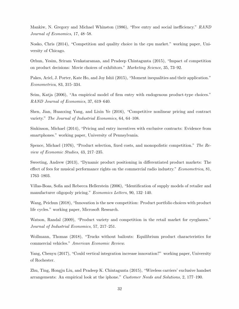
Mankiw, N. Gregory and Michael Whinston (1986), “Free entry and social inefficiency.” RAND

Journal of Economics, 17, 48–58.

Nosko, Chris (2014), “Competition and quality choice in the cpu market.” working paper, Uni-

versity of Chicago.

Orhun, Yesim, Sriram Venkataraman, and Pradeep Chintagunta (2015), “Impact of competition

on product decisions: Movie choices of exhibitors.” Marketing Science, 35, 73–92.

Pakes, Ariel, J. Porter, Kate Ho, and Joy Ishii (2015), “Moment inequalities and their application.”

Econometrica, 83, 315–334.

Seim, Katja (2006), “An empirical model of firm entry with endogenous product-type choices.”

RAND Journal of Economics, 37, 619–640.

Shen, Jian, Huanxing Yang, and Lixin Ye (2016), “Competitive nonlinear pricing and contract

variety.” The Journal of Industrial Economics, 64, 64–108.

Sinkinson, Michael (2014), “Pricing and entry incentives with exclusive contracts: Evidence from

smartphones.” working paper, University of Pennsylvania.

Spence, Michael (1976), “Product selection, fixed costs, and monopolistic competition.” The Re-

view of Economic Studies, 43, 217–235.

Sweeting, Andrew (2013), “Dynamic product positioning in differentiated product markets: The

effect of fees for musical performance rights on the commercial radio industry.” Econometrica, 81,

1763–1803.

Villas-Boas, Sofia and Rebecca Hellerstein (2006), “Identification of supply models of retailer and

manufacturer oligopoly pricing.” Economics Letters, 90, 132–140.

Wang, Peichun (2018), “Innovation is the new competition: Product portfolio choices with product

life cycles.” working paper, Microsoft Research.

Watson, Randal (2009), “Product variety and competition in the retail market for eyeglasses.”

Journal of Industrial Economics, 57, 217–251.

Wollmann, Thomas (2018), “Trucks without bailouts: Equilibrium product characteristics for

commercial vehicles.” American Economic Review.

Yang, Chenyu (2017), “Could vertical integration increase innovation?” working paper, University

of Rochester.

Zhu, Ting, Hongju Liu, and Pradeep K. Chintagunta (2015), “Wireless carriers’ exclusive handset

arrangements: An empirical look at the iphone.” Customer Needs and Solutions, 2, 177–190.

32

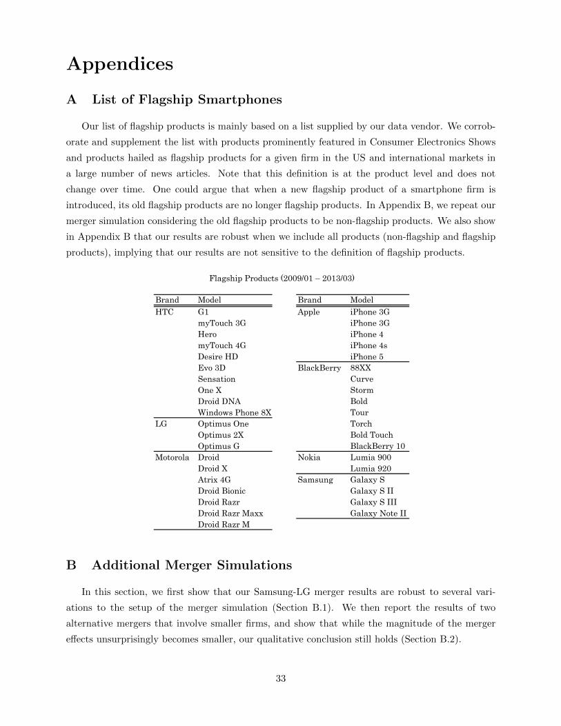
Appendices

A List of Flagship Smartphones

Our list of flagship products is mainly based on a list supplied by our data vendor. We corrob-

orate and supplement the list with products prominently featured in Consumer Electronics Shows

and products hailed as flagship products for a given firm in the US and international markets in

a large number of news articles. Note that this definition is at the product level and does not

change over time. One could argue that when a new flagship product of a smartphone firm is

introduced, its old flagship products are no longer flagship products. In Appendix B, we repeat our

merger simulation considering the old flagship products to be non-flagship products. We also show

in Appendix B that our results are robust when we include all products (non-flagship and flagship

products), implying that our results are not sensitive to the definition of flagship products.

Brand Model Brand ModelHTC G1 Apple iPhone 3G

myTouch 3G iPhone 3GHero iPhone 4myTouch 4G iPhone 4sDesire HD iPhone 5Evo 3D BlackBerry 88XXSensation CurveOne X StormDroid DNA BoldWindows Phone 8X Tour

LG Optimus One TorchOptimus 2X Bold TouchOptimus G BlackBerry 10

Motorola Droid Nokia Lumia 900Droid X Lumia 920Atrix 4G Samsung Galaxy SDroid Bionic Galaxy S IIDroid Razr Galaxy S IIIDroid Razr Maxx Galaxy Note IIDroid Razr M

Flagship Products (2009/01 – 2013/03)

B Additional Merger Simulations

In this section, we first show that our Samsung-LG merger results are robust to several vari-

ations to the setup of the merger simulation (Section B.1). We then report the results of two

alternative mergers that involve smaller firms, and show that while the magnitude of the merger

effects unsurprisingly becomes smaller, our qualitative conclusion still holds (Section B.2).

33

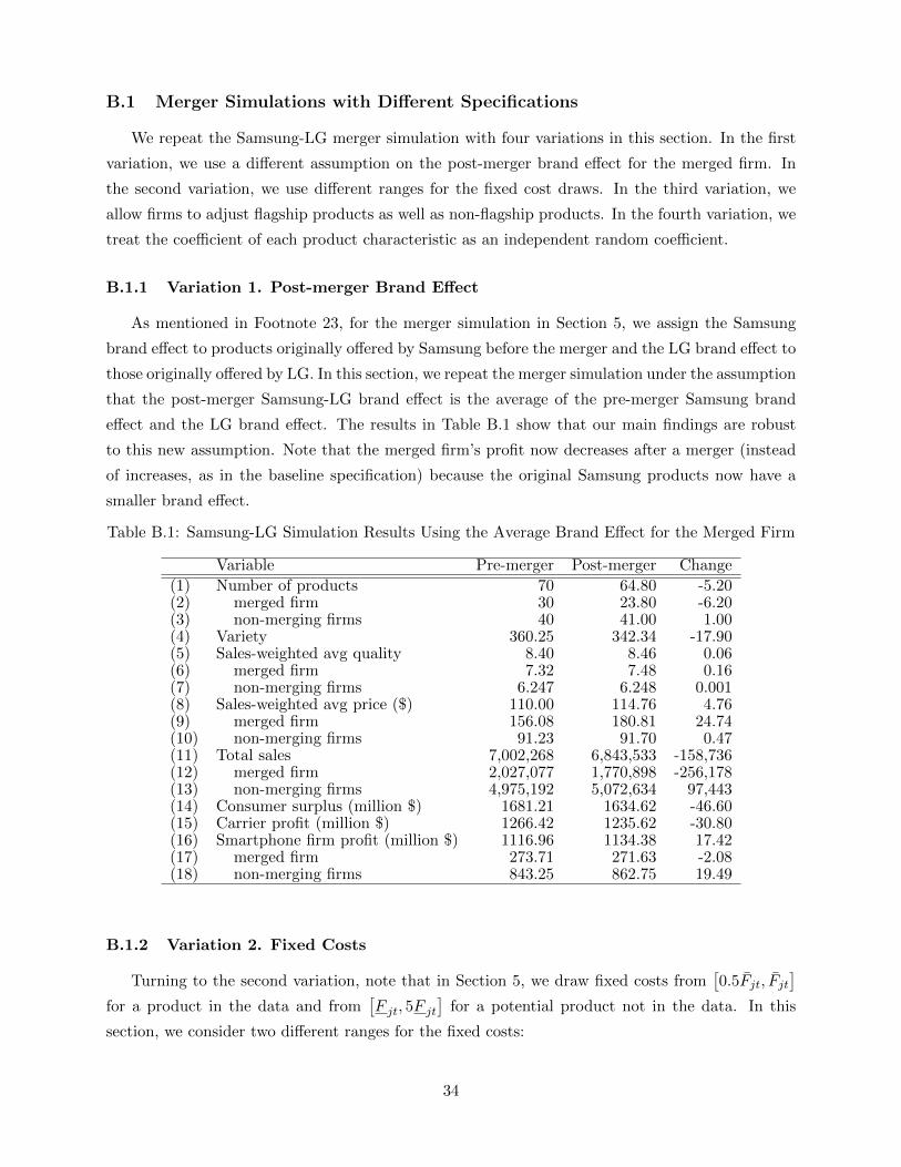
B.1 Merger Simulations with Different Specifications

We repeat the Samsung-LG merger simulation with four variations in this section. In the first

variation, we use a different assumption on the post-merger brand effect for the merged firm. In

the second variation, we use different ranges for the fixed cost draws. In the third variation, we

allow firms to adjust flagship products as well as non-flagship products. In the fourth variation, we

treat the coefficient of each product characteristic as an independent random coefficient.

B.1.1 Variation 1. Post-merger Brand Effect

As mentioned in Footnote 23, for the merger simulation in Section 5, we assign the Samsung

brand effect to products originally offered by Samsung before the merger and the LG brand effect to

those originally offered by LG. In this section, we repeat the merger simulation under the assumption

that the post-merger Samsung-LG brand effect is the average of the pre-merger Samsung brand

effect and the LG brand effect. The results in Table B.1 show that our main findings are robust

to this new assumption. Note that the merged firm’s profit now decreases after a merger (instead

of increases, as in the baseline specification) because the original Samsung products now have a

smaller brand effect.

Table B.1: Samsung-LG Simulation Results Using the Average Brand Effect for the Merged Firm

Variable Pre-merger Post-merger Change

(1) Number of products 70 64.80 -5.20(2) merged firm 30 23.80 -6.20(3) non-merging firms 40 41.00 1.00(4) Variety 360.25 342.34 -17.90(5) Sales-weighted avg quality 8.40 8.46 0.06(6) merged firm 7.32 7.48 0.16(7) non-merging firms 6.247 6.248 0.001(8) Sales-weighted avg price ($) 110.00 114.76 4.76(9) merged firm 156.08 180.81 24.74(10) non-merging firms 91.23 91.70 0.47(11) Total sales 7,002,268 6,843,533 -158,736(12) merged firm 2,027,077 1,770,898 -256,178(13) non-merging firms 4,975,192 5,072,634 97,443(14) Consumer surplus (million $) 1681.21 1634.62 -46.60(15) Carrier profit (million $) 1266.42 1235.62 -30.80(16) Smartphone firm profit (million $) 1116.96 1134.38 17.42(17) merged firm 273.71 271.63 -2.08(18) non-merging firms 843.25 862.75 19.49

B.1.2 Variation 2. Fixed Costs

Turning to the second variation, note that in Section 5, we draw fixed costs from[0.5F̄jt, F̄jt

]for a product in the data and from

[F jt, 5F jt

]for a potential product not in the data. In this

section, we consider two different ranges for the fixed costs:

34

(1)[F̄jt − (F̄ − F ), F̄jt

]for a product in the data and

[F jt, F jt + (F̄ − F )

]for a potential product

not in the data, where F̄ = 6.16 and F = 5.27 are, respectively, the average upper bound and

the average lower bound reported in Section 4.

(2)[F̄jt − (Lu(qjt)− Ll(qjt)), F̄jt

]for a product in the data and

[F jt, F jt + (Lu(qjt)− Ll(qjt))

]for a potential product not in the data, where Lu(qjt) = b̂u0+b̂u1qjt and (b̂u0, b̂u1) are obtained

by regressing the upper bounds reported in Section 4 on quality, and Ll(qjt) is analogously

defined using the lower bounds reported.

In Table B.2, we show that the merger simulation results are robust to these two alternative

fixed-cost ranges.

Table B.2: Samsung-LG Simulation Results Using Different Ranges for Fixed-cost Draws

Variable Pre-merger Post-merger Change

Alternative Fixed-cost Range (1)

(1) Number of products 70 67.20 -2.80

(2) merged firm 30 24.00 -6.00

(3) non-merging firms 40 43.20 3.20

(4) Variety 360.25 341.39 -18.86

(5) Sales-weighted avg quality 8.40 8.42 0.02

(6) merged firm 7.32 7.36 0.04

(7) non-merging firms 6.247 6.242 -0.005

(8) Sales-weighted avg price ($) 110.00 110.02 0.02

(9) merged firm 156.08 165.63 9.55

(10) non-merging firms 91.23 90.51 -0.72

(11) Total sales 7,002,268 6,896,415 -105,853

(12) merged firm 2,027,077 1,791,381 -235,695

(13) non-merging firms 4,975,192 5,105,034 129,842

(14) Consumer surplus (million $) 1681.21 1646.14 -35.07

(15) Carrier profit (million $) 1266.42 1247.78 -18.64

(16) Smartphone firm profit (million $) 1081.42 1097.88 16.46

(17) merged firm 252.96 255.12 2.15

(18) non-merging firms 828.46 842.76 14.30

Alternative Fixed-cost Range (2)

(1) Number of products 70 67.40 -2.60

(2) merged firm 30 24.60 -5.40

(3) non-merging firms 40 42.80 2.80

(4) Variety 360.25 342.48 -17.76

(5) Sales-weighted avg quality 8.40 8.42 0.02

(6) merged firm 7.32 7.36 0.04

(7) non-merging firms 6.247 6.242 -0.005

(8) Sales-weighted avg price ($) 110.00 110.40 0.40

(9) merged firm 156.08 166.30 10.22

(10) non-merging firms 91.23 90.57 -0.66

(11) Total sales 7,002,268 6,901,179 -101,089

(12) merged firm 2,027,077 1,807,624 -219,452

(13) non-merging firms 4,975,192 5,093,555 118,363

(14) Consumer surplus (million $) 1681.21 1647.85 -33.37

35

(15) Carrier profit (million $) 1266.42 1248.73 -17.69

(16) Smartphone firm profit (million $) 1084.76 1099.94 15.17

(17) merged firm 254.73 256.51 1.78

(18) non-merging firms 830.03 843.43 13.39

B.1.3 Variation 3. Allowing for Adjusting Flagship Products

In the baseline merger simulation, we only allow firms to adjust their non-flagship products.

We now add more products into consideration. Specifically, we first allow firms to also adjust old

flagship products (i.e., flagship products that are no longer at the quality frontier of a smartphone

firm) in Column (1) of Table B.3, and then in Column (2), we allow firms to adjust all products.

We find that both results are close to the baseline results.

Table B.3: Samsung-LG Simulation Results Allowing Adjusting Flagship Products

Variable Change

(1) Old Flagship (2) All FlagshipProducts Included Products Included

(1) Number of products -2.60 -2.60(2) merged firm -3.40 -3.40(3) non-merging firms 0.80 0.80(4) Variety -21.31 -24.00(5) Sales-weighted avg quality 0.02 0.02(6) merged firm 0.02 0.01(7) non-merging firms 0.0003 -0.001(8) Sales-weighted avg price ($) 1.42 0.82(9) merged firm 8.87 7.48(10) non-merging firms 0.27 0.22(11) Total sales -87,657 -95,193(12) merged firm -151,913 -171,627(13) non-merging firms 64,256 76,434(14) Consumer surplus (million $) -28.16 -31.41(15) Carrier profit (million $) -16.60 -15.45(16) Smartphone firm profit (million $) 13.41 13.70(17) merged firm 1.75 1.66(18) non-merging firms 11.66 12.05

B.1.4 Variation 4. Independent Random Coefficients

In our baseline specification, we assume that the utility of a consumer depends on the product

characteristics through a quality index. In other words, the random coefficient for each product

characteristic is perfectly correlated. Specifically, the random coefficient for characteristic k is

(β + σµi)θk. In this robustness analysis, we repeat the merger simulation allowing the random

coefficient to be independent across k, i.e., to be (β + σµki)θk where µ1i, ..., µKi are independent

random variables, and β, σ and θk are the estimates reported in Section 4. We re-estimate the

supply-side parameters. Table B.4 shows that our merger simulation results are robust to this

variation.

36

Table B.4: Samsung-LG Simulation Results Assuming Independent Random Coefficients

Variable Pre-merger Post-merger Change

(1) Number of products 70 66.80 -3.20(2) merged firm 30 21.80 -4.20(3) non-merging firms 40 29.00 1.00(4) Variety 94.83 91.93 -2.91(5) Sales-weighted avg quality 5.82 5.85 0.03(6) merged firm 5.06 5.09 0.03(7) non-merging firms 4.082 4.082 0.001(8) Sales-weighted avg price ($) 72.91 76.88 3.97(9) merged firm 52.78 61.20 8.43(10) non-merging firms 88.15 87.72 -0.43(11) Total sales 7,192,967 7,055,617 -137,351(12) merged firm 3,099,041 2,883,673 -215,368(13) non-merging firms 4,093,927 4,171,944 78,017(14) Consumer surplus (million $) 1515.24 1478.08 -37.16(15) Carrier profit (million $) 1265.09 1239.79 -25.29(16) Smartphone firm profit (million $) 1117.20 1129.91 12.71(17) merged firm 514.20 516.93 2.73(18) non-merging firms 602.99 612.97 9.98

B.2 Samsung-Motorola Merger and LG-Motorola Merger

In Section 5, we have shown the simulation result for a merger between Samsung and LG in

March 2013, the second and third largest firms in terms of sales in that month. In this section,

we conduct two additional merger simulations: a Samsung-Motorola merger (a merger between the

second-largest and the fourth-largest firms) and an LG-Motorola merger (a merger between the

third-largest and the fourth-largest firms). The simulation results are presented in Table B.5. A

comparison of the results in Table 9 for the Samsung-LG merger to the results here shows that, not

surprisingly, the merger effects on product offerings and welfare are smaller for mergers between

smaller firms. However, the qualitative findings are robust. Specifically, we find that all three

mergers lead to a decrease in product variety. In terms of welfare, all three mergers result in a

decrease in both consumer and carrier surplus, but an increase in smartphone producer surplus.

The overall welfare effect is always negative.

C Additional Robustness Analyses

In this appendix, we investigate whether our results are robust to additional variations to the

demand side and the supply side of the model (in addition to those considered in Section 6). We

also estimate a parametric fixed cost function which allows for potential economies or diseconomies

of scope in fixed costs.

37

Table B.5: Results from Additional Merger Simulations, March 2013

Variable Pre-merger Post-merger Change

The Samsung-Motorola Merger

(1) Number of products 70 67.80 -2.20(2) merged firm 25 22.60 -2.40(3) non-merging firms 45 45.20 0.20(4) Variety 360.25 350.65 -9.60(5) Sales-weighted avg quality 8.401 8.416 0.015(6) merged firm 7.359 7.359 0.000(7) non-merging firms 6.245 6.246 0.001(8) Sales-weighted avg price ($) 110.00 110.36 0.35(9) merged firm 161.32 166.03 4.71

(10) non-merging firms 89.91 90.21 0.29(11) Total sales 7,002,268 6,927,079 -75,189(12) merged firm 1,970,007 1,840,880 -129,127(13) non-merging firms 5,032,261 5,086,199 53,938(14) Consumer surplus (million $) 1681.21 1656.47 -24.74(15) Carrier profit (million $) 1266.42 1249.10 -17.32(16) Smartphone firm profit (million $) 1116.96 1130.92 13.96(17) merged firm 275.90 277.88 1.98(18) non-merging firms 841.06 853.04 11.97

The LG-Motorola Merger

(1) Number of products 70 69.40 -0.60(2) merged firm 19 18.40 -0.60(3) non-merging firms 51 51.00 0.00(4) Variety 360.25 357.14 -3.10(5) Sales-weighted avg quality 8.401 8.407 0.005(6) merged firm 7.106 7.090 -0.016(7) non-merging firms 6.495 6.496 0.0004(8) Sales-weighted avg price ($) 110.00 110.12 0.12(9) merged firm 144.92 146.75 1.82

(10) non-merging firms 105.99 106.14 0.14(11) Total sales 7,002,268 6,980,382 -21,886(12) merged firm 721,570 682,979 -38,591(13) non-merging firms 6,280,699 6,297,403 16,705(14) Consumer surplus (million $) 1681.21 1674.08 -7.13(15) Carrier profit (million $) 1266.42 1261.37 -5.05(16) Smartphone firm profit (million $) 1116.96 1121.47 4.52(17) merged firm 59.68 59.85 0.17(18) non-merging firms 1057.28 1061.62 4.34

38

C.1 Alternative Demand Specifications

We replace the brand fixed effects by the brand/year fixed effects in one robustness analysis,

and include the age of a product (i.e., how long a product has been in the market) and the square

of it in the other robustness analysis. Our results are again robust (see Tables C.1 and C.2).

C.2 Alternative Pricing Models

On the supply side, we have shown in Section 6 that our results are robust to an alternative

pricing model, where Apple and AT&T jointly set the retail prices for iPhones before their exclusive

contract expired. In this section, we consider another three alternative pricing models.

Note that the simple linear pricing model in the baseline specification implies that there exists

double marginalization as follows:

p = (−Γc ◦∆c)−1 s+ (−Γm ◦∆m)−1 s+ m̃c, (C.1)

where the operator ◦ represents the element-wise multiplicity, and Γc is a matrix whose (i, j) element

= 1 if products i and j are sold by the same carrier, and 0 otherwise. Analogously, Γm is a matrix

whose (i, j) element = 1 if and only if products i and j are produced by the same smartphone

firm. While Γc and Γm describe the “ownership,” the other two matrices, ∆c and ∆m, describe the

price sensitivity of demand. Specifically, the (i, j) element of ∆c and ∆m are, respectively,∂sj∂pi

and∑k∂sj∂pk

∂p∗k∂wi

.

As pointed out by Villas-Boas and Hellerstein (2006), it is possible that the pricing strategies of

smartphone firms and/or carriers deviate from a linear pricing model. Villas-Boas and Hellerstein

(2006) introduce two vectors Λc and Λm to capture such deviations so that the following equation

describes the pricing behavior:

p =[(−Γ̄c ◦∆c

)−1s]◦ Λc +

[(−Γ̄m ◦∆m

)−1s]◦ Λm + m̃c, (C.2)

where the “ownership” matrices Γ̄c and Γ̄m can also deviate from those in the simple linear pricing

model (i.e., Γc and Γm).

The baseline model is a case where Λc and Λm are both constant-1 vectors and (Γ̄c = Γc,

Γ̄m = Γm). With a slight abuse of notation, we refer to this case as (Λc = 1,Λm = 1, Γ̄c = Γc, Γ̄m =

Γm). The Apple and AT&T joint price setting model we studied in Section 6 is a case where

Λc = 1, Γ̄m = Γm, and

Λm (j) =

{1 if j ∈ same non-Apple smartphone firm

0 otherwise(C.3)

Γ̄c (i, j) =

{1 if i, j ∈ (iPhones) or (AT&T and non-iPhones) or (same non-AT&T carrier)

0 otherwise.

39

Table C.1: Robustness Analysis: Allowing Brand/Year Fixed Effects

(a) Estimation Results

Parameter Std. Error

Demand

Quality coefficientbattery talk time (hours) 0.056∗∗∗ 0.015camera resolution (megapixel) 0.092∗∗ 0.041chipset generation 2 0.538∗∗∗ 0.146chipset generation 3 0.840∗∗∗ 0.199chipset generation 4 1.142∗∗∗ 0.276chipset generation 5 1.811∗∗∗ 0.375screen size (inch) 1weight (gram) -0.003∗∗ 0.002

Covariance of random coefficientsmean 0.530∗∗∗ 0.139std. dev. 0.340∗∗∗ 0.075

Price -0.003∗∗ 0.002Flagship? 0.663∗∗∗ 0.063Brand/year, carrier/year and quarter dummies Yes

Marginal Cost ($)

Exp(quality/10) 463.048∗∗∗ 2.397Apple -73.115∗∗∗ 0.128BlackBerry 89.889∗∗∗ 0.41Samsung -29.909∗∗∗ 0.131Carrier/year dummies Yes

* indicates 90% level of significance. ** indicates 95% level of significance.*** indicates 99% level of significance.

(b) Welfare Changes when a Product is Removed, March 2013 (million $)

Removed product Lowest-quality Median Highest

∆(consumer surplus) -0.67 -3.89 -25.45∆(carrier surplus) -0.50 -2.15 -17.92∆(smartphone producer variable profits) -0.36 -1.70 -2.22Upper bound of savings in fixed costs 0.63 3.45 22.10

(c) Welfare Changes when a Product is Added, March 2013 (million $)

HTC LG Motorola Samsung

∆(consumer surplus) 2.36 4.19 2.37 4.22∆(carrier surplus) 1.18 1.8 1.19 1.82∆(smartphone producer variable profits) 0.81 1.14 0.8 1.12lower bound of added fixed costs 1.92 3.23 1.93 3.25

(d) The Effect of Samsung-LG Merger in March 2013

Variable Pre-merger Post-merger Change

Number of products 70 67.40 -2.60Variety 453.04 440.08 -12.97Sales-weighted avg quality 10.19 10.23 0.04Sales-weighted avg price ($) 162.58 166.87 4.29Total sales 7,433,790 7,355,555 -78,235Consumer surplus (million $) 3704.08 3650.28 -53.80Carrier profit (million $) 2650.87 2624.67 -26.19Smartphone firm profit (million $) 2594.51 2622.01 27.50

40

Table C.2: Robustness Analysis: Allowing Age in the Utility Function

(a) Estimation Results

Parameter Std. Error

Demand

Quality coefficientbattery talk time (hours) 0.046∗∗∗ 0.013camera resolution (megapixel) 0.091∗∗∗ 0.036chipset generation 2 0.240∗∗∗ 0.100chipset generation 3 0.344∗∗∗ 0.131chipset generation 4 0.461∗∗∗ 0.185chipset generation 5 0.594∗∗ 0.260screen size (inch) 1weight (gram) 0.0004 0.002

Covariance of random coefficientsmean 0.802∗∗∗ 0.146std. dev. 0.291∗∗∗ 0.093

Price -0.238∗∗∗ 0.078Apple 3.121∗∗∗ 0.113BlackBerry 1.233∗∗∗ 0.117Samsung 0.403∗∗∗ 0.070Flagship? 0.911∗∗∗ 0.081Age -0.292∗∗∗ 0.037Age2 0.013∗∗∗ 0.003Carrier/year and quarter dummies Yes

Marginal Cost ($)

Exp(quality/10) 724.827∗∗∗ 2.988Apple -13.431∗∗∗ 0.108BlackBerry 119.201∗∗∗ 0.458Samsung -18.228∗∗∗ 0.122Carrier/year dummies Yes

* indicates 90% level of significance. ** indicates 95% level of significance.*** indicates 99% level of significance.

(b) Welfare Changes when a Product is Removed, March 2013 (million $)

Removed product Smallest ∆(CS) Median Largest

∆(consumer surplus) -1.08 -3.36 -10.78∆(carrier surplus) -0.56 -1.66 -6.01∆(smartphone producer variable profits) -0.38 -1.23 -5.41Upper bound of savings in fixed costs 0.88 2.79 9.83

(c) Welfare Changes when a Product is Added, March 2013 (million $)

HTC LG Motorola Samsung

∆(consumer surplus) 4.11 3.84 4.11 3.84∆(carrier surplus) 2.38 1.99 2.4 2.01∆(smartphone producer variable profits) 1.9 1.52 1.89 1.51lower bound of added fixed costs 3.61 3.23 3.62 3.24

(d) The Effect of Samsung-LG Merger in March 2013

Variable Pre-merger Post-merger Change

Number of products 70 67.80 -2.20Variety 310.41 294.20 -16.21Sales-weighted avg quality 7.96 7.98 0.02Sales-weighted avg price ($) 76.03 77.16 1.13Total sales 7,854,756 7,793,287 -61,469Consumer surplus (million $) 1296.58 1283.22 -13.36Carrier profit (million $) 1027.46 1019.91 -7.55Smartphone firm profit (million $) 923.87 929.87 6.00

41

We now consider three alternative deviations from the baseline model:

Additional Case 1. In this case, smartphone manufacturers decide the retail prices directly.

Smartphone firm m’s profit maximization problem is:

maxpj ,j∈Jm

∑j∈Jm

(pj − m̃cj) sj (p) . (C.4)

The first-order condition is equivalent to (C.2) where (Λc = 0,Λm = 1, Γ̄c = Γc, Γ̄m = Γm).28

Additional Case 2. In this case, carriers choose the retail prices while facing a wholesale price

that equals the marginal cost of each product. In other words, carrier c’s profit maximization

problem is:

maxpj ,j∈Jc

∑j∈Jc

(pj − m̃cj) sj (p) . (C.5)

The first-order condition is equivalent to (C.2) where (Λc = 1,Λm = 0, Γ̄c = Γc, Γ̄m = Γm).

Additional Case 3. In this case, all smartphones and all carriers jointly set retail prices. Specifi-

cally, we consider each smartphone firm/carrier pair (m, c) to jointly solve the following maximiza-

tion problem:

maxpj ,j∈Jmc

∑j∈Jmc

Πj (p)︸ ︷︷ ︸pair (m,c)’s profit

+ µm∑

j∈Jm,j 6∈Jc

τΠj (p)︸ ︷︷ ︸firm m’s profit from other products

+ µc∑

j∈Jc,j 6∈Jm

(1− τ) Πj (p)︸ ︷︷ ︸carrier c’s profit from other products

, (C.6)

where Πj (p) = (pj − m̃cj) sj (p) is the joint profit from selling product j, the parameter τ is the

share of profit that goes to a smartphone firm (and thus 1 − τ is the share for a carrier), and µm

and µc are, respectively, the weights that the smartphone firm/carrier pair puts on the smartphone

firm’s profit from selling other products and the carrier’s profit from selling other products. This

model is therefore equivalent to Λc = 1,Λm = 0, and

Γ̄c (i, j) =

1 if i, j ∈ same smartphone firm/carrier,

µmτ if i, j ∈ same smartphone firm, but different carriers,

µc (1− τ) if i, j ∈ same carrier, but different smartphone firms,

0 otherwise.

(C.7)

In what follows, we discuss these three additional robustness analyses. Specifically, we re-

estimate the marginal cost parameters and the bounds on the fixed costs and repeat our coun-

terfactual simulations. For simplicity of exposition, we suppress the subscript “t” and ignore the

distinction between j and j̃.

28In this case, the (i, j) element of ∆m is∂sj∂pi

.

42

Additional Case 1

In this case, the per-unit profit for a carrier is zero and there should be a transfer from a

smartphone firm to a carrier. Let Tm be the total transfer that a smartphone firm m pays, Tm,\j be

the transfer when product j is removed from m’s product portfolio and Tm,∪j be the transfer when

product j is added to m’s product portfolio. Then, the two inequalities (11) and (12) in Section 3,

which capture the optimal conditions for m’s product choice in the baseline model, become:

E(ξ,η)πm (q, ξ,η)− Fj − Tm ≥ E(ξ\ξj ,η\ηj)πm (q\qj , ξ\ξj ,η\ηj)− Tm,\j for any j ∈ Jm (C.8)

E(ξ,η)πm (q, ξ,η)− Tm ≥ E(ξ∪ξj ,η∪ηj)πm (q ∪ qj , ξ ∪ ξj ,η ∪ ηj)− Fj − Tm,∪j for any j 6∈ Jm.

The two inequalities in (C.8) imply that for any j ∈ Jm,

Fj ≤[E(ξ,η)πm (q, ξ,η)− E(ξ\ξj ,η\ηj)πm (q\qj , ξ\ξj ,η\ηj)

]−[Tm − Tm,\j

](C.9)

, ∆πm,\j −[Tm − Tm,\j

], F̄j ,

and for any j 6∈ Jm,

Fj ≥[E(ξ∪ξj ,η∪ηj)πm (q ∪ qj , ξ ∪ ξj ,η ∪ ηj)− E(ξ,η)πm (q, ξ,η)

]− [Tm,∪j − Tm] (C.10)

, ∆πm,∪j − [Tm,∪j − Tm] , F j .

These transfers do not affect the equilibrium prices. Therefore, they do not affect consumer

surplus or the sum of carriers’ variable profit and smartphone firms’ variable profits. They do,

however, affect our estimates of the fixed cost bounds (see (C.9) and (C.10)). We argue that under

a reasonable assumption on the transfers, we can obtain an overestimate of the bounds without

modeling how the transfers are determined. Specifically, the assumption we need is: the total

transfer that a smartphone pays at least weakly increases with the number of its products, i.e.,

Assumption 1 Tm − Tm,\j ≥ 0 and Tm,∪j − Tm ≥ 0.

Under Assumption 1, we have F̄j ≤ ∆πm,\j and F j ≤ ∆πm,∪j . We think this assumption is

reasonable, in other words, we expect the upper bound (or the lower bound) to be smaller than

∆πm,\j (or ∆πm,∪j). For example, if a carrier shares a portion (denoted by ϕ ∈ (0, 1)) of the

increase in a smartphone firm’s variable profit when a product is added, i.e., Tm−Tm,\j = ϕ∆πm,\j

and Tm,∪j−Tm = ϕ∆πm,∪j , then F̄j = (1−ϕ)∆πm,\j < ∆πm,\j and F j = (1−ϕ)∆πm,∪j < ∆πm,∪j .

In Table C.3 where we present the simulation results when a product is removed or added, we

report these overestimated bounds: ∆πm,\j and ∆πm,∪j . Table C.3 shows that even with such

an overestimation, our results are robust: removing a product leads to a decrease in total welfare

even considering the (over-estimated) maximum possible saving in the fixed cost while adding a

product leads to an increases in the total welfare as long as the fixed cost of the added product

43

is not much higher than its (over-estimated) lower bound. In sum, our results on welfare changes

when a product is added or removed are robust to this change to the supply side of the model.29

Table C.3: Robustness Test, Λc = 0,Λm = 1, Γ̄m = Γm

(a) Welfare Changes when a Product is Removed, March 2013 (million $)

Removed product Lowest-quality Median Highest

∆(consumer surplus) -1.03 -2.28 -13.98∆(total producer surplus net of fixed costs)a -0.59 -0.83 -3.93∆πm,\j 0.97 2.03 12.17aThe sum of carriers’ variable profits and smartphone firms’ variable profits.

(b) Welfare Changes when a Product is Added, March 2013 (million $)

HTC LG Motorola Samsung

∆(consumer surplus) 2.35 2.40 2.40 2.71∆(total producer surplus net of fixed costs) 1.02 0.99 0.99 1.69∆πm,∪j 2.14 2.17 2.17 2.70

Additional Case 2

In this case, the transfer should be from a carrier to a smartphone instead. Let Tm be the total

transfer that a smartphone firm m receives, and Tm,\j and Tm,∪j be that when j is removed from

or when j is added to m’s product portfolio. Then, the two inequalities (11) and (12) become:

Tm − Fj ≥ Tm,\j ⇐⇒ Fj ≤ Tm − Tm,\j for any j ∈ Jm (C.11)

Tm ≥ Tm,∪j − Fj ⇐⇒ Fj ≥ Tm,∪j − Tm for any j 6∈ Jm. (C.12)

We again make an assumption on the transfers. Specifically, let the changes in the (pre-transfer)

profit of j’s carrier be:

∆πc,\j = E(ξ,η)πc (q, ξ,η)− E(ξ\ξj ,η\ηj)πc (q\qj , ξ\ξj ,η\ηj) , (C.13)

∆πc,∪j = E(ξ∪ξj ,η∪ηj)πc (q ∪ qj , ξ ∪ ξj ,η ∪ ηj)− E(ξ,η)πc (q, ξ,η) .

We assume that the increase in the amount of transfer that the smartphone firm receives is not

larger than the increase in the carrier’s (pre-transfer) profit, i.e.,

Assumption 2 Tm − Tm,\j ≤ ∆πc,\j and Tm,∪j − Tm ≤ ∆πc,∪j.

In Table C.4, which presents the simulation results in this robustness analysis, we report ∆πc,\j

in Table C.4(a) and ∆πc,∪j in Table C.4(b). Under Assumption 2, the bounds of the fixed cost

29We do not conduct robustness analyses regarding the merger simulations because doing so requires us to makeassumptions on how large the transfer from each smartphone firm to each carrier is and how a merger affects thetransfers between smartphone firms and carriers.

44

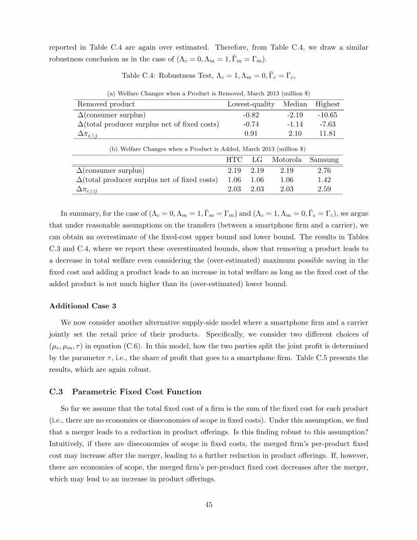
reported in Table C.4 are again over estimated. Therefore, from Table C.4, we draw a similar

robustness conclusion as in the case of (Λc = 0,Λm = 1, Γ̄m = Γm).

Table C.4: Robustness Test, Λc = 1,Λm = 0, Γ̄c = Γc,

(a) Welfare Changes when a Product is Removed, March 2013 (million $)

Removed product Lowest-quality Median Highest

∆(consumer surplus) -0.82 -2.19 -10.65∆(total producer surplus net of fixed costs) -0.74 -1.14 -7.63∆πc,\j 0.91 2.10 11.81

(b) Welfare Changes when a Product is Added, March 2013 (million $)

HTC LG Motorola Samsung

∆(consumer surplus) 2.19 2.19 2.19 2.76∆(total producer surplus net of fixed costs) 1.06 1.06 1.06 1.42∆πc,∪j 2.03 2.03 2.03 2.59

In summary, for the case of (Λc = 0,Λm = 1, Γ̄m = Γm) and (Λc = 1,Λm = 0, Γ̄c = Γc), we argue

that under reasonable assumptions on the transfers (between a smartphone firm and a carrier), we

can obtain an overestimate of the fixed-cost upper bound and lower bound. The results in Tables

C.3 and C.4, where we report these overestimated bounds, show that removing a product leads to

a decrease in total welfare even considering the (over-estimated) maximum possible saving in the

fixed cost and adding a product leads to an increase in total welfare as long as the fixed cost of the

added product is not much higher than its (over-estimated) lower bound.

Additional Case 3

We now consider another alternative supply-side model where a smartphone firm and a carrier

jointly set the retail price of their products. Specifically, we consider two different choices of

(µc, µm, τ) in equation (C.6). In this model, how the two parties split the joint profit is determined

by the parameter τ , i.e., the share of profit that goes to a smartphone firm. Table C.5 presents the

results, which are again robust.

C.3 Parametric Fixed Cost Function

So far we assume that the total fixed cost of a firm is the sum of the fixed cost for each product

(i.e., there are no economies or diseconomies of scope in fixed costs). Under this assumption, we find

that a merger leads to a reduction in product offerings. Is this finding robust to this assumption?

Intuitively, if there are diseconomies of scope in fixed costs, the merged firm’s per-product fixed

cost may increase after the merger, leading to a further reduction in product offerings. If, however,

there are economies of scope, the merged firm’s per-product fixed cost decreases after the merger,

which may lead to an increase in product offerings.

45

Table C.5: Robustness Test: Smartphone Firm/Carrier Pairs Joint Price Setting

(a) (µc = 0, µm = 0)a

(a.1) Welfare Changes when a Product is Removed, March 2013 (million $)

Removed product Lowest-quality Median Highest

∆(consumer surplus) -0.85 -1.87 -10.93∆(total producer surplus net of fixed costs) -0.56 -0.86 -4.60Upper bound of savings in fixed costs 0.41 0.87 5.26

(a.2) Welfare Changes when a Product is Added, March 2013 (million $)

HTC LG Motorola Samsung

∆(consumer surplus) 1.94 1.93 1.96 2.50∆(total producer surplus net of fixed costs) 0.96 0.96 0.96 1.34Lower bound of added fixed costs 0.90 0.91 0.91 1.08aIn this case, the value of τ is irrelevant.

(b) (µc = 0.5, µm = 0.5, τ = 0.5)

(b.1) Welfare Changes when a Product is Removed, March 2013 (million $)

Removed product Lowest-quality Median Highest

∆(consumer surplus) -0.82 -1.90 -10.90∆(total producer surplus net of fixed costs) -0.58 -0.88 -4.98Upper bound of savings in fixed costs 0.42 0.91 5.56

(b.2) Welfare Changes when a Product is Added, March 2013 (million $)

HTC LG Motorola Samsung

∆(consumer surplus) 1.95 1.96 1.97 2.43∆(total producer surplus net of fixed costs) 0.96 0.96 0.96 1.38Lower bound of added fixed costs 0.91 0.93 0.92 1.11

To address this concern, we now take a parametric approach and specify a function of the fixed

cost allowing for economies or diseconomies of scope as follows:

FCjt = φ1qj + φ2 log(nm(j)t

)+ ϕm(j)t, (C.14)

where qj is product j’s quality index, nm(j)t is the number of products that the smartphone firm

m(j) has in period t, and ϕm(j)t represents the brand/time fixed effects.30 Note that a negative

estimate of the coefficient φ2 indicates economies of scope in fixed costs; and conversely, a positive

estimate indicates diseconomies of scope.

Note that the purpose of this exercise is to address the concern that potential economies of scope

in fixed costs may lead to an increase in the number of products after a merger, which would be

the opposite of our baseline results. Therefore, our goal in this section is to obtain a (conservative)

estimate of the lower bound for φ2. If our conservative estimate of the lower bound is positive (or

30For notational simplicity, we use j instead of j̃ to represent a product, i.e., we ignore the distinction between jand j̃ as explained in Section 3.2.2.

46

negative but of small magnitude), then we can conclude that there are diseconomies of scope (or

small economies of scope) in fixed costs.

To obtain the estimate of the lower bound for φ2, we consider the following three types of

deviations:

(1) Dropping a product j

Nash equilibrium implies that dropping a product does not increase the expected profit of a

firm. Let Πmt (Jmt) = E(ξt,ηt)πmt (qt, ξt,ηt) be the expected profit that a smartphone firm m gets

from its observed product portfolio Jmt and Πmt (Jmt\ j) = E(ξt\ξjt,ηt\ηjt)πmt (qt\qj , ξt\ξjt,ηt\ηjt)be that when it drops product j. Then, for any j ∈ Jmt,

[Πmt (Jmt)− (φ1qj + ϕmt)− φ2nmt log (nmt)]−[Πmt (Jmt\ j)− φ2 (nmt − 1) log (nmt − 1)]+υjt ≥ 0,

where υjt is added to the inequality to represent an expectation error that is uncorrelated with

product choices (e.g., Holmes (2011) and Pakes, Porter, Ho and Ishii (2015)). Then,

φ1qj + ϕmt + φ2 [nmt log (nmt)− (nmt − 1) log (nmt − 1)] (C.15)

≤ Πmt (Jmt)−Πmt (Jmt\ j) + υjt.

(2) Replacing product j by a high-quality product j′

Such a deviation gives us the following inequality:

[Πmt (Jmt)− (φ1qj + ϕmt)− φ2nmt log (nmt)]

−[Πmt

(Jmt\ j ∪ j′

)−(φ1qj′ + ϕmt

)− φ2nmt log (nmt)

]+ υjj′t ≥ 0,

implying

φ1

(qj′ − qj

)≥ Πmt

(Jmt\ j ∪ j′

)−Πmt (Jmt)− υjj′t. (C.16)

(3) Replacing product j by two products k1 and k2 such that qk1 + qk2 = qj

Similarly, we have

[Πmt (Jmt)− (φ1qj + ϕmt)− φ2nmt log (nmt)]

− [Πmt (Jmt\ j ∪ k1 ∪ k2)− (φ1qk1 + ϕmt)− (φ1qk2 + ϕmt)− φ2 (nmt + 1) log (nmt + 1)] + υjk1k2t ≥ 0,

implying

ϕmt + φ2 [(nmt + 1) log (nmt + 1)− nmt log (nmt)] (C.17)

≥ Πmt (Jmt\ j ∪ k1 ∪ k2)−Πmt (Jmt)− υjk1k2t.

To obtain a conservative lower bound for φ2, we take the difference of (C.17) and (C.15) and

47

obtain

φ2 [(nmt + 1) log (nmt + 1)− 2nmt log (nmt) + nmt log (nmt)] (C.18)

≥ [Πmt (Jmt\ j ∪ k1 ∪ k2)−Πmt (Jmt)]− [Πmt (Jmt)−Πmt (Jmt\ j)] + φ1qj − υjt − υjk1k2t≥ [Πmt (Jmt\ j ∪ k1 ∪ k2)−Πmt (Jmt)]− [Πmt (Jmt)−Πmt (Jmt\ j)]

+Πmt (Jmt\ j ∪ j′)−Πmt (Jmt)

qj′ − qjqj − υjt − υjk1k2t −

qjqj′ − qj

υjj′t,

where the second inequality is obtained by plugging (C.16) into the first inequality. This inequality

eventually gives us

φ2 ≥[Πmt (Jmt\ j ∪ k1 ∪ k2)−Πmt (Jmt)]− [Πmt (Jmt)−Πmt (Jmt\ j)] + Πmt(Jmt\ j∪j′)−Πmt(Jmt)

qj′−qjqj

[(nmt + 1) log (nmt + 1)− 2nmt log (nmt) + nmt log (nmt)]

−−υjt − υjk1k2t −

qjqj′−qj

υjj′t

[(nmt + 1) log (nmt + 1)− 2nmt log (nmt) + nmt log (nmt)].

, Φjt + εjt, (C.19)

We denote the first line in (C.19) by Φjt, and with a slight abuse of notation, the second line by

εjt.31 As mentioned, we assume that εjt is uncorrelated with product choices. Then, we have

φ2 ≥ EΦjt. (C.20)

In estimation, we set the quality difference qj′ − qj in (C.16) to be 0.05, and qk1 = 0.4qj and

qk2 = 0.6qj in (C.17).32 According to our estimate, the lower bound of the estimated set for

φ2 is 1#J

∑jt∈J Φjt = 0.017. Following Imbens and Manski (2004), the lower bound of the 95%

confidence interval for φ2 is 1#J

∑jt∈J Φjt−

√v̂ar(Φjt)√

#J c0.05 = 0.016, where v̂ar(Φjt) is an estimator

of the variance of Φjt and c0.05 represents the critical value. These results suggest that there are

some diseconomies of scope in fixed costs. For example, φ2 = 0.017 means that, for the merged firm

Samsung-LG, when it drops a product, the fixed cost for each of its remaining products decreases

by 1.6 million dollars. Therefore, if anything, we underestimate the decrease in product offerings

in our baseline results.

31As will be explained later, in the estimation, we choose qj′ , qk1 and qk2 as a constant function of qj . As theresult, the second summand in (C.19) is only jt specific.

32The results are robust to other choices of qj′ − qj and (qk1, qk2).

48

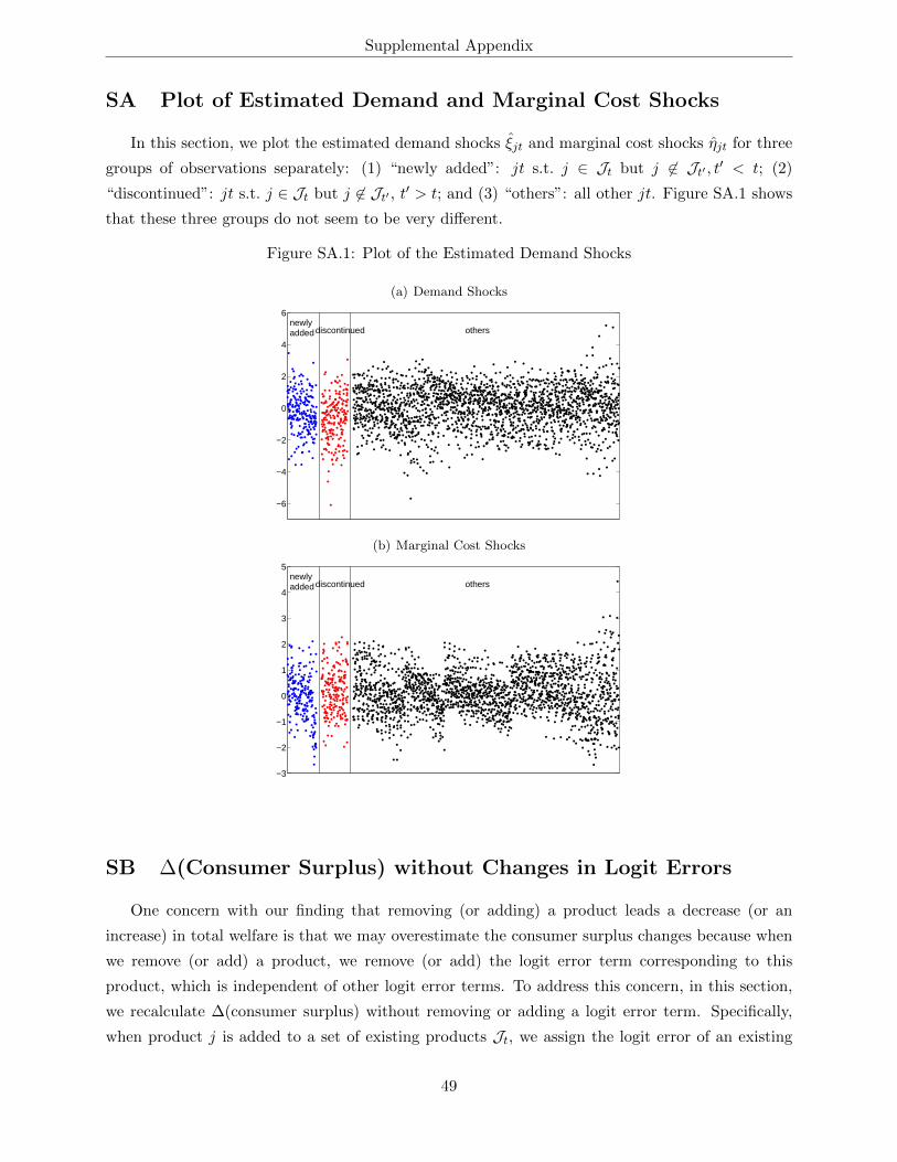
Supplemental Appendix

SA Plot of Estimated Demand and Marginal Cost Shocks

In this section, we plot the estimated demand shocks ξ̂jt and marginal cost shocks η̂jt for three

groups of observations separately: (1) “newly added”: jt s.t. j ∈ Jt but j 6∈ Jt′ , t′ < t; (2)

“discontinued”: jt s.t. j ∈ Jt but j 6∈ Jt′ , t′ > t; and (3) “others”: all other jt. Figure SA.1 shows

that these three groups do not seem to be very different.

Figure SA.1: Plot of the Estimated Demand Shocks

(a) Demand Shocks

−6

−4

−2

0

2

4

6newlyaddeddiscontinued others

(b) Marginal Cost Shocks

−3

−2

−1

0

1

2

3

4

5newlyaddeddiscontinued others

SB ∆(Consumer Surplus) without Changes in Logit Errors

One concern with our finding that removing (or adding) a product leads a decrease (or an

increase) in total welfare is that we may overestimate the consumer surplus changes because when

we remove (or add) a product, we remove (or add) the logit error term corresponding to this

product, which is independent of other logit error terms. To address this concern, in this section,

we recalculate ∆(consumer surplus) without removing or adding a logit error term. Specifically,

when product j is added to a set of existing products Jt, we assign the logit error of an existing

49

Supplemental Appendix

product k ∈ Jt to the added product j so that there is no added logit error term. We choose

product k to be the closest to j’s quality among all existing products of j’s manufacturer.33 We

take a similar approach for the case of removing a product. Note that when product j is removed

from the set Jt, the decrease in consumer surplus is essentially the increase in consumer surplus

when product j is added to the set Jt\j.With this alternative measure of consumer surplus, Tables 7 (removing a product) and 8 (adding

a product) become:

Table SB.1: Welfare Changes When a Product Is Removed, March 2013 (million $)

Removed product Lowest-quality Median Highest

∆(consumer surplus without changes in logit errors) -0.46 -1.51 -10.35∆(carrier surplus) -0.83 -1.39 -9.13∆(smartphone producer variable profits) -0.50 -0.90 -3.24Upper bound of savings in fixed costs 0.94 2.19 12.14

Rows 1+2+3+4 -0.45 -0.54 -8.12

Table SB.2: Welfare Changes When a Product Is Added, March 2013 (million $)

HTC LG Motorola Samsung

∆(consumer surplus without changes in logit errors) 1.11 1.26 1.38 2.09∆(carrier surplus) 1.26 1.27 1.29 1.53∆(smartphone producer variable profits) 1.04 1.03 1.00 1.64Lower bound of added fixed costs 2.10 2.11 2.13 2.62

(Rows 1+2+3)/(Row 4) 1.62 1.69 1.72 2.01

The changes in consumer surplus are indeed smaller than what are reported in Tables 7 and 8.

However, the sum of the four rows in Table SB.1 is still negative, and the ratio of the first three

rows to the last row in Table SB.2 varies between 1.62 and 2.01, still larger than then benchmark

number 1.2 (see Section 5.1).

SC Monte Carlo Test of the Heuristic Algorithm

In this section, we conduct Monte Carlo simulations to evaluate the performance of the heuristic

algorithm explained in Section 5. To this end, we study product-choice problems where the number

of potential products is small enough for us to find the optimal product portfolio without using

the algorithm. We evaluate the performance of the algorithm by comparing the optimal product

portfolio determined by the algorithm to the true optimal product portfolio.

To construct these Monte Carlo simulations, we first randomly draw K products from Samsung’s

products in March 2013. For each of theseK products, we compute the variable profit if this product

33We could also set the logit error of the removed product to be zero. However, since our estimates are based ona model with logit errors, doing so means that we cannot match the market share data. Our approach allows us toget rid of the effect of adding an independent logit error term while being close to our data.

50

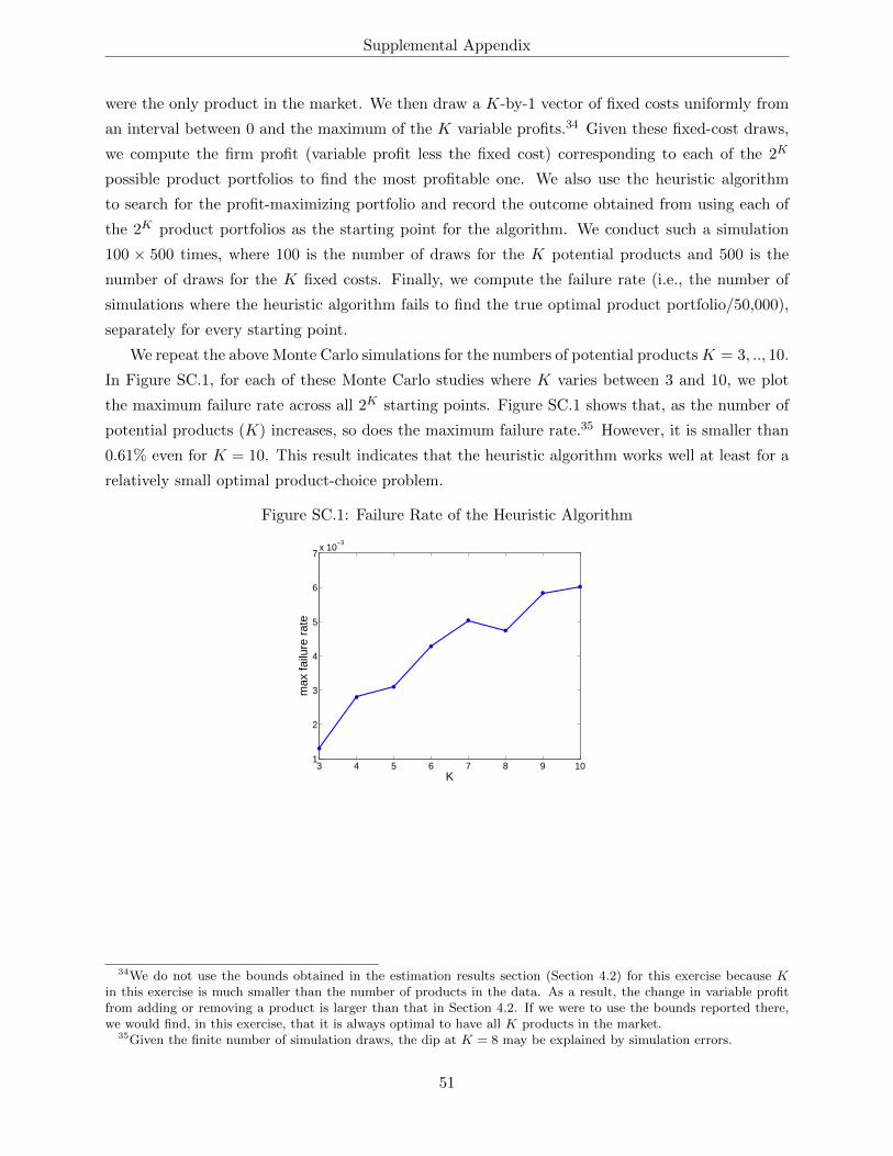
Supplemental Appendix

were the only product in the market. We then draw a K-by-1 vector of fixed costs uniformly from

an interval between 0 and the maximum of the K variable profits.34 Given these fixed-cost draws,

we compute the firm profit (variable profit less the fixed cost) corresponding to each of the 2K

possible product portfolios to find the most profitable one. We also use the heuristic algorithm

to search for the profit-maximizing portfolio and record the outcome obtained from using each of

the 2K product portfolios as the starting point for the algorithm. We conduct such a simulation

100 × 500 times, where 100 is the number of draws for the K potential products and 500 is the

number of draws for the K fixed costs. Finally, we compute the failure rate (i.e., the number of

simulations where the heuristic algorithm fails to find the true optimal product portfolio/50,000),

separately for every starting point.

We repeat the above Monte Carlo simulations for the numbers of potential productsK = 3, .., 10.

In Figure SC.1, for each of these Monte Carlo studies where K varies between 3 and 10, we plot

the maximum failure rate across all 2K starting points. Figure SC.1 shows that, as the number of

potential products (K) increases, so does the maximum failure rate.35 However, it is smaller than

0.61% even for K = 10. This result indicates that the heuristic algorithm works well at least for a

relatively small optimal product-choice problem.

Figure SC.1: Failure Rate of the Heuristic Algorithm

3 4 5 6 7 8 9 101

2

3

4

5

6

7x 10

−3

K

max

failu

re r

ate

34We do not use the bounds obtained in the estimation results section (Section 4.2) for this exercise because Kin this exercise is much smaller than the number of products in the data. As a result, the change in variable profitfrom adding or removing a product is larger than that in Section 4.2. If we were to use the bounds reported there,we would find, in this exercise, that it is always optimal to have all K products in the market.

35Given the finite number of simulation draws, the dip at K = 8 may be explained by simulation errors.

51