Competing for Labor through Contracts: Selection,...
52
Competing for Labor through Contracts: Selection, Matching, Firm Organization and Investments * Orie Shelef, Stanford University Amy Nguyen-Chyung, University of Michigan November 11, 2015 Data is subject to disclosure restrictions. Not for distribution. Abstract Does firm competition for workers lead the best workers to the most productive firms? In a model of of imperfect compeittion for workers through incentive con- tracts, we highlight that while higher-powered incentives attract better workers, higher- powered incentives can reduce incentives for firm investment in productive resources. Driven by this mechanism, firms may endogenously differentiate and sort higher-ability workers into firms with fewer productive resources. Bringing this idea to novel matched employer-employee panel with more than 10,000 firms in residential real estate broker- age where we observe both worker-specific output and incentive contracts, we first de- compose productivity into worker productivity and firm productivity. We find, across all firms and workers, that the best workers do not work at the most productive firms despite complementarity between firm and worker types: firms that are 15% more productive have workers that are 5% less productive. However, within firm that offer the same contracts, better workers do work at more productive firms. We confirm additional predictions of the model on the equilibrium decisions of firms and of work- ers. Consistent with our modelling assumptions, worker heterogeneity and preferences limit the effect of incentives on worker sorting. Counterfactuals show that contrac- tual competition meaningful reduces aggregate productivity by driving better workers to less productive firms. Our work links managerial decisions on incentive contracts and firm investments with labor market competition to explain persistent productivity differences across firms. Keywords: personnel economics, incentive contracts, selection, assortative matching, matched employer–employee data, worker productivity, organizational economics, endogenous firm heterogeneity. * Shelef: Stanford Institute for Economic Policy Research, Stanford University ([email protected]). Nguyen-Chyung: Ross School of Business, University of Michigan ([email protected]). We are grateful to seminar and conference participants at Berkeley, Stanford, the University of Michigan, SOLE, SiOE, NBER SI, and AOM for valuable comments. We thank Sandicor, Inc. and the California Bureau of Real Estate for data access. All errors are our own.
Transcript of Competing for Labor through Contracts: Selection,...

Competing for Labor through Contracts: Selection,
Matching, Firm Organization and Investments∗
Orie Shelef, Stanford University
Amy Nguyen-Chyung, University of Michigan
November 11, 2015
Data is subject to disclosure restrictions. Not for distribution.
Abstract
Does firm competition for workers lead the best workers to the most productivefirms? In a model of of imperfect compeittion for workers through incentive con-tracts, we highlight that while higher-powered incentives attract better workers, higher-powered incentives can reduce incentives for firm investment in productive resources.Driven by this mechanism, firms may endogenously differentiate and sort higher-abilityworkers into firms with fewer productive resources. Bringing this idea to novel matchedemployer-employee panel with more than 10,000 firms in residential real estate broker-age where we observe both worker-specific output and incentive contracts, we first de-compose productivity into worker productivity and firm productivity. We find, acrossall firms and workers, that the best workers do not work at the most productive firmsdespite complementarity between firm and worker types: firms that are 15% moreproductive have workers that are 5% less productive. However, within firm that offerthe same contracts, better workers do work at more productive firms. We confirmadditional predictions of the model on the equilibrium decisions of firms and of work-ers. Consistent with our modelling assumptions, worker heterogeneity and preferenceslimit the effect of incentives on worker sorting. Counterfactuals show that contrac-tual competition meaningful reduces aggregate productivity by driving better workersto less productive firms. Our work links managerial decisions on incentive contractsand firm investments with labor market competition to explain persistent productivitydifferences across firms.
Keywords: personnel economics, incentive contracts, selection, assortative matching, matchedemployer–employee data, worker productivity, organizational economics, endogenous firmheterogeneity.
∗Shelef: Stanford Institute for Economic Policy Research, Stanford University ([email protected]).Nguyen-Chyung: Ross School of Business, University of Michigan ([email protected]). We are gratefulto seminar and conference participants at Berkeley, Stanford, the University of Michigan, SOLE, SiOE,NBER SI, and AOM for valuable comments. We thank Sandicor, Inc. and the California Bureau of RealEstate for data access. All errors are our own.

1 Introduction
Do the best workers work at the most productive firms? Following Becker (1973), matching
arguments suggest they do when labor ability and capital are complements. This positive
assortative matching has important implications for economy-wide productivity. The sorting
literature (since at least Lazear, 1986) suggests that, when firms offer incentive contracts,
the highest-ability workers will choose the highest-powered contracts. In our empirical work,
set in the residential real estate brokerage industry, we find that the best workers do not
work at the most productive firms – on the contrary, we find that firms that are 15% more
productive1 have workers who are 5% less productive. We argue that this result is driven by
the different decisions firms make regarding which contracts to offer and which investments
in firm productivity to make. Like Lazear (2000) and Bloom and Van Reenen (2007, 2010)
our research examines how different firm policies and managerial decisions, including human
capital decisions, lead to productivity variation in firms. We provide theoretical results on
whether and when the most productive firms indeed offer the highest-powered incentives
and attract the most productive workers, and show that our empirical setting matches the
additional predictions of our model.
In this paper, we make three main theoretical and empirical contributions. First, we
develop a model of firms competing for workers through contracts in order to explore the
intuition that high-powered incentives may reduce the incentives for firms to invest in pro-
ductivity. Second, using worker switching to decompose observed productivity into worker
and firm components we provide important evidence that there is negative worker-firm assor-
tative matching in terms of productivity. Third, we show that a number of assumptions and
empirical predictions of our model hold in this setting, and we argue that incentive contracts
are an important driver of negative assortative matching in the real estate industry. More-
over, this trade-off is important at the firm level. Firms that choose to attract higher-ability
workers retain less of the returns to increases in worker productivity, and thus, controlling
for their better workers, are less productive. Our results provide strong evidence that the
competition captured in the model is reflected in economically important magnitudes in the
real world, with important implications for business and public policy.
Following Oyer & Schaefer (2011), we build on theselection effects of high-powered in-
centives, which underlies the notion that incentive contracts increase productivity because
incentives attract higher ability workers. The countervailing force we introduce is that higher
powered incentives reduce a firm’s residual claim on productivity, and thus the incentive for
1Firm productivity, discussed later, is used to describe firm labor productivity, or the value-added toworker productivity.
1

the firm to invest in productive resources. We show that this countervailing force can, in
a competitive equilibria, overcome the selection effect and lead the best workers to high
powered contracts offered by low productivity firms.2
Our theoretical contribution on how incentive structure and firm competition for talent
interact to influence worker sorting and behavior is most closely related to the recent theo-
retical work of Benabou and Tirole (Forthcoming) and older work by Matutes et al. (1994).
However, a key distinction is that we allow firms not only to select workers endogenously, but
also to invest in the productivity of the firm. The idea that productivity may be one dimen-
sion on which firms compete for workers is raised in Gibbons (2005). The trade-off in our
model is similar to that developed in the double-sided moral hazard literature (e.g., Bhat-
tacharyya and Lafontaine 1995) on share-cropping, franchising and other settings, where the
trade-off is due to effort by each of the contracting parties. A similar tension is also present
in the property rights theory of the firm (Grossman and Hart 1986, Hart and Moore 1990),
for instance, in the trade-off between providing investment incentives to the upstream or
the downstream firm. In double-sided moral hazard, the trade-off depends directly on the
returns to effort. In the property rights literature, the trade-off depends additionally on
the outside market’s valuation of the investments. In this work, we focus on the adverse
selection and screening rather than on the moral hazard choices of one party, and we allow
for different degrees of market power on the part of firms.3
A second appealing feature of our model is that ex-ante identical firms endogenously
differentiate both in their organizational form (contract type) and in their complementary
decisions (investments into productive resources.). Thus, we have persistent productivity
differences and persistent organizational heterogeneity identifiable through one mechanism.
In order to apply our theory empirically, we require data with several features. First, we
must observe workers at different firms in the desired setting. That is, we require a panel
dataset of workers across firms, with workers who can and do switch firms. Second, firms
must compete on the basis of incentive contracts to attract workers, and these incentive con-
tracts must differ observably across firms. Third, worker output must be directly observable
or imputable from contracts and wages and comparable across workers and firms.
We choose as our empirical setting the real estate industry because it provides these
features and is also important to the economy. We use data from a large metropolitan re-
2A number of search models (e.g., Shimer and Smith, 2000; Eeckhout and Kircher 2011; Hagedorn andManovski 2014), suggest that despite complementary production functions empirical measures of assortativematching in wages may be negative because of a weak connection between negotatied wages and productivity.Our model allows for negative assortative matching that reflects negative assortative matching measured inproductivity.
3Indeed, one can think of the model we develop below as having workers who vary in productive typeand in how firm-specific their ability is.
2
gion’s residential real estate brokerage industry covering approximately half a trillion dollars
in housing transactions and more than 10,000 firms. We construct a matched employee-
employer dataset leveraging transparency in incentive contracts, complete productivity data
on the entire population of firms in the region and their educated professional workforce,
and accessible information on firm offerings and agent backgrounds . The data also include
substantial worker mobility (over 12,000 workers are with more than one firm across the
study period) and a long span of data (16 complete years) that covers many full careers in
the industry. The dataset combines detailed industry transaction-level data aggregated to
the worker and firm level, government licensing data and a proprietary survey. While such
detailed data may rarely be available in other settings, analogous high and low-powered in-
centive structures and large numbers of heterogeneous firms make this setting generalizable
across many human capital-intensive service industries.4
First, using data on worker productivity across firms, we estimate assortative matching
in productivity terms between worker and firms. This work builds on a large literature fol-
lowing Abowd Kramarz and Margolis (1999) – “AKM” – which decomposes worker wages
into worker and firm effects by asking the question: do high wage workers work at high
wage firms? Recognizing the strong assumptions necessary to interpret high wages as high
productivity, recent work in this literature has focused on the inequality implications of wage
decomposition (Card et al. 2013, Card et al. 2014, Card et al. Forthcoming). In contrast,
our setting allows us to directly observe output and to examine the productivity implications
of matching without those strong assumptions. Like AKM, we use worker mobility between
firms to identify firm and worker effects. We find negative assortative matching between
workers and firms in productivity terms and confirm our findings using a number of alterna-
tive measures that do not depend on this decomposition. Finally, considering the possibility
that firm resources substitute for ability, we use the AKM-style decomposition to examine
the production technology and show that firm resources are complements to worker ability.
Our mechanism drives negative assortative matching between workers and firms by sort-
ing workers across contract types, but generates positive matching of workers across firms
that offer similar contracts. We demonstrate positive matching with-in contract type, and
4There are a number of industries with similar incentive structures and potential selection effects: con-sulting and freelance professionals, law firms, and salons, for instance. Pay-for-performance schemes areincreasingly observed in many sectors – from taxi cab drivers and salespersons to teachers and physicians.Within such sectors, one can also differentiate the sensitivity of such schemes – e.g., taxi drivers in manycities can purchase a medallion or rent a taxi with an upfront payment after which they keep all of theirfares. On the other hand, others may be more attracted to schemes where one pays nothing upfront butkeeps a portion of each fare and shares the remaining portion with the owner or other residual claimant.What attracts workers to sort into these different schemes is of interest, along with what firms offer to inducethe sorting.
3
show that firms with higher powered incentives have better workers and fewer resources.
Together, these findings provide strong evidence that contracts, rather than firms’ choice of
technology or researchers’ choice of measurement, lead to the negative matching of workers
and firms.
In addition to the matching results discussed above and their accompanying sorting
implications, we give empirical microfoundations on the choices of workers and characteristics
of firms. To our knowledge, we are the first to use an employer-employee panel to examine
worker sorting, high-powered incentives, and firm investments across a large population
of firms in an industry.5 Incentive contracts have incomplete sorting effects, consistent
with worker heterogeneity: high-ability workers are disproportionately at the firms with
high-powered incentives, but such firms do not attract an overwhelming majority of high-
ability workers. Workers display rational heterogeneity in risk attitudes, uncertainty about
their own ability, and physical location preferences, as well as unobserved heterogeneity in
preferences for firms. Workers also make trade-offs between their preferences for productivity
investments of firms, such as training and technology, and the immediate compensation
benefits of higher-powered incentives.
We show that firm offerings of productive resources and incentive structures match those
predicted by the model. Firms appear to trade off incentives and productivity-improving
resources as high-powered incentive firms offer lower levels of resources. Moreover, consistent
with endogenous heterogeneity of organizational form, we show that patterns of entry into the
industry by firms offering different levels of incentives match the trends in the population
of workers: high-powered incentive firms follow entry by high-ability workers, while low-
incentive power firms follow entry by lower-ability workers.
Our theoretical work provides a novel mechanism – contractual labor market competition
– which can reduce the extent of assortative outcomes of worker-firm matching. This mecha-
nism is driven by competitive forces and not by wage-productivity disconnects or underlying
production technology. Unlike many models of firms offering incentive contracts that either
examine one firm or hold other firms fixed, our model brings competition between firms into
focus and allows for endogenous heterogeneity of organizational form.
Our empirical findings add to existing knowledge about worker-firm matching6 by find-
ing negative assortative matching in productivity and showing through counterfactuals, that
this result comes at a meaningful aggregate productivity cost. Our empirical estimates of
5Cross sectional or single firm studies include Lazear 2000; Lo et al, 2011; and Bandiera et al. 2015.6Seminal theoretical contributions were made by Becker (1973), and there is a long, and still thriving
theoretical and empirical literature following Abowd and Kramarz (1999) and Abowd et al. (1999), withrecent additions including Mendes et al. (2010), Sorensen and Vejlin (2013), Card et al. 2013, Card et al.2015 and Card et al. 2015.
4

matching are with-in the range of published estimates that rely on various national wage
datasets. While exisiting estimates are low compared with what some established matching
models would have expected, the existing literature is affected by a number of empirical
measurement concerns and theoretical questions about the mapping of wages to productiv-
ity, and has not arrived at strong conclusions about productivity. Empirically, we directly
observe productivity, so we do not depend on a particular mapping between productivity
and wages. Utilizing this we can both estimate matching and examine the complementarity
of the production function. Additionally, we implement several different empirical methods
to address potential estimation bias and identification concerns.7 Our results speak to the
plausibility of small, even negative, assortative matching between workers and firms even
when directly measured and despite complementary production technology.
2 Mechanism
2.1 Intuition of Trade-off
Our model focuses on the role of competition between firms for labor in the trade-off between
attracting higher ability workers and paying those workers larger shares of the return to cap-
ital. Higher powered incentives do both. Because of complementarity between capital and
worker ability, when firms simultaneously make other decisions, such as investing in produc-
tive capital, those investments are increasing in worker quality and decreasing in the workers’
share of output. As we show below, which effect dominates depends on the heterogeneity of
workers in a dimension other than ability and, thus, on firms’ monopsony power. If workers
are relatively homogeneous, the worker ability selection effect dominates and incentive power
and firm investments rise together. However, if workers are more heterogeneous, the residual
claim effect dominates and firms with high-powered incentives invest less.
We make two straight forward departures from Becker style matching. First, we will
assume that workers face frictions embodied in preferences for firms. This leaves firms
with some monopsony power with respect to labor, because workers face varying costs of
switching firms. Second, we assume that firms set wage policies - that is, they choose one
wage function for all workers at the firm, rather than individually negotating wages with
each worker. When combined with monopsony power, firms face intensive/extensive trade-
offs. Changing incentive contracts to attract marginal workers has extensive margin benefits
7We note that, the wage policies in our model and the empirical setting violate the standard assumptionsnecessary to interpret high wages as high productivity. Using compensation structures and observed outputperformance, we impute wages of workers and estimate positive matching between workers and firms withrespect to wages.
5
by attracting workers, it can reduce the rents captured by the firm from its non-marginal
workforce - and intensive margin cost. As in classic models, firms with more productive
resources will generate more surplus attracting more and better workers. However, these
firms potentially face larger intensive margin costs because they generate more rents from
non-marginal workers. What we show below is that when firms compete through contracts
the trade-off between these effects depends on the magnitude of workers’ sorting responses
to incentives.
2.2 Two Firm Framework
In this subsection, we capture this trade-off in a model with two firms.
We consider workers who vary in two uncorrelated parameters: ability a and spatial
location s. The ability heterogeneity of workers generates the potential for quality sorting
and self-selection. For simplicity, we assume that workers are uniformly distributed on the
unit square in ability a and location s and that the two firms are located at the ends of the
square in location space. Location may include physical location, but can also include other
tastes for firm-specific non-produtivity related, amenities. Location captures the worker’s
preference for particular firms separately from compensation. Because firms are equally dis-
tributed in location space, each has equivalent monopsony power over an identical population
of workers. Moreover, ex-ante, firms are identical and face identical populations of workers.
The transport cost parameter, t, captures the degree of competition between firms and
workers’ non-pecuniary valuation of firm characteristics.8 That is, transport costs reflect
workers’ heterogeneity. If s is a worker’s location, then st is how much compensation that
worker requires to work at a firm at location 0. Similarly, the worker requires (1 − s)t to
work at a firm at location 1.
In the first stage, firms choose the type of contract to offer (high- or low-powered), the
parameters of the contract, and how much to invest into capital-like resources r ≥ 1. Later,
we will endogenize the choice of contract type, but for now assume that one firm offers a
high-powered contract and the other a low-powered contract.9 We will refer to these as firm
H and firm L. In the high-powered contracts, workers are paid all of their performance, but
pay a fixed fee f to the firm. In the low-powered contracts, workers pay no fixed fee and
8As is standard, but unlike Benabou and Tirole (Forthcoming), we exclude transport costs from a worker’soutside option.
9While the firm’s contract choice is influenced by the competitive pressures in the simple model, theincentives to endogenously differentiate can arise from other sources. We consider endogenous differentiationlater.
6

are paid half their performance.1011 We scale the utility of the outside option to 0.12 Firms
face a cost of resources c(r) which satisfies the usual INADA convexity conditions from 1.
Capital is any kind of resource that improves the productivity of workers. Our specification
implies capital is a public good with-in the firm. It is non-rival and non-excludable. Our
results are robust to rival specifications, such as a per-worker cost of resources.
Definition. Technology assumption: Output is log-supermodular, that is, the output of
worker of ability a at firm with resources r is ar.
Following the technology assumption, workers’ output is then the product of their ability
and the investments of the firm where the worker chooses to work. An important implication
of the assumption of complementarity between ability and resources is that aggregate output
is maximized when worker ability and firm resources are correlated.
In the second stage, workers observe contracts and investments and choose firms, receiving
utility equal to their compensation less the transport cost times the distance between their
location and the firm they choose. Thus, the utility of a worker of ability a, and location
location s, selecting firm H and L, where the firms choose investment levels rH and rL
respectively, is:
uas(H) = arH − t× s− f
uas(L) =1
2arL − t(1− s)
Workers choose the firm or outside option that maximizes their utility.
Before even considering the firm decisions, conditional on choices of incentive power and
firm resources, several predictions about the choices of workers given the realized choices of
firms follow in Lemma 1.
Lemma 1. (1) Workers of higher ability are more likely to choose firms that offer high-
powered contracts, all else equal.
(2) Workers will prefer firms that offer more performance-improving investments, all else
equal.
(3)Workers of higher ability will, more so than lower ability workers, prefer firms that
offer more performance-improving investments, all else equal.
(4)Workers will prefer firms that are closer to them in location space.
10These two contracts match those offered in our empirical setting. Future models endogenize thesecontracts as responses to the outside option of self-employment by workers and a mass of very low (ornegative) ability workers.
11The model abstracts away from worker moral hazard consistent with our empirical findings, but theresults are robust to including it.
12Future models will endogenize self-employment by workers, effectively allowing the outside option to beincreasing in a and independent of s.
7
Proof omitted. These follow directly.
Lemma 1.1 is the usual sorting result that contracts would generate if firms’ choices
of contracts were independent of firms’ investment decisions. Lemmas 1.2 and 1.3 directly
generate positive assortative matching within firms that offer the same contract, provided
there is heterogeneity in firm performance improvement within a contract type. Lemma
1.4 also results from worker preferences; however, workers’ preferences for different firm
amenities are only observable to a limited extent. We investigate physical distance, though
physical location may be only a small component of the relevant firm characteristics.
To consider the choices of firms, we first define the set of workers that choose each firm.
Let SH(a, rH , f, rL) be the location of the worker who is indifferent between the High firm
and the next best choice, and SL(a, rH , f, rL) be the worker who is indifferent between the
Low firm and the next best choice.13 Thus, the profit function of each firm is:
πH = w ∗ˆ 1
0
sH(a, rH , f, rL)da− c(rH)
πL =
ˆ 1
0
1
2arLÖ(1− sL(a, rH , f, rL))da− c(rL)
The profit functions clarify how the incentives of the firms differ. The high-powered firm
values investments only to the extent that investments attract more workers (regardless of
type) and investments allow an increase in w. The lower-powered firm, in contrast, values
more workers, higher-ability workers, and increases in worker performance generated by
resources.
Proposition 1. (1) At transport costs less than Tr, the high-powered firm has better av-
erage worker ability, more resources, and higher profits than the low-powered firm. (2) At
transport costs between Tr and Tπ, the high-powered firm has better average worker ability,
fewer resources, and higher profits than the low-powered firm. (3) At transport costs above
Tπ, the high-powered firm has fewer resources, lower profits, and, if costs of investments are
sufficiently convex that 2rH > rL, better average worker ability than the low-powered firm.
Proof: See appendix.
The intuition for Proposition 1 follows from two countervailing forces. First, investments
are complements to worker ability, so better workers increase returns to investments. How-
ever, holding workers fixed, offering higher-powered incentives reduces the incentive of the
13Because there may not be an indifferent worker for a particular a, this is defined appropriately as 0 or1 in these cases. In particular, if w > 0, then there are workers at some ability level such that none aremarginal with respect to SH . And, if t is low enough, there are high enough abilities such that no workerswith those ability are marginal with respect to SL.
8

firm to invest because workers are the residual claimants. If labor markets are fluid and
transport costs are low, then the sorting induced by the high-powered incentives outweighs
the reduced incentives. If labor markets are less fluid, the same high-powered incentives
induce less sorting, so the incentive effect takes over.
By analogy, consider the dual problem where firms sell brokerage services to the workers.
This analogy makes market power driven extensive/intensive margin trade-offs standard.
The analog to variation in incentive contracts is variation in price descrimination. A firm
offering high-powered incentives is effectively selling those services at a constant price. A firm
offering low-powered incentives is effectively price-discriminating by charging higher prices to
workers with higher valuations. Investments are now akin to the quality of brokerage services.
Models of a monopolist investing in quality (see, e.g. Tirole 1988) show that, without price
discrimination, the monopolist can extract the return to quality for the marginal consumer
from all consumers who purchase. However, the higher valuation consumers, who value
quality more than do the marginal consumers, keep all their extra benefit. Thus, a flat-price
monopolist invests in quality only to the extent that it improves welfare of the marginal
consumer. A perfectly price-discriminating monopolist, however, extracts all the increases
in welfare from all consumers, so it invests in the first-best quality. Moreover, even if a
price-discriminating monopolist imperfectly price-discriminates, the rents she captures are a
function of the average valuation of consumers. Effectively, this means that the high-powered
commission firm responds fully to the increase in productivity that its investments bring to
its marginal worker. The low-powered commission firm responds partially to the average of
the increases in productivity that its investments bring to all its workers. Which of these
two monopolists invests more depends on a marginal versus average comparison. If part
of the average return to investments exceeds all of the marginal return to investments, the
low-powered firm invests more.
The monopolist analogy removes competition between firms and sorting of workers. The
effects of this competition are important. As transportation costs approach zero, workers
sort perfectly. The marginal high-powered worker at firm H is more productive than all
workers at firm L (and thus any average of the firm L’s workers), so firm H invests more.
With higher transport costs, some high-ability workers choose the low-powered firm, and
the average of a distribution of workers with a lower mean ability can exceed the marginal
worker in a higher-ability distribution of workers. The nature of competition, captured in
the transport costs and worker heterogeneity, drives whether resources and incentives are
strategic compliments or substitutes.
The two-firm model shows the key empirically relevant insight – why firms that offer
lower-powered contracts might invest more in capital. Importantly, this dynamic is contin-
9

gent on the effectiveness of high-powered incentives in attracting high-ability workers. More
heterogeneous workers, reflective of a less fluid labor market, push the labor market toward
a situation where negative matching between workers and firms is driven by contracts. In
the appendix, we generalize to the case of many firms, considering endogenous contract type
choice and free entry of firms.
2.3 Testable Hypotheses
Taken together, our argument has important implications for how compensation and re-
sources impact sorting induced by pay-for-performance. The same logic that makes high
pay-for-performance attractive for high-ability workers undermines investments in resources
by the firm. The models generate a number of empirically relevant hypotheses. We collect
them here. First, Hypothesis 1 follows by definition from the negative assortative matching
equilibrium. Hypothesis 2 and Hypothesis 3 are effectively consequences (and tests) of the
technological assumption and are predictions independent of negative assortative matching.
In the model as written, however, there is no variation in productivity within each contract
type, so empirical testing would be difficult. However, with other sources of heterogeneity
within a contract type, Hypothesis 2 is testable. Hypothesis 3 follows directly from the tech-
nology assumption, while Hypothesis 2 follows from Lemma 1.3, in that firm productivity is
differentially valued by high-ability workers, so that they sort into high-productivity firms
if there are no other differences between firms. Hypotheses 2 and 3 are what drive a broad
class of models, including search models, to expect positive assortative matching.
Hypothesis 1. Productivity of workers and firms will be negatively correlated across all
contract types.
Hypothesis 2. Productivity of workers and firms will be positively correlated within firms
that offer the same contract.
Hypothesis 3. The production technology displays supermodularity – higher ability workers
gain at least as much in productivity from increases in firm productivity as lower ability
workers.
We then have Hypothesis 4, which describes the characteristics of firms. The first 4
characteristics follow directly from negative assortative matching as seen in the two firm
model. In negative assortative matching equilibria of the two firm model high commission
firms have lower per worker and aggregate profits. With free entry & endogenous firm choices,
the even division of firms is not sustainable. Firms will shift twoards low-commission until
profits equalize, yield characteristics (5) and (6).
10

Hypothesis 4. In a negative assortative matching equilibrium, firms that offer high-powered
contracts, compared to low-powered firms, will:
(1) Have workers with more productive ability,
(2) Offer fewer productive resources,
(3) Draw workers from greater distances,
(4) Attract a disproportionate share of high ability-workers,
(5) Have more workers, and
(6) Be relatively rare.
Following directly from Lemma 1, we have Hypothesis 5, which describes the workers’
preferences among firms. Hypotheses 5.1-5.3 follow directly from the Lemma 1 characteristics
of firms. Hypothesis 5.4 follows from a combination of Lemma 1.4 that says workers value lo-
cation space and the previous prediction thathigh-powered firms are rarer. With unobserved
heterogeneity in firms, workers will likely find the most highly preferred low-powered firm
to be a better match in location space than the most highly preferred high-powered firm,
even when contract and investment choices by firms do not depend on firms’ unobserved
heterogeneity.
Hypothesis 5. In a negative assortative match equilibrium, workers will, all else equal,
prefer firms that
(1) Offer a contract more suited to their ability,
(2) Have more resources,
(3) Are physically closer, and
(4) In the presence of unobserved firm characteristics, will over-value the low-powered
incentive firms.
Hypothesis 6 focuses directly on the implication that, if workers are distributed in location
space, we will observe heterogeneity in sorting patterns. Hypothesis 6.2, however, goes
directly to the key heterogeneity requirement for negative assortative matching to be in
equilibrium: that even firms with low-powered contracts will attract sufficient high-ability
workers. Because workers select firms for many characteristics, incentive power has only a
moderate effect in generating sorting, and low-powered firms can capitalize on the possibility
that they will attract a high-productivity worker.
Hypothesis 6. In a negative assortative matching equilibrium, worker-firm sorting patterns
will reflect worker heterogeneity:
(1) Workers will show heterogeneity in preferences for firms.
11

(2) Low-powered firms still capture an important share of workers of very high ability.
Unmodeled heterogeneity in risk attitudes, worker uncertainty about own ability, and worker-
career dynamics magnify the matching.
Finally, because we observe exogenous changes in the performance of agents, we consider
what happens as the distribution of workers’ abilities change. Following from the intuition
of endogenous entry and contract choice, firms will follow their respective population of
workers.
Hypothesis 7. An increase in the number of high-ability workers leads to more firm entry
and an increase in the share of high-powered incentive firms. An increase in the number
of low-ability workers leads to more firm entry and a decrease in the share of high-powered
incentive firms. If the distribution of worker ability changes, high-powered firms enter in
response.
3 Institutional Context and Data
We examine these issues in a large metropolitan region’s residential real estate brokerage
industry. Heterogeneous and mostly transparent incentive contracts, productivity and back-
ground data on the full area population of firms and their educated professional workforce
allow us to construct an ideal matched employer-employee dataset. Other desirable features
of the data include substantial worker and firm heterogeneity, substantial worker mobility,
free entry and exit of individuals and firms and a long span of data (16 complete years ).
The housing market, valued at $27.5 trillion at the end of 2014, is a critical component of the
US economy, and over half a trillion of that dollar value is situated in the study area. The
residential real estate brokerage industry is also approximately 0.8% of GDP and employ-
ment. The number of licensed agents in California peaked in 2007 at about 550,000 agents,
or one out of every 66 people (DRE and US Census). 14
Agents join a firm, whether it be a small independent firm with a single broker-owner, a
locally-based regional independent with hundreds of agents, a franchised office of a national
chain, or one of their own creation.15 They select firms based on many reasons, including
incentive structure and productive resources such as strong brand recognition and training,
and non-pecuniary reasons such as coworkers and proximity to their homes. Interview and
survey data point to resources such as training and brand and more appealing incentive
structures as the dominant reasons that agents switched firms.
14Not all agents with unexpired licenses are active in residential real estate brokerage.15We do not focus on entrepreneurial choice in this paper; it is the main subject of Nguyen-Chyung (2013).
12

Firms set the incentive structure, make investment decisions regarding productive re-
sources and employ workers. Among the productive resources provided by firms include:
office space and equipment, advertising, networks, training, mentoring, leads and referrals,
IT support and back office services. Firms attract, support, supervise, motivate and retain
agents. These decisions and tasks can be time-consuming and require significant investment.
To construct our data, we first leverage a dataset derived from the confidential set of
Multiple Listing Service (MLS) data in San Diego County, CA.16 The data lists every listing
and sale (if any) of virtually all agent-mediated residential real estate transactions handled
though the full metropolitan area MLS. Crucially, each transaction listing identifies the buy-
ing and selling agents and associated firms as well as corresponding sale price. Effectively,
the MLS is a list of the production of the residential real estate industry attributed not just
to firms, but also to the individual workers at those firms. Following the approach taken in
Nguyen-Chyung (2013), for each real estate agent, we record a career path through firms and
combine the career histories with state licensing data and a survey of a random sample of
agents to obtain additional agent information, such as risk attitudes and rationale for switch-
ing firms.17 Any time an agent lists a client’s property, or helps a client purchase property, he
or she must report the transaction details into the MLS. Each productive act thus provides
the productivity and firm affiliation of the worker. We now further aggregate the data to
the firm level and additionally gather firm-level information systematically for all the major
real estate firm brands through primary and secondary sources (including interviews and
real estate franchise reports).18 The resulting dataset consists of a new employee-employer
linked panel with worker-specific productivity, for the population of approximately 40,000
agents and 10,000 firms that were active in the county for any part of the period between
1995 and 2011, inclusive. The data appendix describes the construction of the dataset.
Our main unit of analysis at the firm level is the firm-office, because many real estate
offices are operated independently even in national real estate chains. Additionally, firm-
offices are assigned into groups of national, regional and local chains (franchise or otherwise).
For these chains, we have gathered information on the standard contracting offer the firms
make to potential agents. For national franchises, we gather the upfront franchise fee or
expected investment by new franchisees. For most of our individual analysis, we aggregate
the data to calendar year-worker, assigning the productivity of the worker to the first firm
16San Diego County, with a population of over 3 million people, is bounded geographically on all four sidesby natural or national borders, and thus has minimal unobserved agent activity in other regions.
17We map agents in the MLS data to the license data using license number data when available, names,date range of activity, and geographic location.
18The data linking follows that of Nguyen-Chyung (2013), except that, instead of stopping at the individuallevel, we further aggregate individuals and production at the firm level.
13

observed in the year. The data allow us to observe entry of both firms and individuals.
When individuals and firms stop having productive events, we note exits.
We measure production as the industry does, using commissions generated by each trans-
action. For a majority of the transactions, the data report the commission rate offered to the
buyer’s agent. Relying on the strong symmetry norm, we assign an equal commission rate
to the seller’s agent. We use the mean commission rate where none is reported. Results are
very similar if we measure production by dollar value of houses sold. Effectively, all agents
are paid entirely on a contingent basis and earn commissions only on the value of the trans-
actions they complete.19 Firms rationally would like to hire an unlimited number of these
costless workers, except perhaps an occasional “bad worker” (e.g., an unethical person) who
might create some liability for the firm or those with very low motivation who may affect
the morale of the other workers.
Real estate agents who do not own their firms receive a portion of real estate commissions
based on their commission-split with the managing broker or broker-owner for whom they
work. Two splits are particularly common in the industry. “Traditional” or “standard”
firms offer no fixed wage and a split of about 50-50%.20 In many other industries, these
incentives would be very high-powered. However, the next most common compensation
arrangement has agents pay a desk fee – essentially a negative fixed wage - and keep all of
the commission (i.e., 100% commission split). This “high commission” compensation system
is thus of higher sensitivity (as evidenced by the higher slope of the incentive contract) than
other pay-for-performance contracts in the industry.
4 Matching
Our primary mechanism to examine the assortative matching of workers to firms is to decom-
pose productivity into worker and firm components and examine the matching of workers to
firms. We do this by implementing AKM decomposition. AKM decomposition, traditionally
applied to wages, uses workers who switch firms to identify worker and firm effects via OLS.
Thus, we estimate a high-dimensional fixed effects model
log(Revenueijt) = βXit + δi + γj + λt + εijt
19There are a handful of exceptions who may receive some fixed wage component: those who work forhomebuilders, lenders and a very small number of salary-based firms.
20There are small variations in the split, such as payment of the royalty to the national franchise. In thatcase, royalties of about 6% are paid before the broker and agent’s split.
14

where we regress the revenue production of worker i and firm j in year t on time-varying
worker observables X and worker, firm, and year fixed effects. We estimate via OLS. Our
primary parameter of interest is the assortative match parameter, the correlation between δi
and γj, which indicates whether the higher productivity workers are at higher productivity
firms. 21
The interpretation of the worker and firm fixed effects is worthy of discussion. Worker
fixed effects capture the estimated output of the worker at a fixed firm after adjusting for
the year effect and the experience of the worker. It also can be interpreted as worker quality
or accumulated human capital. We do not observe, independent of output, any measures of
effort for any worker. To the extent a worker is part-time or exerts extra effort, she is simply
observed to be less or more productive.22 The firm fixed effects, then, measure the change
in workers’ output at different firms, which can be naturally interpreted as the firm’s valued
added – how much more productive the firm makes the worker. The fixed effect is equally
interpreted as labor productivity of the firm – how much output the firm produces for a unit
of labor. A unit of labor in this definition, however, is not an hour of labor, but rather a
human capital adjusted year of labor. If a firm is able to produce more with a unit of labor,
it has higher labor productivity.23 The total productivity of the firm is the combination of
both fixed effects and time-varying characteristics.
4.1 Mobility Driven Estimation
As is standard in the literature, we can only estimate this on a connected set of workers and
firms. That is, if there is no mobility between two groups of firms, the productivity of the
second group of firms cannot be estimated. Consistent with earlier literature, we restrict
attention to the largest connected set, which contains approximately 158,000 worker-firm-
years. The next largest connected set contains 45. Table 1 provides additional summary
statistics. The largest connected set covers 95% of the revenue generation and 90% of the
worker-firm-years in the data. Two caveats about the sample are worth mentioning. First,
approximately 15% of the entire sample is composed of broker-owners, that is, agents who
employ themselves and potentially others. However, about 52% of the omitted worker-firm-
years are broker-owners. Simply put, the productivity of these primarily sole practitioners
21Our primary measure of output is Revenue. In the appendix we estimate a model with transactions asthe dependent variable. To do so, we extend AKM style decomposition to Poisson count models. Resultsare similar.
22The survey captures whether residential real estate is workers primary activity. Approximately 25% ofworkers report that it is not. These workers are estimated to have worker fixed effects that are 0.13 lower.
23Both our theoretical model and our empirical specifications exclude moral hazard effects. This is aconservative assumption that makes high-commission firms, which presumably induce more effort, havehigher labor productivity.
15

is not decomposed into workers and firms. If workers start their own firm by 1995, remain
there, and have no employees, they are outside the connected set. Consistent with this, the
excluded firms are far fewer – an average of 3 worker-firm-years per firm, compared to 31 for
the included set.
Because the AKM estimation uses movers to identify firm fixed effects, in Table 2 we
present descriptive statistics of movers compared to workers who appear only in a single
firm. Movers are the majority of firm years and revenue and are approximately 36% of
workers. Figure 1 shows the share of worker-firm-years that movers represent, by log revenue
generated. Movers represent the majority of revenue generation and a large share of workers.
For the OLS estimates to be unbiased, we require that:
E[(εijt − εi)(Djit − D
jit)] = 0 ∀j.
where Djit is an indicator for employment at firm j in year t and bars represent averages
over t. That is, we require worker mobility to be uncorrelated with εijt. To understand the
implications of this assumption, we could further decompose εijt into pairwise components:
match effects, firm shocks and worker shocks. εij captures the time-invariant worker-firm
productivity match. That is, if workers and firms have specific productivity match effects,
and if mobility were based on this match, then firm choice would depend on match-specific
values. In the search literature models of dynamic matching, increases in match-specific
productivity are the reason for worker mobility. In those models, however, mobile workers
always increase their productivity. Below, we examine the productivity gains of workers who
leave and workers who join firms. To do this, following Card (forthcoming), we first bin each
firm by the average co-worker log-output into four quartiles. We then characterize each move
as a move from one of the four quartiles to another of the four quartiles. For each type of
mobility event, e.g., moving from a 1st to 3rd quartile firm, we calculate the average output
change. We then plot this by direction – that is, plot 1st to 3rd versus 3rd to 1st. Under
productivity matching, these transitions would always be positive. Under the estimating
assumption, these should be approximately symmetric – 1st to 3rd switchers improve by
about the amount that 3rd to 1st switchers reduce their output. Figure 2 displays the
approximate symmetry of productivity changes when workers move in opposite directions
between firm bins. If workers moved to higher productivity matches, as in typical match
models, these observations would lie in the first quadrant, not the fourth. Our results are
inconsistent with productivity match-specific firm selection. As an additional comparison
we estimate a model with fully saturated worker cross firm fixed effects, and compare the
fit of that model to the model with separate worker and firm fixed effects. The adjusted R-
16

squared of the interacted fixed effects model with 53,937 fixed effects is 0.615 and the worker
and firm fixed effect model with 31,747 fixed effects has an adjusted R-squared of 0.584. As
expected, the interacted model fits better, but increases the R-squared by only 3 percentage
points. Additionally, the coefficients on the time varying fixed effects are economically and
statistically similar.
Firm-specific shocks – the success or failure of particular firms – would appear in εjt.
If workers are more likely to leave failing firms and join successful firms, firm choice would
be correlated with the error term. We look for “Ashenfelter dips” (1978) in the output of
leavers and bumps in recent hires. To do this, we plot each of the 16 move types, the path
of worker performance before and after moving, using the same bins described above and
restricting the data to movers whom we observe for two years before and two years after
transitions.24 Figure 3 displays the trends of productivity for movers from the bottom or
top quartile firms.
Finally, we consider worker-specific time shocks, εit, because workers whose productivity
has had a positive shock might be more likely to move to a particular kind of firm, implying
a systematic pattern in the productivity of workers prior to switching. If, within the same
original type of firm, workers who go to different types of firms exhibit different trends before
moving, such a pattern suggests violations of the OLS assumption. Similarly, the assumption
might be violated if workers from different firms who have moved into similar destination
firms workers displayed different trends after moving.These effects would be visible in Figure
3. Level differences by origin or destination are to be expected, if workers are sorting by
type, but, for most switches, such trends are not statistically distinguishable.
What sources of mobility remain? What mobility reasons are not problematic for OLS
specifications? First, mobility that is driven by δi, that is, by fixed worker characteristics,
does not bias our measurement; examples include matching worker ability to the appropriate
firm contract or movements of workers of different abilities to firms of different productivities.
Second, firm mobility due to different firms being located in different locations in non-
productivity space does not bias our estimates, because workers have preferences for firm
characteristics. Finally, mobility because of predictable career dynamics, such as joining a
high-resource firm prior to becoming a sole proprietor, does not bias our estimates.
4.2 Limited Mobility Bias
There is an additional source of bias that is present in small sample estimates of the assor-
tative match parameter: the correlation between workers that can occur even if the OLS
24Workers may appear more than once if they have more than one move that meets these criteria.
17

parameters are unbiased. This correlation occurs because the assortative match parameter
captures the correlation between parameters, and, in small samples estimation error, may be
correlated. That is, if a worker’s fixed effect is underestimated, that will lead to an upward
bias in the estimate of firm effects at the firms where he worked. Because we observe only
a short panel for each worker, estimation bias is meaningful and likely understates the ex-
tent of positive assortative matching. We address this bias in several ways. First, following
Andrews et al. (2008), as implemented in Gaure (2014, 2015), we can estimate the bias in
a manner akin to shrinkage of random coefficients. The firm and worker fixed effects are
over-dispersed, and their correlation is biased. Andrews et al. (2008), under the assumption
of iid errors, derive the corrections. As Card et al. (Forthcoming) notes, wage data likely
display a number of correlations in the errors, such as serial correlation due to wage rigidity,
which would make these corrections insufficient. Importantly, we observe productivity rather
than wages. In our setting, we see little of the serial correlation that would complicate bias
correction. we estimate the serial correlation of productivity in a model with worker-by-firm
fixed effects. We find that ρ=-0.014, so the Breusch-Godfrey test for serial correlation does
not reject the null of no first-order serial correlation. If we did indeed have negative serial
correlation, the bias correction below would over-correct our estimates.
Our second approach to considering correlated errors is to use 2SLS to correct for mea-
surement error. By instrumenting for δi in a regression of firm fixed effects on worker fixed
effects, we can correct for the correlational error. This method does not correct for the over-
dispersion, so it is difficult to compare magnitudes directly. We instrument for a worker’s
fixed effect by whether he began his California real estate career in San Diego County, as
“natives” are more productive. We measure this by using the location of the agent’s licensing
exam. We rely on our bias-corrected adjustments as our primary measure.
In the appendix, we perform several validation exercises and alternative bias correction
methods. To validate our estimates, we estimate models where we subsample our data, mag-
nifying the short panel/limited mobility bias and the bias correction. If the bias correction
is performing correctly, those estimates should be similar to the bias corrected results on the
full sample. Second , we estimate clustered bias correction as suggested by Gaure (2014). We
also perform several bias alleviation methods that involve further restricting the estimation
sample. As Andrews et al. (2008) point out, while estimation bias is reduced in samples
with more mobility the underlying matching may differ between samples. Using German
aggregate data, they find more assortative matching, after bias correction, in samples with
more movers. Sample restrictions drop firms with few movers - in our setting, potentially
relatively able workers at small firms (such as their own). In the appendix we implement
split-sample estimation where we divide the data in half, and estimate the correlation be-
18

tween worker effects from one sample and firm effects from the other - thus correcting for the
incidental parameter bias, but not the over dispersion of fixed effects. Similarily, we examine
the correlation when we restrict to firms with varying thresholds of movers.
Existing literature has estimated the match parameter in AKM type models, but has
not reported confidence intervals or statistical tests regarding the parameter. Here, we im-
plement two bootstrap methods. First, using the estimated variance of the worker and firm
fixed effects, we draw normally distributed random fixed effects, assign them to the workers
and firms without correlation, and estimate the correlation given the mobility patterns in
our data. Second, we implement the much more computationally intensive method of boot-
strapping our total estimate strategy. The first method makes a distributional assumption,
while the second relies on the bias correction being correct for different bootstrap samples.
4.3 Productivity Decomposition and Assortative Matching
With these results, we turn to the productivity decomposition itself. Figure 4 displays the
firm and worker fixed effects, prior to small sample bias correction. The red solid line plots the
unbias corrected correlation. Plotted in the green dashed line is the the estimated correlation
of worker and firm fixed effects, after bias correction, of -0.04***. This estimate is within
the range of published estimates of worker-firm matching using economy-wide wages. The
economic magnitude of this estimate is meaningful. Firms that increase the productivity
of workers by 15% more have workers who are 5% less able. Consistent with real estate
brokerage being a human capital intensive industry, variation across workers in ability is
much larger than variation across firms in productivity. One standard deviation in worker
ability is an 80% difference in ability, while a standard deviation in firm productivity is a 26%
difference. Firm productivity matters in economically meaningful magnitudes, but workers
are the bulk of the variation.
As an alternative bias correction methodology, we instrument for a worker’s fixed effect
by whether the worker began his California real estate career in San Diego County mea-
sured by having taken the real estate licensing exam in San Diego. Consistent with results
elsewhere, the first stage is strong and predicts that locals are more capable agents. An
important assumption in the exclusion restriction is that workers who began in San Diego
and those who did not gain equally from firms. An analysis of the residuals cannot reject
the null that natives and non-natives gain the same from firms, while the point estimates
suggest that those who began their career in San Diego gain a bit more than firms, leading to
more assortative matching. Table 3 reports the OLS, unbiased corrected estimate of regress-
ing firm fixed effects on worker fixed effects, the first stage, and the instrumental variable
19

estimates. Note that because this method does not adjust for over-dispersion in the fixed
effects estimates, it is not directly comparable to the bias-corrected correlation. However,
our confidence that we are not under-bias-correcting is increased because our results are very
similar to the OLS, both in magnitude and sign.
For our final evidence of the direction of assortative matching, we examine correlation
between the experience of workers and the productivity impact of firms. Because the industry
displays strong returns to experience, and experience is controlled for and measured, we
estimate the correlation between worker experience and firm fixed effects. Note that, since
experience is controlled for in the decomposition, the assortative matching here is not a
measure of the same assortative matching between fixed effects – it should be additive
and is not subject to small sample bias, because we are not comparing joinly estimated
fixed effects. Figure 5 displays the average estimated firm fixed effects by year of worker
experience. Table 4 presents the underlying regressions. Each additional year of workers’
experience lowers the expected productivity of their firm by 0.6%, while it increases worker
performance by 2.3%. Interestingly, this ratio of effects is similar in negative assortativeness
to the negative correlation between fixed effects. Moreover, Figure 5 is consistent with links
between experience and productivity, controlling for firm cross worker fixed effects that show
decreasing improvements in productivity, with small increases in productivity between 10
and 20 years of experience, and almost no improvements there after.
We also estimate an additional decomposition, where we replace log(revenue) with
log(wagej(revenue) + minwagej(revenue)∀j), where wagej(·) is the approximate compen-
sation structure for the firm. Because realized wages may be negative, despite positive wage
generation, we add the minimum to all values. Our estimate of the bias-corrected correlation
between worker and firm fixed effects in wages is 0.01*. This positive correlation is consistent
with workers sorting across contracts into firms that pay them more, although, as we show
below, high-commission firms have fewer productive resources.
4.4 Production Technology
We perform a few additional analyses using the decomposed productivity estimates to high-
light the production technology and role of contracts. First, we repeat our bias-corrected
estimate of assortative matching on restricted samples to measure the assortativeness of
matching among firms that offer similar contracts. To do this, we restrict the analysis to
firms that we observe the contract type, and separately for each contract type, we estimate
the bias-corrected estimate of assortative matching. This provides us a measure of within-
contract sorting. We exclude firms for which we do not have identified contract types, or the
20

contract type for the firm is unique. In Figure 6 we present two: “high-commission” firms
where the contracts offer agents at least 90% of the marginal commission they generate, and
“traditional” commission firms where new agents earn approximately 50% of the marginal
commission they generate. Even prior to bias correction, both show positive assortative
matching. Within high-commission firms, the bias-corrected covariance of worker and firm
fixed effects is 0.078***; within traditional commission firms, it is 0.072***. These capture
the effects matching driven by labor productivity, but not that driven by worker selection
of contracts. These separate the matching effect into those driven by firm resources, but
not by sorting across contract types. It provides evidence that matching is more assorta-
tive and positive within contract types is consitistent both with complementary production
technology and contractually driven negative assortative matching.
Second, we examine the fit of the functional form of our empirical model. Our estimation
assumes a Cobb-Douglas, or an additive in logs, production function, which embeds propor-
tional complementarity between workers and firms. Specifically, we want to ensure that the
complementarity between worker ability and firm productivity embedded in the functional
form of our specification is a good fit to the data. This is relevant both to the appropriate-
ness of the empirical specification we have fit and to the appropriateness of the assumption
of complementarity between workers and firms our theory assumes. We bin the workers and
firms each into 10 bins by estimated fixed effect, and, for each of the 100 combinations, plot
the mean residual in Figure 7. This diagnostic tells us, for example, whether the model fits
poorly, e.g., if there are large mean residuals. We find small mean residuals are small. All
are less than 1.5 percentage points. That is, our log assumption of the functional form of
the production function is within 1.5 percentage points of a non-parametric estimate that
allows separate effects for each combination of decile. This result occurs despite a significant
increase in degrees of freedom. The log functional form uses 20 degrees of freedom (the
mean residual within each row and column is 0), while the non-parametric version would use
100. More over, it also informs us of systematic deviations from the production function we
estimate. Systematic deviations would appear as a pattern in the residuals. For example,
ff firms and workers were less complements than we assume, mean residuals for high decile
workers at high decile firms would be negative and those for low decile workers at low decile
firms would be positive and the graph would flow from dark red in the top left to dark blue
in the bottom right. We do not observe such a pattern of residuals in our data which sug-
gests that our production function fits well. Indeed, regression versions of this optical test,
which regresses residuals on the interaction of types yields small, positive, insignificant, and
tightly estimated coefficients. We can reject that the production technology deviates far from
log-complementarity, and, if anything, ability and resources are even stronger complements.
21
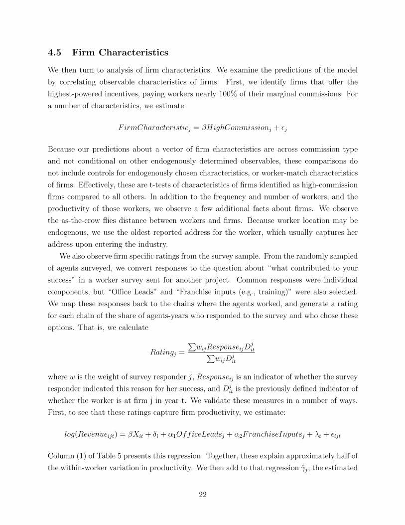
4.5 Firm Characteristics
We then turn to analysis of firm characteristics. We examine the predictions of the model
by correlating observable characteristics of firms. First, we identify firms that offer the
highest-powered incentives, paying workers nearly 100% of their marginal commissions. For
a number of characteristics, we estimate
FirmCharacteristicj = βHighCommissionj + εj
Because our predictions about a vector of firm characteristics are across commission type
and not conditional on other endogenously determined observables, these comparisons do
not include controls for endogenously chosen characteristics, or worker-match characteristics
of firms. Effectively, these are t-tests of characteristics of firms identified as high-commission
firms compared to all others. In addition to the frequency and number of workers, and the
productivity of those workers, we observe a few additional facts about firms. We observe
the as-the-crow flies distance between workers and firms. Because worker location may be
endogenous, we use the oldest reported address for the worker, which usually captures her
address upon entering the industry.
We also observe firm specific ratings from the survey sample. From the randomly sampled
of agents surveyed, we convert responses to the question about “what contributed to your
success” in a worker survey sent for another project. Common responses were individual
components, but “Office Leads” and “Franchise inputs (e.g., training)” were also selected.
We map these responses back to the chains where the agents worked, and generate a rating
for each chain of the share of agents-years who responded to the survey and who chose these
options. That is, we calculate
Ratingj =
∑wijResponseijD
jit∑
wijDjit
where w is the weight of survey responder j, Responseij is an indicator of whether the survey
responder indicated this reason for her success, and Djit is the previously defined indicator of
whether the worker is at firm j in year t. We validate these measures in a number of ways.
First, to see that these ratings capture firm productivity, we estimate:
log(Revenueijt) = βXit + δi + α1OfficeLeadsj + α2FranchiseInputsj + λt + εijt
Column (1) of Table 5 presents this regression. Together, these explain approximately half of
the within-worker variation in productivity. We then add to that regression γj, the estimated
22

firm fixed effect. The addition makes both estimates statistically and economically zero
and explains only about 3% more of the variation. That is, the combined effect of these
two ratings in predicting the productivity impact of a firm is approximately 94% of the
variation captured by firm fixed effects. Finally, to connect these measured firm resources
to investments by firms, in Table 6, we use our estimated investment costs of franchise to
show that firm ratings are correlated with actual investments by entrepreneurs when they
establish firms. Sensibly, we see a correlation between franchisee expenditures and franchise
inputs. However, both firm firm fixed effects and office leads have important subtitutes to
the nationally provided franchise effects, so that firms that do not buy these from a franchise
may procure them in other ways.
We now turn to the results about the structure of firms. Figure 8 plots these as graphs.
High-commission firms represent just under 10% of all firm-years, i.e., of all employment.
Consistent with the model, high-commission firms attract workers an average of 1.5 miles
farther away. These workers are about six months more experienced as well. Consistent
with having lower per agent profit, as is predicted in the negative assortative matching
equilibrium, high-commission firms are larger, with about three times as many workers per
year on average.
We also present evidence that high-commission firms are lower in productivity. Figure 9
shows that our estimated fixed effects are lower for high-commission firms, though noisily,
at least partially because of small-sample bias. Figure 9 also provides evidence that high-
commission firms have lower survey ratings.
In our final analysis of firms, we examine how the different types of firms enter or exit
in the boom and bust in the real estate market. During the boom, we observe entry by
agents such that the distribution of workers changes. In each year, we divide workers into
high-ability and low-ability workers, where the dividing line is $100,000/year in revenue.
Figure 10 plots how the number of firms of each type and the number of workers of each
type evolve. During the period of this data, in this geographic location, the market grew in
size without a dip between 1995 and 2004. 2005 was slightly smaller than 2004, and then
the market declined through 2011. Importantly, market size is a factor related to both prices
and volume. While prices peaked later, volume times prices peaked in 2004. Several facts
are worth noting. First, the peak in high-commission firms is in 2004, as is the peak in
high-ability workers. Low-commission firms and low-ability workers peak in 2006. Second,
exit takes several years. Despite a stark decrease – market size in 2011 was less than half of
2004 – firms persisted for several years after the decline became obvious in 2006 and even
after the subprime market collapse in 2008, perhaps not quite reaching equilibrium by 2011.
23

4.6 Worker Sorting
Finally, we turn to our analysis of worker firm choices and heterogeneity. Effectively, these
are checks of our model’s assumptions that workers value productive resources, contracts,
and non-productive and compensatory aspects of firms. To examine how workers trade off
various firm characteristics, we estimate logit models on whether a worker changes firms this
year with respect to the resources of his current firm (productivity fixed effect, office survey
ratings, physical distance) and worker characteristics. That is, we estimate models of the
form:
Moveijt = αFirmCharacteristicj + βWorkerCharacteristici + λt + εijt
Table 7 presents several specifications predicting whether a worker will change firms, depend-
ing on the observable characteristics of the firm and match. The better (more productive)
the firm, and the better the match (closer in physical space), the less likely the worker is to
depart. One note, beyond that expected in the model, is that workers appear to value firms’
Franchise Input Rating, but do not value office leads beyond the effect through compensa-
tion. This observation is consistent with workers’ investment in human capital by remaining
at high-franchise input firms, because these firms offer training which has both immediate
output effects, captured by firm fixed effects, and potentially persistent effects not captured
in the firm fixed effect.25
For each mover, we predict the difference in expected wage the following year at an
average productivity high-commission firm and at an average traditional commission firm,
using the estimated worker ability, firm productivities, and experience effects. We then
estimate where workers go, conditional on moving.
HighCommissionijt = αPayDifferenceijt + εijt
The model suggests, first, that this coefficient will be large and significant – those who
benefit more from high-commission firms should be more likely to select them. Second, the
model suggests that correlated, unobservable workers’ idiosyncratic preferences will bias this
estimate downward. Table 8 shows that, conditional on switching firms, workers with more
to gain, as estimated by the predicted wage difference between a traditional firm and a high-
commission firm for a worker with the appropriate fixed effect, is an important predictor
of firm choice. However, consistent with the predicted unobservables about the firm, this
25In related preliminary work, we show that high-franchise input firms have persistent effects on workersoutputs, even once those workers leave the firm.
24

coefficient is likely too small. The logit estimate suggests it takes approximately $700,000 in
expected income increase to make half of workers choose high commission firms.
Finally, we provide evidence of worker heterogeneity. First, in aggregate, we non-
parametrically fit the share of workers at high commission firms by worker ability. If het-
erogeneity is important, this share should be increasing with ability, but high-commission
firms will not have a disproportionate share of such workers. Figure 11 graphs the share
of workers at high-commission firms by annual revenue. Approximately 20% of the best
workers are at high commission firms, leaving approximately 80% of the best workers not at
high-commission firms.
We then investigate several specific sources of heterogeneity. While many dimensions of
heterogeniety are likely unobservable except through firm choice, here we present evidence
describing several dimensions of heterogeneity that we do observe. In Figure 12 we plot
workers’ distance to their first firm.
Next, we examine the importance of risk aversion heterogeneity using survey-based mea-
sures of the distribution of risk aversion and non-parametric estimates of uncertainty. We
do this in two steps. One of the survey risk questions asks respondents to select among
lotteries, as is standard in measuring risk aversion. We map these responses back to the
wealth of respondents as measured by their census block group, and estimate a distribu-
tion of the coefficients of risk aversion. Then, to determine the thresholds at which agents
of different risk aversion would prefer high-powered commissions over traditional commis-
sion firms, we present a non-parametrically smoothed change in utility between the two
extreme contracts. Figure 13 plots the survey responses.26 Those who answered 80 or 100
have RRA<1; those who answered 0 or 20 have RRA>4; and the rest lay in between. For
each risk aversion parameter, we convert next year’s revenue into an expected utility differ-
ence, and non-parametrically smooth that with respect to this year’s performance. Thus,
we estimate the expected utility delta of similarly performing agents. This step provides
a local estimation of the utility difference between contract structures for agents with dif-
ferent current performance. Figure 14 provides a non-parametric estimate of the benefit of
switch contracts for different risk-aversion parameters. No agents with RRA>5 would find
it worthwhile to switch, while agents with a RRA=1 and average annual revenue are indif-
ferent about switching. A sizeable share of workers, approximately 40%, are too risk averse
to choose high commission firms, regardless of their ability.
Our final specific source of heterogeneity examines whether workers exhibit heterogeneity
26Converting these answers to Relative Risk Aversion Coefficients requires knowledge of respondents’income. However, in practice, there is minimal correlation between respondents’ answers to the surveyquestion about income and estimates identified by respondents’ census block group.
25
driven by imperfect knowledge of their ability (e.g., as assumed in Jovanovic 1979). After
bias correction, the standard deviation of ability is 80 percentage points. First, we present
the rates of exit by experience. If workers knew their type upon entering, exit rates likely
would not vary with experience. Figure 15 shows the probability of exit, depending on
experience. Almost 40% of agents exit in their first year, while more than 50% exit by the
end of their second.
Second, for those workers who do not start at high-commission firms but later switch
to them, we present the point in their career in which they switch. We compare this to
our estimate of the uncertainty about their own ability workers have, which we generate
by replicating the signals workers receive each year about their own ability, through-out
their career. Our estimates of uncertanty have agents update their ability based on bayes
updating on observables. If agents observe the common shocks and have knowledge of the
experience curve, updating of beliefs is quite effective. Much of the noise in expected output
comes from the wild swings of the market and the level of competition among agents. Under
this assumption, the Bayesian updating of agents’ beliefs can be recreated. After 5 years of
observations, including the common shock, 99% of agents have a 99% confidence interval of
only 5 percentage points. Figure 16 examines the timing of the switch for agents who do
not start at high-commission firms but eventually choose them. Many, but not all, of these
exits and switches happen while agents learn about their own productivity.
Taken together, the empirical results provide strong evidence of negative assortative
matching of workers to firms on observable and unobservable characteristics. The results
and checks provide evidence that the firm characteristics of high-commission firms match
those predicted by the model and that our assumptions about technology, heterogeneity, and
worker choices are consistent with the data.
5 Counterfactuals
We now turn to simple counterfactual estimates to document the importance of negative
assortative matching to industry productivity. In these counterfactuals, we estimate the
increase in productivity from alternative levels of assortative matching. We estimate the
counterfactual in productivity terms, but, as Hsieh and Moretti (2003) argue, what might
be more relevant is the expected earnings of potential entrants from other fields; productivity
might, to a first-order approximation, reflect business stealing. If that is indeed the case,
productivity increases can be interpreted as reduction in the labor force which maintains
26

competition and expected earnings of entrants in equilibrium with other industries.
These counterfactuals have important limits. First of all, the counterfactuals estimate
productivity, not welfare. Agents are choosing firms with both personal welfare and their
own income in mind; the latter is strongly, though imperfectly, correlated with productivity.
Second, we will maintain the distribution of workers and firms as is, not allowing for changes
in choices or composition. Including not allowing firms to change size.27 Finally, we make
a parametric assumption, which is consistent with the data, that the distribution of worker-
revenue-year is log normal, and is composed of the sum of log-normal additively separable
components, including firm and worker fixed effects. Under these assumptions, we can derive
a counterfactual scaling factor based on aggregates for the increase in average productivity
of workers. Note that, under the log normal assumption average, realized productivity is
eµ+σ2
2 . By definition, negative assortative matching reduces σ2, because the variance of the
sum of firm and worker fixed effects is σ2i + σ2
j + 2σij.
Proposition 2. Under log-normal assumptions, the increase in productivity from a coun-
terfactual covariance σij is κcounterfactual = eσij−σij − 1
Proof: See Appendix.
Thus, using this result and the estimated σij, we can estimate what would happen to
productivity with no correlation between worker and firm types. Note, however, that this
undoes the efficient positive assortative matching we observe within each contracting type
(κ0=0.8%). An alternative assumption sets the counterfactual assortativeness as that ob-
served within a contract type (κwithin=8.6%). This counterfactual could be interpreted as an
underestimate of what would happen if firms all offered the same traditional contract. Work-
ers would sort as well as they do today, and firms, not residual claimants, would increase
investments. The first effect is captured in the counterfactual; the second is not.
6 Conclusion
In this paper, we examined the role of using contracts to compete for labor. We developed
the intuition that, when labor heterogeneity is high enough, high-powered contracts are not
chosen by the most productive firms. These firms prefer to attract less able workers but
retain a high share of productivity. Using detailed data from residential real estate, we
presented evidence that this is indeed the case. We found negative assortative matching
27As noted above, a sizeable share of workers are part time. However, at most firms the marginal costssuch as training, IT, worker specific advertising, mentoring, etc... (and thus the relevant job opening) are perworker, not per worker-hour. More-over, parttime workers are distributed at firms of all types, suggestingthat reallocation of workers to firms could be with-in part-time status without loss.
27

between workers and firms in productivity on a number of measures. We showed that this
negative correlation was not present within a contract type. Moreover, we demonstrated that
a number of predictions of our model fit the data. Finally, we argued that this assortative
matching can have important productivity implications.
Taken more broadly, there are a number of industries that have the potential to reflect
this competitive behavior - particularly industries with high human capital requirements and
individually observable output, where workers have sufficient bargaining power to extract
most of the returns to their labor.
More broadly, our findings also relate to the observation that, as Baker, Gibbs, and
Holmstrom (1994) observe, although high-powered incentive contracts both attract and in-
centivize better workers, relatively few firms offer them.28 Many scholars have noted that
incentive systems tend to come with side effects on worker decisions (e.g., Gibbons 1998).
We show that interactions with other decisions of the firm may be another relevant factor.
Moreover, we speak to the importance of the equilibrium bundle of decisions firms make.
In this paper, decisions about the firm’s compensation “culture,” reflected in its incentive
contract structure and level, have important implications for who works for the firm and
what investments the firm makes.
References
[1] Abowd, John M, and Francis Kramarz. 1999. “The Analysis of Labor Markets Using
Matched Employer-Employee Data.” Handbook of Labor Economics 3: 2629–2710.
[2] Abowd, John M., Francis Kramarz, and David N. Margolis. 1999. “High Wage Workers
and High Wage Firms.” Econometrica 67 (2): 251–333. doi:10.1111/1468-0262.00020.
[3] Andrews, M. J., L. Gill, T. Schank, and R. Upward. 2008. “High Wage Workers and
Low Wage Firms: Negative Assortative Matching or Limited Mobility Bias?” Jour-
nal of the Royal Statistical Society: Series A (Statistics in Society) 171 (3): 673–97.
doi:10.1111/j.1467-985X.2007.00533.x.
[4] Ashenfelter, Orley. 1978. “Estimating the Effect of Training Programs on Earnings.”
The Review of Economics and Statistics 60 (1): 47–57. doi:10.2307/1924332.
28There is some evidence that practices are changing. Lemieux et al. (2009) show that performance-basedcompensation is increasing. Bidwell et al. (2013) note that employment practices have changed rapidly in afew decades.
28

[5] Baker, George, Michael Gibbs, and Bengt Holmstrom. 1994. “The Internal Economics
of the Firm: Evidence from Personnel Data.” The Quarterly Journal of Economics 109
(4): 881–919. doi:10.2307/2118351.
[6] Bandiera, Oriana, Andrea Prat, Luigi Guiso, and Raffaella Sadun. 2015. “Matching
Firms, Managers and Incentives.” Journal of Labor Economics
[7] Becker, Gary S. 1973. “A Theory of Marriage: Part I.” Journal of Political Economy 81
(4): 813–46. doi:10.2307/1831130.
[8] Benabou, Roland, and Jean Tirole. Forthcoming. “Bonus Culture: Competi-
tive Pay, Screening, and Multitasking.” Journal of Politcal Economy No. 18936.
doi:10.3386/w18936.
[9] Bhattacharyya, Sugato, and Francine Lafontaine. 1995. “Double-Sided Moral Hazard
and the Nature of Share Contracts.” The RAND Journal of Economics 26 (4): 761–81.
doi:10.2307/2556017.
[10] Bidwell, Matthew, Forrest Briscoe, Isabel Fernandez-Mateo, and Adina Sterling. 2013.
“The Employment Relationship and Inequality: How and Why Changes in Employment
Practices Are Reshaping Rewards in Organizations.” The Academy of Management
Annals 7 (1): 61–121. doi:10.1080/19416520.2013.761403.
[11] Bloom, Nicholas, and John Van Reenen. 2010. “Why Do Management Practices Differ
across Firms and Countries?” The Journal of Economic Perspectives 24 (1): 203–24.
doi:10.2307/25703489.
[12] ———. 2011. “Human Resource Management and Productivity.” In Handbook of Labor
Economics, edited by David Card and Orley Ashenfelter, Volume 4, Part B:1697–1767.
Elsevier. http://www.sciencedirect.com/science/article/pii/S0169721811024178.
[13] ———. 2007. “Measuring and Explaining Management Practices across Firms and
Countries.” Quarterly Journal of Economics 122 (4): 1341–1408.
[14] Card, David, Ana Rute Cardoso, and Patrick Kline. Forthcoming. “Bargaining, Sort-
ing and the Gender Wage Gap: The Role of Firms in the Relative Pay of Women.”
http://digital.csic.es/handle/10261/113433.
[15] Card, David, Francesco Devicienti, and Agata Maida. 2014. “Rent-Sharing, Holdup,
and Wages: Evidence from Matched Panel Data.” The Review of Economic Studies 81
(1): 84–111. doi:10.1093/restud/rdt030.
29

[16] Card, David, Jorg Heining, and Patrick Kline. 2013. “Workplace Heterogeneity and the
Rise of West German Wage Inequality*.” The Quarterly Journal of Economics, March.
doi:10.1093/qje/qjt006.
[17] Dohmen, Thomas, and Armin Falk. 2011. “Performance Pay and Multidimensional
Sorting: Productivity, Preferences, and Gender.” The American Economic Review 101
(2): 556–90. doi:10.2307/29783683.
[18] Eeckhout, Jan, and Philipp Kircher. 2011. “Identifying Sorting—In Theory.” The Re-
view of Economic Studies 78 (3): 872–906. doi:10.1093/restud/rdq034.
[19] Gaure, Simen. 2014. Correlation bias correction in two-way fixed-effects linear regres-
sion, STAT, 3; pages 379–390, doi: 10.1002/sta4.68.
[20] ———. 2015. lfe: Linear group fixed effects. R package version 2.3-1709, 2015
[21] Gibbons, Robert. 1998. “Incentives in Organizations.” Journal of Economic Perspec-
tives, Journal of Economic Perspectives, 12 (4): 115–32.
[22] ———. 2005. “Incentives Between Firms (and Within).” Management Science 51 (1):
2–17. doi:10.1287/mnsc.1040.0229.
[23] Grossman, Sanford J., and Oliver D. Hart. 1986. “The Costs and Benefits of Ownership:
A Theory of Vertical and Lateral Integration.” Journal of Political Economy 94 (4):
691–719. doi:10.2307/1833199.
[24] Hagedorn, Marcus, and Iourii Manovskii. 2014. “Identifying Equilibrium Models of La-
bor Market Sorting.”
[25] Hart, Oliver, and John Moore. 1990. “Property Rights and the Nature of the Firm.”
Journal of Political Economy 98 (6): 1119–58. doi:10.2307/2937753.
[26] Hsieh, Chang-Tai and Enrico Moretti. 2003. “Can Free Entry Be Inefficient? Fixed
Commissions and Social Waste in the Real Estate Industry.” Journal of Political Econ-
omy 111 (5): 1076–1122.
[27] Jovanovic, Boyan. 1979 ”Selection and the Evolution of IndustryJob Matching and
Turnover.” Journal of Political Economy: 87 (5): 972-90.
[28] Lazear, Edward, and Paul Oyer. 2012. Personnel Economics. Edited by Gibbons, Robert
and Roberts, John. The Handbook of Organizational Economics. Princeton University
Press. http://www.jstor.org/stable/j.ctt1r2ggg.
30
[29] Lazear, Edward P. 1986. “Salaries and Piece Rates.” The Journal of Business 59 (3):
405–31. doi:10.2307/2352711.
[30] ———. 2000a. “Performance Pay and Productivity.” American Economic Review 90
(5): 1346–61. doi:10.1257/aer.90.5.1346.
[31] ———. 2000b. “The Power of Incentives.” The American Economic Review 90 (2):
410–14. doi:10.2307/117260.
[32] Lemieux, Thomas, W. Bentley MacLeod, and Daniel Parent. 2009. “Performance
Pay and Wage Inequality.” The Quarterly Journal of Economics 124 (1): 1–49.
doi:10.1162/qjec.2009.124.1.1.
[33] Lo, Desmond (Ho-Fu), Mrinal Ghosh, and Francine Lafontaine. 2011. “The Incentive
and Selection Roles of Sales Force Compensation Contracts.” Journal of Marketing
Research 48 (August): 781–98. doi:10.1509/jmkr.48.4.781.
[34] Matutes, Carmen, Pierre Regibeau, and Katharine Rockett. 1994. “Compensation
Schemes and Labor Market Competition: Piece Rate versus Wage Rate.” Journal of Eco-
nomics & Management Strategy 3 (2): 325–53. doi:10.1111/j.1430-9134.1994.00325.x.
[35] Mendes, Rute, Gerard J. van den Berg, and Maarten Lindeboom. 2010. “An Empirical
Assessment of Assortative Matching in the Labor Market.” Labour Economics 17 (6):
919–29. doi:10.1016/j.labeco.2010.05.001.
[36] Nguyen-Chyung, Amy. 2013. “Why Some Entrepreneurs Are More Entrepreneurial
Than Others: Talent, Risk Attitudes and Overconfidence.” Working Paper.
[37] Oyer, Paul, and Scott Schaefer. 2011. “Chapter 20 - Personnel Economics:
Hiring and Incentives*.” In Handbook of Labor Economics, edited by
David Card and Orley Ashenfelter, Volume 4, Part B:1769–1823. Elsevier.
http://www.sciencedirect.com/science/article/pii/S016972181102418X.
[38] Shimer, Robert, and Lones Smith. 2000. “Assortative Matching and Search.” Econo-
metrica 68 (2): 343–69. doi:10.1111/1468-0262.00112.
[39] Sørensen, Torben, and Rune Vejlin. 2013. “The Importance of Worker, Firm and
Match Effects in the Formation of Wages.” Empirical Economics 45 (1): 435–64.
doi:10.1007/s00181-012-0603-3.
[40] Tirole, Jean. 1988. The Theory of Industrial Organization. Cambridge MA, MIT
press.
31
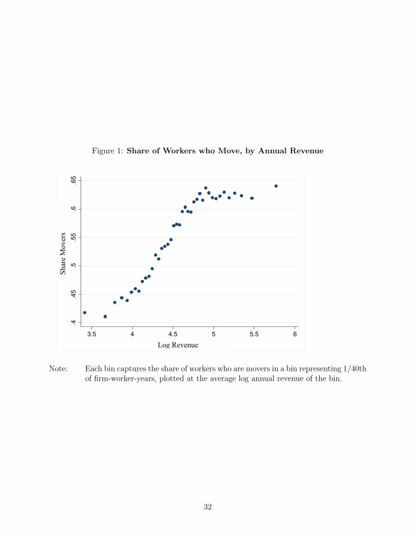
Figure 1: Share of Workers who Move, by Annual Revenue
51
Figure 0: Share of Workers who Move, by Annual Revenue
Each bin captures the share of workers who are movers in a bin representing 1/40th of firm-worker-years, plotted at the average log annual revenue of the bin.
.4.4
5.5
.55
.6.6
5m
ove
r
3.5 4 4.5 5 5.5 6ln_grossrev
Log Revenue
Sha
re M
over
s
Note: Each bin captures the share of workers who are movers in a bin representing 1/40thof firm-worker-years, plotted at the average log annual revenue of the bin.
32

Figure 2: Approximate Symmetry in Productivity Changes of Movers isConsistent with Small Match-Specific Productivity
53
Figure 2: Approximate Symmetry in Productivity Changes of Movers is Consistent with Small Match-Specific Productivity
Note: Using the bins and moves described in Figure 1, Figure 2 displays the productivity changes of workers moving “up” quartiles against workers making the symmetric move “down.”
1 to 2, 2 to 1
1 to 3, 3 to 1
1 to 4, 4 to 1
2 to 3, 3 to 2
2 to 4, 4 to 2
3 to 4, 4 to 3
‐0.14
‐0.12
‐0.1
‐0.08
‐0.06
‐0.04
‐0.02
0
0.02
0.04
‐0.04 ‐0.02 0 0.02 0.04 0.06 0.08 0.1 0.12 0.14
Change in Productivity When
Moving Down
Change in Productivity When Moving Up
Note: Figure displays the productivity changes of workers moving “up” quartiles againstworkers making the symmetric move “down.” Firms are binned by average co-worker performance. For each transitioning worker whom we observe two yearsprior to transition to the new firm and for two years at the new firm with nobreaks, we categorize the move by identifying the quartile before and after move.Thus, “1 to 3” movers move from a bottom quartile firm to a 3rd quartile firm.Workers with multiple moves are included multiple times if they meet the inclusionrequirements.
33

Figure 3: Mobility between Top and Bottom Quartile Productivity Firms isConsistent with Exogenous Mobility
52
Figure 1: Mobility between Top and Bottom Quartile Productivity Firms is Consistent with Exogenous Mobility
Note: Firms are binned by average co-worker performance. For each transitioning worker whom we observe two years prior to transition to the new firm and for two years at the new firm with no breaks, we categorize the move by identifying the quartile before and after move. Thus, “1 to 3” movers move from a bottom quartile firm to a 3rd quartile firm. We plot the path of each mover’s productivity before and after the move, by bin. Paths for movers starting in the 1st and 4th quartiles are plotted here. Error bars represent 95% confidence intervals. Workers with multiple moves are included multiple times if they meet the inclusion requirements.
4.2
4.3
4.4
4.5
4.6
4.7
4.8
4.9
5
‐1 Transition 0 1
Log(revenue)
Year Relative to New Firm
Movers from Top and Bottom Quartile Productivity Firms
4 to 4
4 to 3
4 to 2
4 to 1
1 to 4
1 to 3
1 to 2
1 to 1
Note: Figure plots plot the path of each mover’s productivity before and after the move,by bin. See notes to Figure 2.
34

Figure 4: Productivity Decomposition Shows Higher-Ability Assets at LowerValue-added Firms
54
Figure 3: Productivity Decomposition Shows Higher-Ability Assets at Lower Value-added Firms
Bias Corrected:, 0.04***,
0.07∗∗∗, 0.64∗∗∗
Note: Figure 3 displays the firm and worker fixed effects, prior to small sample bias correction from the decomposition of firm and worker effects. Each dot represents the unbias corrected average firm and worker fixed effects in 50 bins of worker fixed effects. The red line is the uncorrected correlation, while the green line reflects bias correction. Bias corrected correlations and variances are reported below the graph. All results are statistically significant at the 1% level. Statistical significance of variance terms follows from the sampling error. Statistical significance of the correlation is derived from estimating the probability that randomly assigned firm and worker effects would have the estimated correlation.
Note: Figure displays the firm and worker fixed effects, prior to small sample bias correc-tion from their decomposition. Each dot represents the unbias corrected averagefirm and worker fixed effects in 50 bins of worker fixed effects. The red line isthe uncorrected correlation, while the green line reflects bias correction. Bias cor-rected correlations and variances are reported below the graph. All results arestatistically significant at the 1% level. Statistical significance of variance termsfollows from the sampling error. Statistical significance of the correlation is de-rived from estimating the probability that randomly assigned firm and workereffects would have the estimated correlation.
35
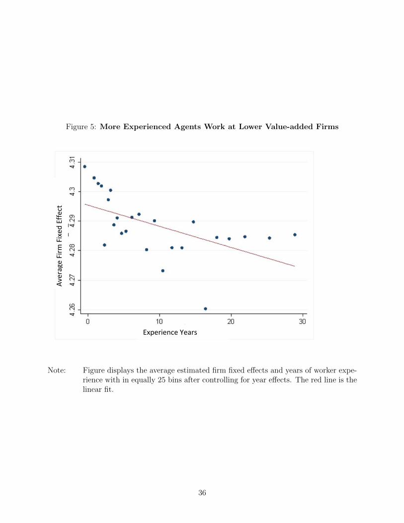
Figure 5: More Experienced Agents Work at Lower Value-added Firms
56
Figure 4: More Experienced Agents Work at Lower Value-added Firms
Note: Figure 4 displays the average estimated firm fixed effects by year of worker experience. 30 reflects 30 or more years of experience. The red line is linearly fit.
Experience Years
Average Firm Fixed
Effect
Note: Figure displays the average estimated firm fixed effects and years of worker expe-rience with in equally 25 bins after controlling for year effects. The red line is thelinear fit.
36

Figure 6: Productivity Decomposition Shows Positive Matching Between Agentsand Firms within Contract Type
58
Figure 5: Productivity Decomposition Shows Positive Matching Between Agents and Firms within Contract Type
Note: We plot assortative matching within specifically identified contract structures. These charts replicate an aggregate matching graph, restricted to workers at firms within specified and identified contract types: “High commission” firms where the contracts offer agents at least 90% of the marginal commission they generate, and traditional commission firms where agents earn approximately 50% of the marginal commission they generate. Each dot represents the unbias corrected average firm and worker fixed effects in 25 bins of worker fixed effects. Red lines are
Note: Figure plots assortative matching within specifically identified contract structures.These charts replicate an aggregate matching graph, restricted to workers at firmswithin specified and identified contract types: “High commission” firms where thecontracts offer agents at least 90% of the marginal commission they generate, andtraditional commission firms where agents earn approximately 50% of the marginalcommission they generate. Each dot represents the unbias corrected average firmand worker fixed effects in 25 bins of worker fixed effects. Red lines are linearlyfit to the unbinned data. Green dashed lines are bias corrected correlations.
37

Figure 7: Mean Residuals are Small and Do Not Vary Systematically
Note: Figure plots mean residuals by decile bins of worker and firm fixed effects. Con-sistent with the estimated functional form assuming log-supermodularity and log-linear production, the mean residuals are small, and do not deviate systematically.Red displays combinations of worker and firm bins which are under predicted bythe estimated complementary production specification, and blue displays regionswhere the the specification over predicts. If the specification fits, there should beno pattern to the colors. If the production technology were less complementarythan the estimated specification, the bottom right quarter of the graph would beblue and the top left would be red.
38

Figure 8: High-Commission Firms Draw More Experienced Workers fromFarther Away and Are Larger and Rare
60
Figure 7: High-Commission Firms Draw More Experienced Workers from Farther Away and Are Larger and Rare
Note: P-values reflect clustering by worker. *** p<0.01, ** p<0.05,* p<0.10. Figure 7 plots the t-tests of characteristics of firms identified as high-commission firms compared to all others. Firm Years shows the split of worker-firm-years by contract type. Distance to office is the distance from the first reported home address to firm address, restricted to workers reporting home addresses within 50 miles of firm offices. Firm size is the average number of workers per year. Experience is the worker experience top-coded at 30.
Firm Years
Other High Commission10
11
12
13
14
15
Other High Commission
Distance to Office(Crow flies miles)***
0
5
10
15
20
25
30
Other High Commission
Firm Size(Workers Per Year)***
8
9
10
11
Other High Commission
Worker Experience(Years)***
Note: P-values reflect clustering by worker. *** p<0.01, ** p<0.05,* p<0.10. Figureplots the t-tests of characteristics of firms identified as high-commission firmscompared to all others. Firm Years shows the split of worker-firm-years by contracttype. Distance to office is the distance from the first reported home address tofirm address, restricted to workers reporting home addresses within 50 miles offirm offices. Firm size is the average number of workers per year. Experience isthe worker experience top-coded at 30.
39

Figure 9: High-Commission Firms Offer Fewer Resources
62
Figure 8: High-Commission Firms Offer Fewer Resources
Note: T-tests as in Figure 7. See notes to Table 4 for variable construction. Robust standard errors are clustered by worker. *** p<0.01, ** p<0.05,* p<0.10.
1.8
1.82
1.84
1.86
1.88
1.9
1.92
Other High Commission
Firm Fixed Effect
‐0.5
0
0.5
1
1.5
Other High Commission
Firm Input Rating (e.g., training) (Survey Rating,
Standardized)***
‐1.5
‐1
‐0.5
0
0.5
1
Other High Commission
Office Leads Rating (Survey Rating, Standardized)**
Note: T-tests as in Figure 8. See notes to Table 5 for variable construction. Robuststandard errors are clustered by worker. *** p<0.01, ** p<0.05,* p<0.10.
40
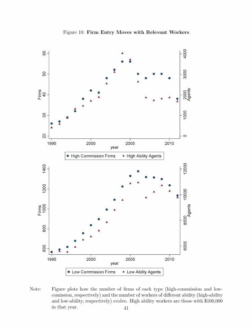
Figure 10: Firm Entry Moves with Relevant Workers
63
Figure 9: Entry and Exit of Firms by Contract Type Respond to Relevant Worker Distributions
Note: Figure 9 plots how the number of firms of each type (high-commission and low-comission, respectively) and the number of workers of different ability (high-ability and low-ability, respectively) evolve. High ability workers are those with $100,000 in that year.
Note: Figure plots how the number of firms of each type (high-commission and low-comission, respectively) and the number of workers of different ability (high-abilityand low-ability, respectively) evolve. High ability workers are those with $100,000in that year. 41

Figure 11: High-Commission Firms Capture a Disproportionate, but Moderate,Share of High-Ability Agents
66
Figure 10: High-Commission Firms Capture a Disproportionate, but Moderate, Share of High-Ability Agents
Note: Figures 10 plots the Lowess fitted firm choice by gross revenue.
10000 100000 1000000 Gross Revenue
Workers
Firms‐Jobs
Note: Figure plots lowess fitted firm choice by gross revenue.
42

Figure 12: Agents’ Distance to First Firm Reflects Spatial Heterogeneity
67
Figure 11: Agents’ Distance to First Firm Reflects Spatial Heterogeneity
Note: Figure 11 plots the smoothed density of distance of workers’ first address to first firm.
Note: Figure plots the smoothed density of distance of workers’ first address to first firm,limited to hose workers within 50 miles.
43
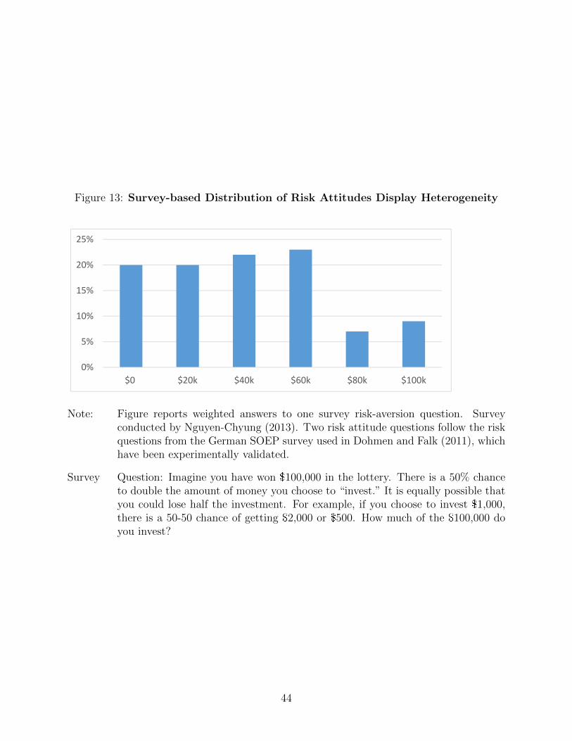
Figure 13: Survey-based Distribution of Risk Attitudes Display Heterogeneity
68
Figure 12: Survey-based Distribution of Risk Attitudes Display Heterogeneity
Survey Question: Imagine you have won $100,000 in the lottery. There is a 50% chance to double the amount of money you choose to “invest.” It is equally possible that you could lose half the investment. For example, if you choose to invest $1,000, there is a 50-50 chance of getting $2,000 or $500. How much of the $100,000 do you invest?25
Note: Figure 12 reports weighted answers to one survey risk-aversion question.
25 Survey conducted by Nguyen-Chyung (2013). Two risk attitude questions follow the risk questions from the German SOEP survey used in Dohmen and Falk (2011), which have been experimentally validated.
0%
5%
10%
15%
20%
25%
$0 $20k $40k $60k $80k $100k
Note: Figure reports weighted answers to one survey risk-aversion question. Surveyconducted by Nguyen-Chyung (2013). Two risk attitude questions follow the riskquestions from the German SOEP survey used in Dohmen and Falk (2011), whichhave been experimentally validated.
Survey Question: Imagine you have won $100,000 in the lottery. There is a 50% chanceto double the amount of money you choose to “invest.” It is equally possible thatyou could lose half the investment. For example, if you choose to invest $1,000,there is a 50-50 chance of getting $2,000 or $500. How much of the $100,000 doyou invest?
44

Figure 14: Benefit of Switching to High-Commission Firms Varies with RiskAversion
69
Figure 13: Benefit of Switching to High-Commission Firms Varies with Risk Aversion
Note: Figure 13 provides a non-parametric estimate of the benefit of switching contracts for different risk-aversion parameters. For each coefficient of relative risk aversion, the lines represent Lowess smoothed plots of the difference in realized utility of workers under different contracts by previous year gross revenue.
Note: Figure provides a non-parametric estimate of the benefit of switching contractsfor different risk-aversion parameters. For each coefficient of relative risk aversion,the lines represent Lowess smoothed plots of the difference in realized utility ofworkers under different contracts by previous year gross revenue.
45

Figure 15: Agent Industry Exits Reflect Uncertainty About Own Ability
70
Figure 14: Agent Industry Exits Reflect Uncertainty About Own Ability
Note: Figure 14 shows the probability of exit (having no sales in the following year), depending on experience.
Probability Of Exit
Experience (Years)
Note: Figure shows the probability of exit (having no sales in the following year), de-pending on experience.
46

Figure 16: Timing of Agent Switching to High-Commission Firms Reflect BothLearning and Other Heterogeneity
71
Figure 15: Timing of Agent Switching to High-Commission Firms Reflect Both Learning and Other Heterogeneity
Note: Conditional on switching to a high-commission firm, Figure 15 plots the share of workers who switch in that year of experience, adjusted for truncation in the panel.
Year at Switch to High Commission
Share Of Switchers
Note: Figure plots the share of workers who switch in that year of experience conditionalon switching to a high-commission firm, adjusted for truncation in the panel.
47
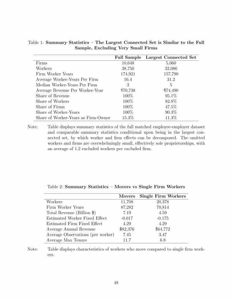
Table 1: Summary Statistics – The Largest Connected Set is Similar to the FullSample, Excluding Very Small Firms
Full Sample Largest Connected SetFirms 10,648 5,060Workers 38,750 32,086Firm Worker Years 174,921 157,790Average Worker-Years Per Firm 16.4 31.2Median Worker-Years Per Firm 3 5Average Revenue Per Worker-Year $70,738 $74,490Share of Revenue 100% 95.1%Share of Workers 100% 82.8%Share of Firms 100% 47.5%Share of Worker-Years 100% 90.3%Share of Worker-Years as Firm-Owner 15.3% 11.3%
Note: Table displays summary statistics of the full matched employee-employer datasetand comparable summary statistics conditional upon being in the largest con-nected set, by which worker and firm effects can be decomposed. The omittedworkers and firms are overwhelmingly small, effectively sole proprietorships, withan average of 1.2 excluded workers per excluded firm.
Table 2: Summary Statistics – Movers vs Single Firm Workers
Movers Single Firm WorkersWorkers 11,708 20,378Firm Worker Years 87,282 70,814Total Revenue (Billion $) 7.19 4.59Estimated Worker Fixed Effect -0.017 -0.175Estimated Firm Fixed Effect 4.29 4.29Average Annual Revenue $82,376 $64,772Average Observations (per worker) 7.45 3.47Average Max Tenure 11.7 6.8
Note: Table displays characteristics of workers who move compared to single firm work-ers.
48

Table 3: Two Stage Least Squares Bias Correction Shows Higher Ability Assetsat Lower Value-added Firms
OLS-FullSample
OLS - WorkerObservables
First Stage 2SLS
DependentVariable
Firm FE Firm FE Worker FE Firm FE
Worker FE -0.100*** -0.102*** -0.076**[0.004] [0.005] [0.037]
San Diego Exam 0.294***[0.031]
Year Fixed Effects Yes Yes Yes YesObservations 157,790 113,129 113,129 113,129Kleibergen-PaapWald F-Stat
89.6
Note: Robust standard errors are clustered by worker and reported in brackets. ***p<0.01, ** p<0.05,* p<0.10. Column (1) regresses the firm fixed effects on theworker fixed effects in the full estimation sample. Column (2) repeats the analysisbut is restricted to the set of workers for whom exam information is available.Column (3) reports the first stage for worker fixed effects using as the excludedinstrument whether one has taken the exam in San Diego. Column (4) reportsthe second stage.
Table 4: More Experienced Agents Work at Lower Valued-added Firms
OLS OLS OLSDependent Variable Firm FE Firm FE Log(Revenue)Worker Experience -0.001*** -0.006*** 0.023***
[<0.0005] [0.003] [0.002]
Year Fixed Effects No Yes YesWorker Fixed Effect No Yes NoWorker X Firm Fixed Effects No No YesObservations 157,790 113,129 113,129
Note: Robust standard errors are clustered by worker and reported in brackets. ***p<0.01, ** p<0.05,* p<0.10. Column (2) adds year fixed effects and worker fixedeffects. Column (3) uses log (revenue) as the dependent variable and includesworker cross firm fixed effects, estimating the increase in revenue for each year ofexperience.
49

Table 5: Survey Measures of Firm Resources Closely Capture Estimated FirmFixed Effects
OLS OLSDependent Variable log(revenue) log(revenue)Firm Fixed Effect 1.001***
[0.006]Office Leads 0.430*** 0.001
[0.067] [0.044]Franchise Inputs (e.g. Training) 0.322*** -0.004
[0.055] [0.035]
Worker Fixed Effect Yes YesExperience Fixed Effects Yes YesYear Fixed Effects Yes Yes
Adjusted With-in Worker R-squared 0.567 0.600Observations 157,790 113,129
Note: Robust standard errors are clustered by firm and reported in brackets. *** p<0.01,** p<0.05,* p<0.10. The survey we used provides two measures of firm resources:“Office Leads” and “Franchise inputs, e.g., training”. Each represents the rateat which survey respondents report either reason as contributing to their success.We aggregate these responses up to a brand level. Log(revenue) is the dependentvariable. Column (2) adds estimated firm fixed effect. Log(Investment) is themedian reported expected investment by national franchise.
Table 6: Expected Franchisee Investments are Correlated with FirmPerformance Measures
OLS OLS OLSDependent Variable Firm FE Franchise Input
RatingOffice Lead
Ratinglog(Investment) 0.012 0.133*** 0.032
[0.015] [0.036] [0.045]
Observations 59,471 59,471 59,471
Note: Robust standard errors are clustered by firm and reported in brackets. *** p<0.01,** p<0.05,* p<0.10. Restricted to national franchises with collected investmentdata.
50

Table 7: Worker Mobility Decisions Reflect Preferences for Firm Resources andLocation
Logit Logit LinearProbability
LinearProbability
LinearProbability
DependentVariable
Move Move Move Move Move
Firm FixedEffect
-1.51*** -1.61*** -0.16*** -0.64*** -0.64***[0.33] [0.32] [0.03] [0.08] [0.08]
Office Leads 0.03 0.15 0.01 0.19*** 0.21***[0.19] [0.18] [0.02] [0.04] [0.04]
Franchise Inputs(e.g. Training)
-1.56*** -1.30*** -0.17*** -0.26*** -0.19***[0.08] [0.08] [0.01] [0.02] [0.02]
Distance (100miles)
0.40*** 0.33*** 0.05*** 0.07*** 0.07***[0.06] [0.06] [0.01] [0.03] [0.03]
Worker FixedEffect
No No No Yes Yes
ExperienceFixed Effects
No Yes No No Yes
Year FixedEffects
No Yes No No Yes
Observations 105,685 105,685 105,685 105,685 105,685
Note: Robust standard errors are clustered by firm and reported in brackets. *** p<0.01,** p<0.05,* p<0.10. This analysis is restricted to workers for whom distance datais available and whose first reported addres sis within 50 miles of their first office.Columns (1) and (2) are logit models of whether a worker moves. Columns 3-5are linear probability models, allowing for worker fixed effects in Columns (4) and(5).
Table 8: Worker’ Firm Choices Reflect Appropriatness of Contract
LogitDependent Variable New firm is high-commissionWage Difference ($ millions) 4.41***
[1.13]
Observations 14,434
Note: The dependent variable is whether the new firm is high-commission, conditionalupon a worker switching firms. The wage difference is the estimated differencein wages between high- and low-commission firms. Robust standard errors areclustered by worker and reported in brackets. *** p<0.01, ** p<0.05,* p<0.10.
51