Competence Effects for Choices involving Gains and Losses

Jose Guilherme de Lara Resende∗ George Wu†

November 30, 2009

Abstract

We investigate how choices for uncertain gain and loss prospects are affected by perceptions of knowl-

edge about the underlying domain of uncertainty. Specifically, we test whether Heath and Tversky’s

(1991) competence hypothesis extends from gains to losses. We predict that the commonly-observed

preference for high knowledge over low knowledge prospects for gains reverses for losses. We employ an

empirical setup in which participants make hypothetical choices between gain or loss prospects in which

the outcome depends on whether a high knowledge or low knowledge event occurs. We infer decision

weighting functions for high and low knowledge events from choices using a representative agent prefer-

ence model. For decisions involving gains, we replicate the results of Kilka and Weber (2001), finding

that decision makers are more attracted to choices that they feel more knowledgeable about. However,

for decisions involving losses, we find limited support for our extension of the competence effect.

Keywords: Uncertainty; Decision Weighting Function; Ambiguity; Knowledge; Competence Effect;

Gains; Losses

JEL classification: C91, D81

∗Universidade de Brasılia, Departamento de Economia - Campus Universitario Darcy Ribeiro, ICC Ala NorteCaixa Postal 04587, Brasılia, DF, Brazil - 70919-970. Tel. 55-61-8137-9225. E-mail: jglresende@unb.br. URL:http://www.unb.br/face/eco/jglresende/†Corresponding Author: University of Chicago, Booth School of Business, 5807 S. Woodlawn Avenue, Chicago, IL 60637.

E-mail: wu@chicagobooth.edu. URL: http://faculty.chicagobooth.edu/george.wu/

1

Decision makers often express a preference for betting on a particular source of uncertainty over another.

Ellsberg (1961) provided the first and most famous demonstration of such a source preference. Ellsberg’s

simple setup involved two urns: a “clear” urn with 50 red balls and 50 black balls, and a “vague” urn with

an unknown proportion of red and black balls (see also Keynes, 1921). Most individuals prefer to bet on the

clear urn over the vague urn, even when they believe that the probability of drawing a red or black ball from

either urn is identical (Becker and Brownson, 1964). Under the classical model of decision under uncertainty,

subjective expected utility (SEU) (Savage, 1954), subjective probabilities are inferred from preferences over

bets. Thus, the typical Ellsberg preferences are inconsistent with the Savage axioms, as these choices reveal

that the subjective probabilities of both red and black are higher for the clear urn than the vague urn.

A large body of subsequent empirical research has explored numerous variants of this demonstration (for a

review, see Camerer and Weber, 1992). The general conclusion of many of these studies, that individuals are

ambiguity averse or reluctant to bet on vague probabilities, has been qualified by several recent studies. Heath

and Tversky (1991) proposed and provided empirical support for the competence hypothesis: decision makers

prefer to bet on ambiguous events over chance events when they consider themselves to be knowledgeable

about the underlying domain of uncertainty (see also Frisch and Baron, 1988). In one study, Heath and

Tversky recruited participants who were experts in either football or politics and non-expert in the other

domain. Participants provided subjective probability assessments of future events involving both political

events and football games. They then indicated their preferences for a chance lottery, a lottery based on

the outcome of a football game, and a lottery based on the outcome of a political event. The lotteries

were matched so that the participant’s subjective likelihood of winning was identical in all cases. The

results showed a source preference consistent with the competence hypothesis. Football experts ranked the

lotteries in order: football, then chance, and finally politics. In contrast, political experts preferred politics

to chance, and chance to football. This pattern of choices reflects a source preference, in which individuals

are ambiguity seeking when they view themselves to be competent or knowledgeable about the underlying

domain of uncertainty and ambiguity averse if the opposite is true.

The present investigation tests whether the competence effect reflects from gains to losses, as originally

posited by Tversky and Wakker (1995). In particular, Tversky and Wakker (1995) hypothesized that par-

ticipants prefer betting on the low knowledge source over the high knowledge source in the domain of losses.

The intuition for this reversal and hence the source preference hypothesis outlined in the next section is that

people shy away from gambles when they feel more confident about the loss they will face (see, e.g., Basili,

Chateauneuf, and Fontini, 2005). In this sense, we predict that preferences will reflect for decision under

uncertainty, as they generally do for decision under risk (e.g., Tversky and Kahneman, 1992).

2

We test this generalization of the competence hypothesis using a variant of one of Heath and Tversky’s

studies. Participants make a series of choices between pairs of gambles that differ on knowledge (high or

low) and domain (gain or loss). Participants also choose between the complements of these gambles. We

fit four probability weighting functions to these data, separately for high knowledge gains, low knowledge

gains, high knowledge losses, and low knowledge losses. For choices involving gains, we replicate Kilka and

Weber’s results, finding that decision makers prefer high knowledge gambles to low knowledge gambles. For

choices involving losses, we find little support for our extension of the competence hypothesis. There is a

significant preference for low versus high knowledge for 1 of our 6 loss tests (and a marginal preference for

another test), but the probability weighting functions estimated for low and high knowledge gambles are not

significantly different. Thus, the competence effect for choices involving losses appears to be less reliable

than the competence effect for gains.

Our paper makes one additional contribution. Our empirical study uses direct choices rather than

certainty equivalents, as used by Tversky and Fox (1995) and Kilka and Weber (2001) and thus investigates

the robustness of Kilka and Weber’s findings to alternative choice procedures. Certainty equivalents are

traditionally used when utility and weighting functions are estimated because they provide considerably more

information than binary choices. However, participants find providing direct certainty equivalents extremely

difficult, and choice-based elicitation of certainty equivalents is tedious (see, e.g., Fischer, Carmon, Ariely,

and Zauberman, 1999). This procedure, therefore, involves a tradeoff: it is relatively straightforward for

participants, but lacks the power to examine individual differences as was done in Abdellaoui, Vossman, and

Weber (2005).

The remainder of the paper is organized as follows. Section 1 reviews previous research on ambiguity.

We also review cumulative prospect theory, Fox and Tversky’s (1995) two-stage model, and describe the

hypothesis we test. Section 2 presents the experimental study. Section 3 discusses the results. We conclude

in Section 4.

1 Background

1.1 Literature

A number of studies have refined the competence hypothesis. Fox and Tversky (1995) suggested that

the feeling of competence or incompetence arises from a comparison of one’s knowledge about an event

with either one’s knowledge about another event or another person’s knowledge of the same event. Thus,

the feeling of knowledge reflects an inherently comparative process. One implication of their comparative

3

ignorance hypothesis is that the classic Ellsberg preferences for the clear urn over the vague urn should

be significantly diminished if participants evaluate the vague and clear urns in isolation. Consistent with

this prediction, Tversky and Fox replicated the classic Ellsberg preferences when participants priced the

vague and clear bets in a within-subject design but found no ambiguity aversion when the two bets were

presented in a between-subject study. Using a similar setup, Chow and Sarin (2001) found significant

between-subject and within-subject price differences. Nevertheless, ambiguity aversion was significantly

weaker in the comparative condition than the non-comparative condition. In another study, Fox and Tversky

documented how an interpersonal comparison might influence the feeling of competence. San Jose State

University undergrads were much less willing to choose an uncertain financial prospect when they were

told that the same prospect was being evaluated by more knowledgeable individuals, graduate students

in economics at Stanford University and professional stock analysts (see also, Fox and Weber, 2002). See

(2009), Taylor (1995), and Trautman, Vieider, and Wakker (2008) provide other psychological accounts of

ambiguity aversion.

A number of theoretical models have been proposed to accommodate ambiguity aversion (see Camerer

and Weber, 1992). A particularly useful formulation for modeling source preference was proposed by Gilboa

(1987) and Schmeidler (1989). These models, termed Choquet expected utility, relax the Savage axioms to

permit nonadditivity of subjective probabilities. Savage’s Sure Thing Principle then no longer applies to

all acts, but only to the subset of acts that are “comonotonic,” i.e., that share the same weak ranking of

states. Choquet expected utility permits nonadditive probability measures, replacing the standard subjective

expected utility calculus with a scheme that involves Choquet integration (Choquet, 1954).1

Tversky and Kahneman’s (1992) cumulative prospect theory (CPT) extended Choquet integration to

permit sign-dependence. Under cumulative prospect theory, the value of a mixed prospect involving the

possibility of gains as well as the possibility of losses is the sum of Choquet integrals of the gain and loss

portions of the prospect. Cumulative prospect theory also extended the scope of Kahneman and Tversky’s

(1979) original prospect theory from prospects with at most two non-zero outcomes to prospects with multiple

outcomes, and from decision under risk (prospects with objective probabilities) to decision under uncertainty

(prospects defined on events). The representation for decision under risk uses a rank-dependent expected

utility form for both gains and losses (Quiggin, 1982). In rank-dependent models, the weight attached to an

outcome depends on the rank of the outcome relative to other outcomes. See Wakker (1990) for a detailed

discussion of the relationship between rank-dependent utility and Choquet expected utility.1Machina (2009) presented a four-color generalization of the Ellsberg Paradox that violates expected utility, as well as

Choquet expected utility. Baillon, l’Haridon, and Placido (2008) showed that this counter-example violates most existingmodels of ambiguity as well.

4

Tversky and Kahneman (1992) also scaled prospect theory for decision under risk, assuming parametric

forms for the value function and probability weighting function. Tversky and Fox (1995) extended the

measurement of prospect theory to decision under uncertainty and proposed a two-stage model. Consider a

lottery in which the decision maker wins x if event E occurs. The two-stage model posits that individuals

first judge the probability of event E, then transform this subjective probability by the probability weighting

function for risk (see also Fox and See, 2003; Fox and Tversky, 1998; Wu and Gonzalez, 1999). The two-

stage model proposed by Tversky and Fox, however, does not permit source preference, and thus cannot

accommodate the Ellsberg Paradox. To deal with this shortcoming, Kilka and Weber (2001) extended

the two-stage model, allowing the transformation of subjective probabilities to depend on the source of

uncertainty. They elicited certainty equivalents for uncertain prospects involving two different sources of

uncertainty, a more and a less familiar source. The certainty equivalents were consistent with Heath and

Tversky’s competence hypothesis. Kilka and Weber estimated significantly different probability weighting

functions for the two sources, with the weighting function more elevated when the source was more familiar.

This paper investigates how choices for gain and loss prospects are affected by the level of knowledge

one has about the decision being made. Numerous studies have shown differences in choices for gains

and losses. Kahneman and Tversky (1979) documented a reflection effect for decision under risk. Most

participants preferred $3000 for sure to an 80% chance at $4000, but preferred an 80% chance at losing

$4000 to losing $3000 for sure. Consistent with this reflection effect, Tversky and Kahneman (1992) estimated

nearly identical value and weighting functions for gains and losses, though subsequent studies have shown

significant differences between gain and loss weighting functions (e.g., Abdellaoui, 2000; Etchart-Vincent,

2004). Several studies have extended the Ellsberg Paradox from gains to losses. These studies have produced

mixed results, with some studies showing ambiguity seeking for losses, particularly for high probability losses

(Cohen, Jaffray and Said, 1985; Einhorn and Hogarth, 1986; Hogarth and Einhorn, 1990; Kahn and Sarin,

1988). Most recently, Abdellaoui, Vossman, and Weber (2005) elicited decision weights for gains and losses

under uncertainty and found that the weighting function for losses was significantly more elevated than the

weighting function for gains.

1.2 Preliminaries

We use cumulative prospect theory (CPT) as our theoretical framework, since it permits a differential

treatment of gains and losses. Under CPT, preferences for uncertain prospects are represented by a value

function v : R → R defined for changes in wealth, and by a decision weighting function or capacity W :

2S → [0, 1] defined on the events under consideration, where S represents the (finite) state space and 2S is

5

the collection of all events. Let Ac, as well as S − A, denote the complement of event A, i.e., A and Ac

are disjoint and A ∪ Ac = S. Let A and B represent two distinct families of events that are each closed

under union and complementation. Each family represents a distinct source of uncertainty. For example,

the final point differential of a football game and the noon temperature in Chicago constitute two sources

of uncertainty.

Let (A, x) denote a prospect that provides x if event A happens and 0 otherwise. (A, x) is a positive

prospect if the prospect involves a gain (i.e., x > 0) and a negative prospect if a loss is possible (i.e., x < 0).

Under CPT,

(A, x) � (B, y)⇐⇒W i(A)v(x) ≥W i(B)v(y),

where i is equal to “+” if (A, x) is a positive prospect and “−” if (A, x) is a negative prospect. Thus, the

decision weighting function W is sign-dependent.

The value function v is defined on changes of wealth, in contrast to expected utility and subjective

expected utility, which are most commonly defined on wealth levels directly. The function is normalized

such that v(0) = 0. Empirical studies have found that v is most commonly concave for gains, convex for

losses and is steeper for losses than for gains (i.e., v exhibits loss aversion) (Abdellaoui, Bleichrodt, and

Paraschiv, 2007; Tversky and Kahneman, 1992).

The decision weighting function satisfies two properties: i) W i(∅) = 0 and W i(S) = 1, where ∅ denotes

the empty set, and S denotes the state space; and ii) W i(A) ≤ W i(B), ∀A ⊂ B. Therefore, W i does not

need to be additive, as is the case with subjective expected utility. Indeed, studies of decision making under

uncertainty have shown that the decision weighting function is typically a non-additive function (e.g., Kilka

and Weber, 2001; Tversky and Fox, 1995; Wu and Gonzalez, 1999).

We now present some properties of the decision weighting function that have been documented in previous

empirical studies.

Definition 1: A decision maker’s weighting function W i displays bounded subadditivity (SA) for the source

A if the two conditions below are satisfied for all A,A′ ∈ A:

i) Lower subadditivity (LSA): W i(A) ≥W i(A ∪A′)−W i(A′), when W i(A ∪A′) is bounded away from 1;

ii) Upper subadditivity (USA): 1−W i(S −A) ≥W i(A∪A′)−W i(A′), when W i(A′) is bounded away from

0.

Intuitively, these conditions mean that the decision maker uses impossibility and certainty as reference

points when choosing. Lower subadditivity (LSA) implies that the impact of an event A is higher when

6

added to the null event (∅) than when it is added to another event A′, provided the two events, A ∪ A′ are

bounded away from one. Upper subadditivity (USA) implies that the impact of an event A is higher when

subtracted from the certain event S than when it is subtracted from another event A ∪ A′, provided that

event A′ is bounded away from zero. Preference conditions for LSA and USA are provided by Tversky and

Wakker (1995), and the basic properties have been documented empirically by Kilka and Weber (2001) and

Tversky and Fox (1995) for gains and Abdellaoui, Vossman, and Weber (2005) for losses.2

We compare decision weighting functions for different sources in order to analyze how knowledge affects

choices. Let A and B be two distinct families of events that correspond to different sources of uncertainty.

For our purposes, we can think of A as a high knowledge source, that is, composed of events which the

decision maker feels more knowledgeable about, and B as a low knowledge source, that is, composed of

events which the decision maker feels less knowledgeable about. We represent general events in A by A,A′,

etc. and general events in B by B,B′, etc. We also assume that events A,A′ (and B,B′) are disjoint.

Tversky and Wakker also proposed a second property of W i(A), termed source sensitivity :

Definition 2: A decision maker displays less sensitivity to source A than to source B in the domain i = +,−

if the two conditions below are satisfied:

i) If W i(A) = W i(B) and W i(A ∪A′) = W i(B ∪B′) then W i(A′) ≥W i(B′), W i(A ∪A′) and W i(B ∪B′)

are bounded away from 1.

ii) If W i(S − A) = W i(S − B) and W i(S − A′) = W i(S − B′) then W i(S − A − A′) ≤ W i(S − B − B′),

W i(S −A−A′) and W i(S −B −B′) are bounded away from 0.

Tversky and Fox (1995) studied source sensitivity by comparing decision weights inferred from choices

involving risk (objective probabilities) and choices involving five domains of uncertainty. They found that

individuals were more sensitive to risk than uncertainty.

We now turn to the property that is the central focus of our paper, source preference (Tversky and

Wakker, 1995):

Definition 3: In the domain of gains, a decision maker displays source preference for source A over source B

if W+(A) = W+(B) implies W+(Ac) ≥W+(Bc), for all A ∈ A and B ∈ B. In the domain of losses, a decision

maker displays source preference for sourceA over source B if W−(A) = W−(B) implies W−(Ac) ≤W−(Bc),

for all A ∈ A and B ∈ B.2Wu and Gonzalez (1999) showed that the weighting function satisfies a stronger property for gains, concavity for low

probability events and convexity for high probability events.

7

For both gains and losses, source preference can be written in preference terms, (A, x) ∼ (B, x) implies

(Ac, x) � (Bc, x) (see Tversky and Wakker, 1995, pp. 1270-1271). Note that the inequality in Definition

3 reverses for losses, since (Ac, x) � (Bc, x) holds for x < 0 if W−(Ac) ≤ W−(Bc). Therefore, source

preference enhances the weighting function for gains and reduces the weighting function for losses. The

Ellsberg two-urns experiment described in the Introduction indicates that people usually display a source

preference for risk over ambiguity when gains are involved. If we denote by E the event of a red ball in the

clear urn and by A the event of a red ball in the vague urn, the standard Ellsberg demonstration shows that

(E, x) � (A, x) and (Ec, x) � (Ac, x).

Next we state our hypothesis about the generalization of the competence effect from gains to losses.

Hypothesis: Decision makers prefer betting on high knowledge domains over low knowledge domains for

gains. However, they prefer betting on low knowledge domains over high knowledge domains for losses.

The gain part of the hypothesis is in accord with the findings of Heath and Tversky (1991) and Kilka and

Weber (2001), with the loss portion previously untested.

Our hypothesis extends Kahneman and Tversky’s original reflection effect (1979) to include source depen-

dence. Kahneman and Tversky showed that preferences are generally risk averse for gains but risk seeking

for losses. For uncertainty, Heath and Tversky’s competence hypothesis asserts that participants tend to

bet on events that they feel more knowledgeable about when choices involve gains. We speculate, however,

that there is an opposite tendency when choices involve losses: participants tend to bet on events that they

feel less knowledgeable about. This is a fundamental behavioral difference between choices with gains and

choices with losses that was not yet investigated.

The basic motivation follows from the fourfold pattern of risk attitudes documented by Tversky and

Kahneman (1992). Decision makers are typically risk averse for medium to high probability gains and risk

seeking for low probability gains. This pattern reverses for losses. Tversky and Fox (1995) suggest that risk

aversion and risk seeking might be explained in part by affective feelings such as fear and hope. Thus, the

medium to high probabilities that produce fear for gains correspond to hope for losses, with low probabilities

resulting in hope for gains and fear for losses. We hypothesize that a similar pattern holds for ambiguity.

High knowledge domains are relatively more hopeful for gains but relatively more fearful for losses.

A similar intuition is expressed in Basili, Chateauneuf, and Fontini (2005). They extend prospect theory,

dividing outcomes into familiar and unfamiliar ones, and propose that preferences reflect pessimism for gains

and optimism for losses when outcomes are unfamiliar. The reason for this reflection from a preference for

high knowledge for gains to low knowledge for losses is straightforward. For sources that differ in competence,

8

it means that people tend to shy away from the certainty of having a loss. Therefore, when choosing between

two uncertain events that differ only in the relative feeling of competence, decision makers choose the one

they feel less competent about.

We quantify our main hypothesis by using the two-stage process originally proposed by Tversky and Fox

(1998) and extended by Kilka and Weber (2001). Tversky and Fox proposed that decision makers evaluate

an uncertain prospect, (A, x), by first judging the probability of the event A and then transforming this

judged probability using a risky weighting function:

W (A) = wR(P (A)),

where W is the weighting function for uncertainty, P (A) is the judged probability for event A, and wR is

the risky weighting function, i.e., the weighting function applied to prospects with objective probabilities.

Tversky and Fox (1995) and Fox and Tversky (1998) provided empirical support for this two-stage model, and

Wakker (2004) offered a formal justification for this approach. However, this account is clearly incompatible

with the Ellsberg Paradox. Thus, Kilka and Weber (2001) extended the two-stage model to account for

source preference:

W (A) = wS(P (A)),

where wS is the weighting function for source S of uncertainty. Source preference and source sensitivity can

be captured with the functional specification originally proposed by Goldstein and Einhorn (1987) for risk:

w(p) =δpγ

δpγ + (1− p)γ. (1.1)

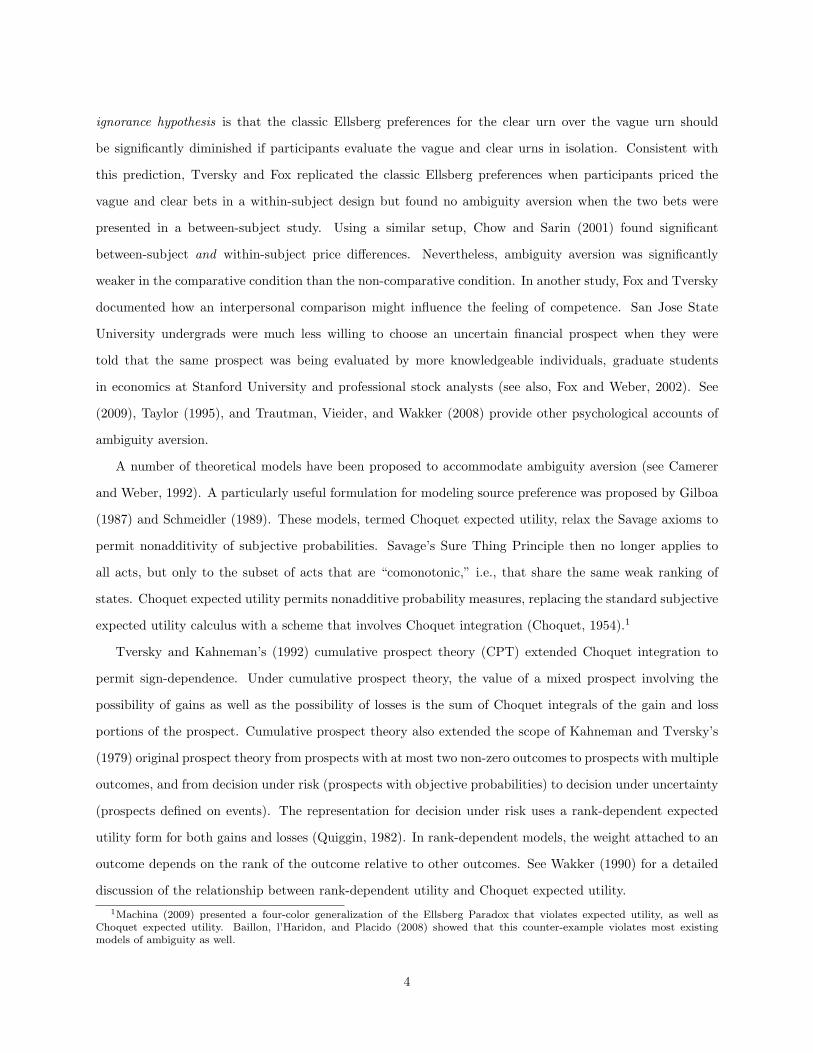
This function was used by Birnbaum and McIntosh (1996), Gonzalez and Wu (1999), Kilka and Weber (2001),

Lattimore et al (1992), and Tversky and Fox (1995), among others. All of the participants in Gonzalez and

Wu (1999) exhibited an inverse S-shaped probability weighting function, such that low probabilities were

overweighted and high probabilities were underweighted. However, there was considerable heterogeneity

across participants, and Gonzalez and Wu showed that this two-parameter function was better able to capture

the heterogeneity than standard one-parameter weighting functions. The weighting function estimates for

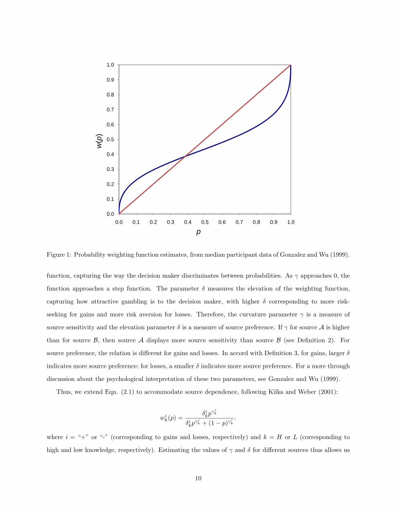
the median data in Gonzalez and Wu (1999) are plotted in Figure 1.

Each parameter, δ and γ, in Eqn. (2.1) captures a different psychological characteristic. Expected utility

corresponds to w(p) = p, or γ = 1 and δ = 1. The parameter γ measures the curvature of the weighting

9

0.0

0.1

0.2

0.3

0.4

0.5

0.6

0.7

0.8

0.9

1.0

0.0 0.1 0.2 0.3 0.4 0.5 0.6 0.7 0.8 0.9 1.0

w(p

)

p

Figure 1: Probability weighting function estimates, from median participant data of Gonzalez and Wu (1999).

function, capturing the way the decision maker discriminates between probabilities. As γ approaches 0, the

function approaches a step function. The parameter δ measures the elevation of the weighting function,

capturing how attractive gambling is to the decision maker, with higher δ corresponding to more risk-

seeking for gains and more risk aversion for losses. Therefore, the curvature parameter γ is a measure of

source sensitivity and the elevation parameter δ is a measure of source preference. If γ for source A is higher

than for source B, then source A displays more source sensitivity than source B (see Definition 2). For

source preference, the relation is different for gains and losses. In accord with Definition 3, for gains, larger δ

indicates more source preference; for losses, a smaller δ indicates more source preference. For a more through

discussion about the psychological interpretation of these two parameters, see Gonzalez and Wu (1999).

Thus, we extend Eqn. (2.1) to accommodate source dependence, following Kilka and Weber (2001):

wik(p) =δikp

γik

δikpγi

k + (1− p)γik

.

where i = “+” or “-” (corresponding to gains and losses, respectively) and k = H or L (corresponding to

high and low knowledge, respectively). Estimating the values of γ and δ for different sources thus allows us

10

to test for source preference. In particular, we can test whether our hypotheses holds, by comparing δ+H and

δ+L , and δ−H and δ−L . Our hypothesis requires that δ+

H > δ+L and δ−H > δ−L .

Finally, following Fox and Tversky (1998), who showed that judged probabilities satisfy support theory

(Tversky and Koehler, 1994), we also test whether judged probabilities satisfy binary complementarity, i.e.,

the probabilities of complementary events sum to one:3

Definition 4: Judged probabilities satisfy binary complementarity for a given source (A) if P (A)+P (Ac) = 1

for all A ∈ A.

Empirical support for binary complementarity is provided by Tversky and Koehler (1994) and Tversky

and Fox (1995). Violations of binary complementarity, however, have been documented by Brenner and

Rottenstreich (1999) and Macchi, Osherson, and Krantz (1999).

2 Experimental Design

We examined source preference for gains and losses by asking participants to make a series of hypothetical

choices between two uncertain prospects, a “high knowledge” (HK) prospect and a “low knowledge” (LK)

prospect. We selected events for the prospects such that most participants would feel more knowledgeable

about the high knowledge prospect than the low knowledge prospect. To illustrate, we expected most of

our University of Chicago student participants to be more familiar and hence more knowledgeable about

Chicago weather than Bucharest weather. Thus, to test for source preference, participants were given a choice

between a “high knowledge” prospect for which they would win $160 if the high temperature in Chicago

was greater than 85◦ Fahrenheit on July 15, 2005 (and $0 otherwise) and a “low knowledge” prospect for

which they would win $160 if the high temperature in Bucharest was greater than 85◦ Fahrenheit on July

15, 2005 (and $0 otherwise). Note that most features of the prospects are identical so as to heighten the

comparative ignorance. The only difference is whether participants preferred to “bet on Chicago” or “bet

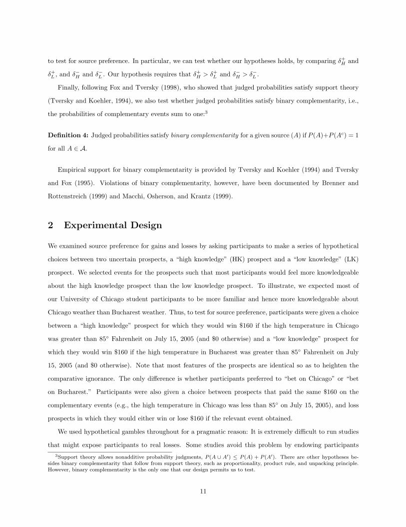
on Bucharest.” Participants were also given a choice between prospects that paid the same $160 on the

complementary events (e.g., the high temperature in Chicago was less than 85◦ on July 15, 2005), and loss

prospects in which they would either win or lose $160 if the relevant event obtained.

We used hypothetical gambles throughout for a pragmatic reason: It is extremely difficult to run studies

that might expose participants to real losses. Some studies avoid this problem by endowing participants3Support theory allows nonadditive probability judgments, P (A ∪ A′) ≤ P (A) + P (A′). There are other hypotheses be-

sides binary complementarity that follow from support theory, such as proportionality, product rule, and unpacking principle.However, binary complementarity is the only one that our design permits us to test.

11

with a generous show-up fee to offset losses incurred in the study (e.g., Cohen, Jaffray, and Said, 1985).

However, this endowment procedure might create a house money effect (see Thaler and Johnson, 1990).

Empirically, reviews have reached different conclusions about whether financial incentives changes behavior.

Camerer and Hogarth (1999) reviewed 74 studies in which performance-based incentives were zero, low, or

high. Although higher incentives seem to improve performance on some tasks (e.g., memory tasks), they

harm performance on other tasks (e.g., difficult tasks for which simple and intuitive heuristics can perform

well). Most critically, Camerer and Hogarth conclude that “(t)here is no replicated study in which a theory

of rational choice was rejected at low stakes in favor of a well-specified behavioral alternative, and accepted

at high stakes.” (p. 33). In contrast, Hertwig and Ortmann (2001) review a number of decision studies

that involve both payment and non-payment conditions. They conclude: ”In the majority of cases where

payments made a difference, they improved peoples performance.” (p. 394)

2.1 Participants

We recruited 107 University of Chicago undergraduate students in May 2005 to participate in our study.

Participation was voluntary, and participants received $3 for participating.

2.2 Procedure

The experiment was entirely computer-based.4 Participants first saw an opening page that provided an

overview of the study. The opening page was followed by an instruction page that explained the subsequent

trials. After the instruction page, participants were given three practice trials, aimed to familiarize them

with the structure of choices and the procedure involved for making these choices. The trials appeared

on their own page, with one choice involving gains, one choice involving losses, and one page involving a

probability assessment.

2.3 Stimuli

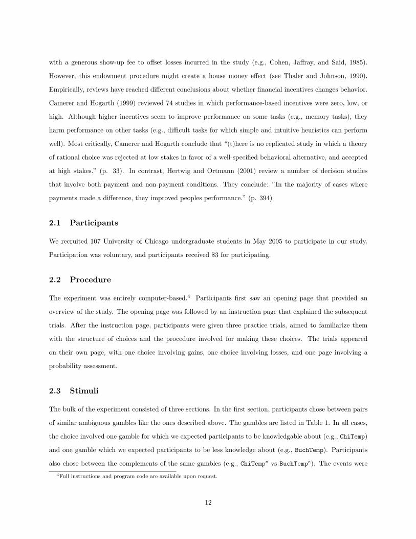
The bulk of the experiment consisted of three sections. In the first section, participants chose between pairs

of similar ambiguous gambles like the ones described above. The gambles are listed in Table 1. In all cases,

the choice involved one gamble for which we expected participants to be knowledgable about (e.g., ChiTemp)

and one gamble which we expected participants to be less knowledge about (e.g., BuchTemp). Participants

also chose between the complements of the same gambles (e.g., ChiTempc vs BuchTempc). The events were

4Full instructions and program code are available upon request.

12

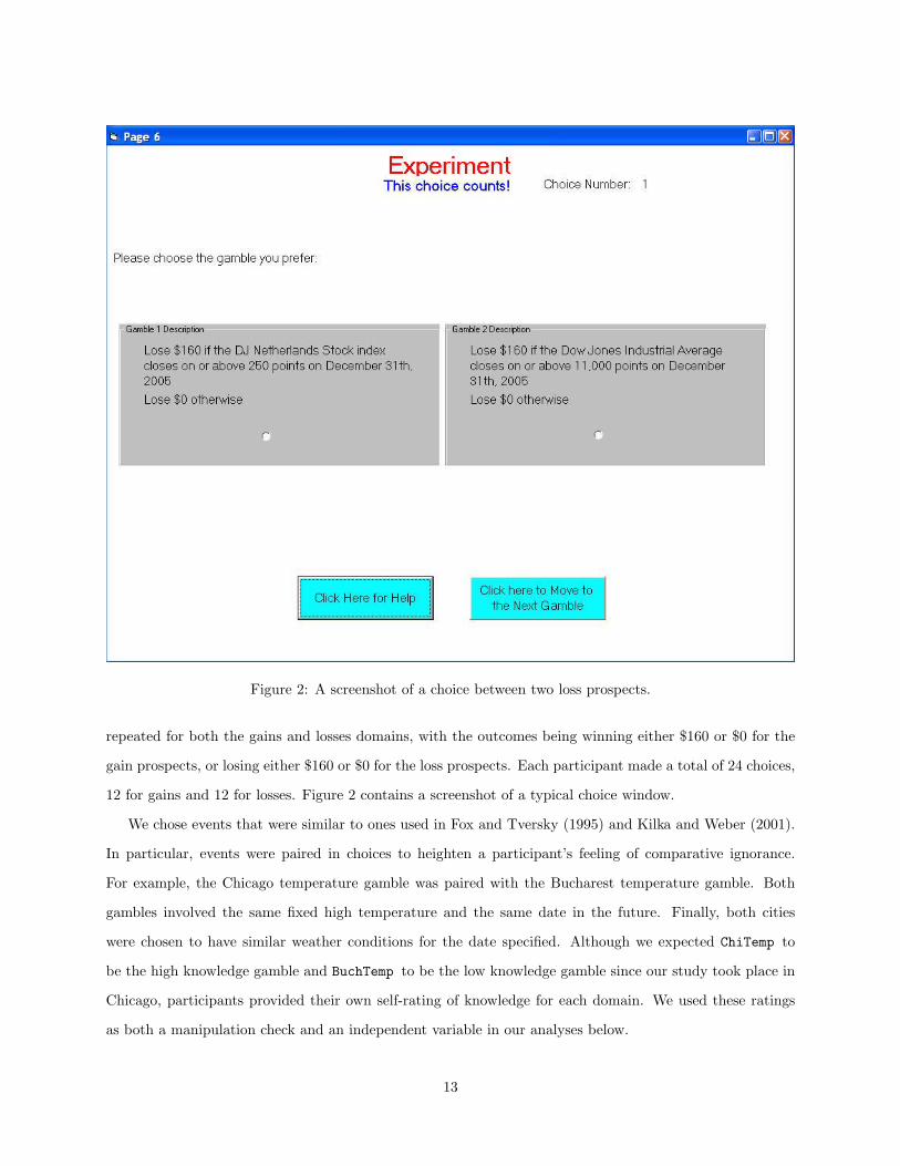
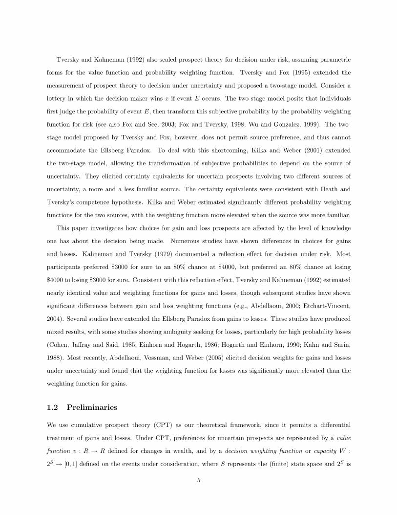
Figure 2: A screenshot of a choice between two loss prospects.

repeated for both the gains and losses domains, with the outcomes being winning either $160 or $0 for the

gain prospects, or losing either $160 or $0 for the loss prospects. Each participant made a total of 24 choices,

12 for gains and 12 for losses. Figure 2 contains a screenshot of a typical choice window.

We chose events that were similar to ones used in Fox and Tversky (1995) and Kilka and Weber (2001).

In particular, events were paired in choices to heighten a participant’s feeling of comparative ignorance.

For example, the Chicago temperature gamble was paired with the Bucharest temperature gamble. Both

gambles involved the same fixed high temperature and the same date in the future. Finally, both cities

were chosen to have similar weather conditions for the date specified. Although we expected ChiTemp to

be the high knowledge gamble and BuchTemp to be the low knowledge gamble since our study took place in

Chicago, participants provided their own self-rating of knowledge for each domain. We used these ratings

as both a manipulation check and an independent variable in our analyses below.

13

ChiTemp High temperature in Chicago is AT LEAST 85F on July 15, 2005BuchTemp High temperature in Bucharest is AT LEAST 85F on July 15, 2005

ChiTempc High temperature in Chicago is AT MOST 85F on July 15, 2005BuchTempc High temperature in Bucharest is AT MOST 85F on July 15, 2005

MH Miami Heat wins next year’s NBA championshipJuve Juventus wins next year’s Italian series A soccer championship

MHc Miami Heat loses next year’s NBA championshipJuvec Juventus loses next year’s Italian series A soccer championship

DJIA The Dow Jones Industrial Average closes BELOW 11,000 points on Dec 31, 2005DJNeth The DJ Netherlands Stock index closes BELOW 250 points on Dec 31th, 2005

DJIAc The Dow Jones Industrial Average closes ON OR ABOVE 11,000 points on Dec 31, 2005DJNethc The DJ Netherlands Stock index closes ON OR ABOVE 250 points on Dec 31th, 2005

USInf The United States inflation rate is BELOW 4% for the 2006 yearSwInf The Swedish inflation rate is BELOW 4% for the 2006 year

USInfc The United States inflation rate is ON OR ABOVE 4% for the 2006 yearSwInfc The Swedish inflation rate is ON OR ABOVE 4% for the 2006 year

USOly The United States wins more than 100 medals in the Olympic Games in Beijing 2008PolOly Poland wins more than 10 medals in the Olympic Games in Beijing 2008

USOlyc The United States wins less than 100 medals in the Olympic Games in Beijing 2008PolOlyc Poland wins less than 10 medals in the Olympic Games in Beijing 2008

ChiSnow Snows more than 1 inch in Chicago on January 10, 2006OsloSnow Snows more than 1 inch in Oslo on January 10, 2006

ChiSnowc Snows 1 inch or less in Chicago on January 10, 2006OsloSnowc Snows 1 inch or less in Oslo on January 10, 2006

Table 1: Uncertain events used for gambles. Gambles were constructed from these uncertain events suchthat for gains, participants won $160 if the event obtained, and for losses, participants lost $160 if the eventobtained.

14

One critical difference between our study and those of Fox and Tversky (1995) and Kilka and Weber

(2001) is that our study involved direct choices, whereas their experiment required participants to assign

cash equivalents to various prospects. We used direct choices because trying to elicit certainty equivalents

would increase enormously the number of choices a typical participant would have to make.

The order of the questions were randomized within section. We also randomized the position of the

gamble in the choice window, left or right (see Figure 2). Finally, to minimize confusion, all the gain

prospects and all the loss prospects were kept together, although we randomized the domain participants

saw first.

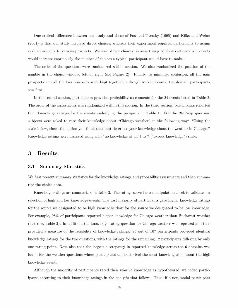
In the second section, participants provided probability assessments for the 24 events listed in Table 2.

The order of the assessments was randomized within this section. In the third section, participants reported

their knowledge ratings for the events underlying the prospects in Table 1. For the ChiTemp question,

subjects were asked to rate their knowledge about “Chicago weather” in the following way: “Using the

scale below, check the option you think that best describes your knowledge about the weather in Chicago.”

Knowledge ratings were assessed using a 1 (“no knowledge at all”) to 7 (“expert knowledge”) scale.

3 Results

3.1 Summary Statistics

We first present summary statistics for the knowledge ratings and probability assessments and then summa-

rize the choice data.

Knowledge ratings are summarized in Table 2. The ratings served as a manipulation check to validate our

selection of high and low knowledge events. The vast majority of participants gave higher knowledge ratings

for the source we designated to be high knowledge than for the source we designated to be low knowledge.

For example, 98% of participants reported higher knowledge for Chicago weather than Bucharest weather

(last row, Table 2). In addition, the knowledge rating question for Chicago weather was repeated and thus

provided a measure of the reliability of knowledge ratings: 95 out of 107 participants provided identical

knowledge ratings for the two questions, with the ratings for the remaining 12 participants differing by only

one rating point. Note also that the largest discrepancy in reported knowledge across the 6 domains was

found for the weather questions where participants tended to feel the most knowledgeable about the high

knowledge event.

Although the majority of participants rated their relative knowledge as hypothesized, we coded partic-

ipants according to their knowledge ratings in the analysis that follows. Thus, if a non-modal participant

15

reported higher knowledge for Italian soccer than U.S. basketball, then we coded Juve as the high knowledge

event and MH as the low knowledge event for that participant.

Table 2: Knowledge Ratings

International Economic Financial InternationalWeather Sports Indicators Markets Sports Weather

High Knowledge (HK)Chicago US BBall US US US Chicago

Average 4.85 3.34 3.20 3.15 3.59 4.83Std Dev 1.14 1.63 1.47 1.38 1.43 1.14

Low Knowledge (LK)Bucharest Ital Soccer Sweden Netherlands Poland Oslo

Average 1.90 2.36 1.74 1.53 1.75 2.21Std Dev 1.08 1.66 0.96 0.88 0.97 1.31

HK Ratings> LK Ratings 98% 84% 98% 95% 95% 100%

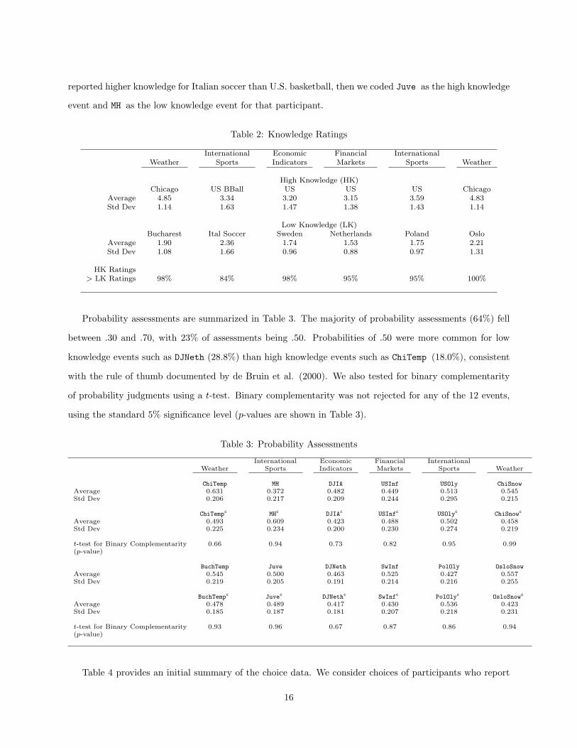
Probability assessments are summarized in Table 3. The majority of probability assessments (64%) fell

between .30 and .70, with 23% of assessments being .50. Probabilities of .50 were more common for low

knowledge events such as DJNeth (28.8%) than high knowledge events such as ChiTemp (18.0%), consistent

with the rule of thumb documented by de Bruin et al. (2000). We also tested for binary complementarity

of probability judgments using a t-test. Binary complementarity was not rejected for any of the 12 events,

using the standard 5% significance level (p-values are shown in Table 3).

Table 3: Probability Assessments

International Economic Financial InternationalWeather Sports Indicators Markets Sports Weather

ChiTemp MH DJIA USInf USOly ChiSnowAverage 0.631 0.372 0.482 0.449 0.513 0.545Std Dev 0.206 0.217 0.209 0.244 0.295 0.215

ChiTempc MHc DJIAc USInfc USOlyc ChiSnowc

Average 0.493 0.609 0.423 0.488 0.502 0.458Std Dev 0.225 0.234 0.200 0.230 0.274 0.219

t-test for Binary Complementarity 0.66 0.94 0.73 0.82 0.95 0.99(p-value)

BuchTemp Juve DJNeth SwInf PolOly OsloSnowAverage 0.545 0.500 0.463 0.525 0.427 0.557Std Dev 0.219 0.205 0.191 0.214 0.216 0.255

BuchTempc Juvec DJNethc SwInfc PolOlyc OsloSnowc

Average 0.478 0.489 0.417 0.430 0.536 0.423Std Dev 0.185 0.187 0.181 0.207 0.218 0.231

t-test for Binary Complementarity 0.93 0.96 0.67 0.87 0.86 0.94(p-value)

Table 4 provides an initial summary of the choice data. We consider choices of participants who report

16

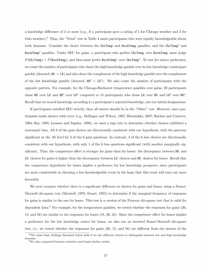
a knowledge difference of 2 or more (e.g., if a participant gave a rating of 5 for Chicago weather and 3 for

Oslo weather).5 Thus, the “Total” row in Table 4 omits participants who were equally knowledgeable about

both domains. Consider the choice between the ChiTemp and BuchTemp gambles, and the ChiTempc and

BuchTempc gambles. Under SEU for gains, a participant who prefers ChiTemp over BuchTemp must judge

P (ChiTemp) > P (BuchTemp), and thus must prefer BuchTempc over ChiTempc. To test for source preference,

we count the number of participants who chose the high knowledge gamble over its low knowledge counterpart

gamble (denoted, HK � LK) and also chose the complement of the high knowledge gamble over the complement

of the low knowledge gamble (denoted, HKc � LKc). We also count the number of participants with the

opposite pattern. For example, for the Chicago-Bucharest temperature gambles over gains, 20 participants

chose HK over LK and HKc over LKc compared to 15 participants who chose LK over HK and LKc over HKc.

Recall that we scored knowledge according to a participant’s reported knowledge, not our initial designations.

If participants satisfied SEU strictly, then all entries should be in the “Other” row. However, since par-

ticipants make choices with error (e.g., Ballinger and Wilcox, 1997; Blavatskky, 2007; Harless and Camerer,

1994; Hey, 1995; Loomes and Sugden, 1998), we used a sign test to determine whether choices exhibited a

systematic bias. All 6 of the gain choices are directionally consistent with our hypothesis, with the patterns

significant at the .05 level for 3 of the 6 gain questions. In contrast, 4 of the 6 loss choices are directionally

consistent with our hypothesis, with only 1 of the 6 loss questions significant (with another marginally sig-

nificant). Thus, the competence effect is stronger for gains than for losses: the discrepancy between HK and

LK choices for gains is higher than the discrepancy between LK choices and HK choices for losses. Recall that

the competence hypothesis for losses implies a preference for low knowledge prospects, since participants

are more comfortable in choosing a less knowledgeable event in the hope that this event will turn out more

favorably.

We next examine whether there is a significant difference in choices for gains and losses, using a Stuart-

Maxwell chi-square test (Maxwell, 1970; Stuart, 1955) to determine if the marginal frequency of responses

for gains is similar to the one for losses. This test is a version of the Pearson chi-square test that is valid for

dependent data.6 For example, for the temperature gambles, we tested whether the responses for gains (20,

15, and 58) are similar to the responses for losses (18, 30, 45). Since the competence effect for losses implies

a preference for the low knowledge source for losses, we also ran an inverted Stuart-Maxwell chi-square

test, i.e., we tested whether the responses for gains (20, 15, and 58) are different from the inverse of the

5The same basic findings discussed below hold if we use different criteria to distinguish between low and high knowledgedomains.

6We also computed Pearson statistics and found similar results.

17

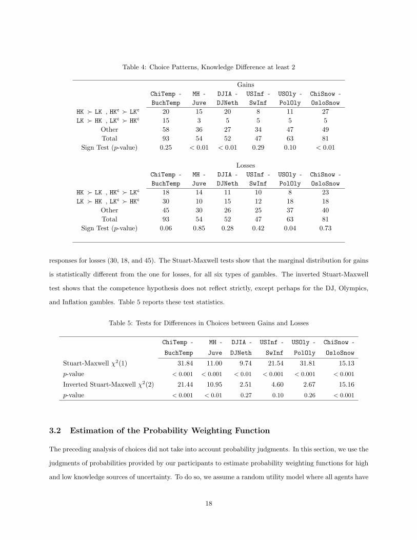
Table 4: Choice Patterns, Knowledge Difference at least 2

GainsChiTemp - MH - DJIA - USInf - USOly - ChiSnow -BuchTemp Juve DJNeth SwInf PolOly OsloSnow

HK � LK , HKc � LKc 20 15 20 8 11 27LK � HK , LKc � HKc 15 3 5 5 5 5

Other 58 36 27 34 47 49Total 93 54 52 47 63 81

Sign Test (p-value) 0.25 < 0.01 < 0.01 0.29 0.10 < 0.01

LossesChiTemp - MH - DJIA - USInf - USOly - ChiSnow -BuchTemp Juve DJNeth SwInf PolOly OsloSnow

HK � LK , HKc � LKc 18 14 11 10 8 23LK � HK , LKc � HKc 30 10 15 12 18 18

Other 45 30 26 25 37 40Total 93 54 52 47 63 81

Sign Test (p-value) 0.06 0.85 0.28 0.42 0.04 0.73

responses for losses (30, 18, and 45). The Stuart-Maxwell tests show that the marginal distribution for gains

is statistically different from the one for losses, for all six types of gambles. The inverted Stuart-Maxwell

test shows that the competence hypothesis does not reflect strictly, except perhaps for the DJ, Olympics,

and Inflation gambles. Table 5 reports these test statistics.

Table 5: Tests for Differences in Choices between Gains and Losses

ChiTemp - MH - DJIA - USInf - USOly - ChiSnow -

BuchTemp Juve DJNeth SwInf PolOly OsloSnow

Stuart-Maxwell χ2(1) 31.84 11.00 9.74 21.54 31.81 15.13

p-value < 0.001 < 0.001 < 0.01 < 0.001 < 0.001 < 0.001

Inverted Stuart-Maxwell χ2(2) 21.44 10.95 2.51 4.60 2.67 15.16

p-value < 0.001 < 0.01 0.27 0.10 0.26 < 0.001

3.2 Estimation of the Probability Weighting Function

The preceding analysis of choices did not take into account probability judgments. In this section, we use the

judgments of probabilities provided by our participants to estimate probability weighting functions for high

and low knowledge sources of uncertainty. To do so, we assume a random utility model where all agents have

18

the same underlying preferences and thus estimate an empirical representative agent (Wilcox, 2008). Similar

procedures have been used in decision under risk by Camerer and Ho (1994), Wu and Gonzalez (1996), and

Wu and Markle (2008) (see also Stott, 2006).

As in Camerer and Ho, we assume that all agents have the same preferences (i.e., decision weighting

and value function). We also assume that the source of uncertainty affects only the probability weighting

function and not the value function. Variation in choices is accounted for by the stochastic part in the

utility function, as well as differences in assessments of the likelihood of the events. Let Ak represent the

ambiguous event, and Gik = (Ak, x) be the uncertain prospect corresponding to the ambiguous event Ak,

where k indexes the source of ambiguity and i=“+” if x > 0 and i =“-” if x < 0. Then, the random utility

model is written as:

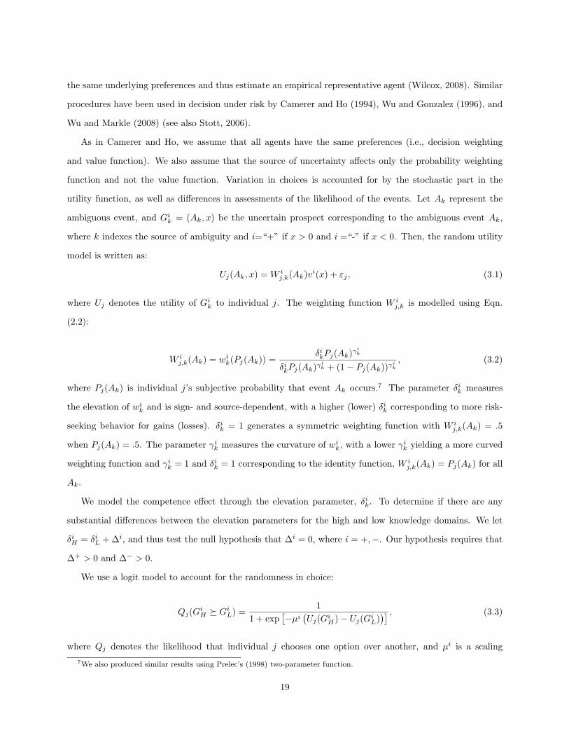
Uj(Ak, x) = W ij,k(Ak)vi(x) + εj , (3.1)

where Uj denotes the utility of Gik to individual j. The weighting function W ij,k is modelled using Eqn.

(2.2):

W ij,k(Ak) = wik(Pj(Ak)) =

δikPj(Ak)γik

δikPj(Ak)γik + (1− Pj(Ak))γi

k

, (3.2)

where Pj(Ak) is individual j’s subjective probability that event Ak occurs.7 The parameter δik measures

the elevation of wik and is sign- and source-dependent, with a higher (lower) δik corresponding to more risk-

seeking behavior for gains (losses). δik = 1 generates a symmetric weighting function with W ij,k(Ak) = .5

when Pj(Ak) = .5. The parameter γik measures the curvature of wik, with a lower γik yielding a more curved

weighting function and γik = 1 and δik = 1 corresponding to the identity function, W ij,k(Ak) = Pj(Ak) for all

Ak.

We model the competence effect through the elevation parameter, δik. To determine if there are any

substantial differences between the elevation parameters for the high and low knowledge domains. We let

δiH = δiL + ∆i, and thus test the null hypothesis that ∆i = 0, where i = +,−. Our hypothesis requires that

∆+ > 0 and ∆− > 0.

We use a logit model to account for the randomness in choice:

Qj(GiH � GiL) =1

1 + exp[−µi

(Uj(GiH)− Uj(GiL)

)] , (3.3)

where Qj denotes the likelihood that individual j chooses one option over another, and µi is a scaling

7We also produced similar results using Prelec’s (1998) two-parameter function.

19

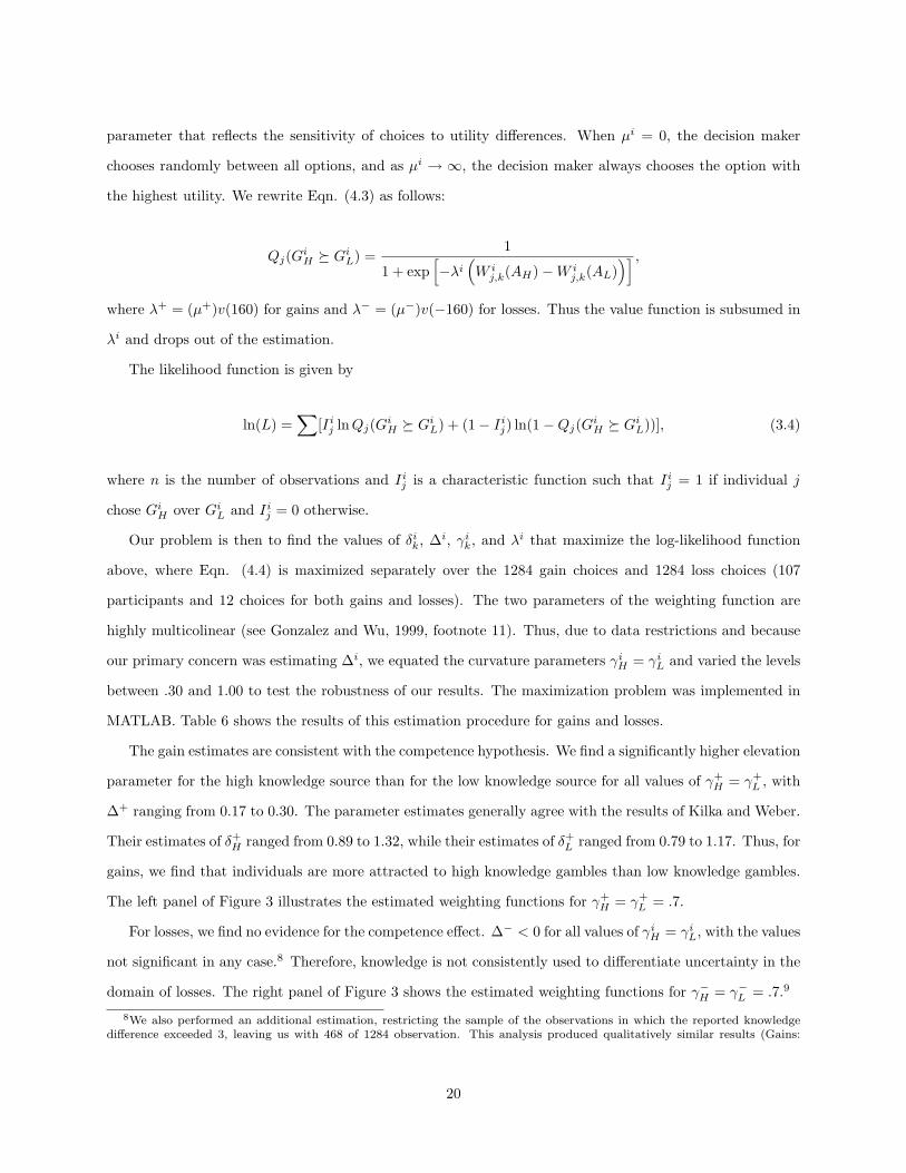
parameter that reflects the sensitivity of choices to utility differences. When µi = 0, the decision maker

chooses randomly between all options, and as µi → ∞, the decision maker always chooses the option with

the highest utility. We rewrite Eqn. (4.3) as follows:

Qj(GiH � GiL) =1

1 + exp[−λi

(W ij,k(AH)−W i

j,k(AL))] ,

where λ+ = (µ+)v(160) for gains and λ− = (µ−)v(−160) for losses. Thus the value function is subsumed in

λi and drops out of the estimation.

The likelihood function is given by

ln(L) =∑

[Iij lnQj(GiH � GiL) + (1− Iij) ln(1−Qj(GiH � GiL))], (3.4)

where n is the number of observations and Iij is a characteristic function such that Iij = 1 if individual j

chose GiH over GiL and Iij = 0 otherwise.

Our problem is then to find the values of δik, ∆i, γik, and λi that maximize the log-likelihood function

above, where Eqn. (4.4) is maximized separately over the 1284 gain choices and 1284 loss choices (107

participants and 12 choices for both gains and losses). The two parameters of the weighting function are

highly multicolinear (see Gonzalez and Wu, 1999, footnote 11). Thus, due to data restrictions and because

our primary concern was estimating ∆i, we equated the curvature parameters γiH = γiL and varied the levels

between .30 and 1.00 to test the robustness of our results. The maximization problem was implemented in

MATLAB. Table 6 shows the results of this estimation procedure for gains and losses.

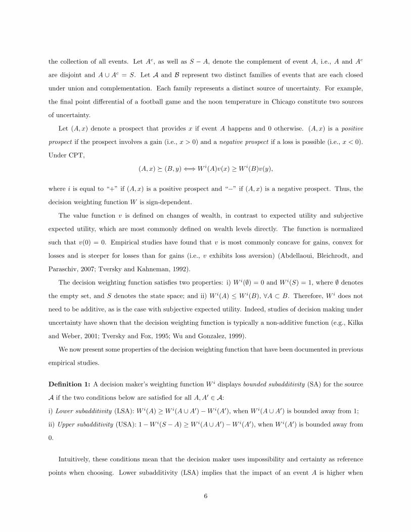
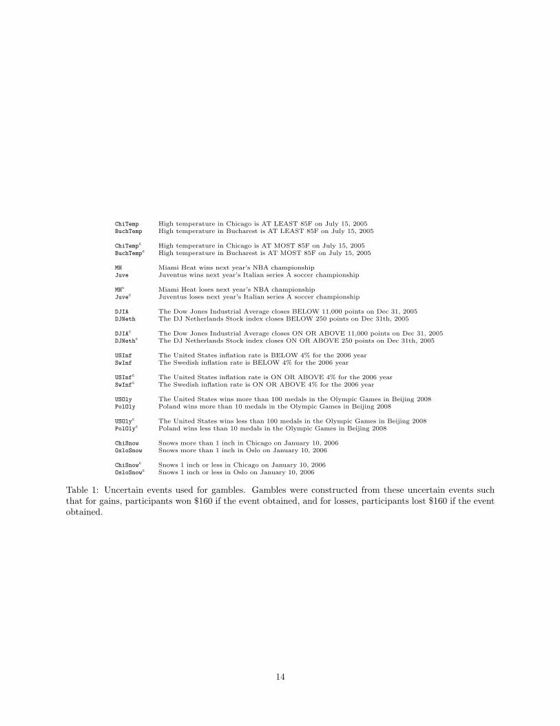
The gain estimates are consistent with the competence hypothesis. We find a significantly higher elevation

parameter for the high knowledge source than for the low knowledge source for all values of γ+H = γ+

L , with

∆+ ranging from 0.17 to 0.30. The parameter estimates generally agree with the results of Kilka and Weber.

Their estimates of δ+H ranged from 0.89 to 1.32, while their estimates of δ+

L ranged from 0.79 to 1.17. Thus, for

gains, we find that individuals are more attracted to high knowledge gambles than low knowledge gambles.

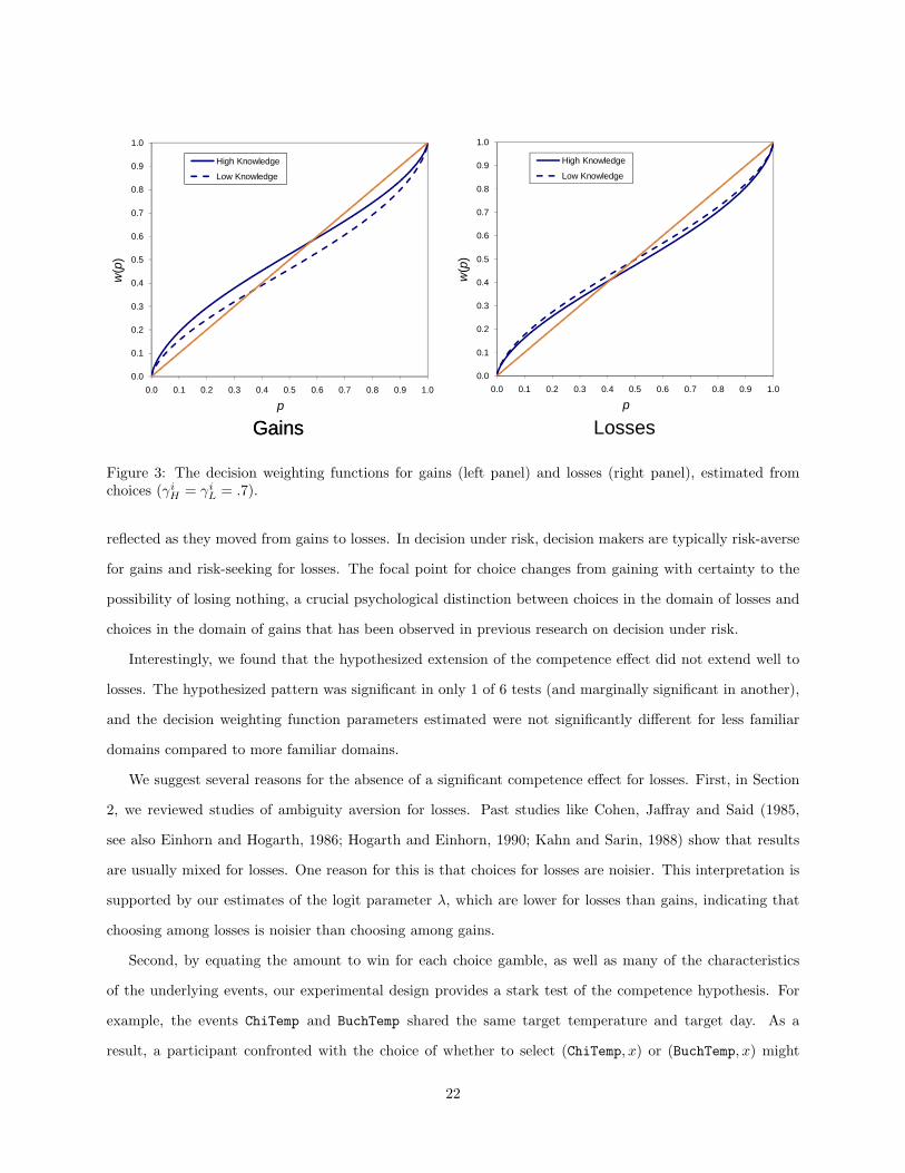
The left panel of Figure 3 illustrates the estimated weighting functions for γ+H = γ+

L = .7.

For losses, we find no evidence for the competence effect. ∆− < 0 for all values of γiH = γiL, with the values

not significant in any case.8 Therefore, knowledge is not consistently used to differentiate uncertainty in the

domain of losses. The right panel of Figure 3 shows the estimated weighting functions for γ−H = γ−L = .7.9

8We also performed an additional estimation, restricting the sample of the observations in which the reported knowledgedifference exceeded 3, leaving us with 468 of 1284 observation. This analysis produced qualitatively similar results (Gains:

20

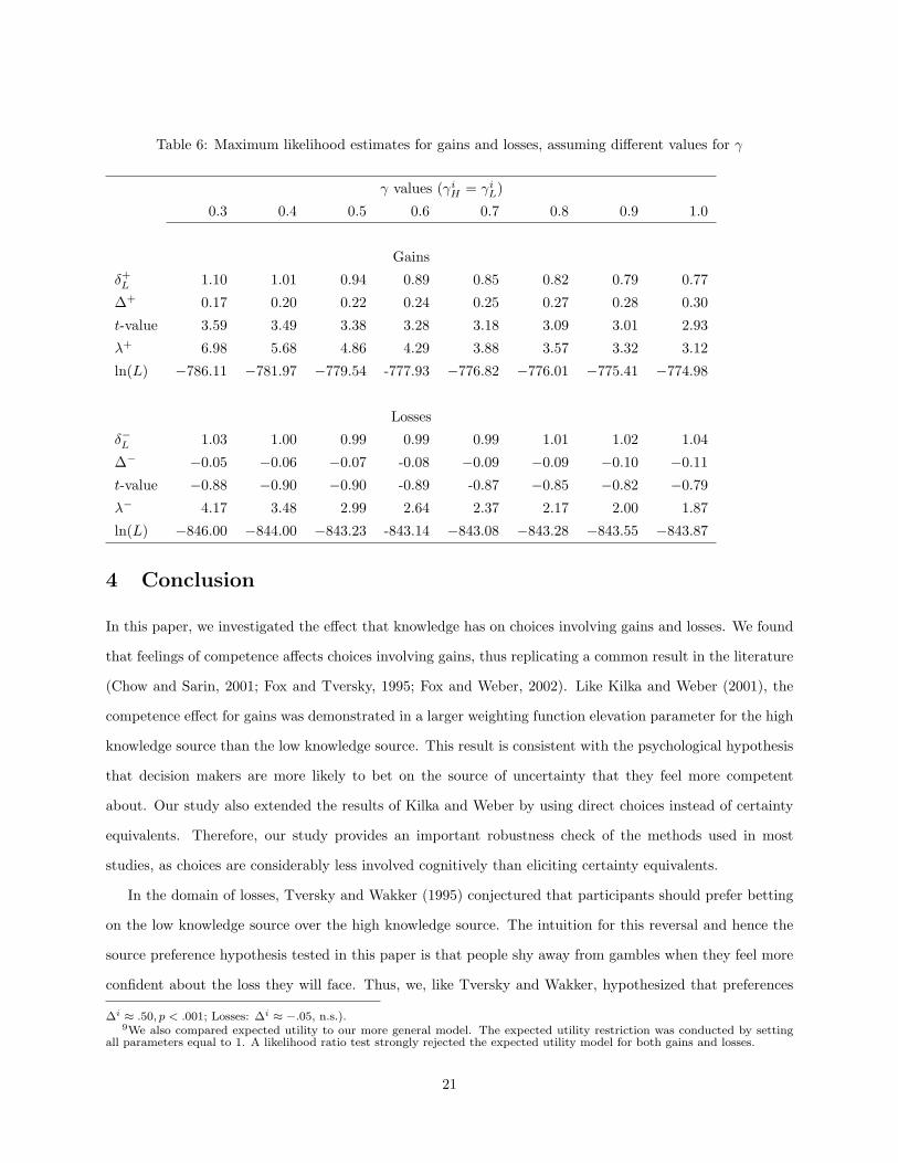
Table 6: Maximum likelihood estimates for gains and losses, assuming different values for γ

γ values (γiH = γiL)

0.3 0.4 0.5 0.6 0.7 0.8 0.9 1.0

Gains

δ+L 1.10 1.01 0.94 0.89 0.85 0.82 0.79 0.77

∆+ 0.17 0.20 0.22 0.24 0.25 0.27 0.28 0.30

t-value 3.59 3.49 3.38 3.28 3.18 3.09 3.01 2.93

λ+ 6.98 5.68 4.86 4.29 3.88 3.57 3.32 3.12

ln(L) −786.11 −781.97 −779.54 -777.93 −776.82 −776.01 −775.41 −774.98

Losses

δ−L 1.03 1.00 0.99 0.99 0.99 1.01 1.02 1.04

∆− −0.05 −0.06 −0.07 -0.08 −0.09 −0.09 −0.10 −0.11

t-value −0.88 −0.90 −0.90 -0.89 -0.87 −0.85 −0.82 −0.79

λ− 4.17 3.48 2.99 2.64 2.37 2.17 2.00 1.87

ln(L) −846.00 −844.00 −843.23 -843.14 −843.08 −843.28 −843.55 −843.87

4 Conclusion

In this paper, we investigated the effect that knowledge has on choices involving gains and losses. We found

that feelings of competence affects choices involving gains, thus replicating a common result in the literature

(Chow and Sarin, 2001; Fox and Tversky, 1995; Fox and Weber, 2002). Like Kilka and Weber (2001), the

competence effect for gains was demonstrated in a larger weighting function elevation parameter for the high

knowledge source than the low knowledge source. This result is consistent with the psychological hypothesis

that decision makers are more likely to bet on the source of uncertainty that they feel more competent

about. Our study also extended the results of Kilka and Weber by using direct choices instead of certainty

equivalents. Therefore, our study provides an important robustness check of the methods used in most

studies, as choices are considerably less involved cognitively than eliciting certainty equivalents.

In the domain of losses, Tversky and Wakker (1995) conjectured that participants should prefer betting

on the low knowledge source over the high knowledge source. The intuition for this reversal and hence the

source preference hypothesis tested in this paper is that people shy away from gambles when they feel more

confident about the loss they will face. Thus, we, like Tversky and Wakker, hypothesized that preferences

∆i ≈ .50, p < .001; Losses: ∆i ≈ −.05, n.s.).9We also compared expected utility to our more general model. The expected utility restriction was conducted by setting

all parameters equal to 1. A likelihood ratio test strongly rejected the expected utility model for both gains and losses.

21

0.0

0.1

0.2

0.3

0.4

0.5

0.6

0.7

0.8

0.9

1.0

0.0 0.1 0.2 0.3 0.4 0.5 0.6 0.7 0.8 0.9 1.0

w(p

)

p

High Knowledge

Low Knowledge

GainsGains

0.0

0.1

0.2

0.3

0.4

0.5

0.6

0.7

0.8

0.9

1.0

0.0 0.1 0.2 0.3 0.4 0.5 0.6 0.7 0.8 0.9 1.0

w(p

)

p

High Knowledge

Low Knowledge

Losses

Figure 3: The decision weighting functions for gains (left panel) and losses (right panel), estimated fromchoices (γiH = γiL = .7).

reflected as they moved from gains to losses. In decision under risk, decision makers are typically risk-averse

for gains and risk-seeking for losses. The focal point for choice changes from gaining with certainty to the

possibility of losing nothing, a crucial psychological distinction between choices in the domain of losses and

choices in the domain of gains that has been observed in previous research on decision under risk.

Interestingly, we found that the hypothesized extension of the competence effect did not extend well to

losses. The hypothesized pattern was significant in only 1 of 6 tests (and marginally significant in another),

and the decision weighting function parameters estimated were not significantly different for less familiar

domains compared to more familiar domains.

We suggest several reasons for the absence of a significant competence effect for losses. First, in Section

2, we reviewed studies of ambiguity aversion for losses. Past studies like Cohen, Jaffray and Said (1985,

see also Einhorn and Hogarth, 1986; Hogarth and Einhorn, 1990; Kahn and Sarin, 1988) show that results

are usually mixed for losses. One reason for this is that choices for losses are noisier. This interpretation is

supported by our estimates of the logit parameter λ, which are lower for losses than gains, indicating that

choosing among losses is noisier than choosing among gains.

Second, by equating the amount to win for each choice gamble, as well as many of the characteristics

of the underlying events, our experimental design provides a stark test of the competence hypothesis. For

example, the events ChiTemp and BuchTemp shared the same target temperature and target day. As a

result, a participant confronted with the choice of whether to select (ChiTemp, x) or (BuchTemp, x) might

22

have simplified the choice to a judgment of whether Chicago or Bucharest was more likely to be 85◦ on

July 15, 2005. Of course, such a simplifying strategy would have produced choices consistent with SEU.

Apparently participants did not resort to such an approach when choosing among gains, but it is possible that

they did so when faced with losses. Such a speculation is consistent with two well-documented observations:

(i) response times are higher for losses than gains (Dickhaut et al, 2003); and (ii) participants are more likely

to use constructive decision processes as task complexity increases (e.g., Bettman, Luce, and Payne, 1998).

If this conjecture is true, then the competence effect for losses may be observed when participants provide

cash equivalents, as in Kilka and Weber (2001), a response mode that is incompatible with the simplifying

strategy outlined above.

Finally, competence may simply not be used to differentiate events when choices involve losses. Indeed,

studies point to neurophysiological differences between reactions to gains and losses (e.g., Samanez-Larkin

et al, 2007). If this is the case, it means that there is a crucial behavioral difference in choices involving

gains from choices involving losses. The psychological reasons for this difference in behavior across the two

domains awaits further investigation.

Acknowledgements

We thank Hugo Sonnenschein and Lars Hansen for their help and Peter Wakker for his useful comments.

Special thanks goes to Heleno Pioner. Jose Guilherme de Lara Resende gratefully acknowledges financial

support from the Coordenacao de Aperfeicoamento de Pessoal de Nıvel Superior (CAPES), Ministry of

Education, Brasil, and from the Haddad fellowship, University of Chicago.

References

[1] Abdellaoui, Mohammed (2000). “Parameter-free elicitation of utility and probability weighting func-tions,” Management Science 46, 1497-1512.

[2] Abdellaoui, Mohammed, Frank Vossmann, and Martin Weber (2005). “Choice-based elicitation anddecomposition of decision weights for gains and losses under uncertainty,” Management Science 51,1384-1399.

[3] Abdellaoui, Mohammed, Han Bleichrodt, and Corina Paraschiv (2007). “Measuring loss aversion: Aparameter-free approach,” Management Science 53, 1659-1674.

[4] Ballinger, T. Parker and Nathaniel T. Wilcox (1997). “Decisions, error and heterogeneity,” EconomicJournal 106, 1090-1105.

23

[5] Baillon, Aurlien, Olivier l’Haridon, and Laetitia Placido (2008), “Risk, Ambiguity, and the Rank-Dependent Axioms: Comments,” working paper.

[6] Basili, Marcello, Alain Chateauneuf, and Fulvio Fontini (2005). “Choices under ambiguity with familiarand unfamiliar outcomes,” Theory and Decision 58, 195-207.

[7] Becker, Selwyn W. and Fred O. Brownson (1964). “What price ambiguity? Or the role of ambiguity indecision-making,” Journal of Political Economy 72, 62-73.

[8] Bettman, James R., Mary F. Luce, and John W. Payne (1998). “Constructive Consumer Choice Pro-cesses.” Journal of Consumer Research 25, 187-217.

[9] Birnbaum, Michael H. and William R. McIntosh (1996). “Violations of branch independence in choicesbetween gambles,” Organizational Behavior and Human Decision Processes 67, 91-110.

[10] Blavatskyy, Pavlo (2007). “Stochastic expected utility theory,” Journal of Risk and Uncertainty 34,259-286.

[11] Brenner, Lyle A. and Yuval Rottenstreich. (1999). “Focus, repacking, and the judgment of groupedhypotheses,” Journal of Behavioral Decision Making 12, 141-148.

[12] Camerer, Colin F. and Teck-Hua Ho (1994). “Violations of the betweenness axiom and nonlinearity inprobability,” Journal of Risk and Uncertainty 8, 167-196.

[13] Camerer, Colin F. and Robin Hogarth (1999). “The effects of financial incentives in experiments: Areview and capital-labor-production framework,” Journal of Risk and Uncertainty 3, 7-42.

[14] Camerer, Colin F. and Martin Weber (1992). “Recent developments in modeling preferences: Uncer-tainty and ambiguity,” Journal of Risk and Uncertainty 5, 325-370.

[15] Choquet, Gustave (1954). “Theory of capacities,” Annales de l’Institut Fourier 5, 131-295.

[16] Chow, Claire Chua and Rakesh K. Sarin (2001). “Comparative ignorance and the Ellsberg paradox,”Journal of Risk and Uncertainty 2, 129-139.

[17] Cohen, Michelle, Jean-Yves Jaffray, and Tanios Said (1985). “Individual behavior under risk and underuncertainty: An experimental study,” Theory and Decision 18, 203-228.

[18] de Bruin, Wandi Bruine, Baruch Fischhoff, Susan G. Millstein, and Bonnie L. Halpern-Felsher (2000).“Verbal and numerical expressions of probability: ‘It’s a fifty-fifty chance’,” Organizational Behaviorand Human Decision Processes 81, 115-131.

[19] Dickhaut, John, Kevin McCabe, Jennifer C. Nagode, Aldo Rustichini, Kip Smith, and Jose V. Pardo(2003). “The impact of the certainty context on the process of choice.” Proceedings of the NationalAcademy of Sciences of the USA 100, 3536-3541.

[20] Einhorn, Hillel J. and Robin M. Hogarth (1986). “Decision making under ambiguity,” Journal of Busi-ness 59, S225-S250.

[21] Ellsberg, Daniel (1961). “Risk, ambiguity and the Savage axioms,” Quarterly Journal of Economics 75,643-669.

[22] Etchart-Vincent, Nathalie (2004). “Is probability weighting sensitive to the magnitude of consequences?An experimental investigation on losses,” Journal of Risk and Uncertainty 3, 217-235.

[23] Fischer, Gregory W., Ziv Carmon, Dan Ariely, and Gal Zauberman (1999). “Goal-based constructionof preferences: Task goals and the prominence effect,” Management Science 45, 1057-1075.

[24] Fox, Craig R. and Amos Tversky (1995). “Ambiguity aversion and comparative ignorance,” QuarterlyJournal of Economics 110, 585-603.

24

[25] Fox, Craig R. and Amos Tversky (1998). “A Belief-based account of decision under uncertainty,” Man-agement Science 44, 879-895.

[26] Fox, Craig R. and Kelly E. See (2003). “Belief and preference in decision under uncertainty,” In D.Hardman and L. Macchi (Eds.), Thinking: Psychological Perspectives on Reasoning, Judgment andDecision Making, New York: Wiley, pp. 273-314.

[27] Fox, Craig R. and Martin Weber (2002). “Ambiguity aversion, comparative ignorance and decisioncontext,” Organizational Behavior and Human Decision Processes 88, 476-498.

[28] Frisch, Deborah and Jonathan Baron (1988). “Ambiguity and rationality,” Journal of Behavioral Deci-sion Making 1, 149-157.

[29] Gilboa, Itzhak (1987). ”Expected utility with purely subjective nonadditive probabilities,” Journal ofMathematical Economics 16, 65-88.

[30] Goldstein, William M. and Hillel J. Einhorn (1987). “Expression theory and the preference reversalphenomena,” Psychological Review 94, 236-254.

[31] Gonzalez, Richard and George Wu (1999). “On the shape of the probability weighting function,” Cog-nitive Psychology 38, 129-166.

[32] Harless, David W. and Colin F. Camerer (1994). “The predictive utility of generalized expected utilitytheories,” Econometrica 62, 1251-1290.

[33] Heath, Chip and Amos Tversky (1991). “Preference and belief: Ambiguity and competence in choiceunder uncertainty,” Journal of Risk and Uncertainty 4, 5-28.

[34] Hertwig, Ralph and Andreas Ortmann (2001). “Experimental practices in economics: A methodologicalchallenge for psychologists?,” Behavioral and Brain Sciences 24, 383403.

[35] Hey, John D. (1995). “Experimental investigations of errors in decision-making under risk,” EuropeanEconomic Review 39, 633-640.

[36] Hogarth, Robin M. and Hillel J. Einhorn (1990). “Venture theory: A model of decision weights,”Management Science 36, 780-803.

[37] Kahn, Barbara E. and Rakesh K. Sarin (1988). “Modelling ambiguity in decisions under uncertainty,”Journal of Consumer Research 15, 265-272.

[38] Kahneman, Daniel and Amos Tversky (1979). “Prospect theory: An analysis of decision under risk,”Econometrica 47, 263-291.

[39] Keynes, John M. (1921). A treatise on probability. London: Macmillan.

[40] Kilka, Michael and Martin Weber (2001). “What determines the shape of the probability weightingfunction under uncertainty?,” Management Science 47, 1712-1726.

[41] Lattimore, Pamela K., Joanna K. Baker, and Ann D. Witte (1992). “The influence of probability onrisky choice: A parametric examination,” Journal of Economic Behavior and Organization 17, 377-400.

[42] Loomes, Graham and Robert Sugden (1998). “Testing Different Stochastic Specifications of RiskyChoice,” Economica 65, 581-598.

[43] Macchi, Laura, Daniel Osherson, and David M. Krantz (1999). “A note on superadditive probabilityjudgment,” Psychological Review 106, 210-214.

[44] Machina, Mark J. (2009). “Risk, ambiguity, and the rank-dependence axioms,” American EconomicReview 99, 385-392.

25

[45] Maxwell, A. E. (1970) “Comparing the classification of subjects by two independent judges,” BritishJournal of Psychiatry 116, 651-655.

[46] Prelec, Drazen (1998). “The probability weighting function,” Econometrica 66, 497-527.

[47] Quiggin, John (1982). “A theory of anticipated utility,” Journal of Economic Behavior and Organization3, 323-343.

[48] Samanez-Larkin, Gregory R., Sasha E. B. Gibbs, Kabir Khanna, Lisbeth Nielsen, Laura L. Carstensen,and Brian Knutson (2007), “Anticipation of monetary gain but not loss in healthy older adults,” NatureNeuroscience 10, 787-791.

[49] Savage, Leonard J. (1954). The Foundations of Statistics. Wiley: New York.

[50] Schmeidler, David (1989). “Subjective probability and expected utility without additivity,” Economet-rica 57, 571-587.

[51] See, Kelly E. (2009). “Reactions to decisions with uncertain consequences: Reliance on perceived fairnessversus predicted outcomes depends on knowledge.” Journal of Personality and Social Psychology 96,104-118.

[52] Stott, Henry (2006). “Cumulative prospect theory’s functional menagerie,” Journal of Risk and Uncer-tainty 32, 101-130.

[53] Stuart, Alan (1955). “A test for homogeneity of the marginal distributions in a two-way classification,”Biometrika 42, 412-416.

[54] Taylor, Kimberly A. (1995). “Testing Credit and Blame Attributions as Explanation for Choices underAmbiguity,” Organizational Behavior & Human Decision Processes 64, 128-137.

[55] Thaler, Richard and Eric Johnson (1990). “Gambling with the House Money and Trying to Break Even:The Effects of Prior Outcomes on Risky Choice,” Management Science 36, 643-660.

[56] Trautmann, Stefan T., Ferdinand M. Vieider, and Peter P. Wakker (2008). “Causes of ambiguity aver-sion: Known versus unknown preferences,” Journal of Risk and Uncertainty 36, 225-243.

[57] Tversky, Amos and Craig R. Fox (1995). “Weighing risk and uncertainty,” Psychological Review 102,269-283.

[58] Tversky, Amos and Daniel Kahneman (1992). “Advances in prospect theory: Cumulative representationof uncertainty,” Journal of Risk and Uncertainty 5, 297-323.

[59] Tversky, Amos and Derek J. Koehler (1994). “Support theory: A nonextensional representation ofsubjective probabilities,” Psychological Review 101, 547-567.

[60] Tversky, Amos and Peter Wakker (1995). “Risk attitudes and decision weights,” Econometrica 63,1255-1280.

[61] Wakker, Peter P. (1990). “Under Stochastic Dominance Choquet-Expected Utility and AnticipatedUtility are Identical,” Theory and Decision 29, 119-132.

[62] Wakker, Peter P. (2004). “On the Composition of Risk Preference and Belief,” Psychological Review111, 236-241.

[63] Wilcox, Nathaniel T. (2008), “Stochastic Models for Binary Discrete Choice under Risk: A CriticalPrimer and Econometric Comparison.” In James C. Cox and Glenn W. Harrison (Eds.), Risk Aversionin Experiments; Research in Experimental Economics, Volume 12, Bingley, UK: Emerald, pp. 197-292.

[64] Wu, George and Richard Gonzalez (1996). “Curvature of the probability weighting function,” Manage-ment Science 42, 1676-1690.

26

[65] Wu, George and Richard Gonzalez (1999). “Nonlinear decision weights in choice under uncertainty,”Management Science 45, 74-85.

[66] Wu, George and Alex B. Markle (2008). “An empirical test of gain-loss separability in prospect theory,”Management Science 54, 1322-1335.

27