Compensation of Loudspeaker Nonlinearities.pdf

Compensation of Loudspeaker Nonlinearities

- DSP implementation.

1th July 2007.

Karsten Øyen

Master Thesis

Ørsted·DTU – Acoustic Technology Technical University of Denmark

2

Contents Contents .......................................................................................................................................... 1 Preface ............................................................................................................................................. 5 Notation ........................................................................................................................................... 7 Summary.......................................................................................................................................... 9 Introduction ................................................................................................................................... 10

1.1 The Concept of the Adaptive Controller ................................................................................ 11 1.2 Specifications for the project ................................................................................................. 12

2. The Loudspeaker – a short introduction. ............................................................................ 13 2.1 The History ............................................................................................................................ 13 2.2 The principle.......................................................................................................................... 13 2.3 The loudspeaker behaviour due to the resonance frequency. .............................................. 14 2.4 Acoustical Power Radiation................................................................................................... 14 2.5 Generally About Loudspeaker Modelling .............................................................................. 14

3. Linear Modelling .................................................................................................................... 15 3.1 Electrical, Mechanical and Acoustical Analogous Circuits. ................................................... 15

3.1.1 Electrical System ............................................................................................................ 15 3.1.2 Mechanical System......................................................................................................... 16 3.1.3 Acoustical System .......................................................................................................... 16

3.2 The State Space Model - linear............................................................................................. 17 3.2.1 Forward Euler ................................................................................................................. 17 3.2.2 Conversion of the analogous equations to digital, discrete domain................................ 17 3.2.3 Predicting the next state value of the Voice-coil Current, )1( +niLe ............................... 17 3.2.4 Predicting next state value of the diaphragm Velocity, )1( +nv ..................................... 18 3.2.5 Predicting the diaphragm Position, )1( +nx ................................................................... 18 3.2.6 The Final Matrix of The State Space Model - linear ....................................................... 18

3.3 Extension of the linear model. – including eddy currents. ..................................................... 19 4. Loudspeaker Nonlinearities..................................................................................................... 20

4.1 Position Dependent Parameters ........................................................................................... 21 4.1.1 The Position Dependent Force Factor............................................................................ 21 4.1.2 The Position Dependent Suspension ............................................................................. 21 4.1.3 The Position Dependent Inductance............................................................................... 22

4.2 Other Nonlinearities............................................................................................................... 22 4.2.1 Compliance creep........................................................................................................... 22 4.2.2 The Current Dependent Inductance ............................................................................... 22

4.3 Measuring Nonlinear Distortion (THD / IMD)......................................................................... 23 4.3.1 Harmonic distortion......................................................................................................... 23 4.3.2 Intermodulation distortion ............................................................................................... 23

5. Nonlinear Modelling .............................................................................................................. 24 5.1 Electrical, Mechanical and acoustical analogous Circuits. .................................................... 24 5.2 The State Space Model......................................................................................................... 25

5.2.1 The Final Matrix of the State Space Model..................................................................... 25 6. Loudspeaker Parameter Drifting .......................................................................................... 26

6.1 Temperature Drifting.......................................................................................................... 26 6.2 The Drifting of the Compliance .......................................................................................... 26 6.3 Updating the Loudspeaker Model - Due to Parameter Drifting.......................................... 27

7 Compensation of nonlinearities. .......................................................................................... 28 7.1 The Negative Feedback System ........................................................................................... 28

3

7.7.1 Different proposals for measuring the output of the loudspeaker: .................................. 28 7.2 The Feedforward System. ..................................................................................................... 29 7.3 The Adaptive Feedforward System. ...................................................................................... 30 7.4 The Chosen Compensation Algorithm. ................................................................................. 30

7.4.1 Schematic diagram ......................................................................................................... 30 7.4.2 Compensator algorithm .................................................................................................. 32 7.4.3 Modified Compensator algorithm - Including eddy-currents ........................................... 33

8. Loudspeaker - Measurements ......................................................................................... 34 8.1 Loudspeaker Parameters Measurement ......................................................................... 34

8.1.1 The Klippel Analyser....................................................................................................... 34 8.1.2 The Result of Measurement 1. ....................................................................................... 35 8.1.3 The Results of Measurement 2 – updated software. ...................................................... 37 8.1.4 Comparing the Results of Measurement 1 and 2 ........................................................... 38 8.1.5 Linear Parameters – Measurement. ............................................................................... 39

8.2 Nonlinear Parameters Drifting – Measurement. .................................................................... 40 8.3 Loudspeaker Output Measurement – Displacement. ...................................................... 41

9. Matlab simulation...................................................................................................................... 42 9.1 Overview of Matlab functions .......................................................................................... 42 9.2 The Modelling of the Nonlinear Parameter............................................................................ 43 9.2.1 Stretching / Scaling of the compliance ............................................................................... 43 9.3 The Loudspeaker Model........................................................................................................ 44

9.3.1 Simulation in Matlab - Compared to Loudspeaker Measurement................................... 44 9.3.2 Model with Compliance Adjustment.- Compared to Real Loudspeaker. ........................ 46

9.4 The Nonlinear Compensator ........................................................................................... 48 9.4.1 Simulation Result 1......................................................................................................... 48 THD and IMD calculations - of the Simulated Power Radiation. ............................................. 49 9.3.2 Simulation Result 2......................................................................................................... 49 9.3.3 Simulation Result 3 – Eddy-current in both model and compensator ............................. 49 9.3.3 Simulation Result 3 – Eddy-current in both model and compensator ............................. 50 9.3.4 Comments of the simulation. .......................................................................................... 50 9.3.5 Instability problem with the compensation algorithm ...................................................... 51

10. DSP Programming .................................................................................................................. 51 10.1 Overview of DSP functions.................................................................................................. 51 10.2 Development kit/Software. .................................................................................................. 52 10.3 The nonlinear compensation - Simulation. .......................................................................... 53

10.3.1 Implementation of Tables. ............................................................................................ 53 10.4 Comparing DSP Simulation and Matlab Simulation ........................................................ 57

11 The final Measurement. .................................................................................................... 58 11.1 Schematic Drawing ............................................................................................................. 58 11.2 Description of the Setup ...................................................................................................... 58 11.3 Measurement result............................................................................................................. 60

11.3 Measurement result 1. ..................................................................................................... 61 11.3 Measurement result 2 – with adjustment of the compliance curve. ................................. 63 -................................................................................................................................................ 64

11.4 Discussion ........................................................................................................................... 64 12. The Future Setup............................................................................................................... 66

12.1 Schematic Drawing – The adaptive system ........................................................................ 66 12.2 Description .......................................................................................................................... 66

Hardware ................................................................................................................................. 66 Software Blocks ....................................................................................................................... 66 Analog signals ......................................................................................................................... 67 Discrete, digital signals ............................................................................................................ 67 Others symbols........................................................................................................................ 67

4

Description of the Setup .......................................................................................................... 67 12.3. Proposal for Voltage/current measurement........................................................................ 68

13. Conclusion......................................................................................................................... 69 14. References......................................................................................................................... 70 Appendix A Matlab Code.............................................................................................................. 71

A1. linear_Loudspeaker_Model_Simplified ................................................................................. 71 A2.Loudspeaker_Model_Simplified............................................................................................. 72 A3. Loudspeaker_Model ............................................................................................................. 73 A4. Nonlinear_Compensator_Simplified ..................................................................................... 74 A5. Nonlinear_Compensator ....................................................................................................... 76 A6 compliance_Adjustment......................................................................................................... 78 A7 THD........................................................................................................................................ 79 A8 IMD ........................................................................................................................................ 80 A9 Load_Nonlinear_Parameters ................................................................................................. 81 A10 Load_Linear_Parameter ...................................................................................................... 82 A11 plot_Nonlinearparameter ..................................................................................................... 83 A12 Capture ................................................................................................................................ 85 A13 Main ..................................................................................................................................... 86

Appendix B - C-Code .................................................................................................................... 88 B1 linear_model .......................................................................................................................... 88 B2 nonlinear_model .................................................................................................................... 89 A3. nonlinear_model_comp......................................................................................................... 91 B4 get_linear_parameters ........................................................................................................... 92 B6 Gain ....................................................................................................................................... 93 B7 Peak....................................................................................................................................... 94 B8 Rms........................................................................................................................................ 94 B8 add_matrices_3 ..................................................................................................................... 94 B9 mult_matrices_3..................................................................................................................... 94 B10 add_matrices_4 ................................................................................................................... 95 B11 mult_matrices_4................................................................................................................... 95 B12 main ..................................................................................................................................... 96

5

Preface This master thesis is carried out in corporation with Bang & Olufsen, located in Struer. In all eight weeks are spent at Bang & Olufsen in Struer, and the rest at Ørsted DTU – The Technical University of Denmark. I would like to thank Finn Agerkvist, my supervisor at DTU, and I would like to thank Sylvain Choisel, Søren Beck and Gert Munch, and the acoustical apartment in Struer, for great helping and great inspiration. Karsten Øyen, 1th July 2007, Cohenhaven

6

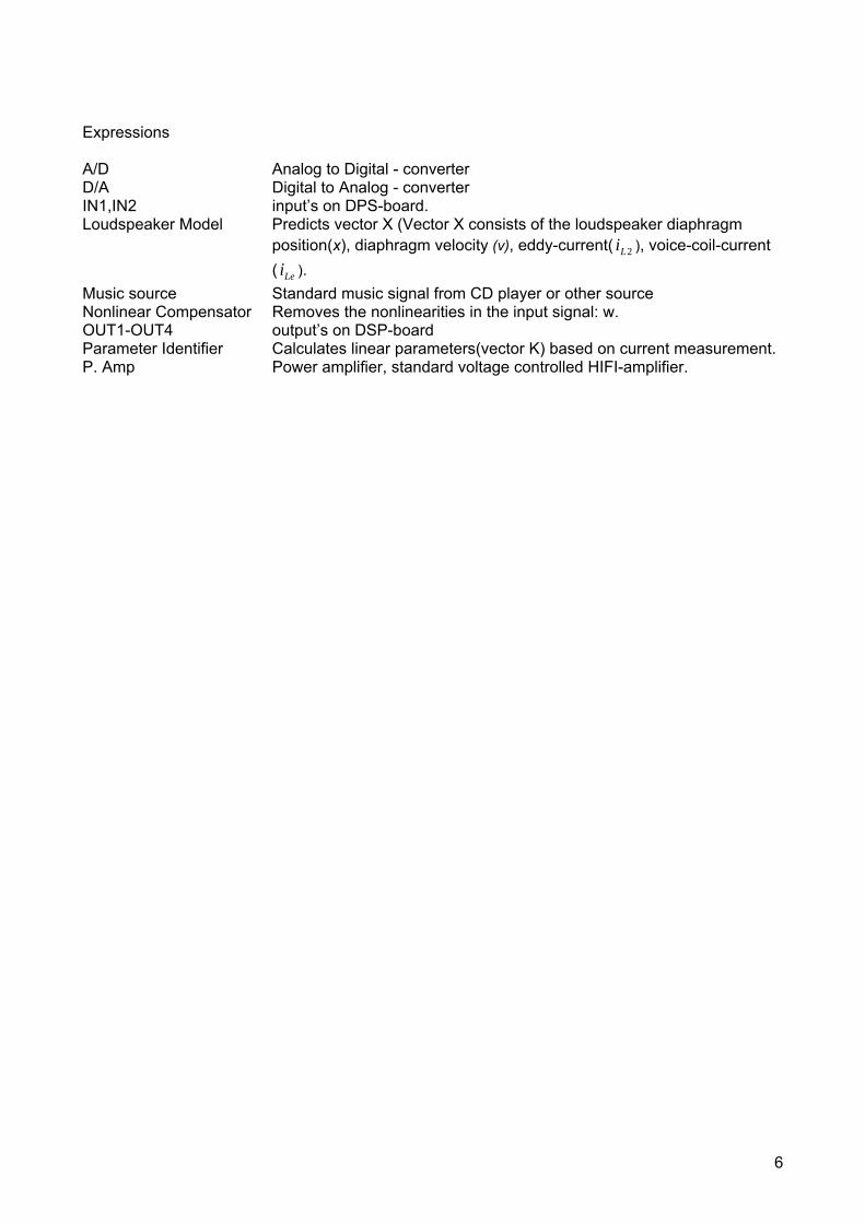
Expressions A/D Analog to Digital - converter D/A Digital to Analog - converter IN1,IN2 input’s on DPS-board. Loudspeaker Model Predicts vector X (Vector X consists of the loudspeaker diaphragm

position(x), diaphragm velocity (v), eddy-current( 2Li ), voice-coil-current ( Lei ).

Music source Standard music signal from CD player or other source Nonlinear Compensator Removes the nonlinearities in the input signal: w. OUT1-OUT4 output’s on DSP-board Parameter Identifier Calculates linear parameters(vector K) based on current measurement. P. Amp Power amplifier, standard voltage controlled HIFI-amplifier.

7

Notation Symbol Deskription Unit a Loudspeaker diaphragm acceleration. [m/ 2s ] B: Magnetic field. Bl Force factor, the product of B(magnet field) and l(effective length of voice-coil). [N/A]

0Bl Force factor, at x=0. [N/A] C_str Factor for tuning the compliance curve, stretches the x-axe curve. C_sca Factor for tuning the compliance curve, scales the curve

tC : Mechanical compliance of driver suspension [m/N]

0C : Mechanical compliance of driver suspension, at x=0. [m/N] Fs: Loudspeaker resonance frequency [Hz] F(n): Matrix used in state space model G(n): Matrix used in state space model

Lei : Voice-coil current. [A]

mLei Voice-coil current – measured value. [A]

2Li Voice-coil eddy-current, induced by the loudspeaker [A] G Power Amplifier Gain. k: Mechanical stiffness of driver suspension(1/C ) N/m]

0k : Mechanical stiffness of driver suspension, at x=0. (1/ 0C ) N/m] K(n) Vector consisting of linear parameter l: Effective length of the voice-coil. [m]

2L : Para-inductance of voice coil, due to eddy current losses. [H]

eL : Voice coil inductance. [H]

0eL : Voice coil inductance, at x=0. [H]

eL : Frequency independent part of Voice coil inductance. [H]

tM : Mechanical mass of driver diaphragm, air load and voice-coil. [kg]

DP Pressure difference between the rear and the front of the loudspeaker diaphragm. [Pa]

ARP Power Radiation [Pa]

tR Mechanical resistance of total-driver losses [kg/s]

2R : Electrical resistance, due to eddy current losses. [Ω]

eR : Electrical voice coil resistance at DC. [Ω]

Rs: Shunt resistor for measuring voice-coil current: Lei [Ω] Ra-Rd: Feedback network for loudspeaker current -and voltage measurement. [Ω]

DSPinR Input resistance for analogous inputs on DSP board. [Ω]

DS : The area of the diaphragm. [ 2m ] Ts: 1/samplingfrequency [s] u (n): Processed input signal for loudspeaker, digital, discrete. [V]

)(tuD Driver voltage. Amplified, music signal applied to the loudspeaker. [V] u (n)’: Feedback measurement of u(t). [V] u (t): Processed music signal, analogous signal. [V] U Loudspeaker diaphragm volume velocity. [ 2m /s] v : Loudspeaker diaphragm velocity [m/s] w(n): Signal from music source, digital, discrete. [V]

8

w(t): Signal from music source, analog signal. [V] x (n): Loudspeaker diaphragm position [m] X(n): Predicted state vector (one sample into the future). Consists of current, Lei ,

eddy current, 2Li , voice-coil position x (n) - and velocity, )(nv .

resZ Loudspeaker impedance at the resonance frequency [Ω]

ARZ Acoustical impedance at the back side of the loudspeaker diaphragm [Pa]

AFZ Acoustical impedance in the front of the loudspeaker diaphragm [Pa]

xLe

∂∂ : First derivate of eL with respect to position ( )(nx ). [H/m]

xL∂∂ 2 : First derivate of 2L with respect to position - )(nx . [H/m]

9

Summary Compensation of loudspeaker nonlinearities is investigated. A feedforward compensation system, based a loudspeaker model (a computer simulation of the real loudspeaker), is first simulated in matlab and later implemented on DSP. The system is briefly tested for pure tones with and the loudspeaker diaphragm excursion is used as output measure. To carry out an adaptive system, able to handle the loudspeaker drifting due to temperature and aging, is a subject for further investigation. An adaptive system using current measurement for feedback is in mind. A future setup is to a certain degree described. Without the adaptive part, the compensation system is briefly tested in a simplified setup. The loudspeaker model is manually adjusted to fit the real loudspeaker. The compliance of the suspension is tuned in realtime by stretching and scaling functionality implemented on DSP. The system seems to work for some input frequencies and do not work for others.

10

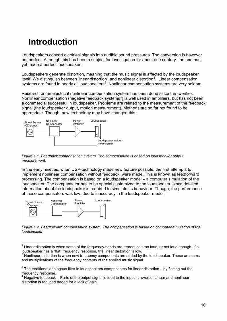
Introduction Loudspeakers convert electrical signals into audible sound pressures. The conversion is however not perfect. Although this has been a subject for investigation for about one century - no one has yet made a perfect loudspeaker. Loudspeakers generate distortion, meaning that the music signal is affected by the loudspeaker itself. We distinguish between linear distortion1 and nonlinear distortion2. Linear compensation systems are found in nearly all loudspeakers3. Nonlinear compensation systems are very seldom. Research on an electrical nonlinear compensation system has been done since the twenties. Nonlinear compensation (negative feedback systems4) is well used in amplifiers, but has not been a commercial successful in loudspeaker. Problems are related to the measurement of the feedback signal (the loudspeaker output, motion measurement). Methods are so far not found to be appropriate. Though, new technology may have changed this. Figure 1.1. Feedback compensation system. The compensation is based on loudspeaker output measurement. In the early nineties, when DSP-technology made new feature possible, the first attempts to implement nonlinear compensation without feedback, were made. This is known as feedforward processing. The compensation is based on a loudspeaker model – a computer simulation of the loudspeaker. The compensator has to be special customized to the loudspeaker, since detailed information about the loudspeaker is required to simulate its behaviour. Though, the performance of these compensators was low, due to inaccuracy in the loudspeaker model, Figure 1.2. Feedforward compensation system. The compensation is based on computer-simulation of the loudspeaker. 1 Linear distortion is when some of the frequency-bands are reproduced too loud, or not loud enough. If a loudspeaker has a “flat” frequency response, the linear distortion is low. 2 Nonlinear distortion is when new frequency components are added by the loudspeaker. These are sums and multiplications of the frequency contents of the applied music signal. 3 The traditional analogous filter in loudspeakers compensates for linear distortion – by flatting out the frequency response. 4 Negative feedback - Parts of the output signal is feed to the input in reverse. Linear and nonlinear distortion is reduced traded for a lack of gain.

Signal Source (CD-player)

Nonlinear Compensator

Power Amplifier

Loudspeaker

Loudspeaker output -measurement



Power Amplifier

Loudspeaker

11

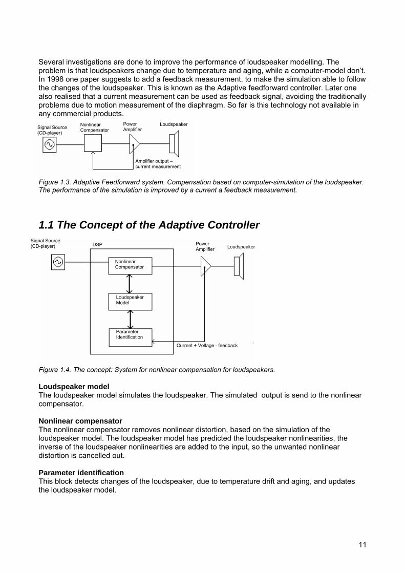
Several investigations are done to improve the performance of loudspeaker modelling. The problem is that loudspeakers change due to temperature and aging, while a computer-model don’t. In 1998 one paper suggests to add a feedback measurement, to make the simulation able to follow the changes of the loudspeaker. This is known as the Adaptive feedforward controller. Later one also realised that a current measurement can be used as feedback signal, avoiding the traditionally problems due to motion measurement of the diaphragm. So far is this technology not available in any commercial products.

Figure 1.3. Adaptive Feedforward system. Compensation based on computer-simulation of the loudspeaker. The performance of the simulation is improved by a current a feedback measurement.

1.1 The Concept of the Adaptive Controller

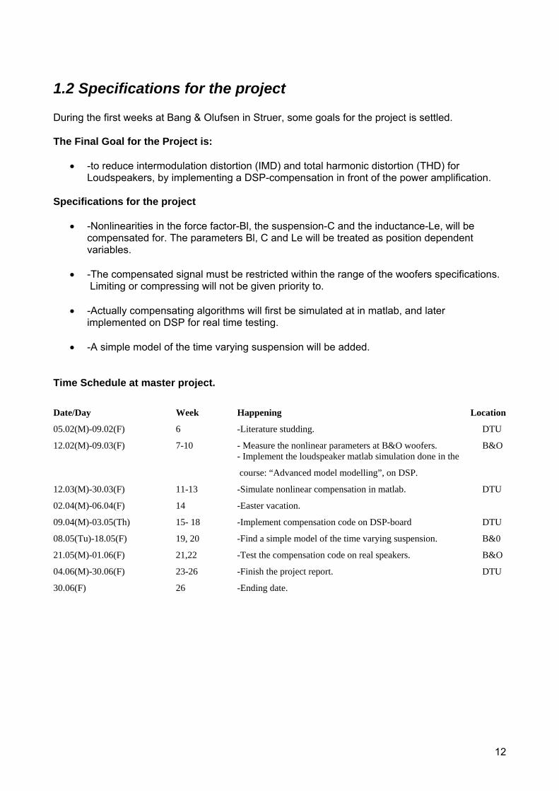
Figure 1.4. The concept: System for nonlinear compensation for loudspeakers. Loudspeaker model The loudspeaker model simulates the loudspeaker. The simulated output is send to the nonlinear compensator. Nonlinear compensator The nonlinear compensator removes nonlinear distortion, based on the simulation of the loudspeaker model. The loudspeaker model has predicted the loudspeaker nonlinearities, the inverse of the loudspeaker nonlinearities are added to the input, so the unwanted nonlinear distortion is cancelled out. Parameter identification This block detects changes of the loudspeaker, due to temperature drift and aging, and updates the loudspeaker model.



Power Amplifier

Loudspeaker

Amplifier output –current measurement

Signal Source (CD-player) Power

Amplifier Loudspeaker DSP


Loudspeaker Model

Parameter Identification

Current + Voltage - feedback

12

1.2 Specifications for the project During the first weeks at Bang & Olufsen in Struer, some goals for the project is settled. The Final Goal for the Project is:

• -to reduce intermodulation distortion (IMD) and total harmonic distortion (THD) for Loudspeakers, by implementing a DSP-compensation in front of the power amplification.

Specifications for the project

• -Nonlinearities in the force factor-Bl, the suspension-C and the inductance-Le, will be compensated for. The parameters Bl, C and Le will be treated as position dependent variables.

• -The compensated signal must be restricted within the range of the woofers specifications. Limiting or compressing will not be given priority to.

• -Actually compensating algorithms will first be simulated at in matlab, and later implemented on DSP for real time testing.

• -A simple model of the time varying suspension will be added.

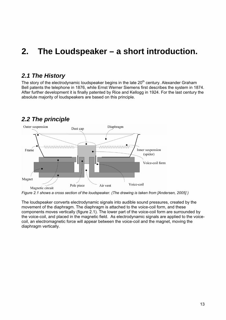
Time Schedule at master project. Date/Day Week Happening Location

05.02(M)-09.02(F) 6 -Literature studding. DTU

12.02(M)-09.03(F) 7-10 - Measure the nonlinear parameters at B&O woofers. B&O - Implement the loudspeaker matlab simulation done in the

course: “Advanced model modelling”, on DSP.

12.03(M)-30.03(F) 11-13 -Simulate nonlinear compensation in matlab. DTU

02.04(M)-06.04(F) 14 -Easter vacation.

09.04(M)-03.05(Th) 15- 18 -Implement compensation code on DSP-board DTU

08.05(Tu)-18.05(F) 19, 20 -Find a simple model of the time varying suspension. B&0

21.05(M)-01.06(F) 21,22 -Test the compensation code on real speakers. B&O

04.06(M)-30.06(F) 23-26 -Finish the project report. DTU

30.06(F) 26 -Ending date.

13

2. The Loudspeaker – a short introduction.

2.1 The History The story of the electrodynamic loudspeaker begins in the late 20th century. Alexander Graham Bell patents the telephone in 1876, while Ernst Werner Siemens first describes the system in 1874. After further development it is finally patented by Rice and Kellogg in 1924. For the last century the absolute majority of loudspeakers are based on this principle.

2.2 The principle

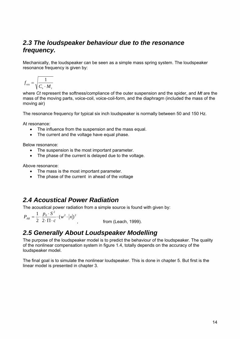
Figure 2.1 shows a cross section of the loudspeaker. (The drawing is taken from [Andersen, 2005] ) The loudspeaker converts electrodynamic signals into audible sound pressures, created by the movement of the diaphragm. The diaphragm is attached to the voice-coil form, and these components moves vertically (figure 2.1). The lower part of the voice-coil form are surrounded by the voice-coil, and placed in the magnetic field. As electrodynamic signals are applied to the voice-coil, an electromagnetic force will appear between the voice-coil and the magnet, moving the diaphragm vertically.

14

2.3 The loudspeaker behaviour due to the resonance frequency. Mechanically, the loudspeaker can be seen as a simple mass spring system. The loudspeaker resonance frequency is given by:

ttres MC

f⋅

=⋅

1

where Ct represent the softness/compliance of the outer suspension and the spider, and Mt are the mass of the moving parts, voice-coil, voice-coil-form, and the diaphragm (included the mass of the moving air) The resonance frequency for typical six inch loudspeaker is normally between 50 and 150 Hz. At resonance:

• The influence from the suspension and the mass equal. • The current and the voltage have equal phase.

Below resonance: • The suspension is the most important parameter. • The phase of the current is delayed due to the voltage.

Above resonance:

• The mass is the most important parameter. • The phase of the current in ahead of the voltage

2.4 Acoustical Power Radiation The acoustical power radiation from a simple source is found with given by:

222

0 )(22

1 xwc

SpPAR ⋅⋅

⋅Π⋅⋅

⋅=, from (Leach, 1999).

2.5 Generally About Loudspeaker Modelling The purpose of the loudspeaker model is to predict the behaviour of the loudspeaker. The quality of the nonlinear compensation system in figure 1.4, totally depends on the accuracy of the loudspeaker model. The final goal is to simulate the nonlinear loudspeaker. This is done in chapter 5. But first is the linear model is presented in chapter 3.

15

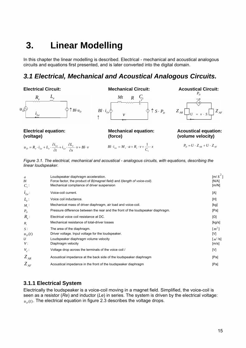
3. Linear Modelling In this chapter the linear modelling is described. Electrical - mechanical and acoustical analogous circuits and equations first presented, and is later converted into the digital domain.

3.1 Electrical, Mechanical and Acoustical Analogous Circuits. Electrical Circuit: Mechanical Circuit: Acoustical Circuit: Electrical equation: Mechanical equation: Acoustical equation: (voltage) (force) (volume velocity)

Figure 3.1. The electrical, mechanical and acoustical - analogous circuits, with equations, describing the linear loudspeaker. a Loudspeaker diaphragm acceleration. [m/

2s ] Bl Force factor, the product of B(magnet field) and l(length of voice-coil). [N/A]








S : The area of the diaphragm. [ 2m ] )(tuD Driver voltage. Input voltage for the loudspeaker. [V]

U Loudspeaker diaphragm volume velocity [ 2m /s] v : Diaphragm velocity [m/s]

cv : Voltage drop across the terminals of the voice coil / [V]



3.1.1 Electrical System Electrically the loudspeaker is a voice-coil moving in a magnet field. Simplified, the voice-coil is seen as a resistor (Re) and inductor (Le) in series. The system is driven by the electrical voltage:

)(tuD . The electrical equation in figure 2.3 describes the voltage drops.

ABZ

eR eL

DuDuBl⋅↑

Lei←

vBlvx

Li

ti

LiRu eLe

LeeLeeD ⋅+⋅

∂∂⋅+

∂∂⋅+⋅= x

CvRaMiBl

tttLe ⋅+⋅+⋅=⋅

1

Mt sR

LeiBl ⋅↑

DPS ⋅↑

tC

v ←

AFABD ZUZUP ⋅+⋅=

SvU ⋅=←

AFZ

DP →

ARZ

16

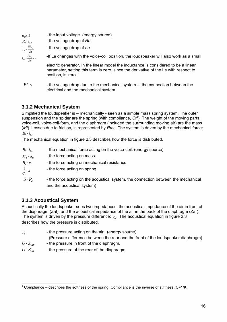
)(tuD - the input voltage. (energy source)

Lee iR ⋅ - the voltage drop of Re.

ti

L Lee ∂

∂⋅ - the voltage drop of Le.

vx

Li e

Le ⋅∂

∂⋅ -If Le changes with the voice-coil position, the loudspeaker will also work as a small

electric generator. In the linear model the inductance is considered to be a linear parameter, setting this term is zero, since the derivative of the Le with respect to position, is zero.

vBl ⋅ - the voltage drop due to the mechanical system – the connection between the

electrical and the mechanical system.

3.1.2 Mechanical System Simplified the loudspeaker is – mechanically - seen as a simple mass spring system. The outer suspension and the spider are the spring (with compliance, Ct5). The weight of the moving parts, voice-coil, voice-coil-form, and the diaphragm (included the surrounding moving air) are the mass (Mt). Losses due to friction, is represented by Rms. The system is driven by the mechanical force:

LeiBl ⋅ The mechanical equation in figure 2.3 describes how the force is distributed.

LeiBl ⋅ - the mechanical force acting on the voice-coil. (energy source)

Dt aM ⋅ - the force acting on mass. vRt ⋅ - the force acting on mechanical resistance.

xCt

⋅1 - the force acting on spring.

dPS ⋅ - the force acting on the acoustical system, the connection between the mechanical and the acoustical system)

3.1.3 Acoustical System Acoustically the loudspeaker sees two impedances, the acoustical impedance of the air in front of the diaphragm (Zaf), and the acoustical impedance of the air in the back of the diaphragm (Zar). The system is driven by the pressure difference:

DP . The acoustical equation in figure 2.3 describes how the pressure is distributed.

DP - the pressure acting on the air, (energy source) (Pressure difference between the rear and the front of the loudspeaker diaphragm)

AFZU ⋅ - the pressure in front of the diaphragm.

ARZU ⋅ - the pressure at the rear of the diaphragm.

5 Compliance – describes the softness of the spring. Compliance is the inverse of stiffness. C=1/K.

17

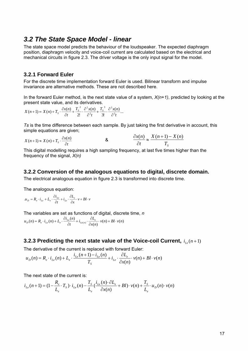
3.2 The State Space Model - linear The state space model predicts the behaviour of the loudspeaker. The expected diaphragm position, diaphragm velocity and voice-coil current are calculated based on the electrical and mechanical circuits in figure 2.3. The driver voltage is the only input signal for the model.

3.2.1 Forward Euler For the discrete time implementation forward Euler is used. Bilinear transform and impulse invariance are alternative methods. These are not described here. In the forward Euler method, is the next state value of a system, X(n+1), predicted by looking at the present state value, and its derivatives.

...)(!3

)(!2

)()()1( 3

33

2

22

tnxT

tnxT

tnxTnXnX SS

S ∂∂⋅+

∂∂⋅+

∂∂⋅+=+

Ts is the time difference between each sample. By just taking the first derivative in account, this simple equations are given;

tnxTnXnX S ∂

∂⋅+≈+

)()()1( & ST

nXnXtnx )()1()( −+

≈∂

∂

This digital modelling requires a high sampling frequency, at last five times higher than the frequency of the signal, X(n)

3.2.2 Conversion of the analogous equations to digital, discrete domain. The electrical analogous equation in figure 2.3 is transformed into discrete time. The analogous equation:

The variables are set as functions of digital, discrete time, n

)()()(

)()()( )( nvBlnvnx

LitniLniRnu e

nLeLe

eLeeD ⋅+⋅∂∂

⋅+∂

∂⋅+⋅=

3.2.3 Predicting the next state value of the Voice-coil Current, )1( +niLe The derivative of the current is replaced with forward Euler: )()(

)()()1()()( nvBlnv

nxLi

TniniLniRnu e

LeS

LeLeeLeeD ⋅+⋅

∂∂

⋅+−+

⋅+⋅=

The next state of the current is:

)()()())(

)(()()1()1( nvnuLTnvBl

nxLni

LTniT

LRni D

e

SeLe

e

SLeS

e

eLe ⋅⋅+⋅+

∂∂⋅

−⋅⋅−=+

vBlvx

Li

ti

LiRu eLe

LeeLeeD ⋅+⋅

∂∂⋅+

∂∂⋅+⋅=.

18

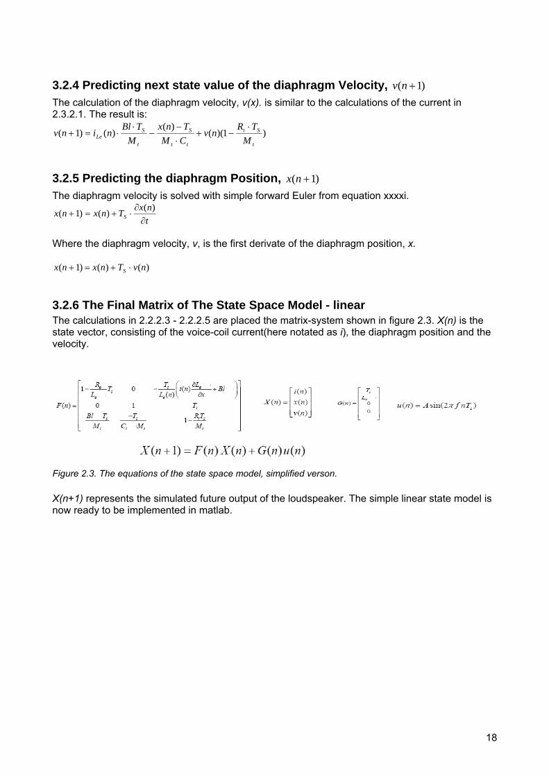
3.2.4 Predicting next state value of the diaphragm Velocity, )1( +nv The calculation of the diaphragm velocity, v(x). is similar to the calculations of the current in 2.3.2.1. The result is:

)1)(()(

)()1(t

St

tt

S

t

SLe M

TRnv

CMTnx

MTBl

ninv⋅

−+⋅−

−⋅

⋅=+

3.2.5 Predicting the diaphragm Position, )1( +nx The diaphragm velocity is solved with simple forward Euler from equation xxxxi.

tnxTnxnx S ∂

∂⋅+=+

)()()1(

Where the diaphragm velocity, v, is the first derivate of the diaphragm position, x.

)()()1( nvTnxnx S ⋅+=+

3.2.6 The Final Matrix of The State Space Model - linear The calculations in 2.2.2.3 - 2.2.2.5 are placed the matrix-system shown in figure 2.3. X(n) is the state vector, consisting of the voice-coil current(here notated as i), the diaphragm position and the velocity.

Figure 2.3. The equations of the state space model, simplified verson. X(n+1) represents the simulated future output of the loudspeaker. The simple linear state model is now ready to be implemented in matlab.

19

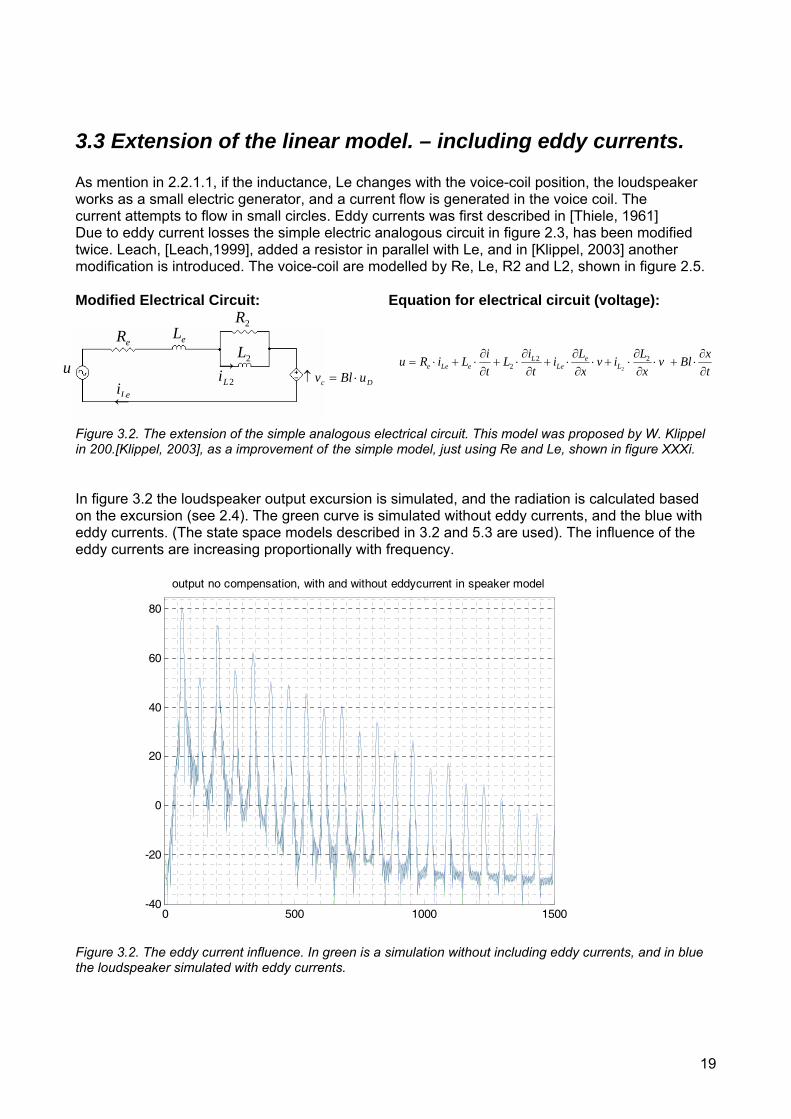
3.3 Extension of the linear model. – including eddy currents. As mention in 2.2.1.1, if the inductance, Le changes with the voice-coil position, the loudspeaker works as a small electric generator, and a current flow is generated in the voice coil. The current attempts to flow in small circles. Eddy currents was first described in [Thiele, 1961] Due to eddy current losses the simple electric analogous circuit in figure 2.3, has been modified twice. Leach, [Leach,1999], added a resistor in parallel with Le, and in [Klippel, 2003] another modification is introduced. The voice-coil are modelled by Re, Le, R2 and L2, shown in figure 2.5. Modified Electrical Circuit: Equation for electrical circuit (voltage):

Figure 3.2. The extension of the simple analogous electrical circuit. This model was proposed by W. Klippel in 200.[Klippel, 2003], as a improvement of the simple model, just using Re and Le, shown in figure XXXi. In figure 3.2 the loudspeaker output excursion is simulated, and the radiation is calculated based on the excursion (see 2.4). The green curve is simulated without eddy currents, and the blue with eddy currents. (The state space models described in 3.2 and 5.3 are used). The influence of the eddy currents are increasing proportionally with frequency.

Figure 3.2. The eddy current influence. In green is a simulation without including eddy currents, and in blue the loudspeaker simulated with eddy currents.

← txBlv

xLiv

xLi

tiL

tiLiRu L

eLe

LeLee ∂

∂⋅+⋅

∂∂⋅+⋅

∂∂⋅+

∂∂⋅+

∂∂⋅+⋅= 22

2 2

eR eL 2R

Dc uBlv ⋅=↑2Li

→ 2L u

Lei ←

0 500 1000 1500-40

-20

0

20

40

60

80

output no compensation, with and without eddycurrent in speaker model

20

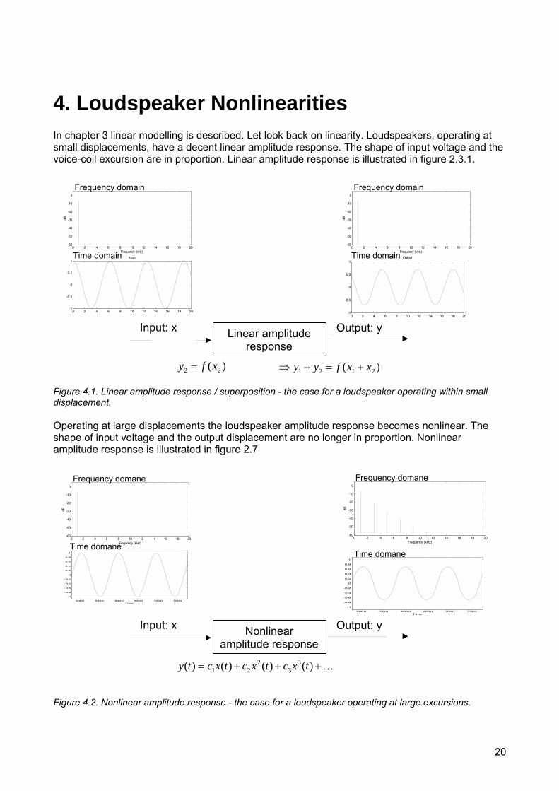
4. Loudspeaker Nonlinearities In chapter 3 linear modelling is described. Let look back on linearity. Loudspeakers, operating at small displacements, have a decent linear amplitude response. The shape of input voltage and the voice-coil excursion are in proportion. Linear amplitude response is illustrated in figure 2.3.1.

)()(

22

11

xfyxfy

==

)( 2121 xxfyy +=+⇒ Figure 4.1. Linear amplitude response / superposition - the case for a loudspeaker operating within small displacement. Operating at large displacements the loudspeaker amplitude response becomes nonlinear. The shape of input voltage and the output displacement are no longer in proportion. Nonlinear amplitude response is illustrated in figure 2.7

K+++= )()()()( 33

221 txctxctxcty

Figure 4.2. Nonlinear amplitude response - the case for a loudspeaker operating at large excursions.

Nonlinear amplitude response

Input: x Output: y

5000 5500 6000 6500 7000 7500

-1

-0.8

-0.6

-0.4

-0.2

0

0.2

0.4

0.6

0.8

1

Time

Time domane Time domane

5000 5500 6000 6500 7000 7500

-1

-0.8

-0.6

-0.4

-0.2

0

0.2

0.4

0.6

0.8

1

Time

0 2 4 6 8 10 12 14 16 18 20-60

-50

-40

-30

-20

-10

0

Frequency [kHz]

dB

Frequency domane

0 2 4 6 8 10 12 14 16 18 20-60

-50

-40

-30

-20

-10

0

Frequency [kHz]

dB

Frequency domane

Linear amplitude response

Input: x Output: y 0 2 4 6 8 10 12 14 16 18 20

-1

-0.5

0

0.5

1OutputTime domain Time domain

0 2 4 6 8 10 12 14 16 18 20-1

-0.5

0

0.5

1Input

0 2 4 6 8 10 12 14 16 18 20-60

-50

-40

-30

-20

-10

0

Frequency [kHz]

dB

Frequency domain

0 2 4 6 8 10 12 14 16 18 20-60

-50

-40

-30

-20

-10

0

Frequency [kHz]

dB

Frequency domain

21

The reason for the distortion is mainly that the diaphragm excursion is limited. The diaphragm is prevented from moving as far as it should. This leads to a compression of the signal, as seen in figure 4.2. The suspension task is to pull the diaphragm back to rest position. At some point the excursion have to be stopped, due to the physical limitations of the loudspeaker. The engine of the loudspeaker, the force factor, Bl, also contributes to this compression phenomena. As large excursions the force decreases. Nonlinear phenomena are mostly caused by the force-factor (Bl), the compliance (C) and the inductance (Le). These parameters change due to the diaphragm position. Both the force factor and the compliance are limiting the excursion of the diaphragm.

4.1 Position Dependent Parameters

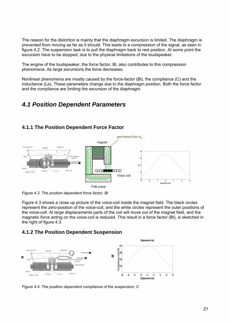
4.1.1 The Position Dependent Force Factor

Figure 4.3. The position dependent force factor, Bl Figure 4.3 shows a close up picture of the voice-coil inside the magnet field. The black circles represent the zero-position of the voice-coil, and the white circles represent the outer positions of the voice-coil. At large displacements parts of the coil will move out of the magnet field, and the magnetic force acting on the voice-coil is reduced. This result in a force factor (Bl), is sketched in the right of figure 4.3.

4.1.2 The Position Dependent Suspension Figure 4.4. The position dependent compliance of the suspension, C

-3 -2 -1 0 1 2 30

2

4

6

8

Excursion [mm]

Bl

Displacement [mm]

-8 -6 -4 -2 0 2 4 6 8

0.4

0.5

0.6

0.7

Displacement [mm]

Com

plia

nce

[mm

/N]

a b

22

Figure 4.4 shows the outer and inner suspension. In figure 4.4, b the position dependent compliance of the suspension is shown. The suspension is softest in the zero position of the voice-coil, and becomes less soft as the displacement increases. This is shown in figure 2.9,b.

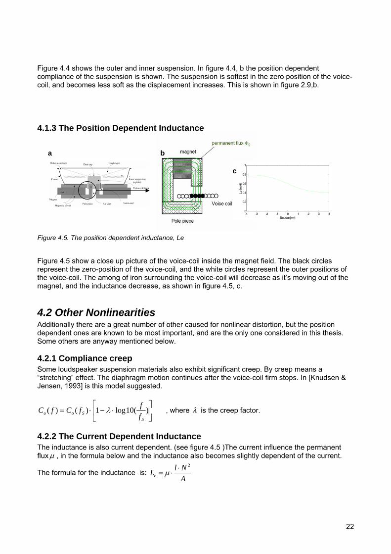
4.1.3 The Position Dependent Inductance Figure 4.5. The position dependent inductance, Le Figure 4.5 show a close up picture of the voice-coil inside the magnet field. The black circles represent the zero-position of the voice-coil, and the white circles represent the outer positions of the voice-coil. The among of iron surrounding the voice-coil will decrease as it’s moving out of the magnet, and the inductance decrease, as shown in figure 4.5, c.

4.2 Other Nonlinearities Additionally there are a great number of other caused for nonlinear distortion, but the position dependent ones are known to be most important, and are the only one considered in this thesis. Some others are anyway mentioned below.

4.2.1 Compliance creep Some loudspeaker suspension materials also exhibit significant creep. By creep means a “stretching” effect. The diaphragm motion continues after the voice-coil firm stops. In [Knudsen & Jensen, 1993] is this model suggested.

⎥⎦

⎤⎢⎣

⎡⋅−⋅= )(10log1)()(

SSoo f

ffCfC λ , where λ is the creep factor.

4.2.2 The Current Dependent Inductance The inductance is also current dependent. (see figure 4.5 )The current influence the permanent fluxμ , in the formula below and the inductance also becomes slightly dependent of the current.

The formula for the inductance is: ANlLe

2⋅⋅= μ

-4 -3 -2 -1 0 1 2 3 40

0.2

0.4

0.6

0.8

1

Excursion [mm]

Le [

mH

]

c

ba

23

where N is the number of turns of the voice-coil, A is the distance from the voice-coil to the magnet, and μ is the permanent flux in the magnet.

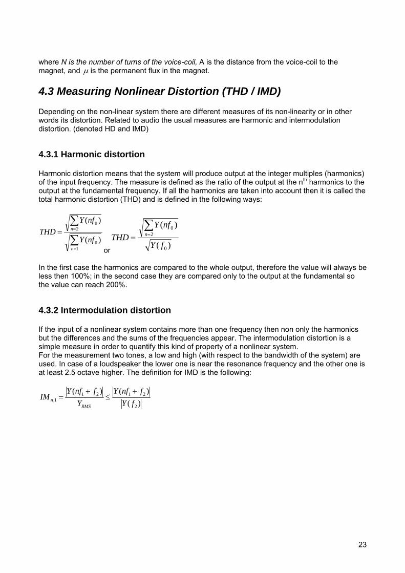
4.3 Measuring Nonlinear Distortion (THD / IMD)

Depending on the non-linear system there are different measures of its non-linearity or in other words its distortion. Related to audio the usual measures are harmonic and intermodulation distortion. (denoted HD and IMD)

4.3.1 Harmonic distortion

Harmonic distortion means that the system will produce output at the integer multiples (harmonics) of the input frequency. The measure is defined as the ratio of the output at the nth harmonics to the output at the fundamental frequency. If all the harmonics are taken into account then it is called the total harmonic distortion (THD) and is defined in the following ways:

∑

∑

=

==

10

20

)(

)(

n

n

nfY

nfYTHD

or )(

)(

0

20

fY

nfYTHD n

∑==

In the first case the harmonics are compared to the whole output, therefore the value will always be less then 100%; in the second case they are compared only to the output at the fundamental so the value can reach 200%.

4.3.2 Intermodulation distortion If the input of a nonlinear system contains more than one frequency then non only the harmonics but the differences and the sums of the frequencies appear. The intermodulation distortion is a simple measure in order to quantify this kind of property of a nonlinear system. For the measurement two tones, a low and high (with respect to the bandwidth of the system) are used. In case of a loudspeaker the lower one is near the resonance frequency and the other one is at least 2.5 octave higher. The definition for IMD is the following:

)()()(

2

21211, fY

fnfYY

fnfYIM

RMSn

+≤

+=

24

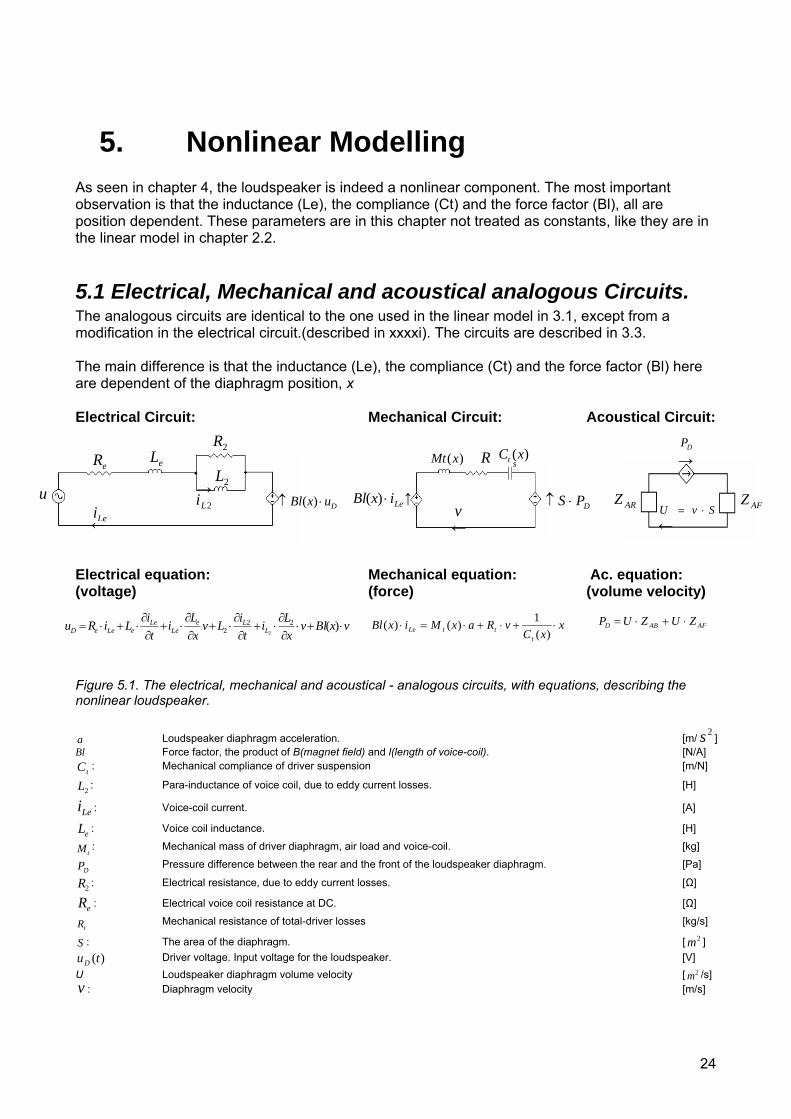
5. Nonlinear Modelling As seen in chapter 4, the loudspeaker is indeed a nonlinear component. The most important observation is that the inductance (Le), the compliance (Ct) and the force factor (Bl), all are position dependent. These parameters are in this chapter not treated as constants, like they are in the linear model in chapter 2.2.

5.1 Electrical, Mechanical and acoustical analogous Circuits. The analogous circuits are identical to the one used in the linear model in 3.1, except from a modification in the electrical circuit.(described in xxxxi). The circuits are described in 3.3. The main difference is that the inductance (Le), the compliance (Ct) and the force factor (Bl) here are dependent of the diaphragm position, x Electrical Circuit: Mechanical Circuit: Acoustical Circuit:

Electrical equation: Mechanical equation: Ac. equation: (voltage) (force) (volume velocity)

Figure 5.1. The electrical, mechanical and acoustical - analogous circuits, with equations, describing the nonlinear loudspeaker. a Loudspeaker diaphragm acceleration. [m/

2s ] Bl Force factor, the product of B(magnet field) and l(length of voice-coil). [N/A]


2L : Para-inductance of voice coil, due to eddy current losses. [H]





2R : Electrical resistance, due to eddy current losses. [Ω]



S : The area of the diaphragm. [ 2m ] )(tuD Driver voltage. Input voltage for the loudspeaker. [V]

U Loudspeaker diaphragm volume velocity [ 2m /s] v : Diaphragm velocity [m/s]

eR eL 2R

DuxBl ⋅↑ )(2Li

→ 2L u

Lei ←

)(xMt sR

LeixBl ⋅)( ↑ DPS ⋅↑

)(xCt

v ←

SvU ⋅=←

AFZ

DP→

ARZ

vxBlvxLi

tiLv

xL

it

iLiRu L

LeLe

LeeLeeD ⋅+⋅

∂∂⋅+

∂∂⋅+

∂∂⋅+

∂∂⋅+⋅= )(22

2 2x

xCvRaxMixBl

tttLe ⋅+⋅+⋅=⋅

)(1)()( AFABD ZUZUP ⋅+⋅=

25

cv : Voltage drop across the terminals of the voice coil / [V]



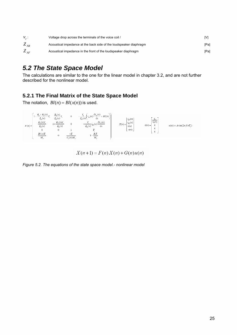
5.2 The State Space Model The calculations are similar to the one for the linear model in chapter 3.2, and are not further described for the nonlinear model.

5.2.1 The Final Matrix of the State Space Model The notation, ))(()( nxBlnBl = is used.

Figure 5.2. The equations of the state space model.- nonlinear model

26

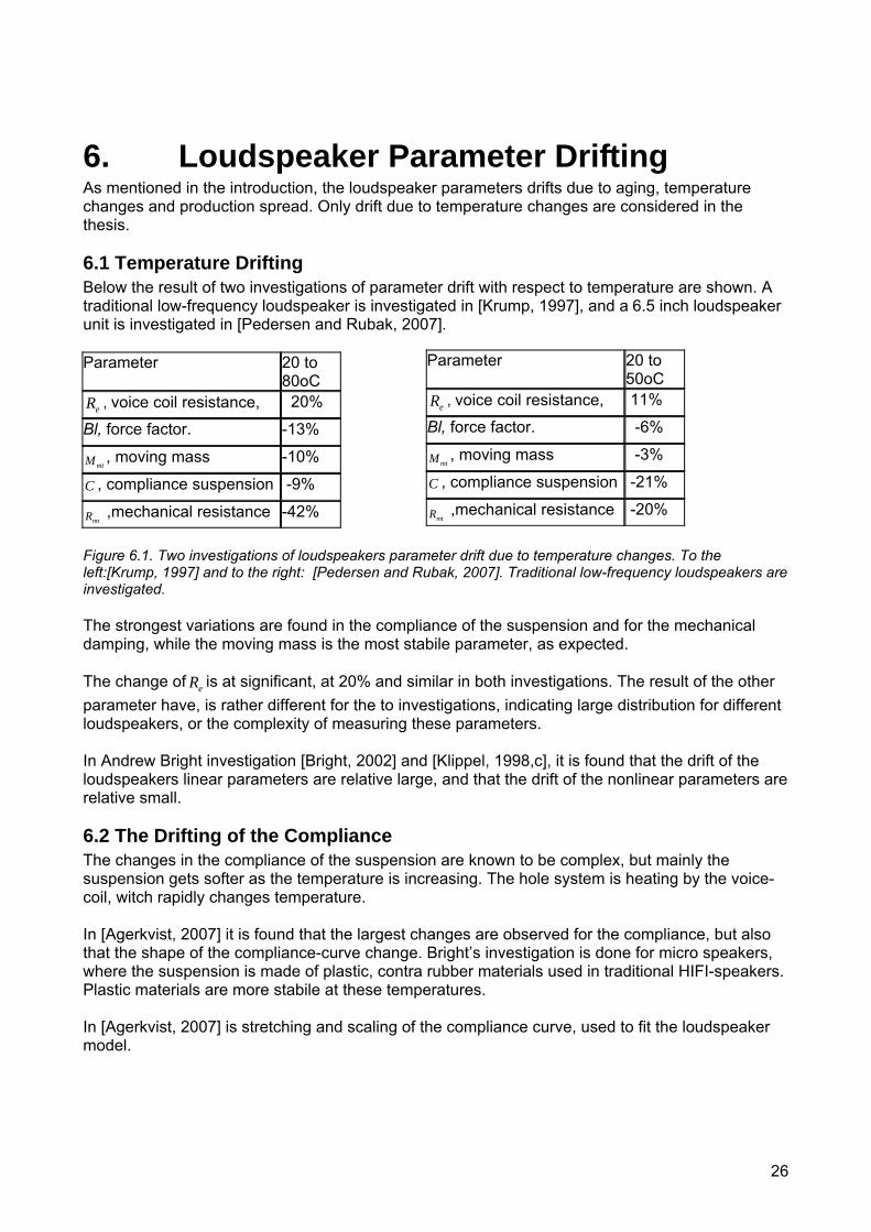
6. Loudspeaker Parameter Drifting As mentioned in the introduction, the loudspeaker parameters drifts due to aging, temperature changes and production spread. Only drift due to temperature changes are considered in the thesis.

6.1 Temperature Drifting Below the result of two investigations of parameter drift with respect to temperature are shown. A traditional low-frequency loudspeaker is investigated in [Krump, 1997], and a 6.5 inch loudspeaker unit is investigated in [Pedersen and Rubak, 2007]. Parameter 20 to

80oC eR , voice coil resistance, 20%

Bl, force factor. -13%

mtM , moving mass -10%

C , compliance suspension -9%

mtR ,mechanical resistance -42% Figure 6.1. Two investigations of loudspeakers parameter drift due to temperature changes. To the left:[Krump, 1997] and to the right: [Pedersen and Rubak, 2007]. Traditional low-frequency loudspeakers are investigated. The strongest variations are found in the compliance of the suspension and for the mechanical damping, while the moving mass is the most stabile parameter, as expected. The change of eR is at significant, at 20% and similar in both investigations. The result of the other parameter have, is rather different for the to investigations, indicating large distribution for different loudspeakers, or the complexity of measuring these parameters. In Andrew Bright investigation [Bright, 2002] and [Klippel, 1998,c], it is found that the drift of the loudspeakers linear parameters are relative large, and that the drift of the nonlinear parameters are relative small.

6.2 The Drifting of the Compliance The changes in the compliance of the suspension are known to be complex, but mainly the suspension gets softer as the temperature is increasing. The hole system is heating by the voice-coil, witch rapidly changes temperature. In [Agerkvist, 2007] it is found that the largest changes are observed for the compliance, but also that the shape of the compliance-curve change. Bright’s investigation is done for micro speakers, where the suspension is made of plastic, contra rubber materials used in traditional HIFI-speakers. Plastic materials are more stabile at these temperatures. In [Agerkvist, 2007] is stretching and scaling of the compliance curve, used to fit the loudspeaker model.

Parameter 20 to 50oC

eR , voice coil resistance, 11%

Bl, force factor. -6%

mtM , moving mass -3%

C , compliance suspension -21%

mtR ,mechanical resistance -20%

27

6.3 Updating the Loudspeaker Model - Due to Parameter Drifting Some kind of feedback from the loudspeaker is needed, to make the loudspeaker model able to follow the loudspeaker parameters drifting. Different papers suggest methods for updating the loudspeaker parameter, or often reefer to as “loudspeaker parameter identification”. In [Bright, 2002], a good overview is given. The most interesting methods use a current and voltage measurement as feedback, avoiding the traditionally problems due to motion measurements.(first described in [Klippel, 1998,c]) The impedance is analysed based on the voltage/current-measurement, and from the impedance can all the linear parameters is found. Further information can be found in [Bright, 2002].

28

7 Compensation of nonlinearities. (The content of this chapter is briefly described in the introduction.) There are three basic methods for compensation of nonlinearities, due to loudspeakers, or in general:

1. The negative feedback system. 2. The feedforward system. 3. The adaptive feedforward system.

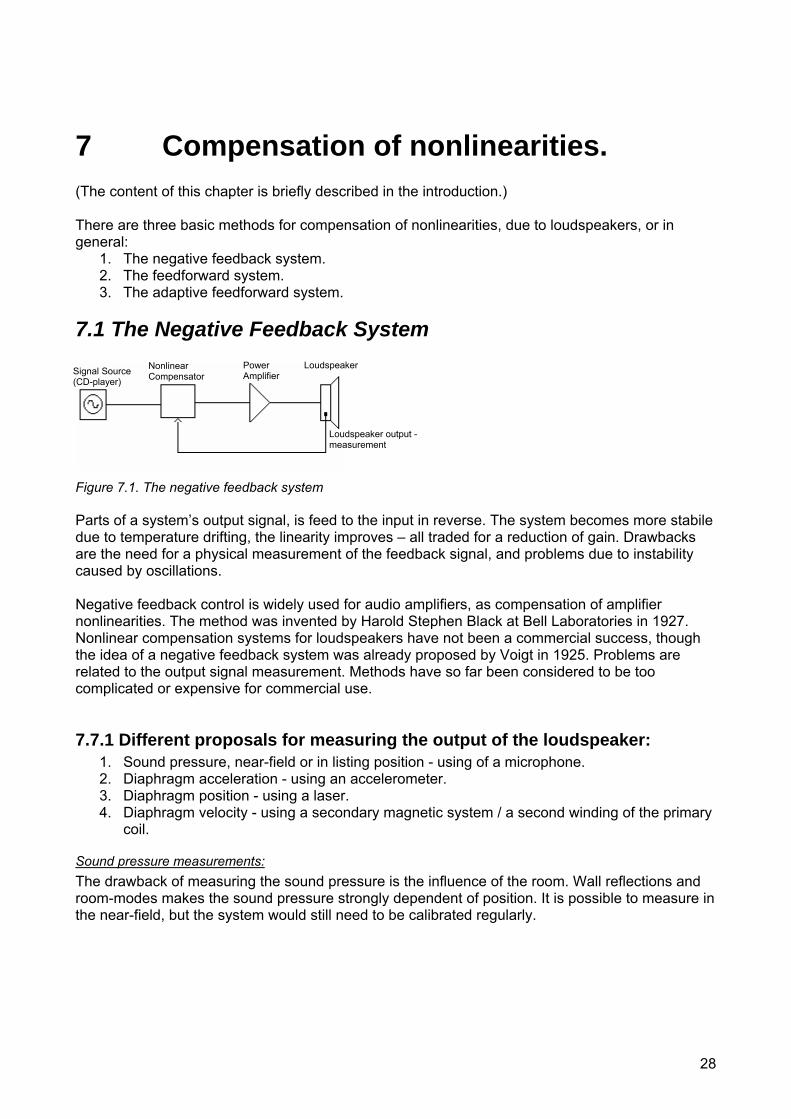
7.1 The Negative Feedback System

Figure 7.1. The negative feedback system Parts of a system’s output signal, is feed to the input in reverse. The system becomes more stabile due to temperature drifting, the linearity improves – all traded for a reduction of gain. Drawbacks are the need for a physical measurement of the feedback signal, and problems due to instability caused by oscillations. Negative feedback control is widely used for audio amplifiers, as compensation of amplifier nonlinearities. The method was invented by Harold Stephen Black at Bell Laboratories in 1927. Nonlinear compensation systems for loudspeakers have not been a commercial success, though the idea of a negative feedback system was already proposed by Voigt in 1925. Problems are related to the output signal measurement. Methods have so far been considered to be too complicated or expensive for commercial use.

7.7.1 Different proposals for measuring the output of the loudspeaker: 1. Sound pressure, near-field or in listing position - using of a microphone. 2. Diaphragm acceleration - using an accelerometer. 3. Diaphragm position - using a laser. 4. Diaphragm velocity - using a secondary magnetic system / a second winding of the primary

coil.

Sound pressure measurements: The drawback of measuring the sound pressure is the influence of the room. Wall reflections and room-modes makes the sound pressure strongly dependent of position. It is possible to measure in the near-field, but the system would still need to be calibrated regularly.



Power Amplifier

Loudspeaker

Loudspeaker output -measurement

29

Diaphragm measurement using an accelerometer Disadvantages with the system are the extra weight due to the accelerometer, and its traditionally high cost. Today accelerometers have become smaller, lighter and cheaper, making the whole concept far more actually. Still, just a smaller minority of subwoofer producers are using them as part of a negative feedback system. A reason for it could be that the need for calibration results in high production costs.

Diaphragm position measurement using a laser A laser measurement of the diaphragm position is the most accurate method available, but laser technology is too expensive for commercial use. It may be actual for real expensive active systems, with a laser placed inside the loudspeaker cabinet, measuring the rear side of the diaphragm.

Diaphragm velocity measurement using a secondary magnet system In 1927 Hanna published a description of a motion feedback system, using a secondary magnet system for monitoring the diaphragm velocity. A cheaper solution is to add a secondary winding to the primary coil.

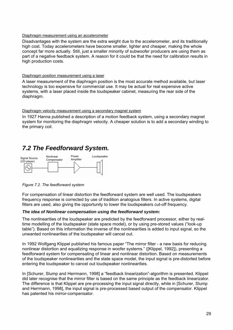
7.2 The Feedforward System.

Figure 7.2. The feedforward system For compensation of linear distortion the feedforward system are well used. The loudspeakers frequency response is corrected by use of tradition analogous filters. In active systems, digital filters are used, also giving the opportunity to lower the loudspeakers cut-off frequency.

The idea of Nonlinear compensation using the feedforward system: The nonlinearities of the loudspeaker are predicted by the feedforward processor, either by real-time modelling of the loudspeaker (state space model), or by using pre-stored values (“look-up table”). Based on this information the inverse of the nonlinearities is added to input signal, so the unwanted nonlinearities of the loudspeaker will cancel out. In 1992 Wolfgang Klippel published his famous paper “The mirror filter - a new basis for reducing nonlinear distortion and equalizing response in woofer systems.” ([Klippel, 1992]), presenting a feedforward system for compensating of linear and nonlinear distortion. Based on measurements of the loudspeaker nonlinearities and the state space model, the input signal is pre-distorted before entering the loudspeaker to cancel out loudspeaker nonlinearities. In [Schurer, Slump and Herrmann, 1998] a “feedback linearization”-algorithm is presented. Klippel did later recognise that the mirror filter is based on the same principle as the feedback linearizator. The difference is that Klippel are pre-processing the input signal directly, while in [Schurer, Slump and Herrmann, 1998], the input signal is pre-processed based output of the compensator. Klippel has patented his mirror-compensator.



Power Amplifier

Loudspeaker

30

The compensator algorithm in [Schurer, Slump and Herrmann, 1998] is chosen in for this project, and further described in 7.4). The quality of the compensation for a these pure feedforward systems totally depends on how accurate the loudspeaker model is. Drifting of loudspeaker parameters will reduce the performing, since no feedback is included.

7.3 The Adaptive Feedforward System.

Figure 7.3. The adaptive feedforward system Additionally to the pure feedforward system, a feedback signal from the loudspeaker is used for updating the parameters of the loudspeaker model, making the compensator able to handle loudspeaker parameters drifting. This is described in 6.3

7.4 The Chosen Compensation Algorithm. The feedback linearization in [Schurer, Slump and Herrmann, 1998], is chosen as compensator algorithm. In retrospect it is seen like a feedforward controller.

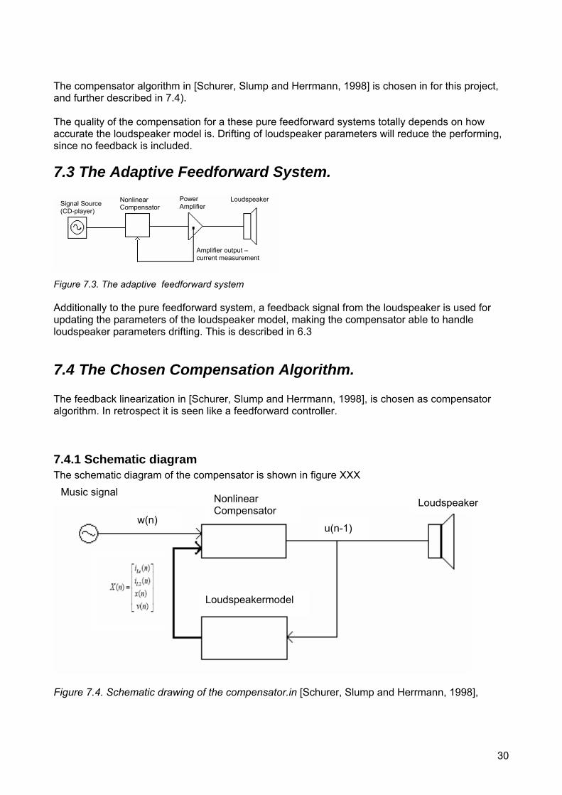
7.4.1 Schematic diagram The schematic diagram of the compensator is shown in figure XXX

Figure 7.4. Schematic drawing of the compensator.in [Schurer, Slump and Herrmann, 1998],



Power Amplifier

Loudspeaker

Amplifier output –current measurement


Loudspeakermodel

u(n-1) w(n)

Loudspeaker Music signal

31

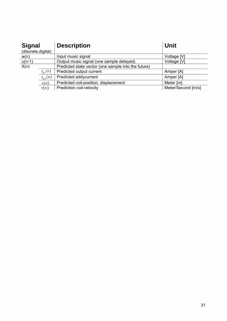
Signal (discrete,digital)

Description Unit w(n) Input music signal Voltage [V] u(n-1) Output music signal (one sample delayed) Voltage [V]

Predicted state vector (one sample into the future) Predicted output current Amper [A]

Predicted eddycurrent Amper [A] Predicted coil-position, displacement Meter [m]

X(n)

Prediction coil-velocity Meter/Second [m/s]

32

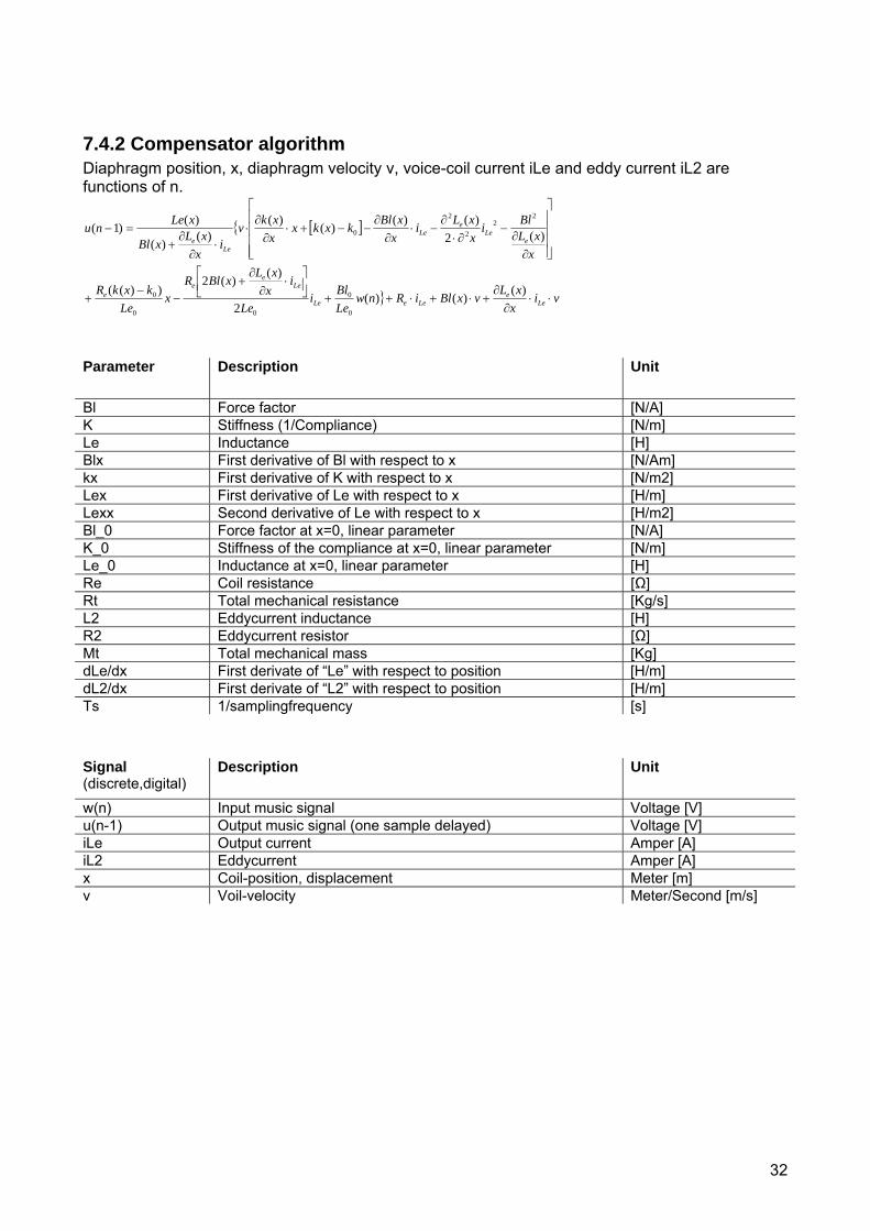
7.4.2 Compensator algorithm Diaphragm position, x, diaphragm velocity v, voice-coil current iLe and eddy current iL2 are functions of n.

[ ]

vixxLvxBliRnw

LeBli

Le

ixxLxBlR

xLe

kxkR

xxL

BlixxLi

xxBlkxkx

xxkv

ixxLxBl

xLenu

Lee

LeeLe

Lee

ee

eLe

eLe

Lee

⋅⋅∂

∂+⋅+⋅++

⎥⎦⎤

⎢⎣⎡ ⋅

∂∂

+−

−+

⎥⎥⎥⎥

⎦

⎤

⎢⎢⎢⎢

⎣

⎡

∂∂

−∂⋅

∂−⋅

∂∂

−−+⋅∂

∂⋅

⋅∂

∂+

=−

)()()(2

)()(2))((

)(2)()()()(

)()(

)()1(

0

0

00

0

22

2

2

0

Signal (discrete,digital)

Description Unit

w(n) Input music signal Voltage [V] u(n-1) Output music signal (one sample delayed) Voltage [V] iLe Output current Amper [A] iL2 Eddycurrent Amper [A] x Coil-position, displacement Meter [m] v Voil-velocity Meter/Second [m/s]

Parameter Description Unit

Bl Force factor [N/A] K Stiffness (1/Compliance) [N/m] Le Inductance [H] Blx First derivative of Bl with respect to x [N/Am] kx First derivative of K with respect to x [N/m2] Lex First derivative of Le with respect to x [H/m] Lexx Second derivative of Le with respect to x [H/m2] Bl_0 Force factor at x=0, linear parameter [N/A] K_0 Stiffness of the compliance at x=0, linear parameter [N/m] Le_0 Inductance at x=0, linear parameter [H] Re Coil resistance [Ω] Rt Total mechanical resistance [Kg/s] L2 Eddycurrent inductance [H] R2 Eddycurrent resistor [Ω] Mt Total mechanical mass [Kg] dLe/dx First derivate of “Le” with respect to position [H/m] dL2/dx First derivate of “L2” with respect to position [H/m] Ts 1/samplingfrequency [s]

33

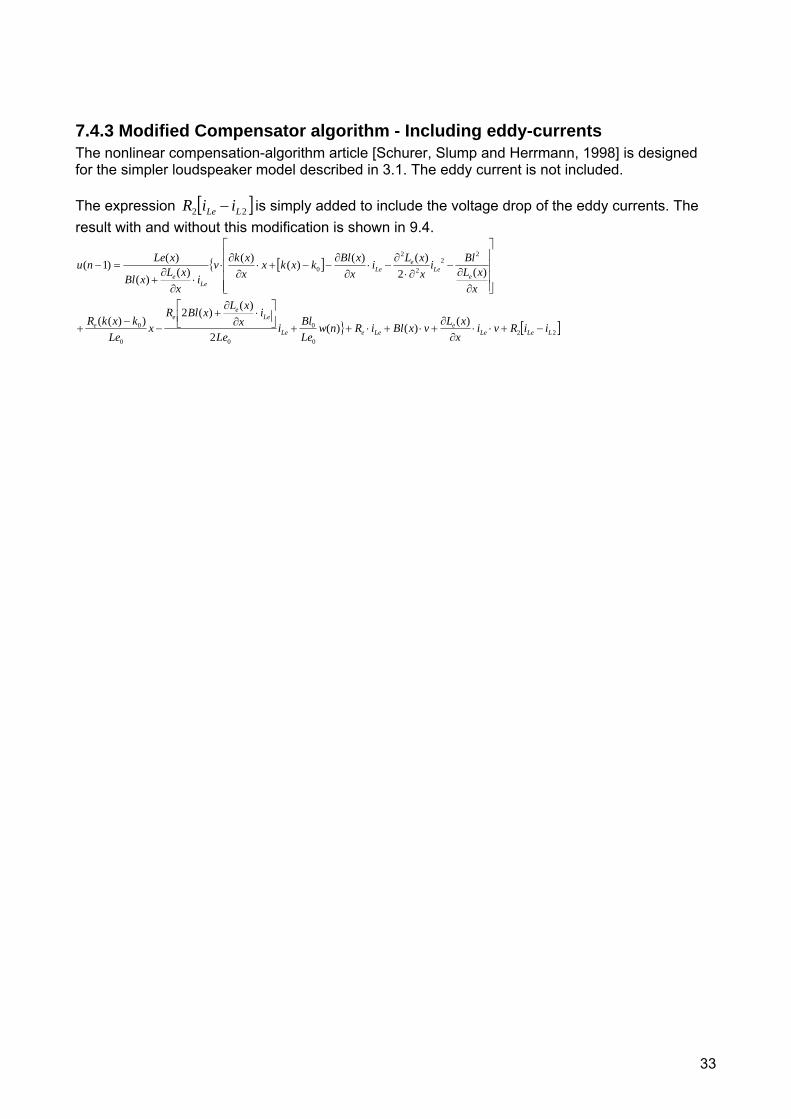
7.4.3 Modified Compensator algorithm - Including eddy-currents The nonlinear compensation-algorithm article [Schurer, Slump and Herrmann, 1998] is designed for the simpler loudspeaker model described in 3.1. The eddy current is not included. The expression [ ]22 LLe iiR − is simply added to include the voltage drop of the eddy currents. The result with and without this modification is shown in 9.4.

[ ]

[ ]220

0

00

0

22

2

2

0

)()()(2

)()(2))((

)(2)()()()(

)()(

)()1(

LLeLee

LeeLe

Lee

ee

eLe

eLe

Lee

iiRvixxLvxBliRnw

LeBli

Le

ixxLxBlR

xLe

kxkR

xxL

BlixxLi

xxBlkxkx

xxkv

ixxLxBl

xLenu

−+⋅⋅∂

∂+⋅+⋅++

⎥⎦⎤

⎢⎣⎡ ⋅

∂∂

+−

−+

⎥⎥⎥⎥

⎦

⎤

⎢⎢⎢⎢

⎣

⎡

∂∂

−∂⋅

∂−⋅

∂∂

−−+⋅∂

∂⋅

⋅∂

∂+

=−

34

8. Loudspeaker - Measurements

8.1 Loudspeaker Parameters Measurement

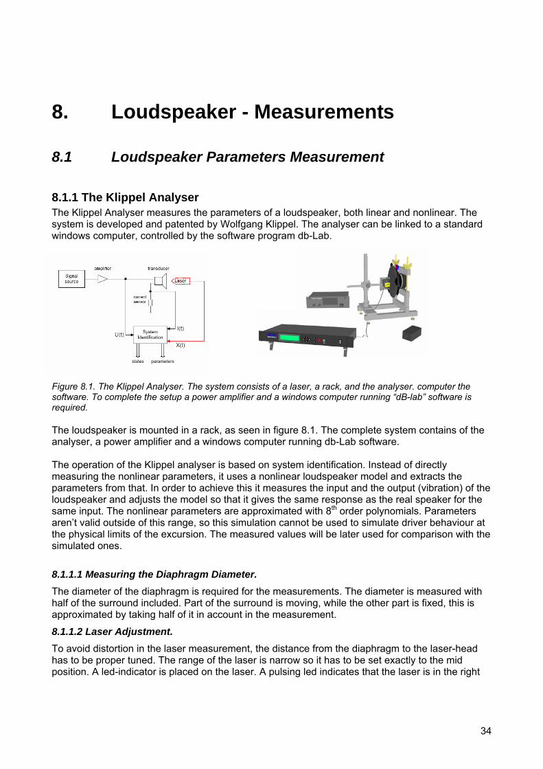
8.1.1 The Klippel Analyser The Klippel Analyser measures the parameters of a loudspeaker, both linear and nonlinear. The system is developed and patented by Wolfgang Klippel. The analyser can be linked to a standard windows computer, controlled by the software program db-Lab.

Figure 8.1. The Klippel Analyser. The system consists of a laser, a rack, and the analyser. computer the software. To complete the setup a power amplifier and a windows computer running “dB-lab” software is required. The loudspeaker is mounted in a rack, as seen in figure 8.1. The complete system contains of the analyser, a power amplifier and a windows computer running db-Lab software. The operation of the Klippel analyser is based on system identification. Instead of directly measuring the nonlinear parameters, it uses a nonlinear loudspeaker model and extracts the parameters from that. In order to achieve this it measures the input and the output (vibration) of the loudspeaker and adjusts the model so that it gives the same response as the real speaker for the same input. The nonlinear parameters are approximated with 8th order polynomials. Parameters aren’t valid outside of this range, so this simulation cannot be used to simulate driver behaviour at the physical limits of the excursion. The measured values will be later used for comparison with the simulated ones.

8.1.1.1 Measuring the Diaphragm Diameter. The diameter of the diaphragm is required for the measurements. The diameter is measured with half of the surround included. Part of the surround is moving, while the other part is fixed, this is approximated by taking half of it in account in the measurement.

8.1.1.2 Laser Adjustment. To avoid distortion in the laser measurement, the distance from the diaphragm to the laser-head has to be proper tuned. The range of the laser is narrow so it has to be set exactly to the mid position. A led-indicator is placed on the laser. A pulsing led indicates that the laser is in the right

35

area, but still out of range. Just where the led changes from pulsing to permanently lightning, indicates the outer position. The optimal laser position is between the two outer positions.

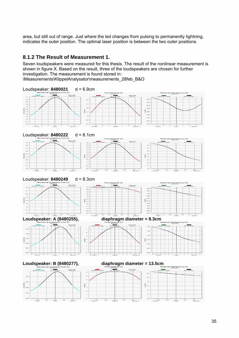
8.1.2 The Result of Measurement 1. Seven loudspeakers were measured for this thesis. The result of the nonlinear measurement is shown in figure X. Based on the result, three of the loudspeakers are chosen for further investigation. The measurement is found stored in: \Measurements\KlippelAnalysator\measurements_28feb_B&O Loudspeaker: 8480021 d = 6.9cm

Loudspeaker: 8480222 d = 8.1cm

Loudspeaker: 8480249 d = 8.3cm

Loudspeaker: A (8480255), diaphragm diameter = 8.3cm

Loudspeaker: B (8480277), diaphragm diameter = 13.5cm

36

Loudspeaker: C (8480285), diaphragm diameter = 10.0cm

Loudspeaker: Tymphany 205-116 QC.131005 d = 20.7cm

Figure 8.2 The result of measurement 1- nonlinear parameters. The black lines are the measured result and the colour lines are the polynom fitting done by the klippel analysator.

8.1.2.1 Measurement result. The black lines are the measured result and the colour line is the polynom fitting done by the klippel analysator, to model the parameters. These polynomes are later used in the loudspeaker modelling. The measured inductance for loudspeaker:848002, not seems to be reliable, due to that the inductance increases with displacement. When the voice coil is moving away from the magnet, the inductance should decrease, due to the description in 4.1.3. The measured force-factor for loudspeaker:84800249 is also a bit strange. The force factor should also decrease when the voice-coil is moving away from the magnet gap, due to the description in 4.1.1. The loudspeakers who is chosen for futher investigation is

• “Loudspeaker A” - has a relatively symmetric Bl-factor and an unsymmetrical compliance. • “Loudspeaker B” has both a relatively symmetric Bl-factor and compliance. • “Loudspeaker C” has a relatively unsymmetrical Bl-factor and a symmetrical compliance.

37

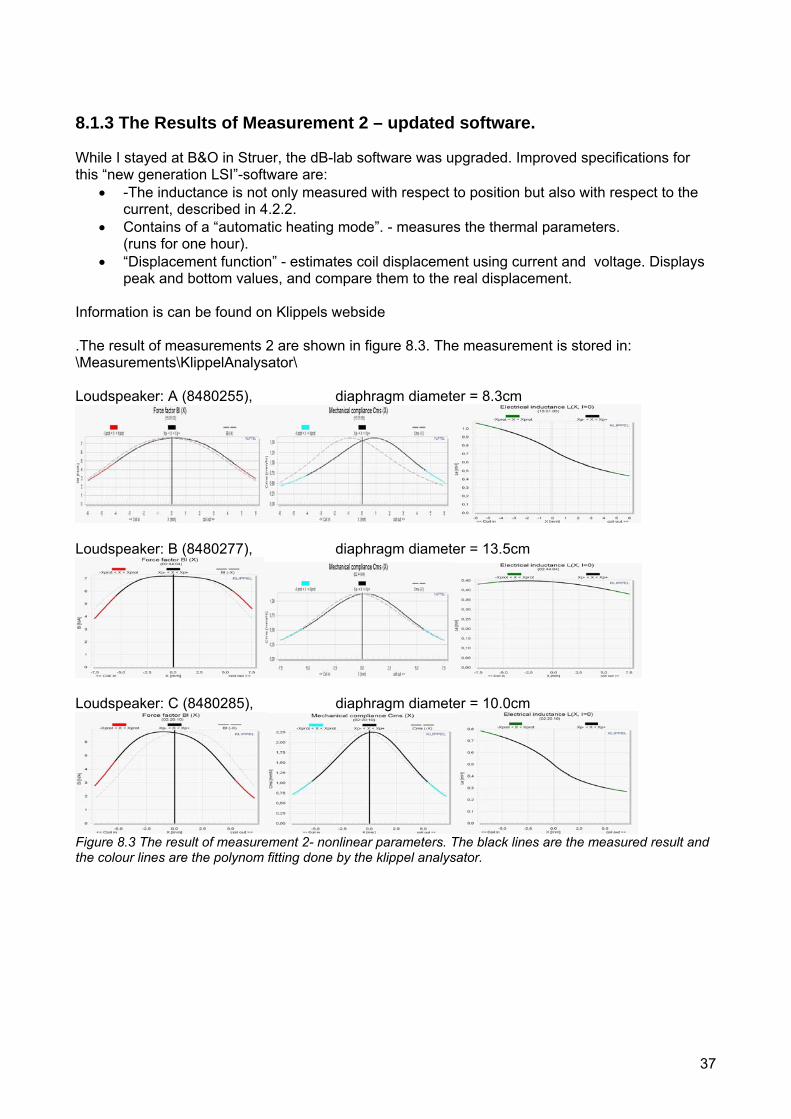
8.1.3 The Results of Measurement 2 – updated software. While I stayed at B&O in Struer, the dB-lab software was upgraded. Improved specifications for this “new generation LSI”-software are:

• -The inductance is not only measured with respect to position but also with respect to the current, described in 4.2.2.

• Contains of a “automatic heating mode”. - measures the thermal parameters. (runs for one hour).

• “Displacement function” - estimates coil displacement using current and voltage. Displays peak and bottom values, and compare them to the real displacement.

Information is can be found on Klippels webside .The result of measurements 2 are shown in figure 8.3. The measurement is stored in: \Measurements\KlippelAnalysator\ Loudspeaker: A (8480255), diaphragm diameter = 8.3cm


Loudspeaker: C (8480285), diaphragm diameter = 10.0cm

Figure 8.3 The result of measurement 2- nonlinear parameters. The black lines are the measured result and the colour lines are the polynom fitting done by the klippel analysator.

38

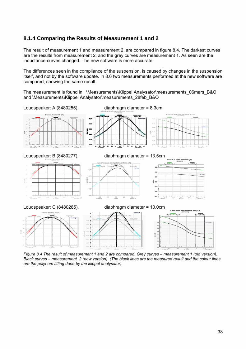
8.1.4 Comparing the Results of Measurement 1 and 2 The result of measurement 1 and measurement 2, are compared in figure 8.4. The darkest curves are the results from measurement 2, and the grey curves are measurement 1. As seen are the inductance-curves changed. The new software is more accurate. The differences seen in the compliance of the suspension, is caused by changes in the suspension itself, and not by the software update. In 8.6 two measurements performed at the new software are compared, showing the same result. The measurement is found in \Measurements\Klippel Analysator\measurements_06mars_B&O and \Measurements\Klippel Analysator\measurements_28feb_B&O Loudspeaker: A (8480255), diaphragm diameter = 8.3cm


Loudspeaker: C (8480285), diaphragm diameter = 10.0cm Figure 8.4 The result of measurement 1 and 2 are compared. Grey curves – measurement 1 (old version). Black curves – measurement 2 (new version) (The black lines are the measured result and the colour lines are the polynom fitting done by the klippel analysator).

39

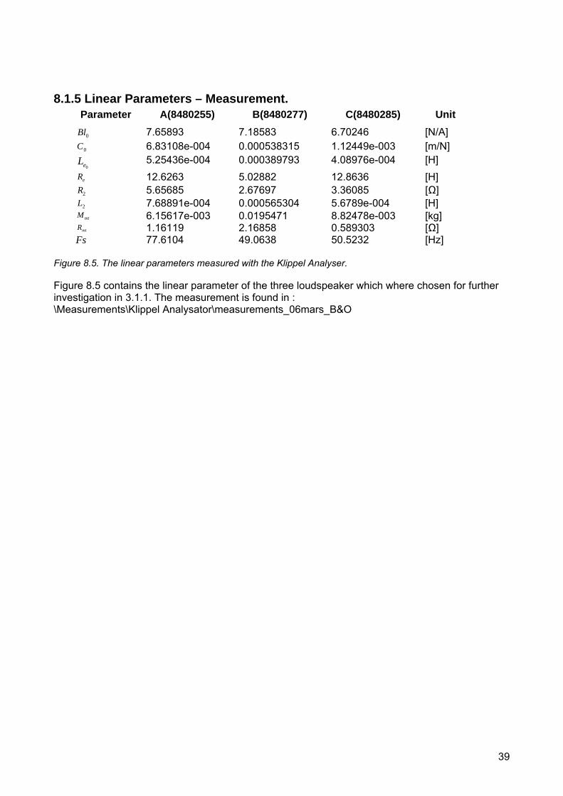
8.1.5 Linear Parameters – Measurement. Parameter A(8480255) B(8480277) C(8480285) Unit

0Bl 7.65893 7.18583 6.70246 [N/A] 0C 6.83108e-004 0.000538315 1.12449e-003 [m/N]

0eL 5.25436e-004 0.000389793 4.08976e-004 [H]

eR 12.6263 5.02882 12.8636 [H] 2R 5.65685 2.67697 3.36085 [Ω] 2L 7.68891e-004 0.000565304 5.6789e-004 [H] mtM 6.15617e-003 0.0195471 8.82478e-003 [kg]

mtR 1.16119 2.16858 0.589303 [Ω] Fs 77.6104 49.0638 50.5232 [Hz]

Figure 8.5. The linear parameters measured with the Klippel Analyser. Figure 8.5 contains the linear parameter of the three loudspeaker which where chosen for further investigation in 3.1.1. The measurement is found in : \Measurements\Klippel Analysator\measurements_06mars_B&O

40

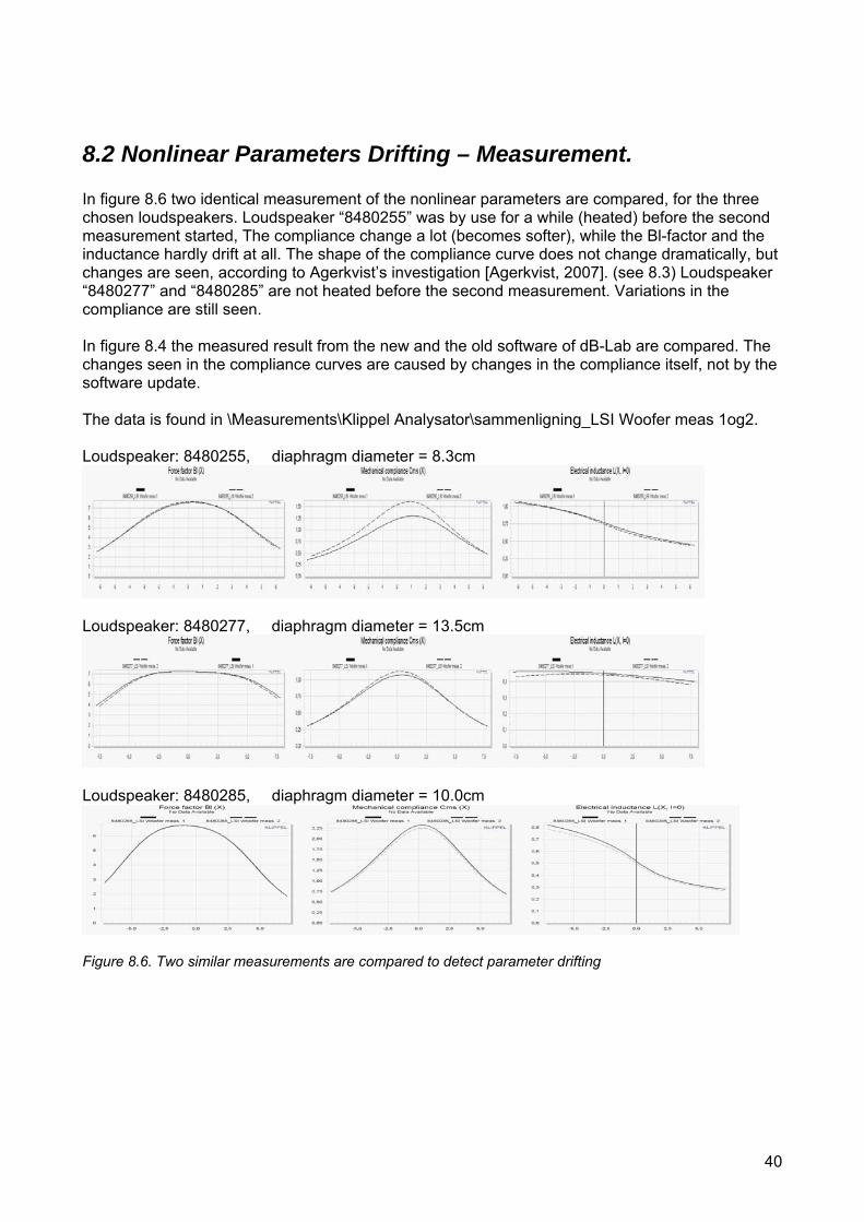
8.2 Nonlinear Parameters Drifting – Measurement. In figure 8.6 two identical measurement of the nonlinear parameters are compared, for the three chosen loudspeakers. Loudspeaker “8480255” was by use for a while (heated) before the second measurement started, The compliance change a lot (becomes softer), while the Bl-factor and the inductance hardly drift at all. The shape of the compliance curve does not change dramatically, but changes are seen, according to Agerkvist’s investigation [Agerkvist, 2007]. (see 8.3) Loudspeaker “8480277” and “8480285” are not heated before the second measurement. Variations in the compliance are still seen. In figure 8.4 the measured result from the new and the old software of dB-Lab are compared. The changes seen in the compliance curves are caused by changes in the compliance itself, not by the software update. The data is found in \Measurements\Klippel Analysator\sammenligning_LSI Woofer meas 1og2. Loudspeaker: 8480255, diaphragm diameter = 8.3cm

Loudspeaker: 8480277, diaphragm diameter = 13.5cm

Loudspeaker: 8480285, diaphragm diameter = 10.0cm

Figure 8.6. Two similar measurements are compared to detect parameter drifting

41

8.3 Loudspeaker Output Measurement – Displacement.

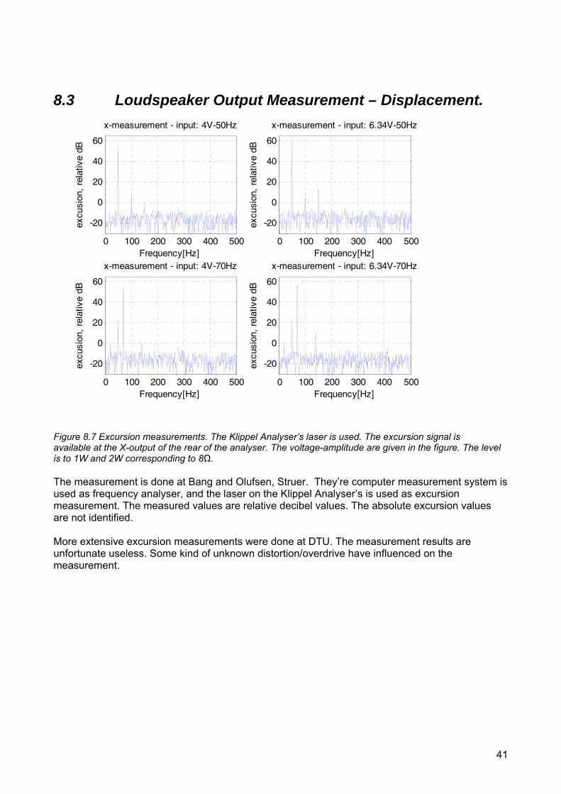
Figure 8.7 Excursion measurements. The Klippel Analyser’s laser is used. The excursion signal is available at the X-output of the rear of the analyser. The voltage-amplitude are given in the figure. The level is to 1W and 2W corresponding to 8Ω. The measurement is done at Bang and Olufsen, Struer. They’re computer measurement system is used as frequency analyser, and the laser on the Klippel Analyser’s is used as excursion measurement. The measured values are relative decibel values. The absolute excursion values are not identified. More extensive excursion measurements were done at DTU. The measurement results are unfortunate useless. Some kind of unknown distortion/overdrive have influenced on the measurement.

0 100 200 300 400 500

-20

0

20

40

60

Frequency[Hz]

excu

sion

, re

lativ

e dB

x-measurement - input: 4V-50Hz

0 100 200 300 400 500

-20

0

20

40

60

Frequency[Hz]ex

cusi

on,

rela

tive

dB

x-measurement - input: 6.34V-50Hz

0 100 200 300 400 500

-20

0

20

40

60

Frequency[Hz]

excu

sion

, re

lativ

e dB

x-measurement - input: 4V-70Hz

0 100 200 300 400 500

-20

0

20

40

60

Frequency[Hz]

excu

sion

, re

lativ

e dB

x-measurement - input: 6.34V-70Hz

42

9. Matlab simulation

9.1 Overview of Matlab functions 9.1.1 Linear_Loudspeaker_Model_Simplified Appendix A1 Simulation of the linear model in 3.2.6. 9.1.2 Nonlinear_Loudspeaker_Model_Simplified Appendix A2 Simulation of the nonlinear model without eddycurrent, The model in 3.2.6 is used with nonlinear parameters (Bl(x), C(x) and Le(x)) 9.1.4 Nonlinear_Loudspeaker_Model Appendix A3 Simulation of the nonlinear model in 5.2.1.. 9.1.5 Nonlinear_Compensator_Simplified Appendix A4 Simulation of the nonlinear compensation algorithm in 7.4.2 9.1.6 Nonlinear_Compensator Appendix A5 Simulation of the nonlinear compensation algorithm in 7.4.3 9.1.7 Compliance_Adjustment Appendix A6 Stretching and scaling the compliance curve 9.1.8 THD_Calculator Appendix A7 Function for the THD-calculation due to 4.3.1 9.1.9 IMD_Calculator Appendix A8 Function for the IMD-calculation in 4.3.2 9.1.10 Load_Nonlinear_Parameters Appendix A9 Loading polynomials & Generating tables for the nonlinear parameters 9.1.11 Load_Linear_Parameters Appendix A10 Loading linear parameter 9.1.12 Plot_Nonlinear_Parameter Appendix A11 Plot the curves of the nonlinear parameters 9.1.13 Capture.m Appendix A12 VisualAudio to Matlab interface, previous developed at B&O 9.1.14 Main.m Appendix A13 Script to call the other functions call

43

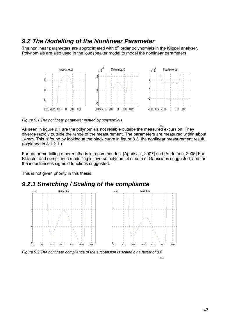
9.2 The Modelling of the Nonlinear Parameter The nonlinear parameters are approximated with 8th order polynomials in the Klippel analyser. Polynomials are also used in the loudspeaker model to model the nonlinear parameters.

Figure 9.1 The nonlinear parameter plotted by polynomials As seen in figure 9.1 are the polynomials not reliable outside the measured excursion. They diverge rapidly outside the range of the measurement. The parameters are measured within about ±4mm. This is found by looking at the black curve in figure 8.3, the nonlinear measurement result. (explaned in 8.1.2.1 ) For better modelling other methods is recommended. [Agerkvist, 2007] and [Andersen, 2005] For Bl-factor and compliance modelling is inverse polynomial or sum of Gaussians suggested, and for the inductance is sigmoid functions suggested. This is not given priority in this thesis.

9.2.1 Stretching / Scaling of the compliance

0 500 1000 1500 2000 2500 30000

1

2

x 10-4 Orginal, Cms

0 500 1000 1500 2000 2500 30000

1

2

x 10-4 tuned, Cms

Figure 9.2 The nonlinear compliance of the suspension is scaled by a factor of 0.8

ddLe

-0.03 -0.02 -0.01 0 0.01 0.02

-5

0

5

Force-factor,Bl

-0.03 -0.02 -0.01 0 0.01 0.02

-2

0

2

x 10-3 Compliance, C

-0.03 -0.02 -0.01 0 0.01 0.02

-5

0

5

x 10-4 Inductance, Le

ddLe

44

0 500 1000 1500 2000 2500 30000

1

2

x 10-4 Orginal, Cms

0 500 1000 1500 2000 2500 30000

1

2

x 10-4 tuned, Cms

Figure 9.3 The nonlinear compliance of the suspension is stretched by a factor of 0.8 Since the compliance is the parameter that is mostly drifting, these simple adjustment technique is used to fit the loudspeaker model to the loudspeaker.

9.3 The Loudspeaker Model

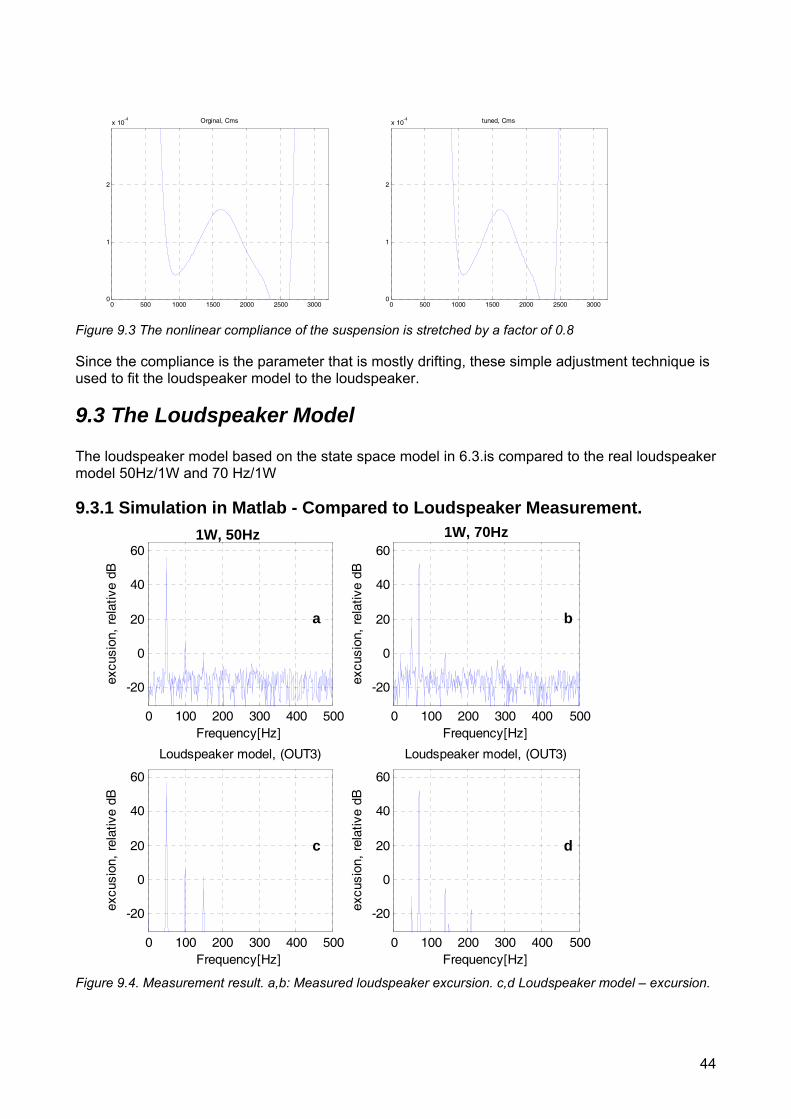
The loudspeaker model based on the state space model in 6.3.is compared to the real loudspeaker model 50Hz/1W and 70 Hz/1W

9.3.1 Simulation in Matlab - Compared to Loudspeaker Measurement.

0 100 200 300 400 500

-20

0

20

40

60

Frequency[Hz]

excu

sion

, re

lativ

e dB

0 100 200 300 400 500

-20

0

20

40

60

Frequency[Hz]

excu

sion

, re

lativ

e dB

0 100 200 300 400 500

-20

0

20

40

60

Frequency[Hz]

excu

sion

, re

lativ

e dB

Loudspeaker model, (OUT3)

0 100 200 300 400 500

-20

0

20

40

60

Frequency[Hz]

excu

sion

, re

lativ

e dB


Figure 9.4. Measurement result. a,b: Measured loudspeaker excursion. c,d Loudspeaker model – excursion.

1W, 50Hz 1W, 70Hz

a b

c d

45

The measurement is done at Bang and Olufsen, Struer. They’re computer measurement system is used as frequency analyser, and the laser on the Klippel Analyser’s is used as excursion measurement. The measured values are relative decibel values. The absolute excursion values are not identified. As seen in the figure below does the loudspeaker model fit the loudspeaker pretty well. The difference for the second harmonic is 0.8 dB is

“Absolute values” 50Hz, 1W Fundamental 2. harmonic 3.harmonic Loudspeaker 56,2 5,9 0,7 Loudspeaker model 57 5,9 1,5 (Data is collected from: \Measurement_result\FinalTest) Relative values (the fundamental is scaled to 0 dB)

1W -70Hz The loudspeaker model does not fit the loudspeaker. The harmonics are underestimated in the loudspeaker model.

Absolute values

Relative values (the fundamental is scaled to 0 dB

50Hz, 1W Fundamental 2. harmonic 3.harmonic Loudspeaker 0 -50.3 -55.5 Loudspeaker model 0 -51.1 -55,5

70Hz, 1W Fundamental 2. harmonic 4.harmonic Loudspeaker 52,7 0,8 3.3 Loudspeaker model 52,6 -5,2 -

70Hz, 1W Fundamental 2. harmonic 4.harmonic Loudspeaker 0 -51.9 -56 Loudspeaker model 0 -57.8 -

46

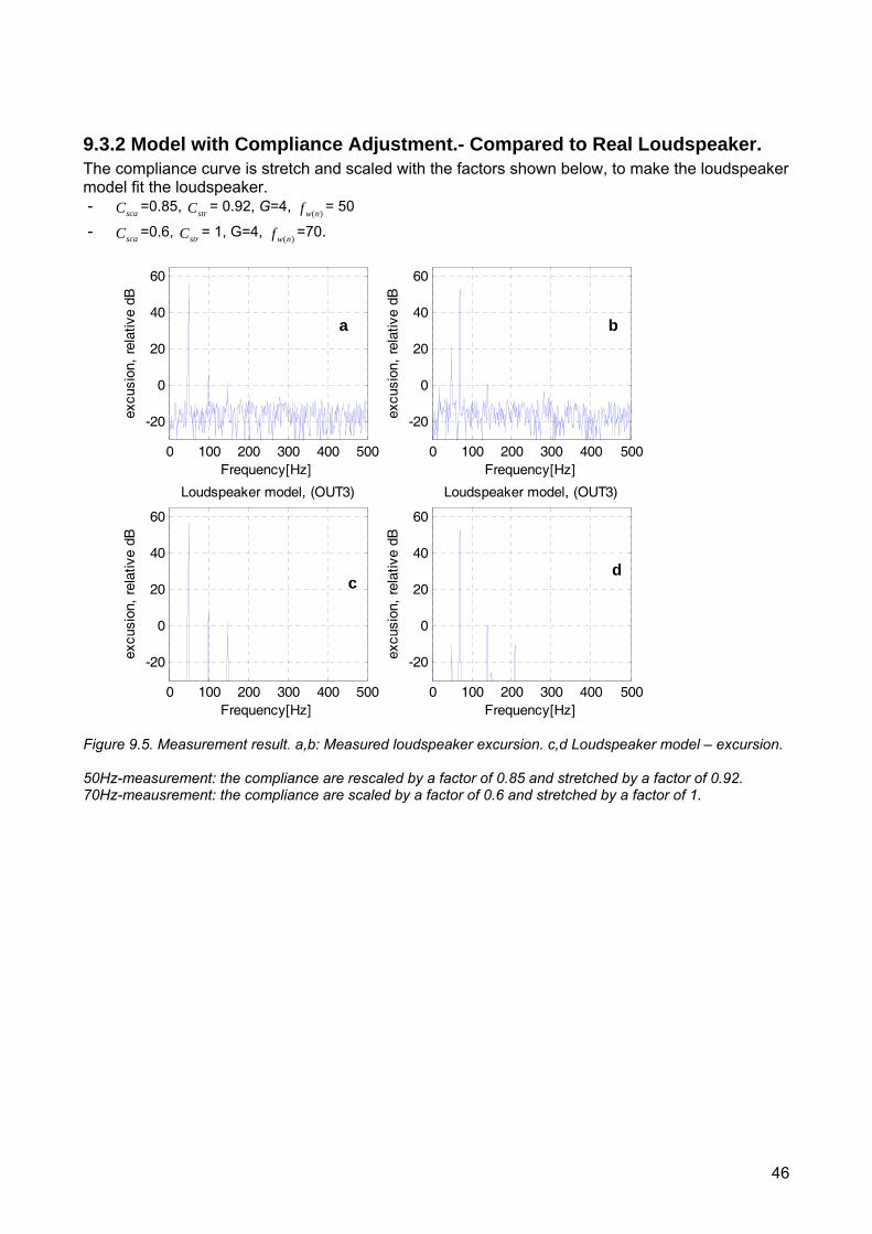
9.3.2 Model with Compliance Adjustment.- Compared to Real Loudspeaker. The compliance curve is stretch and scaled with the factors shown below, to make the loudspeaker model fit the loudspeaker. - scaC =0.85, strC = 0.92, G=4, )(nwf = 50 - scaC =0.6, strC = 1, G=4, )(nwf =70.

Figure 9.5. Measurement result. a,b: Measured loudspeaker excursion. c,d Loudspeaker model – excursion. 50Hz-measurement: the compliance are rescaled by a factor of 0.85 and stretched by a factor of 0.92. 70Hz-meausrement: the compliance are scaled by a factor of 0.6 and stretched by a factor of 1.

0 100 200 300 400 500

-20

0

20

40

60

Frequency[Hz]

excu

sion

, re

lativ

e dB

0 100 200 300 400 500

-20

0

20

40

60

Frequency[Hz]

excu

sion

, re

lativ

e dB

0 100 200 300 400 500

-20

0

20

40

60

Frequency[Hz]

excu

sion

, re

lativ

e dB


0 100 200 300 400 500

-20

0

20

40

60

Frequency[Hz]

excu

sion

, re

lativ

e dB


a b

c d

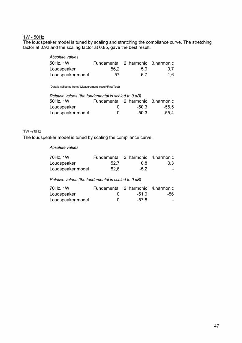
47

1W - 50Hz The loudspeaker model is tuned by scaling and stretching the compliance curve. The stretching factor at 0.92 and the scaling factor at 0.85, gave the best result.

Absolute values

(Data is collected from: \Measurement_result\FinalTest)

Relative values (the fundamental is scaled to 0 dB)

1W -70Hz The loudspeaker model is tuned by scaling the compliance curve.

Absolute values


50Hz, 1W Fundamental 2. harmonic 3.harmonic Loudspeaker 56,2 5,9 0,7 Loudspeaker model 57 6.7 1,6

50Hz, 1W Fundamental 2. harmonic 3.harmonic Loudspeaker 0 -50.3 -55.5 Loudspeaker model 0 -50.3 -55,4

70Hz, 1W Fundamental 2. harmonic 4.harmonic Loudspeaker 52,7 0,8 3.3 Loudspeaker model 52,6 -5,2 -

70Hz, 1W Fundamental 2. harmonic 4.harmonic Loudspeaker 0 -51.9 -56 Loudspeaker model 0 -57.8 -

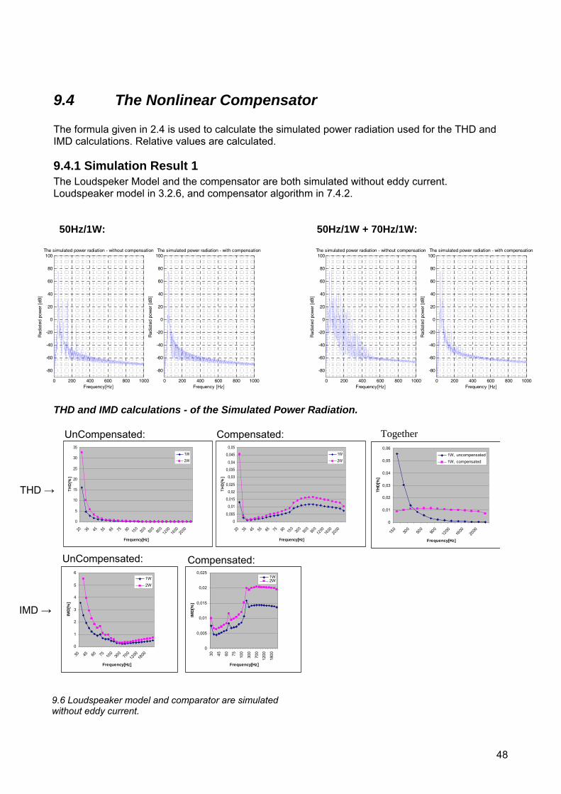
48

9.4 The Nonlinear Compensator The formula given in 2.4 is used to calculate the simulated power radiation used for the THD and IMD calculations. Relative values are calculated.

9.4.1 Simulation Result 1 The Loudspeker Model and the compensator are both simulated without eddy current. Loudspeaker model in 3.2.6, and compensator algorithm in 7.4.2. 50Hz/1W: 50Hz/1W + 70Hz/1W:

THD and IMD calculations - of the Simulated Power Radiation.

0

5

10

15

20

25

30

35

20 35 45 55 65 75 90 150

300

500

900

1200

1600

2000

Frequency[Hz]

THD[

%]

1W2W

0

0,005

0,01

0,015

0,02

0,025

0,03

0,035

0,04

0,045

0,05

20 35 45 55 65 75 90 150

300

500

900

1200

1600

2000

Frequency[Hz]

THD[

%]

1W2W

0

0,01

0,02

0,03

0,04

0,05

0,06

150

300

500

900

1200

1600

2000

Frequency[Hz]

THD[

%]

1W, uncompensated1W, compensated

THD →

0

1

2

3

4

5

6

30 45 60 75 100

300

700

1200

1800

Frequency[Hz]

IMD

[%]

1W2W

0

0,005

0,01

0,015

0,02

0,025

30 45 60 75 100

300

700

1200

1800

Frequency[Hz]

IMD

[%]

1W2W

IMD →

Compensated: UnCompensated:

UnCompensated: Compensated:

0 200 400 600 800 1000

-80

-60

-40

-20

0

20

40

60

80

100The simulated power radiation - without compensation

Rad

iate

d po

wer

[dB

]

Frequency[Hz]0 200 400 600 800 1000

-80

-60

-40

-20

0

20

40

60

80

100The simulated power radiation - with compensation

Rad

iate

d po

wer

[dB

]

Frequency [Hz]0 200 400 600 800 1000

-80

-60

-40

-20

0

20

40

60

80


Rad

iate

d po

wer

[dB

]

Frequency[Hz]0 200 400 600 800 1000

-80

-60

-40

-20

0

20

40

60

80


Rad

iate

d po

wer

[dB

]

Frequency [Hz]

Together

9.6 Loudspeaker model and comparator are simulated without eddy current.

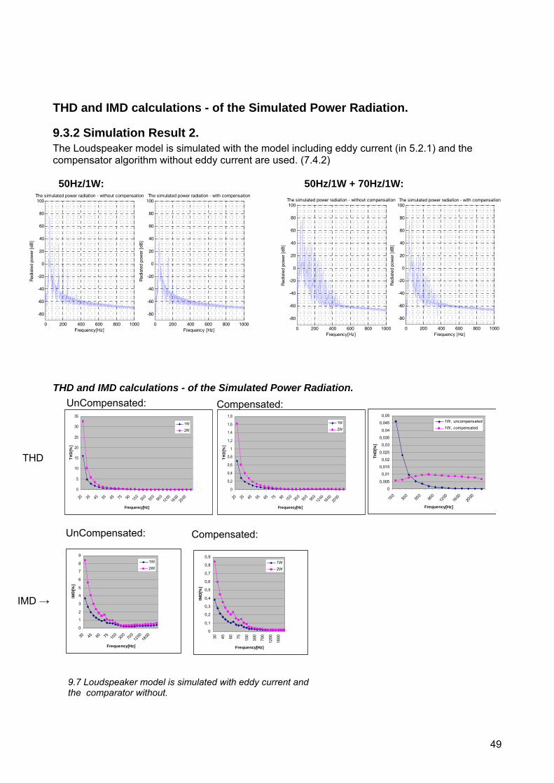
49


9.3.2 Simulation Result 2. The Loudspeaker model is simulated with the model including eddy current (in 5.2.1) and the compensator algorithm without eddy current are used. (7.4.2) 50Hz/1W: 50Hz/1W + 70Hz/1W:


THD

0

5

10

15

20

25

30

35

20 35 45 55 65 75 90 150

300

500

900

1200

1600

2000

Frequency[Hz]

THD

[%]

1W2W

0

0,2

0,4

0,6

0,8

1

1,2

1,4

1,6

1,8

20 35 45 55 65 75 90 150

300

500

900

1200

1600

2000

Frequency[Hz]

THD

[%]

1W2W

0

0,005

0,01

0,015

0,02

0,025

0,03

0,035

0,04

0,045

0,05

150

300

500

900

1200

1600

2000

Frequency[Hz]

TH

D[%

]


0

1

2

3

4

5

6

7

8

9

30 45 60 75 100

300

700

1200

1800

Frequency[Hz]

IMD

[%]

1W2W

0

0,1

0,2

0,3

0,4

0,5

0,6

0,7

0,8

0,9

30 45 60 75 100

300

700

1200

1800

Frequency[Hz]

IMD

[%]

1W2W

IMD →



0 200 400 600 800 1000

-80

-60

-40

-20

0

20

40

60

80


Rad

iate

d po

wer

[dB

]

Frequency [Hz]0 200 400 600 800 1000

-80

-60

-40

-20

0

20

40

60

80


Rad

iate

d po

wer

[dB

]

Frequency[Hz]

0 200 400 600 800 1000

-80

-60

-40

-20

0

20

40

60

80


Rad

iate

d po

wer

[dB

]

Frequency[Hz]0 200 400 600 800 1000

-80

-60

-40

-20

0

20

40

60

80


Rad

iate

d po

wer

[dB

]

Frequency [Hz]

9.7 Loudspeaker model is simulated with eddy current and the comparator without.

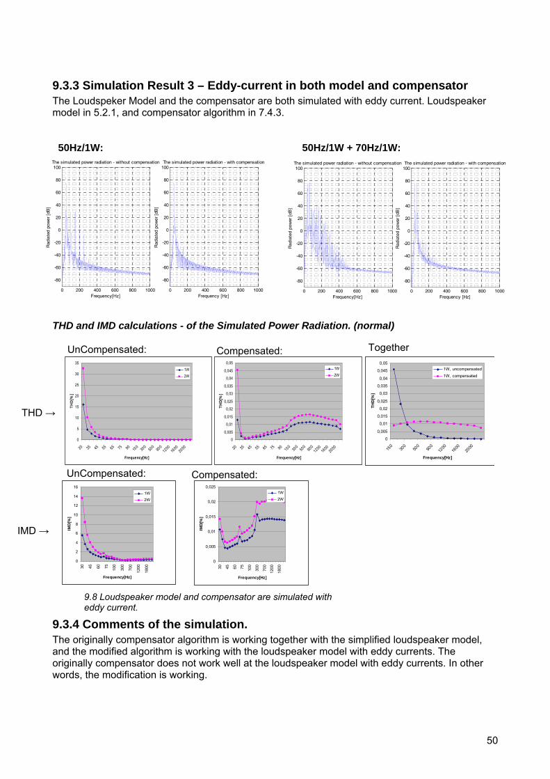
50

9.3.3 Simulation Result 3 – Eddy-current in both model and compensator The Loudspeker Model and the compensator are both simulated with eddy current. Loudspeaker model in 5.2.1, and compensator algorithm in 7.4.3. 50Hz/1W: 50Hz/1W + 70Hz/1W:

THD and IMD calculations - of the Simulated Power Radiation. (normal)

T

9.3.4 Comments of the simulation. The originally compensator algorithm is working together with the simplified loudspeaker model, and the modified algorithm is working with the loudspeaker model with eddy currents. The originally compensator does not work well at the loudspeaker model with eddy currents. In other words, the modification is working.

THD →

0

5

10

15

20

25

30

35

20 35 45 55 65 75 90 150

300

500

900

1200

1600

2000

Frequency[Hz]

THD

[%]

1W2W

0

0,005

0,01

0,015

0,02

0,025

0,03

0,035

0,04

0,045

0,05

20 35 45 55 65 75 90 150

300

500

900

1200

1600

2000

Frequency[Hz]

THD[

%]

1W2W

0

0,005

0,01

0,015

0,02

0,025

0,03

0,035

0,04

0,045

0,05

150

300

500

900

1200

1600

2000

Frequency[Hz]

THD

[%]



IMD →

0 200 400 600 800 1000

-80

-60

-40

-20

0

20

40

60

80


Rad

iate

d po

wer

[dB

]

Frequency[Hz]0 200 400 600 800 1000

-80

-60

-40

-20

0

20

40

60

80


Rad

iate

d po

wer

[dB

]

Frequency [Hz]


0

2

4

6

8

10

12

14

16

30 45 60 75 100

300

700

1200

1800

Frequency[Hz]

IMD[

%]

1W2W

0

0,005

0,01

0,015

0,02

0,025

30 45 60 75 100

300

700

1200

1800

Frequency[Hz]

IMD[

%]

1W2W

0 200 400 600 800 1000

-80

-60

-40

-20

0

20

40

60

80


Rad

iate

d po

wer

[dB

]

Frequency [Hz]0 200 400 600 800 1000

-80

-60

-40

-20

0

20

40

60

80


Rad

iate

d po

wer

[dB

]

Frequency[Hz]

Together

9.8 Loudspeaker model and compensator are simulated with eddy current.

51

The IMD is measured with f1=63Hz and f2 starts at 20Hz, and increases first in steps on five dB. Later the step increases.

9.3.5 Instability problem with the compensation algorithm If the amplitude of the excursion is excides about 8mm, the compensator gets unstable. This probably is caused by the polynomial modelling of the linear parameters. The polynomials diverge rapidly outside the measured range. (see figure 9.1)

10. DSP Programming 10.1 Overview of DSP functions void linear_model Appendix: B1 The linear model in 3.2.6. void nonlinear_model Appendix: B2 The nonlinear model in 5.2.1. void nonlinear_model_comp Appendix: B3 The nonlinear compensation algorithm in 7.4.3 + The nonlinear model in 6.3. Output: processed music signal u(n). void get_linear_parameters Appendix: B4 The linear parameter nonlinear model in 6.3. void get_nonlinear_parameters Appendix: B5 Loudspeaker B (8480277) void Gain Appendix: B6 Slow update of the Gain, or Gm in figure 12.2. The compensator becomes instable Is Gm changes to fast void Peak Appendix: B7 Peak detection void Rms Appendix: B8 Rms calculation void add_matrices_3 Appendix: B9 Adding two 3x1 matrixes void mult_matrices_3 Appendix: B10 Multiplying two 3x1 matrixes void add_matrices_4 Appendix: B11 Adding two 4x1 matrixes void mult_matrices_4 Appendix: B12 Multiplying two 4x1 matrixes

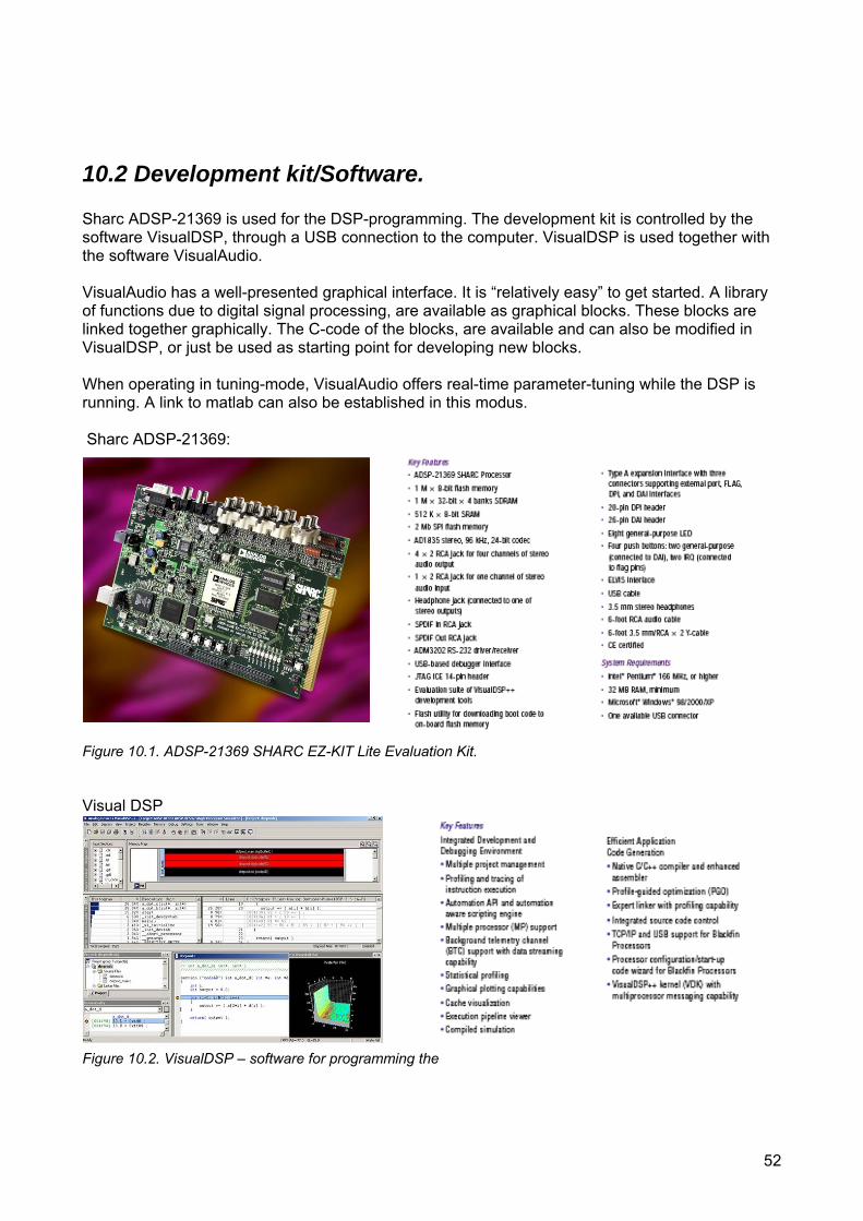
52

10.2 Development kit/Software. Sharc ADSP-21369 is used for the DSP-programming. The development kit is controlled by the software VisualDSP, through a USB connection to the computer. VisualDSP is used together with the software VisualAudio. VisualAudio has a well-presented graphical interface. It is “relatively easy” to get started. A library of functions due to digital signal processing, are available as graphical blocks. These blocks are linked together graphically. The C-code of the blocks, are available and can also be modified in VisualDSP, or just be used as starting point for developing new blocks. When operating in tuning-mode, VisualAudio offers real-time parameter-tuning while the DSP is running. A link to matlab can also be established in this modus. Sharc ADSP-21369:

Figure 10.1. ADSP-21369 SHARC EZ-KIT Lite Evaluation Kit. Visual DSP Figure 10.2. VisualDSP – software for programming the

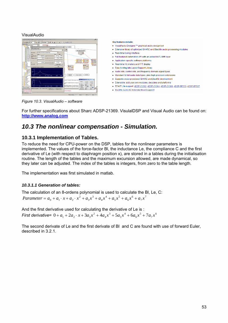
53

VisualAudio Figure 10.3. VisualAudio – software For further specifications about Sharc ADSP-21369. VisulalDSP and Visual Audio can be found on: http://www.analog.com 10.3 The nonlinear compensation - Simulation.

10.3.1 Implementation of Tables. To reduce the need for CPU-power on the DSP, tables for the nonlinear parameters is implemented. The values of the force-factor Bl, the inductance Le, the compliance C and the first derivative of Le (with respect to diaphragm position x), are stored in a tables during the initialisation routine. The length of the tables and the maximum excursion allowed, are made dynamical, so they later can be adjusted. The index of the tables is integers, from zero to the table length. The implementation was first simulated in matlab.

10.3.1.1 Generation of tables: The calculation of an 8-ordens polynomial is used to calculate the Bl, Le, C:

77

66

55

44

33

2210 xaxaxaxaxaxaxaaParameter +++++⋅+⋅+=

And the first derivative used for calculating the derivative of Le is : First derivative= 6

75

64

53

42

321 7654320 xaxaxaxaxaxaa +++++⋅++ The second derivate of Le and the first derivate of Bl and C are found with use of forward Euler, described in 3.2.1.

http://www.analog.com/

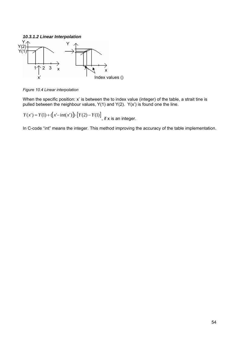
54

10.3.1.2 Linear Interpolation

Figure 10.4 Linear interpolation When the specific position: x’ is between the to index value (integer) of the table, a strait tine is pulled between the neighbour values, Y(1) and Y(2). Y(x’) is found one the line.

[ ] [ ])1()2())'int('()1()'( YYxxYxY −⋅−+=, if x is an integer.

In C-code “int” means the integer. This method improving the accuracy of the table implementation.

x x

Y Y

Index values () x’

1 2 3

Y(1) Y(2)

55

10.3.1.2 Simulating Result – Lookup table used in loudspeaker model The maximum excursion is set to ±20mm, and different length of tables are simulated in matlab to find the required table length. Matlab, Polynom Matlab, table:3200 Matlab linear rounding, table 200

0 200 400 600 800 1000

-80

-60

-40

-20

0

20

40

60

80

100The simulated power radiation - without compensatio

Rad

iate

d p

ow

er [d

B]

Frequency[Hz]0 200 400 600 800 1000

-80

-60

-40

-20

0

20

40

60

80

100The simulated power radiation - without compensatio

Rad

iate

d p

ow

er [d

B]

Frequency[Hz] 0 200 400 600 800 1000

-80

-60

-40

-20

0

20

40

60

80

100The simulated power radiation - without compensat

Rad

iate

d p

ow

er [d

B]

Frequency[Hz] Matlab rounding, table 3200 Matlab rounding, table 32000

0 200 400 600 800 1000

-80

-60

-40

-20

0

20

40

60

80


Rad

iate

d p

ow

er [d

B]

Frequency[Hz] 0 200 400 600 800 1000

-80

-60

-40

-20

0

20

40

60

80


Rad

iate

d p

ow

er [d

B]

Frequency[Hz] Figure 10.5 Comparing simulation of the loudspeaker model using different resolution in the tables for NonLinear Parameters Linear Interpolation is really improving the result for in the simulation. A table-length of 3200 is chosen. No changes compared to the polynomial simulation is seen. The table length of 3200 means a solution on:

mmm μ5.12320020

=±

step size in the table.

10.3.1.2 Simulating Result – Lookup table used in Compensator The nonlinear parameters of the loudspeaker model, is simulated with polynomials, while the nonlinear parameters of the compensator is simulated with use of lookup tables. This is done to imitate a real situation where the compensator is acting on a real loudspeaker.

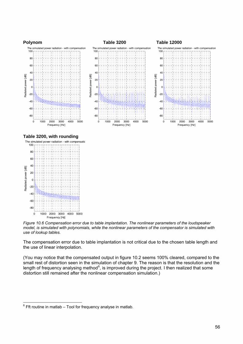
56

Polynom Table 3200 Table 12000

0 1000 2000 3000 4000 5000

-80

-60

-40

-20

0

20

40

60

80


Rad

iate

d po

wer

[dB

]

Frequency [Hz] 0 1000 2000 3000 4000 5000

-80

-60

-40

-20

0

20

40

60

80


Rad

iate

d po

wer

[dB

]

Frequency [Hz] 0 1000 2000 3000 4000 5000

-80

-60

-40

-20

0

20

40

60

80


Rad

iate

d po

wer

[dB

]

Frequency [Hz] Table 3200, with rounding

0 1000 2000 3000 4000 5000

-80

-60

-40

-20

0

20

40

60

80

100The simulated power radiation - with compensatio

Rad

iate

d p

ow

er [d

B]

Frequency [Hz] Figure 10.6 Compensation error due to table implantation. The nonlinear parameters of the loudspeaker model, is simulated with polynomials, while the nonlinear parameters of the compensator is simulated with use of lookup tables. The compensation error due to table implantation is not critical due to the chosen table length and the use of linear interpolation. (You may notice that the compensated output in figure 10.2 seems 100% cleared, compared to the small rest of distortion seen in the simulation of chapter 9. The reason is that the resolution and the length of frequency analysing method6, is improved during the project. I then realized that some distortion still remained after the nonlinear compensation simulation.)

6 Fft routine in matlab – Tool for frequency analyse in matlab.

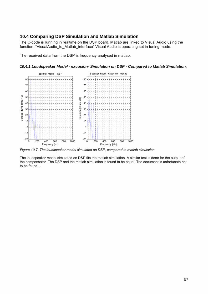
57

10.4 Comparing DSP Simulation and Matlab Simulation The C-code is running in realtime on the DSP board. Matlab are linked to Visual Audio using the function: “VisualAudio_to_Matlab_interface” Visual Audio is operating set in tuning mode. The received data from the DSP is frequency analysed in matlab.

10.4.1 Loudspeaker Model - excusion- Simulation on DSP - Compared to Matlab Simulation.

0 200 400 600 800 1000-20

-10

0

10

20

30

40

50

60

70

80

speaker model - DSP

Vol

tage

[dB

V]

(RM

S-1

V)

Frequency [Hz]0 200 400 600 800 1000

-20

-10

0

10

20

30

40

50

60

70

80

Speaker model - excusion - matlab

Exc

usio

n [r

elat

iv d

B]

Frequency [Hz]

Figure 10.7. The loudspeaker model simulated on DSP, compared to matlab simulation. The loudspeaker model simulated on DSP fits the matlab simulation. A similar test is done for the output of the compensator. The DSP and the matlab simulation is found to be equal. The document is unfortunate not to be found…

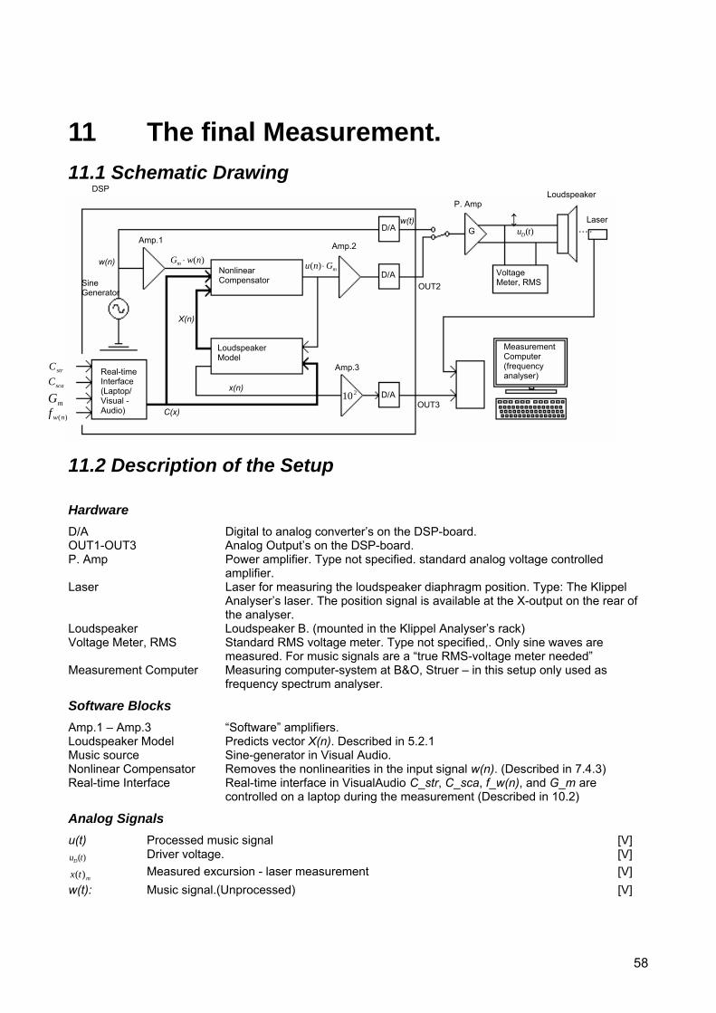
58

11 The final Measurement. 11.1 Schematic Drawing

11.2 Description of the Setup

Hardware D/A Digital to analog converter’s on the DSP-board. OUT1-OUT3 Analog Output’s on the DSP-board. P. Amp Power amplifier. Type not specified. standard analog voltage controlled

amplifier. Laser Laser for measuring the loudspeaker diaphragm position. Type: The Klippel

Analyser’s laser. The position signal is available at the X-output on the rear of the analyser.

Loudspeaker Loudspeaker B. (mounted in the Klippel Analyser’s rack) Voltage Meter, RMS Standard RMS voltage meter. Type not specified,. Only sine waves are

measured. For music signals are a “true RMS-voltage meter needed” Measurement Computer Measuring computer-system at B&O, Struer – in this setup only used as

frequency spectrum analyser.

Software Blocks Amp.1 – Amp.3 “Software” amplifiers. Loudspeaker Model Predicts vector X(n). Described in 5.2.1 Music source Sine-generator in Visual Audio. Nonlinear Compensator Removes the nonlinearities in the input signal w(n). (Described in 7.4.3) Real-time Interface Real-time interface in VisualAudio C_str, C_sca, f_w(n), and G_m are

controlled on a laptop during the measurement (Described in 10.2)

Analog Signals u(t) Processed music signal [V]

)(tuD Driver voltage. [V]

mtx )( Measured excursion - laser measurement [V] w(t): Music signal.(Unprocessed) [V]

OUT1

mG

mG1 u(n)

u(t)

mtx )(

DSP

C(x) OUT3

D/A

Amp.3

x(n)

Real-time Interface (Laptop/ Visual -Audio)

strC

scaC

mG

)(nwf


Loudspeaker Model

D/A

Measurement Computer (frequency analyser)

OUT2

X(n)

Sine Generator

P. Amp

Laser

Voltage Meter, RMS

D/A

Amp.1 Amp.2

w(n)

G

210

)(tuD

Loudspeaker

w(t)

)(nwGm ⋅ mGnu ⋅)(

59

Discrete, digital signals C(x) Compliance – function of position, x(n)). [m/N] u (n) Processed music signal. [V] w(n) Music signal. [V] x(n) Diaphragm position [m] X(n) Predicted state vector (one sample into the future). Consists of current, Lei ,

eddy current, Lei , voice-coil position x (n) - and velocity, )(nv .

Manually controlled Parameters (real time tuning with laptop/VisualAudio)

)(nwf The frequency of the sine-wave, w(n).

mG Internal gain. – measurement of the power amplifier gain, G.

scaC Scaling factor for the compliance curve. (Described in XXXi)

strC Stretch factor for the x-axel for the compliance curve. (Described in XXXi)

Others symbols G The gain of the power amplifier

Setup Description An internal sine-generator in Visual Audio generates music source, w(n). The frequency of w(n), f_w(n), is available for real time tuning in VisualAudio. After the D/A converter w(n) becomes w(t) and is set to OUT.1 on the DSP board. Amp.1 fits the amplitude of w(n) to the level where the loudspeaker is operating. G_m is manually set to equal the gain of the external power amplifier(G), (the voltmeter is used) . Amp.2 reintroduces the original level to u(n). u(n) is D/A-converted and set to OUT.2. The level of the predicted diaphragm position, x(n) is multiplied by 100 (in Amp3), to get a decent signal to noise level for the measurement. Update functionality of the linear parameters and current/voltage measurements are not implemented in the final setup. C_str, C_sca, f_w(n), and G_m are manually controlled during the measurement. The DSP board are connected to a laptop, and the parameters are available for real time tuning, in VisualAudio’s. When the parameters are tuned in realtime, the DSP program adjusted the parameters little by little, until the wanted state is achieved. If the parameters changes too fast, the compensator algorithm gets instable.

60

11.3 Measurement result. In figure 11.1 and 11.2 are the measurement results for 50Hz and 70Hz sine waves at 1W. On top are the loudspeaker outputs without compensation (excursion measurement, laser. OUT1 on the DSP board are connected to the power amp). In the middle are the predicted excursions from the loudspeaker model (measured at OUT3), and lowest are the loudspeaker outputs with compensation (excursion measurement, laser. OUT1 on the DSP board are connected to the power amp). The measured values are relative decibel values. The absolute excursion values are not identified. The excursion signal from the loudspeaker model (OUT3, seen in figure X, c&d) is simply scaled to fit the magnitude of the loudspeaker measurement, by tuning the gain of Amp.3. (the fundamentals are scaled to roughly equal).

net-power infection The net-power infects the measurement, as seen in figure 11.1b. The 50Hz component is seen about 30 dB below the 70Hz signal. Due to intermodulation occurs also a 20Hz component. In figure 11.1d is the third harmonic of the net power detected. The magnitude of the net-power infection are small, anyway the problem would is avoided by using another frequency than 50Hz.

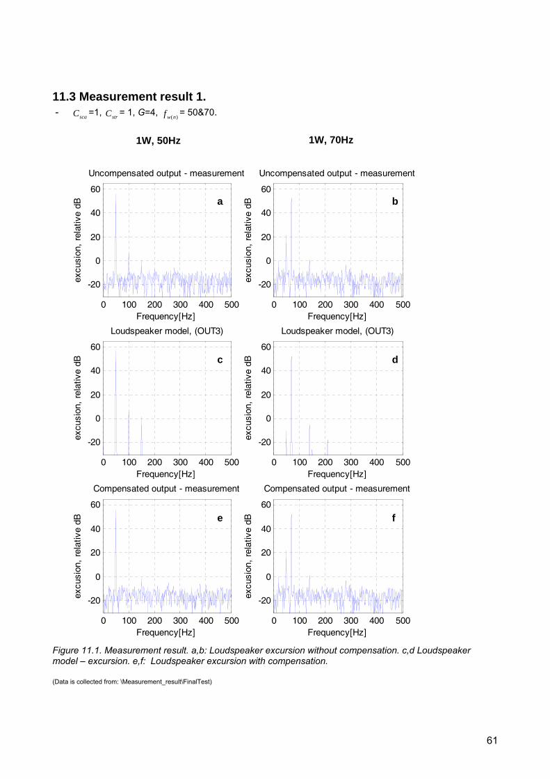
61

11.3 Measurement result 1. - scaC =1, strC = 1, G=4, )(nwf = 50&70.

0 100 200 300 400 500

-20

0

20

40

60

Frequency[Hz]

excu

sion

, re

lativ

e dB

Uncompensated output - measurement

0 100 200 300 400 500

-20

0

20

40

60

Frequency[Hz]

excu

sion

, re

lativ

e dB


0 100 200 300 400 500

-20

0

20

40

60

Frequency[Hz]

excu

sion

, re

lativ

e dB


0 100 200 300 400 500

-20

0

20

40

60

Frequency[Hz]

excu

sion

, re

lativ

e dB


0 100 200 300 400 500

-20

0

20

40

60

Frequency[Hz]

excu

sion

, re

lativ

e dB

Compensated output - measurement

0 100 200 300 400 500

-20

0

20

40

60

Frequency[Hz]

excu

sion

, re

lativ

e dB


Figure 11.1. Measurement result. a,b: Loudspeaker excursion without compensation. c,d Loudspeaker model – excursion. e,f: Loudspeaker excursion with compensation. (Data is collected from: \Measurement_result\FinalTest)

1W, 50Hz 1W, 70Hz

a b

c d

e f

62

1W - 50Hz The nonlinear compensation is somehow successful for the 50Hz input signal. In the compensated output the second harmonic (100Hz) is removed, while the third harmonic is decreased by 1.6 dB. As seen in the figure X,c&d does the loudspeaker model fit the loudspeaker pretty well. “Absolute values” 50Hz, 1W Fundamental 2. harmonic 3.harmonicUncompensated output 56,2 5,9 0,7Loudspeaker model 57 5,9 1,5Compensated output 56,1 - -1(Data is collected from: \Measurement_result\FinalTest) Relative values (the fundamental is scaled to 0 dB)


1W -70Hz For the 70Hz input signal the compensation does not work at all. The harmonics remains unchanged after the compensation. The loudspeaker model does not fit the loudspeaker. The harmonics are underestimated in the loudspeaker model. Absolute values

(Data is collected from: \Measurement_result\FinalTest) Relative values (the fundamental is scaled to 0 dB)

Data is collected from: \Measurement_result\FinalTest)

50Hz, 1W Fundamental 2. harmonic 3.harmonicUncompensated output 0 -50.3 -55.5Loudspeaker model 0 -51.1 -55,5Compensated output 0 - -57.1

70Hz, 1W Fundamental 2. harmonic 4.harmonicUncompensated output 52,7 0,8 3.3Loudspeaker model 52,6 -5,2 -Compensated output 52,7 0,8 -3.3

70Hz, 1W Fundamental 2. harmonic 4.harmonicUncompensated output 0 -51.9 -56Loudspeaker model 0 -57.8 -Compensated output 0 -51.9 -56

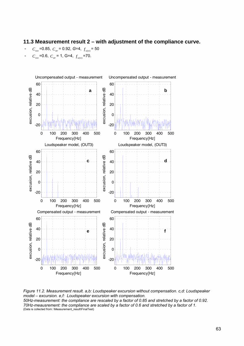
63

11.3 Measurement result 2 – with adjustment of the compliance curve. - scaC =0.85, strC = 0.92, G=4, )(nwf = 50 - scaC =0.6, strC = 1, G=4, )(nwf =70.

Figure 11.2. Measurement result. a,b: Loudspeaker excursion without compensation. c,d: Loudspeaker model – excursion. e,f: Loudspeaker excursion with compensation. 50Hz-measurement: the compliance are rescaled by a factor of 0.85 and stretched by a factor of 0.92. 70Hz-meausrement: the compliance are scaled by a factor of 0.6 and stretched by a factor of 1. (Data is collected from: \Measurement_result\FinalTest)

0 100 200 300 400 500

-20

0

20

40

60

Frequency[Hz]

excu

sion

, re

lativ

e dB


0 100 200 300 400 500

-20

0

20

40

60

Frequency[Hz]

excu

sion

, re

lativ

e dB


0 100 200 300 400 500

-20

0

20

40

60

Frequency[Hz]

excu

sion

, re

lativ

e dB


0 100 200 300 400 500

-20

0

20

40

60

Frequency[Hz]

excu

sion

, re

lativ

e dB


0 100 200 300 400 500

-20

0

20

40

60

Frequency[Hz]

excu

sion

, re

lativ

e dB


0 100 200 300 400 500

-20

0

20

40

60

Frequency[Hz]

excu

sion

, re

lativ

e dB


a b

c d

e f

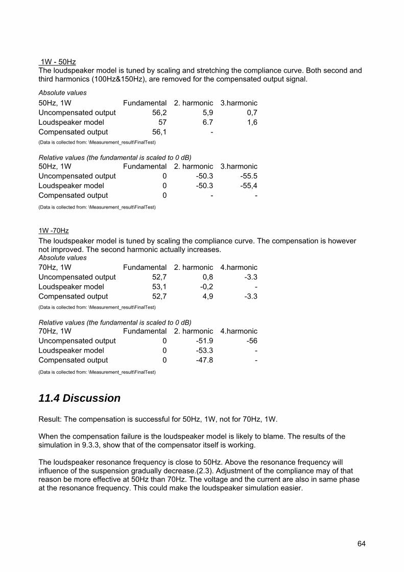
64

1W - 50Hz The loudspeaker model is tuned by scaling and stretching the compliance curve. Both second and third harmonics (100Hz&150Hz), are removed for the compensated output signal. Absolute values




1W -70Hz The loudspeaker model is tuned by scaling the compliance curve. The compensation is however not improved. The second harmonic actually increases. Absolute values




11.4 Discussion Result: The compensation is successful for 50Hz, 1W, not for 70Hz, 1W. When the compensation failure is the loudspeaker model is likely to blame. The results of the simulation in 9.3.3, show that of the compensator itself is working. The loudspeaker resonance frequency is close to 50Hz. Above the resonance frequency will influence of the suspension gradually decrease.(2.3). Adjustment of the compliance may of that reason be more effective at 50Hz than 70Hz. The voltage and the current are also in same phase at the resonance frequency. This could make the loudspeaker simulation easier.

50Hz, 1W Fundamental 2. harmonic 3.harmonicUncompensated output 56,2 5,9 0,7Loudspeaker model 57 6.7 1,6Compensated output 56,1 -

50Hz, 1W Fundamental 2. harmonic 3.harmonicUncompensated output 0 -50.3 -55.5Loudspeaker model 0 -50.3 -55,4Compensated output 0 - -

70Hz, 1W Fundamental 2. harmonic 4.harmonicUncompensated output 52,7 0,8 -3.3Loudspeaker model 53,1 -0,2 -Compensated output 52,7 4,9 -3.3

70Hz, 1W Fundamental 2. harmonic 4.harmonicUncompensated output 0 -51.9 -56Loudspeaker model 0 -53.3 -Compensated output 0 -47.8 -

65

The loudspeaker model is tuned to fit the loudspeaker, by compliance adjustment, and the adjustment is based on frequency analyses. Apparently the tuning seems successful for both frequencies. The frequency contents of the loudspeaker model and loudspeaker are equalized. Signals with equal frequency spectrum do not necessary look the same in time domain. Tuning of the loudspeaker model by just looking into the frequency domain, may not be satisfactory. The klippel analyser is way more complex than this simple manually suspension tuning procedure, but anyway the principle is the same. As described in 8.1.1, do the analyser use a nonlinear loudspeaker model and extracts the parameters by applying different test signals. But several setting of the nonlinear parameters can give the same output, for a specific test signal. As shown in figure 8.1.2.1, do the analyser in some cases failure. This result is measured with the old software.

66

12. The Future Setup 12.1 Schematic Drawing – The adaptive system

12.2 Description

Hardware A/D Analog to Digital converter’s on the DSP-board. D/A Digital to analog converter’s on the DSP-board. Feedback network Feedback network. Adapts the driver voltage from ±55V to ±1.5V. IN1,IN2,IN3 Analog input’s on DPS-board.(max voltage: ±1.5V) Music source CD player or similar music source. OUT1 Analog Output on the DSP-board. P. Amp Power amplifier. Type not specified. standard analog voltage controlled

amplifier. Rs Shunt resistor, due to the current measurement (high power resistor)

Software Blocks Amp.1 – Amp.3 “Software” amplifiers. Loudspeaker Model Predicts vector X(n). Described in 5.2.1 Nonlinear Compensator Removes the nonlinearities in the input signal w(n). (Described in 7.4.3) Parameter Identifier Updates linear parameters, in vector K. (Not described in detail, see 1.1) zx The time delay of the D/A converter and the power amplifier. (synchronizing the

measured and simulated current)

Rs

Ra

Rb Rc

Rd

A/D

A/D

zx

mG OUT1

Amp.1

Amp.3

u(n)

Amp.4

fbG2

u(t) G

mGnu ⋅)(Nonlinear Compensator

Loudspeaker Model

Parameter Indentifier

A/D D/A

mG

mLei Lei

X(n)

K(n) + C(x)

P. Amp Loudspeaker

DSP

IN1

Music source

Amp.2 w(n) w(t)

)()(

nunu mD

mG1)(nwGm ⋅

)(tuD

u(n-zx)

IN2

(IN3)

fbG

fbG

Feedback network 1

Feedback network 2

fbG2

2)(tuD

2)(tu RSD+

2)( fbRSD Gtu ⋅+

mD nu )(

mRSD nu )(+

)(tu RSD+

2)( fbD Gtu ⋅

s

mDmRSD

Rnunu

⋅−+

2)()(

67

Analog signals u (t): Processed music signal. [V]

)(tuD Driver voltage. [V] )(tu RSD+ Driver voltage + the voltage drop of Rs. [V]

w(t): Music signal.(Unprocessed) [V]

Discrete, digital signals C(x) Compliance – function of position, x(n). [m/N]

Lei Voice-coil current - Predicted value by loudspeaker model A]

mLei Voice-coil current – measured value. [A] K(n) Vector consisting the linear parameter.

)(nu Processed music signal. [V]

mD nu )( Driver voltage – measured value. [V]

mRSD nu )(+ Driver voltage + the voltage drop of Rs - measured value. [V]

w(n): Music signal. [V] u (n): Processed music-signal. [V] X(n): Predicted state vector (one sample into the future). Consists of current, Lei ,

eddy current, Lei , voice-coil position x (n) - and velocity, )(nv .

Others symbols G The gain of the external power amplifier (P.Amp).

mG Internal gain. – Measurement of the power amplifier’s gain, G

fbG Gain of the feedback network for driver voltage measurements. ( )(tuD)

Description of the Setup In the future setup is the update functionality of the linear parameters and current/voltage measurements implemented. An external source, for instance a CD-player, is generating the music-signal, w(n). Amp.1 fits the amplitude of w(n) to the level where the loudspeaker is operating. Amp.2 reintroduces the original level to u(n). The internal gain, G_m, is automatically adjusted to equal the gain of the external power amplifier, G. Rms values of u and u_D sho

)()(

nunuG mD

m =

Rms values of u and u_D should be used. Gm must not be updated to fast. The compensator could be instable. The block “Parameter Identification” updates the linear parameters and the compliance curve, based one the current measurement. The functionality is not described in this thesis.

The measured voice-coil current, mLeis

mDmRSDmLe R

nunui⋅−

= +

2)()(

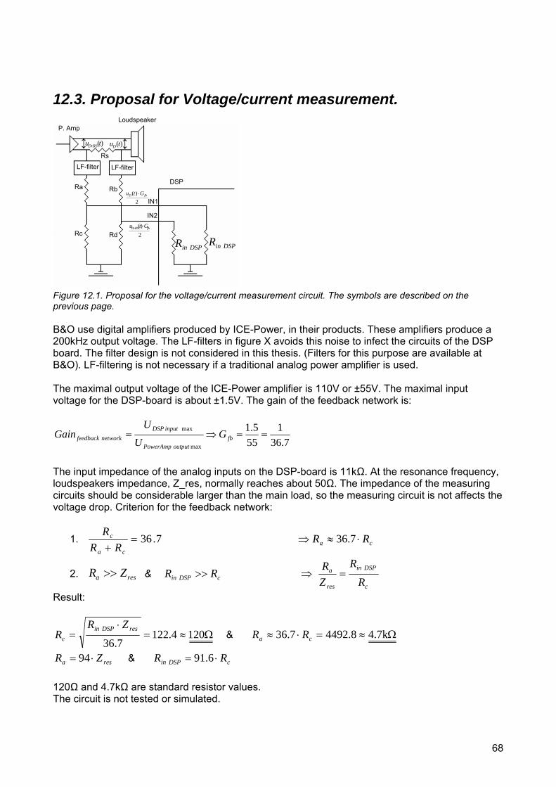
68

12.3. Proposal for Voltage/current measurement. 6. Conclusion.

Figure 12.1. Proposal for the voltage/current measurement circuit. The symbols are described on the previous page. B&O use digital amplifiers produced by ICE-Power, in their products. These amplifiers produce a 200kHz output voltage. The LF-filters in figure X avoids this noise to infect the circuits of the DSP board. The filter design is not considered in this thesis. (Filters for this purpose are available at B&O). LF-filtering is not necessary if a traditional analog power amplifier is used. The maximal output voltage of the ICE-Power amplifier is 110V or ±55V. The maximal input voltage for the DSP-board is about ±1.5V. The gain of the feedback network is:

7.361

555.1

max

max==⇒= fb

outputPowerAmp

inputDSPnetworkfeedback G

U

UGain

The input impedance of the analog inputs on the DSP-board is 11kΩ. At the resonance frequency, loudspeakers impedance, Z_res, normally reaches about 50Ω. The impedance of the measuring circuits should be considerable larger than the main load, so the measuring circuit is not affects the voltage drop. Criterion for the feedback network:

1. 7.36=+ ca

c

RRR

ca RR ⋅≈⇒ 7.36

2. resa ZR >> & cDSPin RR >> ⇒ c

DSPin

res

a

R

R

ZR

=

Result:

Ω≈=⋅

= 120122.47.36

resDSPinc

ZRR & Ω≈=⋅≈ 4.7k4492.87.36 ca RR

resa ZR ⋅= 94 & cDSPin RR ⋅= 6.91 120Ω and 4.7kΩ are standard resistor values. The circuit is not tested or simulated.

Loudspeaker

Ra Rb

Rc

DSPinR

DSP

IN1

IN2

P. Amp

LF-filter LF-filter

Rd

DSPinR

Rs

2)( fbRSD Gtu ⋅+

2)( fbD Gtu ⋅

)(tuD )(tu RSD+

69

13. Conclusion. Compensation of loudspeaker nonlinearities is investigated. A compensation system based on a loudspeaker model (a computer model/simulation of the real loudspeaker), is implemented on DSP. The system is briefly tested for pure tones, and the loudspeaker diaphragm excursion is used as output measure. The loudspeaker parameters are measured with the Klippel Analyser, a tool for loudspeaker parameter detection. Based on these results are the loudspeaker modelled in matlab, and the result is briefly compared to the real loudspeaker. Adjustments of the compliance of the suspension, is used to improve the result. The “feedback linearization” algorithm in [Schurer, Slump and Herrmann, 1998] is chosen as the nonlinear compensation-algorithm. It is slightly modified to fit the loudspeaker model used in this thesis. Originally it is designed for a simpler loudspeaker model, not including eddy currents. The result is satisfying. The nonlinear distortion is as good as eliminated in the simulation. Due to temperature and aging the loudspeaker parameters are drifting. In previous investigations, like [Bright, 2002] it is found that the drifting mainly is located in the loudspeakers linear parameters. The loudspeaker model therefore needs an online tracking system (known as parameter identification), which continuously update the linear parameters. Previous investigations, and also measurements done in this thesis, show that nonlinear drifting in the compliance of the suspension also must be taken in account, at least for a traditionally hi-fi-loudspeaker. There was not time enough for looking into parameter identification. Without the parameter identification, the compensation system is briefly tested in a simplified setup. The loudspeaker model is manually adjusted to fit the real loudspeaker. The compliance is tuned by realtime stretching and scaling functionality implemented on DSP. The system seems to work for some input frequencies and do not work for others. This is further described in 11.4. To carry out an adaptive system, able to handle the loudspeaker drifting due to temperature and aging, is a subject for further investigation.

70

14. References. [Agerkvist, 2007] Agerkvist, Finn t. (Sept. 2007) “Modellin Loudspeaker Non-Linearities”. AES 32nd International Conference, Hillerød, Denmark, [Andersen, 2005] Andersen, Martin Rune. ”Compensation of Nonlinearities in Transducers” [Bright, 2002] Bright, A. (2002). Active Control of Loudspeakers: An Investigation of Practical Applications. PhD thesis, The Technical University of Denmark, Department of Acoustic Technology - Ørsted·DTU. [Klippel, 1992] Klippel, W. (1992). “The mirror filter - a new basis for reducing nonlinear distortion and equalizing response in woofer systems.” J. Audio Eng. Soc., Vol. 40(No. 9):pp. 675–691. [Klippel, 1998,a] Klippel, W. (1998). “Direct feedback linearization of nonlinear loudspeaker systems”. J. Audio Eng. Soc., Vol. 46(No. 6):pp. 499–507. [Klippel, 1998,b] Klippel, W. (1998). “Adaptive Nonlinear Control of Loudspeaker Systems”. Audio Eng. Soc., Vol. 46, No. 11. [Klippel, 1998,c] Klippel, W. (1998). “Nonlinear Adaptive Controller for Loudspeakers with Current Sensor” [Klippel, 2003] Klippel,W. “Nonlinear modeling of heat transfer in loudspeakers”. Audio Eng Soc, 114th Convention. [Knudsen & Jensen, 1993] M. H. Knudsen, and J. G. Jensen. “Low-frequency loudspeaker models that include suspension creep”. J. Audio Eng. Soc., Vol. 41, No. 1 / 2, 1993 [Krump, 1997] Krump, G. (1997): Zur Temperaturabhängigkeit von Lautsprecherparametern, presented at DAGA-97. ISBN 3-9804568-2-X [Leach, 1999] Leach, W. M. (1999). “Introduction to Electroacoustics and Audio Amplifier Design”. Kendall/Hunt Publiching Company, 3. edition. [Pedersen, 2007] Pedersen, Bo Rohde. (Sept. 2007) “Musical transducer-less identification of linear loudspeaker parameters”. AES 32nd International Conference, Hillerød, Denmark, [Pedersen and Rubak, 2007] Pedersen, Bo. R. and Rubak Per (2007) “Online Identification of Linear Loudspeaker Parameters”, AES 122nd Vienna, Austria [Schurer, Slump and Herrmann, 1998] Schurer, Hans, Cornelis H. Slump, and Otto E. Herrmann, (Sept. 1998) “Theoretical and Experimental Comparison of Three Methods for Compensation of Electrodynamic Transducer Nonlinearity”. Journal of theAudio Eng. Soc., 46, pp. 723– 740. [Thiele, 1961] Thiele, A. N. (1961). Loudspeakers in vented boxes. Proceedings of the IRE Australia;”reprinted in J. Audio Eng. Soc., 19: pp. 382-392 (May 1971)”, Vol. 22:pp. 487–508.

71

Appendix A Matlab Code A1. linear_Loudspeaker_Model_Simplified function [X ] = linear_Loudspeaker_Model_Simplified(u,a,b,c,M,Re,Rt,fs); %linear modelling %X(n)=state vector %Bl=force factor vector %C=total compliance vector %M=total inductance vector %R=Electrical resistance %fs=sampling rate Bl = b(1); Le = a(1)*0.001; C = c(1)*0.001; Ts=1/fs; %X=[i(n) ; x(n) ; 1/Ts*(x(]; F=[(1-((Re/Le)*Ts)) 0 (-Ts*Bl/Le); 0 1 Ts; (Ts*Bl/M) (-Ts/(C*M)) (1-Rt*Ts/M)]; G=[Ts/Le ; 0 ; 0]; X=zeros(3,length(u)); X(:,1)= [ 0 0 0 ]; for k=1:(length(u)) X(:,k+1) = F*X(:,k) + G*u(k); end end

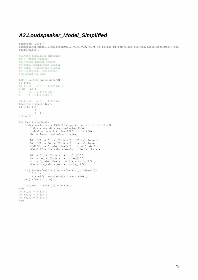
72

A2.Loudspeaker_Model_Simplified function [OUT] = Loudspeaker_Model_Simplified(w,L2_0,R2_0,M,Re,Rt,fs,Le_tab,Bl_tab,C_tab,dLe_tab,table_size,max_x,stepsize_table); %linear modelling exercise %X(n)=state vector %Bl=force factor vector %C=total compliance vector %M=total inductance vector %R=Electrical resistance %fs=sampling rate Le0 = Le_tab(table_size/2); Ts=1/fs; %X=[i(n) ; x(n) ; 1/Ts*(x(]; % Bl = b(1); % Le = a(1)*0.001; % C = c(1)*0.001; %X=[i(n) ; x(n) ; 1/Ts*(x(]; X=zeros(3,length(w)); X(:,1)= [ 0 0 0 ]; str = 1; for k=1:(length(w)) index_realvalue = X(2,k)/stepsize_table + table_size/2; index = round(index_realvalue-0.5); index2 = round( (index-1600).*str+1600); dx = index_realvalue - index; Bl_diff = Bl_tab(index+1) - Bl_tab(index); Le_diff = Le_tab(index+1) - Le_tab(index); C_diff = C_tab(index2+1) - C_tab(index2); dLe_diff = dLe_tab(index+1) - dLe_tab(index); Bl = Bl_tab(index) + dx*Bl_diff; Le = Le_tab(index) + dx*Le_diff; C = C_tab(index2) + (dx*str)*C_diff ; dLe = dLe_tab(index) + dx*dLe_diff; F=[(1-((Re/Le)*Ts)) 0 -Ts/Le*(X(1,k)*dLe+Bl); 0 1 Ts; (Ts*Bl/M) (-Ts/(C*M)) (1-Rt*Ts/M)]; G=[Ts/Le ; 0 ; 0]; X(:,k+1) = F*X(:,k) + G*w(k); end OUT(1,:) = X(1,:); OUT(3,:) = X(2,:); OUT(4,:) = X(3,:); end

73

A3. Loudspeaker_Model function [X ] = Loudspeaker_Model(u,L2_0,R2_0,M,Re,Rt,fs,Le_tab,Bl_tab,C_tab,dLe_tab,table_size,max_x,stepsize_table); %Nonlinear modelling exercise %X(n)=state vector %Bl=force factor vector %c=total compliance vector %b-total Bl vector %M=total mass %Re=Electrical resistance %Rt=Mechanical resistance %R2=electrical resistance due the eddy current losses %fs=sampling rate %unused output S1 S2 S3 S4 S5 S6 S7 str = 1; Ts=1/fs; Le0 = Le_tab(table_size/2); % converting to Henry X=zeros(4,length(u)); X(:,1)= [ 0 0 0 0 ]; % simulation loop for k=1:64000%(length(u)) % x2 = round(x1*round(tabel_size/20)+round(tabel_size/2))+1;%adding one since tabel starts at 1 (not zero) % index = round(X(3,k)/stepsize_table + table_size/2 + 0.5); index_realvalue = X(3,k)/stepsize_table + table_size/2; index = round(index_realvalue-0.5); index2 = round( (index-1600).*str+1600); dx = index_realvalue - index; Bl_diff = Bl_tab(index+1) - Bl_tab(index); Le_diff = Le_tab(index+1) - Le_tab(index); C_diff = C_tab(index2+1) - C_tab(index2); dLe_diff = dLe_tab(index+1) - dLe_tab(index); Bl = Bl_tab(index) + dx*Bl_diff; Le = Le_tab(index) + dx*Le_diff; C = C_tab(index2) + (dx*str)*C_diff ; dLe = dLe_tab(index) + dx*dLe_diff; L2 = Le*L2_0/Le0; R2 = Le*R2_0/Le0; dL2 = dLe*L2_0/Le0; %calculation of F and G matrix values F = [ 1-(Re+R2)/Le*Ts R2/Le*Ts 0 -Ts/Le*(X(1,k)*dLe+Bl); R2*Ts/L2 1-(R2*Ts/L2) 0 -Ts/L2*X(2,k)*dL2; 0 0 1 Ts ; (Ts*Bl/M) 0 (-Ts/(C*M)) (1-Rt*Ts/M) ]; G = [Ts/Le ; 0 ; 0; 0]; %calculating the state variables X(:,k+1) = F*X(:,k) + G*u(k); end end

74

A4. Nonlinear_Compensator_Simplified function [OUT,u] = Nonlinear_Compensator_Simplified(w,Le_tab,Bl_tab,C_tab, dLe_tab,L2_0,R2_0,M,Re,Rm,fs,table_size,max_x,stepsize_table); %Linear Feedback compensator (w,a,b,c,Le,Bl,C,L2_0,R2_0,M,Re,Rt,fs); % u - compensated output voltage % w - input voltage % Bl_tab - force factor vector, tabel in mm, +-10mm % Le_tab - inductance vector, tabel in mm, +-10mm % C_tab - compliense vector, tabel in mm, +-10mm % a - inductance polynomes, vector % c - compliance polynomes, vector % b - force factor polynomes, vector % M - total mass % Re - Electrical resistance % Rm - Mechanical resistance % R2 - electrical resistance due the eddy current losses % fs - sampling rate Ts = 1/fs; % Stepsize Le_0 = Le_tab(table_size/2); % inductance, converting to Henry Bl_0 = Bl_tab(table_size/2); % force factor C_0 = C_tab(table_size/2); % compliance, converting to m/N K_0 = 1/C_0; % stiffness N/m fase = 0; v = zeros(1,length(w)); % LD(linear dynamics) output vector u = zeros(1,length(w)); % compensator output vector X = zeros(3,length(w)); % X-vector for k=1:fase+1 X(:,k)= [ 0 % x1 - current 0 % x3 - excution 0 ]; % x4 - velosity end for k=1:64000 %Loading nonlinear parameters from tables index_realvalue = X(2,k)/stepsize_table + table_size/2; index = round(index_realvalue-0.5); dx = index_realvalue - index; Bl_diff = Bl_tab(index+1) - (Bl_tab(index)); Le_diff = Le_tab(index+1) - (Le_tab(index)); C_diff = C_tab(index+1) - (C_tab(index)); K_diff = 1/C_tab(index+1) - 1/C_tab(index); dLe_diff = dLe_tab(index+1) - (dLe_tab(index)); Bl = Bl_tab(index) + dx*Bl_diff; Le = Le_tab(index) + dx*Le_diff; C = C_tab(index) + dx*C_diff; K = 1/C_tab(index) + dx*K_diff; dLe = dLe_tab(index) + dx*dLe_diff; dBl = Bl_diff/stepsize_table; ddLe = dLe_diff/stepsize_table; dK = K_diff/stepsize_table; %constants for speaker model L2 = Le*L2_0/Le_0; R2 = Le*R2_0/Le_0; dL2 = dLe*L2_0/Le_0; %compensator u(k) = Le/(Bl+dLe*X(1,k))*(X(3,k)*(X(2,k)*dK + (K-K_0) - dBl*X(1,k) ... - ddLe*X(1,k)^2/2 - Bl_0^2/Le_0) + Re*X(2,k)*(K-K_0)/Le_0 - ... Re*X(1,k)*(2*Bl+dLe*X(1,k))/(2*Le_0) + Bl_0*w(k)/Le_0) + Re*X(1,k) + ... Bl*X(3,k) + dLe*X(1,k)*X(3,k);% + R2*(X(1,k)-X(2,k)); % u(k) =w(k);

75

%calculation of F and G matrix values F=[(1-((Re/Le)*Ts)) 0 -Ts/Le*(X(1,k)*dLe+Bl); 0 1 Ts; (Ts*Bl/M) (-Ts/(C*M)) (1-Rm*Ts/M)]; G=[Ts/Le ; 0 ; 0]; %calculating the state variables X(:,k+1) = F*X(:,k) + G*u(k); end OUT(1,:) = X(1,:); OUT(3,:) = X(2,:); OUT(4,:) = X(3,:); end

76

A5. Nonlinear_Compensator function [X,u] = Nonlinear_Compensator(w,Le_tab,Bl_tab,C_tab, dLe_tab,L2_0,R2_0,M,Re,Rm,fs,table_size,max_x,stepsize_table); %Linear Feedback compensator (w,a,b,c,Le,Bl,C,L2_0,R2_0,M,Re,Rt,fs); % u - compensated output voltage % w - input voltage % Bl_tab - force factor vector, tabel in mm, +-10mm % Le_tab - inductance vector, tabel in mm, +-10mm % C_tab - compliense vector, tabel in mm, +-10mm % a - inductance polynomes, vector % c - compliance polynomes, vector % b - force factor polynomes, vector % M - total mass % Re - Electrical resistance % Rm - Mechanical resistance % R2 - electrical resistance due the eddy current losses % fs - sampling rate %Units for loudspeaker model % Re[?] % Rm[kg/s] / [N*s/m] % mt[kg]!! % Le0[H]!! % Blo[N/A] % Ko[N/m] %constants (first polynom is DC-value) Ts = 1/fs; % Stepsize Le_0 = Le_tab(table_size/2); % inductance, converting to Henry Bl_0 = Bl_tab(table_size/2); % force factor C_0 = C_tab(table_size/2); % compliance, converting to m/N K_0 = 1/C_0; % stiffness N/m fase = 0; v = zeros(1,length(w)); % LD(linear dynamics) output vector u = zeros(1,length(w)); % compensator output vector X = zeros(4,length(w)); % X-vector for k=1:fase+1 X(:,k)= [ 0 % x1 - current 0 % x4 - eddy current 0 % x3 - excution 0 ]; % x4 - velosity end %k=100 %X(3,k)=0.0021 %max_x = max_excursion; for k=1:64000 %Loading nonlinear parameters from tables index_realvalue = X(3,k)/stepsize_table + table_size/2; index = round(index_realvalue-0.5); dx = index_realvalue - index; Bl_diff = Bl_tab(index+1) - (Bl_tab(index)); Le_diff = Le_tab(index+1) - (Le_tab(index)); C_diff = C_tab(index+1) - (C_tab(index)); K_diff = 1/C_tab(index+1) - 1/C_tab(index); dLe_diff = dLe_tab(index+1) - (dLe_tab(index)); Bl = Bl_tab(index) + dx*Bl_diff; Le = Le_tab(index) + dx*Le_diff; C = C_tab(index) + dx*C_diff; K = 1/C_tab(index) + dx*K_diff; dLe = dLe_tab(index) + dx*dLe_diff; dBl = Bl_diff/stepsize_table; ddLe = dLe_diff/stepsize_table; dK = K_diff/stepsize_table;

77

%constants for speaker model L2 = Le*L2_0/Le_0; R2 = Le*R2_0/Le_0; dL2 = dLe*L2_0/Le_0; %compensator u(k) = Le/(Bl+dLe*X(1,k))*(X(4,k)*(X(3,k)*dK + (K-K_0) - dBl*X(1,k) ... - ddLe*X(1,k)^2/2 - Bl_0^2/Le_0) + Re*X(3,k)*(K-K_0)/Le_0 - ... Re*X(1,k)*(2*Bl+dLe*X(1,k))/(2*Le_0) + Bl_0*w(k)/Le_0) + Re*X(1,k) + ... Bl*X(4,k) + dLe*X(1,k)*X(4,k);% + R2*(X(1,k)-X(2,k)); %calculation of F and G matrix values F = [ 1-(Re+R2)/Le*Ts R2/Le*Ts 0 -Ts/Le*(X(1,k)*dLe+Bl); R2*Ts/L2 1-(R2*Ts/L2) 0 -Ts/L2*X(2,k)*dL2; 0 0 1 Ts ; (Ts*Bl/M) 0 (-Ts/(C*M)) (1-Rm*Ts/M) ]; G = [Ts/Le ; 0 ; 0; 0]; %calculating the state variables X(:,k+1+fase) = F*X(:,k) + G*u(k); end end

78

A6 compliance_Adjustment function [X,str]= compliance_Adjustment(C,stepsize_table,table_size); x = -0.020:stepsize_table:0.020; X = 0.002; %scaling sca = 1; %Scaling-Gain C_tuned = C * sca; %stretching str = 0.8; %Stretching-Gain %smuding, model becomes unstabil if smud_factor = 10; C_mid = (smud_factor*C + C_tuned)/(smud_factor+1); %index rutine index_realvalue = x/stepsize_table + table_size/2; index = round(index_realvalue-0.5); index2 = round((index-1600).*str+1600); figure(50) plot(index,C) axis([0 3200 0 0.0003])%max(C)*1.05])%0.0025]) title('Orginal, Cms') grid figure(51) plot(index2,C_tuned) axis([0 3200 0 0.0003])%max(C)*1.05])%0.0025]) title('tuned, Cms') grid figure(52) plot(index,C_mid) axis([0 3200 0 0.002])%max(C)*1.05])%0.0025]) title('smud, Cms') grid X = C_tuned; end

79

A7 THD function [OUT, d, ind]=THD(Y,f0,fs,L,n,nf); % Y = spectrum(up to fs/2!), f0 = fundamental frequency, fs = sampling frequency. % L = size of spectrum vector, % n - the maximum order of distortion included % nf - % number of neighbour frequencies. %finding index for frequencies in spectrum for m=1:n+1; kind(m) = round(m*f0/(fs/(2*L)))+1; end ind = kind; Y1 = 0; Y0 = 0; %d = zeros(1,n+1);%[0 0 0 0 0 0]'; for i=-nf : nf Y1 = Y1 + (sum((abs(Y(kind(2:end)+i))).^2)); %summing the energy in harmonics Y0 = Y0 + (sum((abs(Y(kind+i))).^2)); %summing the total energy end d = 10*log10(abs(Y(kind))); %freguency components energy OUT = 100*sqrt(Y1/Y0); end

80

A8 IMD function [OUT] = IMD(Y,f1,f2,fs,L,n,nf); % Y = spectrum, f1=the fundamental frequency, f2=the intermodulation frequency. % fs = sampling frequency, L= size of spectrum vector. % n = the maximum order of distortion included. % nf - number of neighbour frequencies. % k - index for all frequency components. intermodulation frequency + % distortion freq. comp. % k0 - index for intermodulation frequency. % removing distortion frequency components less than zero. n_neg = -n; if n>round((f2-20)/f1-0.5) n_neg = -round((f2-20)/f1-0.5); end for m=n_neg:n % finding index for distortion frequencies k(m-n_neg+1) = round((f2+m*f1)/(fs/(2*L))); % + intermodulation frequency. end k0 = round((f2)/(fs/(2*L))); % finding index for intermodlation frequency. Y1 = 0; Y0 = 0; for i=-nf : nf Y1 = Y1 + (sum((abs(Y(k+i))).^2))-(abs(Y(k0+i))).^2; % summing the energy in distortion. Y0 = Y0+ (sum((abs(Y(k+i))).^2)); % summing the total energy. end OUT = 100*sqrt(Y1/Y0); end

81

A9 Load_Nonlinear_Parameters function [a,b,c,k,Le,Bl,C,dLe] = Load_Nonlinear_Parameters(speaker, a_ant, b_ant, c_ant,tabel_size,max_x,table_stepsize); if speaker == 8480255 a = [7.43101e-004 -7.82537e-002 0.205835 2030.62 54924.4 ... -6.57724e+007 -3.78117e+009 8.66467e+011 6.87626e+013]; b = [7.37708 71.1914 -141077 -2.02181e+006 -1.53254e+009 ... 1.21793e+010 9.21392e+013 7.81478e+013 -9.90756e+017]; c = [1.65025e-003 0.138596 -64.0621 -11006.6 1.38078e+006 ... 3.59878e+008 -8.77243e+009 -4.34949e+012 -1.14947e+014]; elseif speaker == 8480277 a = [4.42852e-004 -3.99246e-003 -0.730067 11.3856 2426.82 ... -8064.92 -3.80829e+007 1.0525e+008 3.24411e+011]; b = [7.19845 -22.7689 -10185.5 3.70864e+006 -1.65104e+009 ... -5.0827e+010 2.04298e+013 1.40152e+014 -7.96303e+016]; c = [1.12474e-003 1.91161e-002 -33.3252 -1199.15 636426 ... 2.74833e+007 -7.21205e+009 -2.23333e+011 3.37872e+013]; k = [1/c(1) -1000/(c(2)) 1/c(3) 1/c(4) 1/c(5) 1/c(6) 1/c(7) 1/c(8)]; elseif speaker == 8480285 a = [4.98714e-004 -6.53664e-002 1.10054 1739.08 10564 ... -4.51131e+007 -1.60088e+009 4.59639e+011 2.64098e+013]; b = [6.69958 -131.573 -67754 -5.02744e+006 -2.97825e+009 ... 2.80079e+011 8.79196e+013 -3.1649e+015 -7.36492e+017]; c = [2.2468e-003 4.61464e-002 -77.8565 -3650.55 1.90038e+006 ... 9.69742e+007 -2.72693e+010 -8.98781e+011 1.58282e+014]; elseif speaker == 31221 a = [0.58157 -0.031046 -0.0066093 0.0011830 0.00042152 -0.00015811 ... -6.4289e-5 1.1929e-5 4.5528e-6];%Le polynomial coefficients b = [7.03 -0.023848 -0.055244 0.0099365 -0.0042554 -0.00014267 ... 9.478e-5 -7.2017e-6 2.3069e-7]; %Bl polynomial coefficients c = [0.241 0.0045478 -0.0050385 0.00022905 0.00012458 ... -0.10724e-4 -2.6118e-6 2.8368e-7 4.6371e-8]; else message = ['Speaker "' num2str(speaker) '" is not presented in the database.'] uiwait(msgbox(message)); end %Removing unwanted coeffisients for i=0: 7-a_ant a(9-i) = 0; %Le end for i=0: 7-b_ant b(9-i) = 0; %Bl end for i=0: 7-c_ant c(9-i) = 0; %C end for i=0: 7-c_ant k(9-i) = 0; %C end x = -max_x:table_stepsize:max_x; Bl = polyval(fliplr(b),x); C = polyval(fliplr(c),x); Le = polyval(fliplr(a),x); dLe = polyval(fliplr(a(2:9).*[1 2 3 4 5 6 7 8]),x); end

82

A10 Load_Linear_Parameter function [Bl_lin,C_lin,Le_lin,M,Re,Rt,L2_0,R2_0] = Load_Linear_Parameter(speaker); if speaker == 8480255 Bl_lin = 0; Le_lin = 0; C_lin = 0; Re = 12.6263; Rt = 1.16119; M = 6.15617e-003; R2_0 = 5.65685; L2_0 = 7.68891e-004; elseif speaker == 8480277 Bl_lin = 7.18583; Le_lin = 0.000389793; C_lin = 0.000538315; Re = 5.02882; Rt = 2.16858; M = 0.0195471; R2_0 = 2.67697; L2_0 = 0.000565304; elseif speaker == 8480285 Bl_lin = 0; Le_lin = 0; C_lin = 0; Re = 12.8636; Rt = 0.589303; M = 8.82478e-003; R2_0 = 3.36085; L2_0 = 5.6789e-004; elseif speaker == 31221 Bl_lin = 7.03; Le_lin = 0.58157e-3; C_lin = 0.241e-3; M = 9.4e-3; Re = 5.85; Rt = 6.812; L2_0 = 0.550e-3; R2_0 = 6.4;%eddy current parameters%L2_0 = 0.1e-3; R2_0 = 1.0; else message = ['Speaker "' num2str(speaker) '" is not presented in the database.'] uiwait(msgbox(message)); end end

83

A11 plot_Nonlinearparameter function plot_Nonlinearparameter(a,b,c,k,fs); stepsize = 0.000001; x = -0.020:stepsize:0.020; Bl = polyval(fliplr(b),x); C = polyval(fliplr(c),x); Le = (polyval(fliplr(a),x)); K_p = polyval(fliplr(k),x); K = zeros(1,length(C)); K = 1./C; dLe = polyval(fliplr(a(2:9).*[1 2 3 4 5 6 7 8]),x); dBl = polyval(fliplr(b(2:9).*[1 2 3 4 5 6 7 8]),x); dC = polyval(fliplr(c(2:9).*[1 2 3 4 5 6 7 8]),x); ddLe = polyval(fliplr(a(3:9).*[2 6 12 20 30 42 56]),x); dBl2 = zeros(1,length(Bl)); dC2 = zeros(1,length(C)); dK = zeros(1,length(C)); dLe2 = zeros(1,length(Le)); for k=1:40000 dBl2(k) = (Bl(k+1)-Bl(k))/stepsize; dC2(k) = (C(k+1)-C(k))/stepsize; dLe2(k) = (Le(k+1)-Le(k))/stepsize; dK(k) = (K(k+1)-K(k))/stepsize; end figure(40) subplot(4,3,1) plot(x,Bl) axis([-0.030 0.03 -8 8])%max(Bl)*1.05]) title('Force-factor,Bl') grid subplot(4,3,2) plot(x,C) axis([-0.030 0.03 -2*0.0012 2*0.0012])%max(C)*1.05])%0.0025]) title('Compliance, C') grid subplot(4,3,3) plot(x,Le) axis([-0.030 0.03 -2*4.5558e-004 2*4.5558e-004])%max(Le(12000:20000))*1.05]) title('Inductance, Le') grid subplot(4,3,4) plot(x,dBl) axis([-0.020 0.02 -8e3 8e3])%max(Bl)*1.05]) title('First derivate of force-factor dBl/dx') grid subplot(4,3,5) plot(x,dC) axis([-0.020 0.02 -0.0009e3 0.0009e3])%max(C)*1.05])%0.0025]) title('d_Cms') grid subplot(4,3,6) plot(x,dLe) axis([-0.020 0.02 -6.1558e-002 6.1558e-002])%max(Le(12000:20000))*1.05]) title('d_Le') grid subplot(4,3,7) plot(x,dBl2) axis([-0.020 0.02 -8e3 8e3])%max(Bl)*1.05]) title('d_Bl2') grid subplot(4,3,8) plot(x,dC2) axis([-0.020 0.02 -0.0009e3 0.0009e3])%max(C)*1.05])%0.0025]) title('d_C2') grid subplot(4,3,9)

84

plot(x,dLe2) axis([-0.020 0.02 -6.1558e-002 6.1558e-002])%max(Le(12000:20000))*1.05]) title('d_Le2') grid subplot(4,3,10) plot(x,K) axis([-0.020 0.02 0 6e3])%max(Bl)*1.05]) title('K') grid subplot(4,3,11) plot(x,K_p) axis([-0.020 0.02 0 6e3])%max(Bl)*1.05]) title('K_p') grid subplot(4,3,12) plot(x,ddLe) axis([-0.020 0.02 -7 7])%max(Bl)*1.05]) title('ddLe') grid end

85

A12 Capture %%%%%%%%%%%%%%%%%%%%%%%%%%%%%%%%%%%%%%%%%%%%%%%%%%%%%%%%%%%%%%%% % % % Bang & Olufsen A/S % % % %%%%%%%%%%%%%%%%%%%%%%%%%%%%%%%%%%%%%%%%%%%%%%%%%%%%%%%%%%%%%%%% % % Project name : DIG-HT % % Module title : Capture.c % % Module name : % % Module type : % % Description : Matlab interface for VA-Capture function % % Created : LYL 14-09-2006 % % Responsible : LYL % %%%%%%%%%%%%%%%%%%%%%%%%%%%%%%%%%%%%%%%%%%%%%%%%%%%%%%%%%%%%%%%% % % Changes history: % % Identifier Date Made by Change %--------------------------------------------------------------- % %%%%%%%%%%%%%%%%%%%%%%%%%%%%%%%%%%%%%%%%%%%%%%%%%%%%%%%%%%%%%%%% function [dataBuffer, numIn] = Capture(blockName); path(path, 'C:\Program Files\Analog Devices\VisualAudio 2.5\Matlab'); path(path, 'C:\Program Files\Analog Devices\VisualAudio 2.5\MATLAB\mex'); path(path, 'C:\Program Files\Analog Devices\VisualAudio 2.5\MATLAB\ModuleDesigners'); path(path, 'C:\Program Files\Analog Devices\VisualAudio 2.5\Designer'); captureBlock = va_module(blockName,0); captureBlock.matlabReading = 1; SelectBuffer = captureBlock.bufReadReady; if SelectBuffer == 0 tmpBuffer = captureBlock.valueBuffer0; else tmpBuffer = captureBlock.valueBuffer1; end captureBlock.matlabReading = 0; numIn = length(captureBlock.valueBuffer1)/captureBlock.bufferSize; bufferSize = captureBlock.bufferSize; for i = 0:numIn-1 dataBuffer(i+1,:) = tmpBuffer(1+i*bufferSize:bufferSize*(i+1)); end

86

A13 Main %Model of nonlinear loudspeaker %Using linear parameters from %Using nonlinear parameters from %X(n) - state vector %Bl - force factor vector %c - total compliance vector %b - total Bl vector %M - total mass %Re - Electrical resistance %Rt - Mechanical resistance %R2 - electrical resistance due the eddy current losses %fs - sampling rate %Selecting Loudspeaker type speaker = 8480277; %sampling frequency % -for inputsignal w(n), loudspeakermodel and nonlinear compensator fs = 48000; %Table's for nonlinear parameters - properties. table_size = 3200; % tabel-size for nonlinear parameters max_excursion = 0.02; % [m] stepsize_table = (2*max_excursion)/table_size; %Loading Linear Parameters (Bl_lin,C_lin,Le_lin is not used later) [Bl_lin,C_lin,Le_lin,M,Re,Rt,L2_0,R2_0] = Get_Linear_Parameters(speaker); %Loading Nonlinear Parameters (Polynomial coefficients and tabels) [a,b,c,K,Le,Bl,C,dLe] = Get_Nonlinear_Parameters(speaker,8,8,8,table_size,max_excursion,stepsize_table);%Le,Bl,C [C] = compliance_tuning(C,stepsize_table, table_size); %Input signal, frequencies(Hz) and Input voltages, amplitude(V)(convert from rms to amplitude) f = [50];% 25 30 35 40 45 50 55 60 65 70 75 80 90 100 150 200 300 400 500 700 900 1000 1200 1400 1600 1800 2000 3000]; fm = [63]; A = 4; Am = 0*5.6569; %5.6569 n = 1:96000; result = zeros(6,length(fm)); k=1; for j=1:length(fm) %Generates input signal (driver voltage - u_D) w = A*sin(2*pi*f(k)*n/fs) + Am*sin(2*pi*fm(j)*n/fs); %Loadspeaker Model %[X] = Loudspeaker_Model(w,L2_0,R2_0,M,Re,Rt,fs,Le,Bl,C,dLe,table_size,max_excursion,stepsize_table); [X] = Loudspeaker_Model_Simplified(w,L2_0,R2_0,M,Re,Rt,fs,Le,Bl,C,dLe,table_size,max_excursion,stepsize_table); %[X] = Loudspeaker_Model_Simplified_Polynom(w,a,b,c,L2_0,R2_0,M,Re,Rt,fs,Le,Bl,C,dLe,table_size,max_excursion,stepsize_table); %Nonlinear Compensator %[X_comp,u] = Nonlinear_Compensator(w,Le,Bl,C,dLe,L2_0,R2_0,M,Re,Rt,fs,table_size,max_excursion,stepsize_table); [X_comp,u] = Nonlinear_Compensator_Simplified(w,Le,Bl,C,dLe,L2_0,R2_0,M,Re,Rt,fs,table_size,max_excursion,stepsize_table); %[X_comp,u] = Nonlinear_Compensator_Simplified_Polynom(w,a,b,c,Le,Bl,C,dLe,L2_0,R2_0,M,Re,Rt,fs,table_size,max_excursion,stepsize_table); %Plot timedomain % figure(3); % plot([u(1:17001)' w(1:17001)'])% % axis([4000 10000 -10 10]); grid; % %title('blue-compensated driver voltage, u_D(n), green-uncompensated driver voltage w(n)')

87

% ylabel('Voltage[V]') % xlabel('Discrete time') %Frequency analyse Nf = 2^17; nx = 1:(Nf/2); y = fft(X(3,7001:64000).*hann(57000)',Nf); Pyy = (y.*conj(y))/Nf; Prad = (((Pyy(1:Nf/2))).*((nx*fs/Nf*2*pi).^4)); %*1/2*1.2*(0.0525^2*pi)^2/(2*pi*344) nx_comp = 1:15000/2; y_comp = fft(X_comp(3,7001:64000).*hann(57000)',Nf); Pyy_comp = (y_comp.*conj(y_comp))/Nf; Prad_comp = (((Pyy_comp(1:Nf/2))).*((nx*fs/Nf*2*pi).^4)); %*1/2*1.2*(0.0525^2*pi)^2/(2*pi*344) Y_prespeaker = fft(X(3,7001:64000).*hann(57000)',Nf); Y_prespeaker_voltage = abs ( Y_prespeaker(1:Nf/2));%5.287e3 figure(5); plot(nx_comp*fs/Nf,20*log10(Y_prespeaker_voltage(1:15000/2))+31.3); axis([0 1000 -30 80]); grid minor; title('The simulated power radiation - without compensation') ylabel('Radiated power [dB]') xlabel('Frequency[Hz]') %Frequency plot figure(6); plot(nx_comp*fs/Nf,10*log10(Prad(1:15000/2))); axis([0 1000 -90 100]); grid minor; title('The simulated power radiation - without compensation') ylabel('Radiated power [dB]') xlabel('Frequency[Hz]') figure(11); plot(nx_comp*fs/Nf,10*log10(Prad_comp(1:15000/2))); axis([0 1000 -90 100]); grid minor; title('The simulated power radiation - with compensation') ylabel('Radiated power [dB]') xlabel('Frequency [Hz]')

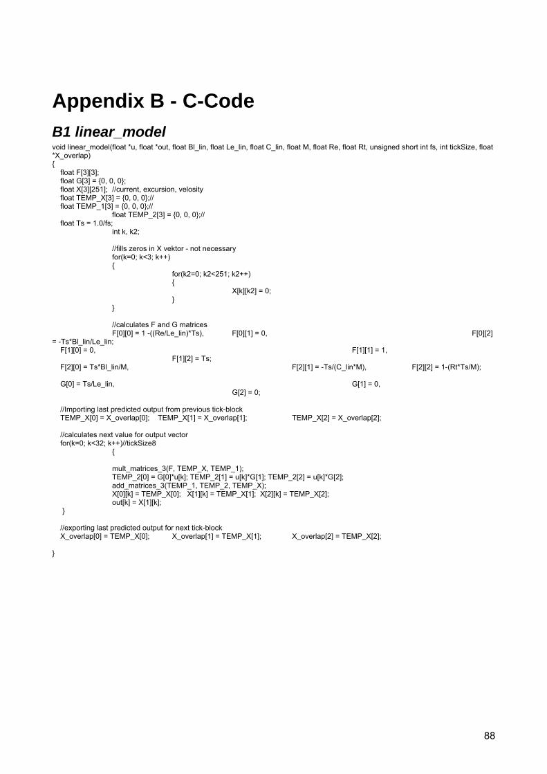
88

Appendix B - C-Code B1 linear_model void linear_model(float *u, float *out, float Bl_lin, float Le_lin, float C_lin, float M, float Re, float Rt, unsigned short int fs, int tickSize, float *X_overlap) float F[3][3]; float G[3] = 0, 0, 0; float X[3][251]; //current, excursion, velosity float TEMP_X[3] = 0, 0, 0;// float TEMP_1[3] = 0, 0, 0;// float TEMP_2[3] = 0, 0, 0;// float Ts = 1.0/fs; int k, k2; //fills zeros in X vektor - not necessary for(k=0; k<3; k++) for(k2=0; k2<251; k2++) X[k][k2] = 0; //calculates F and G matrices F[0][0] = 1 -((Re/Le_lin)*Ts), F[0][1] = 0, F[0][2] = -Ts*Bl_lin/Le_lin; F[1][0] = 0, F[1][1] = 1, F[1][2] = Ts; F[2][0] = Ts*Bl_lin/M, F[2][1] = -Ts/(C_lin*M), F[2][2] = 1-(Rt*Ts/M); G[0] = Ts/Le_lin, G[1] = 0, G[2] = 0; //Importing last predicted output from previous tick-block TEMP_X[0] = X_overlap[0]; TEMP_X[1] = X_overlap[1]; TEMP_X[2] = X_overlap[2]; //calculates next value for output vector for(k=0; k<32; k++)//tickSize8 mult_matrices_3(F, TEMP_X, TEMP_1); TEMP_2[0] = G[0]*u[k]; TEMP_2[1] = u[k]*G[1]; TEMP_2[2] = u[k]*G[2]; add_matrices_3(TEMP_1, TEMP_2, TEMP_X); X[0][k] = TEMP_X[0]; X[1][k] = TEMP_X[1]; X[2][k] = TEMP_X[2]; out[k] = X[1][k]; //exporting last predicted output for next tick-block X_overlap[0] = TEMP_X[0]; X_overlap[1] = TEMP_X[1]; X_overlap[2] = TEMP_X[2];

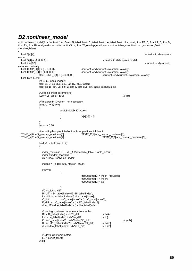
89

B2 nonlinear_model void nonlinear_model(float *u, float *out, float *Bl_tabel, float *C_tabel, float *Le_tabel, float *dLe_tabel, float R2_0, float L2_0, float M, float Re, float Rt, unsigned short int fs, int tickSize, float *X_overlap_nonlinear, short int table_size, float max_excursion,float stepsize_table) float F[4][4]; //matrice in state space model float G[4] = 0, 0, 0, 0; //matrice in state space model float X[4][32]; //current, eddycurrent, excursion, velosity float TEMP_X[4] = 0, 0, 0, 0; //current, eddycurrent, excursion, velosity float TEMP_1[4] = 0, 0, 0, 0; //current, eddycurrent, excursion, velosity float TEMP_2[4] = 0, 0, 0, 0; //current, eddycurrent, excursion, velosity float Ts = 1.0/fs; int k, k2, index, index2; float Bl, C, Le, dLe, Le0, L2, R2, dL2, factor; float dx, Bl_diff, Le_diff, C_diff, K_diff, dLe_diff, index_realvalue, K; //Loading linear parameters Le0 = Le_tabel[1600]; // [H] //fills zeros in X vektor - not necessary for(k=0; k<4; k++) for(k2=0; k2<32; k2++) X[k][k2] = 0; factor = 0.88; //Importing last predicted output from previous tick-block TEMP_X[0] = X_overlap_nonlinear[0]; TEMP_X[1] = X_overlap_nonlinear[1]; TEMP_X[2] = X_overlap_nonlinear[2]; TEMP_X[3] = X_overlap_nonlinear[3]; for(k=0; k<tickSize; k++) index_realvalue = TEMP_X[2]/stepsize_table + table_size/2; index = index_realvalue; dx = index_realvalue - index; index2 = ((index-1600)*factor +1600); if(k==3) debugbuffer[0] = index_realvalue; debugbuffer[1] = index; debugbuffer[2] = dx; //Calculating diff Bl_diff = Bl_tabel[index+1] - Bl_tabel[index]; Le_diff = Le_tabel[index+1] - Le_tabel[index]; C_diff = C_tabel[index2+1] - C_tabel[index2]; K_diff = 1/C_tabel[index2+1] - 1/C_tabel[index2]; dLe_diff = dLe_tabel[index+1] - dLe_tabel[index]; //Loading nonlinear parameters from tables Bl = Bl_tabel[index] + dx*Bl_diff; // [N/A] Le = Le_tabel[index] + dx*Le_diff; // [H] C = C_tabel[index2] + (dx*factor)*C_diff; // [m/N] K = 1.0/C_tabel[index2] + (dx*factor)*K_diff; // [N/m] dLe = dLe_tabel[index] + dx*dLe_diff; // [H/m] //Eddycurrent parameters L2 = Le*L2_0/Le0; // [H]

90

R2 = Le*R2_0/Le0; // [ohm] dL2 = dLe*L2_0/Le0; // [H/m] //calculates F matrices F[0][0] = 1-(Re+R2)/Le*Ts; F[0][1] = R2/Le*Ts; F[0][2] = 0; F[0][3] = -Ts/Le*(TEMP_X[0]*dLe+Bl);//Ts/Le*; F[1][0] = R2*Ts/L2; F[1][1] = 1-(R2*Ts/L2); F[1][2] = 0; F[1][3] = -Ts/L2*TEMP_X[1]*dL2;//1-(Rt*Ts/M); F[2][0] = 0; F[2][1] = 0; F[2][2] = 1; F[2][3] = Ts; F[3][0] = (Ts*Bl/M); F[3][1] = 0; F[3][2] = -Ts/(C*M);F[3][3] = 1-Rt*Ts/M; //calculates G matrice G[0] = Ts/Le, G[1] = 0, G[2] = 0; G[3] = 0; //multiplies G and F matrice(TEMP_1 = TEMP_X x F) mult_matrices_4(F, TEMP_X, TEMP_1); TEMP_2[0] = G[0]*u[k]; TEMP_2[1] = u[k]*G[1]; TEMP_2[2] = u[k]*G[2]; TEMP_2[3] = u[k]*G[3]; //calculates X(n+1) add_matrices_4(TEMP_1, TEMP_2, TEMP_X); //filling data to state space vector X[0][k] = TEMP_X[0]; X[1][k] = TEMP_X[1]; X[2][k] = TEMP_X[2]; X[3][k] = TEMP_X[3]; //setting output out[k] = X[2][k]; //exporting last predicted output for next tick-block X_overlap_nonlinear[0] = TEMP_X[0]; X_overlap_nonlinear[1] = TEMP_X[1]; X_overlap_nonlinear[2] = TEMP_X[2]; X_overlap_nonlinear[3] = TEMP_X[3];

91

A3. nonlinear_model_comp void nonlinear_model_comp(float *w, float *out, float *Bl_tabel, float *C_tabel, float *Le_tabel, float *dLe_tabel, float R2_0, float L2_0, float M, float Re, float Rt, unsigned short int fs, int tickSize, float *X_overlap_nonlinear, short int table_size, float max_excursion,float stepsize_table) float F[4][4]; //matrice in state space model float G[4] = 0, 0, 0, 0; //matrice in state space model float X[4][32]; //current, eddycurrent, excursion, velosity float TEMP_X[4] = 0, 0, 0, 0; //current, eddycurrent, excursion, velosity float TEMP_1[4] = 0, 0, 0, 0; //current, eddycurrent, excursion, velosity float TEMP_2[4] = 0, 0, 0, 0; //current, eddycurrent, excursion, velosity float Ts = 1.0/fs; int k, k2, index, index2; float Bl, Le, C, K; float dBl, dK, dLe, ddLe, L2, R2, dL2; float Bl0,C0,K0,Le0,P0,P1,P2,P3,P4,u,v; float dx, Bl_diff, Le_diff, C_diff, K_diff, dLe_diff, index_realvalue, factor; //Loading linear parameters Bl0 = Bl_tabel[1600]; // [N/A] Le0 = Le_tabel[1600]; // [H] C0 = C_tabel[1600]; // [m/N] K0 = 1.0/C0; // [N/m] //fills zeros in X vektor - not necessary but... for(k=0; k<4; k++) for(k2=0; k2<32; k2++) X[k][k2] = 0; //Importing last predicted output from previous tick-block TEMP_X[0] = X_overlap_nonlinear[0]; TEMP_X[1] = X_overlap_nonlinear[1]; TEMP_X[2] = X_overlap_nonlinear[2]; TEMP_X[3] = X_overlap_nonlinear[3]; factor = 0.88; for(k=0; k<tickSize; k++) //calculating index for tables, from excursion[m] //index = TEMP_X[2]/stepsize_table + table_size/2 + 0.5; index_realvalue = TEMP_X[2]/stepsize_table + table_size/2; index = index_realvalue; dx = index_realvalue - index; index2 = index;//((index-1600)*factor +1600); //Calculating diff Bl_diff = Bl_tabel[index+1] - Bl_tabel[index]; Le_diff = Le_tabel[index+1] - Le_tabel[index]; C_diff = C_tabel[index2+1] - C_tabel[index2]; K_diff = 1/C_tabel[index2+1] - 1/C_tabel[index2]; dLe_diff = dLe_tabel[index+1] - dLe_tabel[index]; //Loading nonlinear parameters from tables Bl = Bl_tabel[index] + dx*Bl_diff; // [N/A] Le = Le_tabel[index] + dx*Le_diff; // [H] C = C_tabel[index2] + dx*C_diff*factor; // [m/N] K = 1.0/C_tabel[index2] + dx*K_diff*factor; // [N/m] dLe = dLe_tabel[index] + dx*dLe_diff; // [H/m] //Calculation derivatives, (dLe is loaded from table) dBl = Bl_diff/stepsize_table; // [N/Am] dK = K_diff/stepsize_table; // [N/m2] ddLe = dLe_diff/stepsize_table; // [H/m2] //Eddycurrent parameters

92

L2 = Le*L2_0/Le0; // [H] R2 = Le*R2_0/Le0; // [ohm] dL2 = dLe*L2_0/Le0; // [H/m] //Compensator u = Le/(Bl+dLe*TEMP_X[0])*(TEMP_X[3]*(TEMP_X[2]*dK + (K-K0) - dBl*TEMP_X[0] - ddLe*(TEMP_X[0]*TEMP_X[0])/2 - (Bl0*Bl0)/Le0) + Re*TEMP_X[2]*(K-K0)/Le0 - Re*TEMP_X[0]*(2*Bl+dLe*TEMP_X[0])/(2*Le0) + Bl0*w[k]/Le0) + Re*TEMP_X[0] + Bl*TEMP_X[3] + dLe*TEMP_X[0]*TEMP_X[3] + R2*(TEMP_X[0]-TEMP_X[1]); //calculates F matrise F[0][0] = 1-(Re+R2)/Le*Ts; F[0][1] = R2/Le*Ts; F[0][2] = 0; F[0][3] = -Ts/Le*(TEMP_X[0]*dLe+Bl);//Ts/Le*; F[1][0] = R2*Ts/L2; F[1][1] = 1-(R2*Ts/L2); F[1][2] = 0; F[1][3] = -Ts/L2*TEMP_X[1]*dL2;//1-(Rt*Ts/M); F[2][0] = 0; F[2][1] = 0; F[2][2] = 1; F[2][3] = Ts; F[3][0] = (Ts*Bl/M); F[3][1] = 0; F[3][2] = -Ts/(C*M);F[3][3] = 1-Rt*Ts/M; //calculates G matrise G[0] = Ts/Le, G[1] = 0, G[2] = 0; G[3] = 0; //multiplies G and F matrice(TEMP_1 = TEMP_X x F) mult_matrices_4(F, TEMP_X, TEMP_1); TEMP_2[0] = u*G[0]; TEMP_2[1] = u*G[1]; TEMP_2[2] = u*G[2]; TEMP_2[3] = u*G[3]; //calculates X(n+1) add_matrices_4(TEMP_1, TEMP_2, TEMP_X); //filling data to state space vector X[0][k] = TEMP_X[0]; X[1][k] = TEMP_X[1]; X[2][k] = TEMP_X[2]; X[3][k] = TEMP_X[3]; //setting output out[k] = u;//X[2][k]; //exporting last predicted output for next tick-block X_overlap_nonlinear[0] = TEMP_X[0]; X_overlap_nonlinear[1] = TEMP_X[1]; X_overlap_nonlinear[2] = TEMP_X[2]; X_overlap_nonlinear[3] = TEMP_X[3];

B4 get_linear_parameters //loudspeaker B(8480277) *Re = 5.02882; *L2 = 0.000565304; *R2 = 2.67697; *Rt = 2.25391; *M = 0.0195471; *Le_lin = 0.000389793; *C_lin = 0.000538315; *Bl_lin = 7.18583;

93

B5 get_nonlinear_parameters void get_nonlinear_parameters(float *Bl, float *C, float *Le, float *dLe, short int table_size, float max_excursion,float stepsize_table) short int i; float x=0; //polynomes for nonlinear parameters //31211 //float Le_p[9] = 0.58157, -0.031046, -0.0066093, 0.0011830, 0.00042152, -0.00015811, -6.4289e-5, 1.1929e-5, 4.5528e-6; //float Bl_p[9] = 7.03, -0.023848, -0.055244, 0.0099365, -0.0042554, -0.00014267, 9.478e-5, -7.2017e-6, 2.3069e-7; //float C_p[9] = 0.241, 0.0045478, -0.0050385, 0.00022905, 0.00012458, -0.10724e-4, -2.6118e-6, 2.8368e-7, 0.6371e-8; //8084277 //float Le_p[9] = 4.42852e-004, -3.99246e-003, -0.730067, 11.3856, 2426.82, -8064.92, -3.80829e+007, 1.0525e+008, 3.24411e+011; //float Bl_p[9] = 7.19845, -22.7689, -10185.5, 3.70864e+006, -1.65104e+009, -5.0827e+010, 2.04298e+013, 1.40152e+014, -7.96303e+016; //float C_p[9] = 1.12474e-003, 1.91161e-002, -33.3252, -1199.15, 636426, 2.74833e+007, -7.21205e+009, -2.23333e+011, 3.37872e+013; float Le_p[9] = 5.82481e-004, -7.58251e-003, 0.277347, 38.1499, -695.65, -1.7902e+006, -7.5998e+007, 4.13538e+010, 3.36663e+012; float Bl_p[9] = 7.18999, -5.79654, -13760.8, 1.21422e+006, -1.15292e+009, -5.35162e+009, 6.48184e+012, -2.18535e+014, 8.14653e+016; float C_p[9] = 1.20736e-003, 5.33297e-002, -43.9281, -4956.1, 1.02868e+006, 2.04476e+008, -1.12013e+010, -3.53739e+012, -6.31026e+013; //creating tabells for nonlinear parameters for(i=0; i<table_size; i++) x = (i-table_size/2)*stepsize_table; //(i-1600)/160000.0; Bl[i] = Bl_p[0] + Bl_p[1]*x + Bl_p[2]*pow(x,2) + Bl_p[3]*pow(x,3) + Bl_p[4]*pow(x,4) + Bl_p[5]*pow(x,5) + Bl_p[6]*pow(x,6) + Bl_p[7]*pow(x,7) +Bl_p[8]*pow(x,8); C[i] = C_p[0] + C_p[1]*x + C_p[2]*pow(x,2) + C_p[3]*pow(x,3) + C_p[4]*pow(x,4) + C_p[5]*pow(x,5) + C_p[6]*pow(x,6) + C_p[7]*pow(x,7) +C_p[8]*pow(x,8); Le[i] = Le_p[0] + Le_p[1]*x + Le_p[2]*pow(x,2) + Le_p[3]*pow(x,3) + Le_p[4]*pow(x,4) + Le_p[5]*pow(x,5) + Le_p[6]*pow(x,6) + Le_p[7]*pow(x,7) +Le_p[8]*pow(x,8); dLe[i]= Le_p[1] + 2*Le_p[2]*x + 3*Le_p[3]*pow(x,2) + 4*Le_p[4]*pow(x,3) + 5*Le_p[5]*pow(x,4) + 6*Le_p[6]*pow(x,5) + 7*Le_p[7]*pow(x,6) + 8*Le_p[8]*pow(x,7);

B6 Gain void Gain(float *Gain, float *table, int table_Size) int i; float sum = 0; for(i=0;i<table_Size;i++) sum = sum + table[i]; *Gain = sum/table_Size;

94

B7 Peak void Peak(float *Peak, float *table, int table_Size, unsigned short int tickSize) int i; float P=0; for(i=0; i<table_Size; i++) //summing one tick if(table[i]>P) P = table[i]; *Peak = P/tickSize;

B8 Rms void Rms(float *Rms, float *table, int table_Size, unsigned short int fs) int i; float sum=0; for(i=0; i<table_Size; i++) sum = sum + table[i]; *Rms = sqrt(sum/(fs));

B8 add_matrices_3 void add_matrices_3(float a[3], float b[3], float result[3]) int i, j; for(i=0; i<3; i++) result[i] = 0; for(i=0; i<3; i++) result[i] = a[i] + b[i];

B9 mult_matrices_3 void mult_matrices_3(float a[3][3], float b[3], float result[3]) int i, k; for(i=0; i<3; i++) result[i] = 0; for(i=0; i<3; i++) for(k=0; k<3; k++)

95

result[i] = result[i] + a[i][k] * b[k];

B10 add_matrices_4 void add_matrices_4(float a[4], float b[4], float result[4]) int i, j; for(i=0; i<4; i++) result[i] = 0; for(i=0; i<4; i++) result[i] = a[i] + b[i];

B11 mult_matrices_4 void mult_matrices_4(float a[4][4], float b[4], float result[4]) int i, k; for(i=0; i<4; i++) result[i] = 0; for(i=0; i<4; i++) for(k=0; k<4; k++) result[i] = result[i] + a[i][k] * b[k];

96

B12 main //constant parameters float X_overlap[3] = 0, 0, 0, X_overlap_nonlinear[4] = 0, 0, 0, 0; unsigned short int fs = 48000, f = 50; unsigned short int table_size = 3200; float max_excursion = 0.02, stepsize_table; //Storage last value of tick. float *X_overlappk = &X_overlap[0]; float *X_overlap_nonlinear_pk = &X_overlap_nonlinear[0]; float testin[1100], testout[110], model[110], pi = 3.1415927; float *testinpk = &testin[0], *testoutpk = &testout[0], *modelpk = &model[0]; float Bl[3200], C[3200], Le[3200], dLe[3200];//, dC[3200], dBl[3200], ddLe[3200]; int i,init = 0, index=0, Rms_table_Size, counter1=0; float x, P_Amp_Gain = 1, u_ticksum=0, u_Peak_tick=0, u_Peak=0, u_Rms=0, u_tab[1500]; float x, U_measured_ticksum=0, U_measured_Peak_tick=0, U_measured_Peak=0, U_measured_Rms=0, U_measured_tab[1500]; float Rms_vindowtime = 1, Gain_tab[1500], C_old[3200], C_change; float W[32], U[32], Model[32], Gain_feedback=37, Limiter=1, peak=0; SEG_MOD_FAST_CODE static void AMF_compensator_Render(AMF_compensator * restrict instance,float * restrict * buffers,int tickSize) int i; float *w = buffers[0]; // Don't use restrict because we say they can alias (see .h file) float *U_measured = buffers[1]; float *in3 = buffers[2]; float *in4 = buffers[3]; float *u = buffers[4]; float *w2 = buffers[5]; float *Model = buffers[6]; float *out4 = buffers[7]; float compliance_scaler = instance->compensatoramp; //float compliance = instance->compliance; //initialisering if(init==0) // stepsize_table = (2*max_excursion)/table_size; //Loading linear parameters, 31211 is default get_linear_parameters(&Re,&L2,&R2,&M,&Rt,&Bl_lin,&Le_lin,&C_lin); //Loading Nonlinear parameters tabels get_nonlinear_parameters(Bl, C, Le, dLe, table_size,max_excursion,stepsize_table); //changes in compliance C_change = 0.001; for(i=0; i<table_size; i++) C_old[i] = C[i]; //calculating Rms, Peak, P.Amp-Gain.... u_ticksum=0, U_measured_ticksum=0; //Setting Gain / (input signal) P_Amp_Gain = 8.944; //controlling index init++; index++;

97

if(index>Rms_table_Size) init = 1; index = 0; //Simulating the Power Amplifier by scaling the input signal for(i=0; i<tickSize; i++) w[i] = P_Amp_Gain*w[i]; //gain controll - input //Scaling the complianse //uptuning if(C[1600] < (C_old[1600]*compliance_scaler)-(C_change*0.001) ) for(i=0; i<table_size; i++) C[i] = C[i] + (C[i] * C_change); counter1++; //downtuning if(C[1600] > (C_old[1600]*compliance_scaler)+(C_change*0.001) ) for(i=0; i<table_size; i++) C[i] = C[i] - (C[i] * C_change); counter1++; //Comparator/Nonlinear linearization //linear_model(W, U, Bl_lin, Le_lin, C_lin, M, Re, Rt, fs, tickSize, X_overlap); nonlinear_model_comp(w, testoutpk, Bl, C, Le, dLe, R2, L2, M, Re, Rt, fs, tickSize,X_overlap_nonlinear,table_size,max_excursion,stepsize_table); //nonlinear_model(w, modelpk, Bl, C, Le, dLe, R2, L2, M, Re, Rt, fs, tickSize,X_overlap_nonlinear,table_size,max_excursion,stepsize_table); //Reducing signal before the real Power Amplifier. peak = 0; for (i=0; i<tickSize; i++) //u[i] = testoutpk[i]; u[i] = testoutpk[i]*1/P_Amp_Gain; //u[i]= 1000*modelpk[i];//Model[i] w2=w; SEG_MOD_SLOW_CONST const AMF_ModuleClass AMFClasscompensator = /* Flags */ 0, /* Render function */ (AMF_RenderFunction)AMF_compensator_Render, // render function /* Default bypass */ (void *)0, /* Input descriptor - 1 input, and it is mono. */ 1, 0, /* Output descriptor - 1 output, and it is mono. */ 1, 0,

Compensation of Loudspeaker Nonlinearities.pdf

Documents

Transcript of Compensation of Loudspeaker Nonlinearities.pdf