i

ii

Compensating the Effect of Control Valve Stiction

by

Ahaduzzaman

(1015022040 P)

MASTER OF SCIENCE IN ENGINEERING

(CHEMICAL)

Department of Chemical Engineering

BANGLADESH UNIVERSITY OF ENGINEERING AND TECHNOLOGY

June, 2018

iii

CERTIFICATION OF THESIS WORK

The thesis titled ''Compensating the Effect of Control Valve Stiction'' submitted by

Ahaduzzaman Roll No. 1015022040P Session October, 2015 has been accepted as

satisfactory in partial fulfillment of the requirement for the degree of Master of Science

in Engineering (Chemical) on June 3, 2018.

BOARD OF EXAMINERS

Dr. Md. Ali Ahammad Shoukat Choudhury Professor Department of Chemical Engineering BUET, Dhaka-1000

Chairman

Dr. Ijaz Hossain Professor and Head Department of Chemical Engineering BUET, Dhaka-1000

Member (Ex-officio)

Sirajul Haque Khan Associate Professor Department of Chemical Engineering BUET, Dhaka-1000

Member

Sk. Shafi Ahmed B.Sc. Engg. & M.Sc. Engg. (BUET) Ex-COO, KAFCO Flat 4B; SEL Sobhan Place, 2B Golden Street Shamoli, Dhaka, Bangladesh

Member (External)

iv

DECLARATION

The thesis on “Compensating the effect of Control Valve Stiction” completed by

Ahaduzzaman has been submitted in partial fulfillment of the degree of Master of

Science in Chemical Engineering. This thesis is my original work and wherever

contributions of others are involved, every effort is made to indicate this clearly, with due

reference to the literature, and acknowledgement of collaboration is made explicitly.

Ahaduzzaman

St ID: 1015022040 P

Department of Chemical Engineering

Bangladesh University of Engineering and Technology

In my capacity as supervisor of the candidate’s thesis, I certify that the above statements

are true to the best of my knowledge.

Thesis supervisor

Dr. M. A. A. Shoukat Choudhury

Professor

Department of Chemical Engineering

Bangladesh University of Engineering and Technology

Dhaka -1000

v

ACKNOWLEDGEMENTS

At first I would like to express my heartiest gratitude to the almighty Allah for enabling

me to complete my thesis work successfully.

There are several people that I would like to acknowledge, without whom I would not

have succeeded in preparing this work. I would like to express my most sincere gratitude

to my supervisor; Professor Dr. M. A. A. Shoukat Choudhury for his inspiration,

instruction, support and guidance to make progress which has been a great motivation

during my work. I am deeply indebted to him for his sincere effort to teach me the art of

doing research works. His patience, enthusiasm, immense knowledge and

encouragements have carried me always.

I would also like to gratefully acknowledge Mr. B.M.Sirajeel Arifin, Ex- Lecturer,

Department of Chemical Engineering, BUET, Malik Mohammad Tahiyat, Ex-Teaching

assistant, Department of Chemical Engineering, BUET, Md. Habibur Rahman, Executive

Engineer, ERL and Ashfaq Iftekhar Udoy for sharing their knowledge and supporting me

during the thesis work.

Most of all, I wish to thank my parents and family members. Their concern,

encouragement, and advice will always be remembered.

vi

ABSTRACT

Valve stiction is the hidden culprit of the process control loop. The presence of stiction in

a control valve limits the control loop performance. It is the most commonly found

problem in pneumatic control valves. It decreases the control loop efficiency and causes

oscillations in process variables. Repair and maintenance is the only definitive solution to

fix a sticky valve. However, this fact implies to stop the operation of the control loop,

which is only possible during plant shutdown. Compensation of its effect is beneficial

before the sticky valve can be sent for maintenance. In this study, a new stiction

compensation method has been developed by adding an extra pulse for a certain period of

time to the detuned controller action. A method for estimating the parameters required for

the proposed compensator has also been developed. The performance of the proposed

stiction compensation scheme is evaluated using MATLAB Simulink software. The

developed compensator has the desired capability of reducing the process variability with

a minimum number of valve reversals. It has the capability of good set-point tracking and

disturbance rejection. The performance of the proposed compensator has been compared

with other compensators available in the literature. The proposed compensator

outperforms all of other compensators. The proposed compensator has been implemented

to a level control loop in a pilot plant experimental set-up. It has been found to be

successful in removing valve stiction induced oscillations from process variables.

Moreover, the proposed compensation scheme is simple. It requires minimum process

knowledge. It would not be difficult to implement it in real process plants.

vii

TABLE OF CONTENTS

Contents Page No.

Acknowledgement ..............................................................................................................v

Abstract ............................................................................................................................. vi

Table of Contents ............................................................................................................. vii

List of Figures .................................................................................................................... xi

List of Tables ................................................................................................................... xiv

Nomenclature .................................................................................................................... xv

Abbreviations ................................................................................................................... xvii

CHAPTER 1 INTRODUCTION 1-10

1.1 Background ..................................................................................................................1

1.2 What is Stiction? ..........................................................................................................2

1.2.1 Definition of Terms Relating to Valve Stiction ..................................................2

1.2.2 Mechanism of Stiction .........................................................................................4

1.2.3 Where does Stiction Occurs in Control Valve? ...................................................6

1.3 Stiction Compensation .................................................................................................7

1.4 Objectives of the Study ..............................................................................................9

1.5 Objectives of the Study ..............................................................................................9

1.6 Chapter Summary .....................................................................................................10

CHAPTER 2 LITERATURE REVIEW 11-29

2.1 The Knocker .............................................................................................................11

2.2 Two Move Method ...................................................................................................13

2.3 Constant Reinforcement Method ...............................................................................14

2.4 Modified Two Moves Method ..................................................................................15

2.5 Improved Two Move Method .................................................................................16

2.6 Three Move Method ..................................................................................................17

viii

Contents Page No.

2.7 Improved Knocker and CR Method ..........................................................................18

2.8 Improved Knocker Method .......................................................................................20

2.9 Model Free Stiction Compensation Method ..............................................................21

2.10 Method for Compensating Stiction Nonlinearity ...................................................23

2.11 Six Moves Method ..................................................................................................24

2.12 Four Moves Method ................................................................................................25

2.13 Variable Amplitude Pulses Method .........................................................................26

2.14 Summary of the Available Stiction Compensation Methods .................................28

2.15 Chapter Summary ...................................................................................................29

CHAPTER 3 DEVELOPING A COMPENSATING TECHNIQUES FOR

CONTROL VALVE STICTION 30-43

3.1 Compensation Scheme ..............................................................................................30

3.2 Dealing with Stochastic or Noisy control Signals .....................................................34

3.3 Choice of Compensator Parameters .........................................................................34

3.3.1 Parameters for Pulse Generator ........................................................................35

3.3.2 Specified Time Limit, TG ..................................................................................35

3.3.3 Permissible error, ϵ ..........................................................................................36

3.3.4 Detuning parameter, α ......................................................................................36

3.3.4.1 Estimation of Detune Parameter, α ...........................................................38

3.4 Initialization of Compensator ...................................................................................42

3.5 Chapter Summary .....................................................................................................43

ix

Contents Page No.

CHAPTER 4 PERFORMANCE EVALUATION OF THE PROPOSED

COMPENSATOR 44-52

4.1 Evaluation of Performance of Compensator for FOPTD Process .............................44

4.2 Evaluation of the Performance of the Compensator for different FOPTD process ..46

4.3 Evaluation of the Compensator Performance for Different Perturbations ................48

4.3.1 Set Point Tracking .............................................................................................48

4.3.2 Disturbance Rejection .......................................................................................49

4.3.3 Sensitivity to Noise ...........................................................................................50

4.3.4 Sensitivity to Extent of Stiction .........................................................................51

4.4 Chapter Summary .....................................................................................................52

CHAPTER 5 COMPARISON OF THE PERFORMANCE OF DIFFERENT

COMPENSATION METHODS 53-62

5.1 Stiction Compensators ...............................................................................................53

5.2 Comparison of Trend Analysis ..................................................................................54

5.3 Comparison of Performance ......................................................................................57

5.4 Comparison of the Proposed Method and Capaci et al. Method ...............................59

5.4.1 Disturbance Rejection Capability ......................................................................60

5.4.2 Uncertainty in Stiction Amount .........................................................................61

5.4.3 Non-Homogeneous Stiction ...............................................................................62

5.5 Chapter Summary ......................................................................................................62

x

Contents Page No.

CHAPTER 6 EXPERIMENTAL EVALUATION OF THE PROPOSED

COMPENSATION METHOD 63-72

6.1 Description of the Plant .............................................................................................63

6.2 Operating Procedure ..................................................................................................66

6.3 Model Identification ..................................................................................................66

6.4 PI(D) Controller Design ............................................................................................68

6.5 Experimental Evaluation ............................................................................................69

6.6 Chapter Summary ......................................................................................................72

CHAPTER 7 CONCLUSION AND RECOMMENDATION FOR FUTURE

WORK 73-74

7.1 Conclusion ...................................................................................................................73

7.2 Recommendation for Future Work ..............................................................................74

REFERENCES ............................................................................................................ 75-76

APPENDICES 77-82

APPENDIX A ....................................................................................................................77

APPENDIX B ...................................................................................................................78

APPENDIX C ...................................................................................................................79

APPENDIX D ...................................................................................................................80

APPENDIX E ...................................................................................................................81

APPENDIX F ....................................................................................................................82

xi

LIST OF FIGURES

Figure No. Title of the Figure Page No.

Figure 1.1 Global Multi-Industry Performance Demography .......................................2

Figure 1.2 Typical input–output behavior of hysteresis, dead band and dead zone ......4

Figure 1.3 Typical input–output behavior of a sticky valve..........................................5

Figure 1.4 A cross sectional diagram of a spring-diaphragm pneumatic control valve 6

Figure 2.1 Block diagram illustrating the knocker used in a feedback loop ...............11

Figure 2.2 Pulse sequence characterization of Knocker method.................................12

Figure 2.3 Control loop with a two move method compensator .................................13

Figure 2.4 Block diagram for CR approach ................................................................15

Figure. 2.5 Wave-shape of Karthiga and Kalaivani, (2012) compensation method ....17

Figure 2.6 Decision flow diagram of the improved knocker and CR method ............18

Figure 2.7 Block diagram illustrating the improved knocker and CR compensation

method........................................................................................................19

Figure 2.8 Waveform of the improved knocker method .............................................20

Figure 2.9 Stiction compensation strategies of Arifin et al., (2014) method ..............21

Figure 2.10 Signal flow path for computation of the error signal .................................21

Figure 2.11 Signal flow path for computation of the control signal uc .........................22

Figure 2.12 Closed loop control system with stiction compensator using sinusoidal

signal ..........................................................................................................23

Figure 2.13 Flow chart of actuator stiction compensation via variables amplitude

pulse ...........................................................................................................26

Figure 3.1 Block diagram illustrating the proposed model .........................................31

Figure 3.2 Signal from controller, pulse generator and compensator .........................32

xii

Figure No. Title of the Figure Page No.

Figure 3.3 Zoomed version of Figure 3.2 ....................................................................32

Figure 3.4 Simulink block diagram of the proposed compensator..............................33

Figure 3.5 Flowchart for the proposed compensator model ........................................33

Figure 3.6 Pulse sequence characterization of the proposed method. .........................35

Figure 3.7 Process output response curve of a single first order process for three

different case of α ......................................................................................37

Figure 3.8 Minimum IAE of different process for selected detune parameter, α .......39

Figure 3.9 Minimum SSE for different number of Emperical Models .....................41

Figure 3.10 Process output response for the proposed model without initialization ....42

Figure 3.11 Process output response for the proposed model with initialization ..........42

Figure 4.1 Simulink block diagram for evaluating the performance of proposed

compensator ...............................................................................................45

Figure 4.2 Simulation results for the proposed compensator of a single FOPTD

process........................................................................................................45

Figure 4.3 Sample results for different FOPTD model ......................................... 46-47

Figure 4.4 Stiction compensation for set-point tracking .............................................48

Figure 4.5 Results for proposed compensator when a step disturbance is added

at 7000 s .....................................................................................................49

Figure 4.6 The output response of a process when high variance level of noise is

added ..........................................................................................................50

Figure 5.1: Response curve of output process variable, PV and set point, SP for

different compensator model ............................................................... 54-55

Figure 5.2: Response curve of valve position, MV and controller output, OP for

different compensator model .....................................................................56

Figure 5.3 Unit step disturbance rejection capability for Capaci et al. (2016)

method........................................................................................................60

xiii

Figure No. Title of the Figure Page No.

Figure 5.4 Unit step disturbance rejection capability for proposed compensator

method........................................................................................................60

Figure 5.5 Process response curve of unknown stiction parameter for Capaci et al.

(2016) method. ...........................................................................................61

Figure 5.6 Process response curve for proposed method for the case of unknown

stiction parameters .....................................................................................61

Figure 5.7 Simulation results of proposed model for non-homogeneous stiction

parameters ..................................................................................................62

Figure 6.1 Experimental set-up of the water level control system ..............................63

Figure 6.2 Schematic diagram of the water level control system ...............................63

Figure 6.3 Simulink block diagram of a level control feedback loop .........................65

Figure 6.4 Simulink block diagram of open loop configuration. ................................66

Figure 6.5 The open loop response curve for the pilot plant .......................................66

Figure 6.6 The process output results for non-sticky condition using final controller

settings .......................................................................................................68

Figure 6.7: Simulink block diagram for the implementation of proposed

compensator ...............................................................................................68

Figure 6.8 Experimental results of the proposed compensator ...................................70

xiv

LIST OF TABLES

Table No. Title of the Table Page No. Table 2.1 Table for various feature of available stiction compensation methods.. ....28

Table 4.1 Effect of noise on stiction compensation ...................................................50

Table-4.2 Impact of stiction parameters on stiction compensation ............................51

Table-5.1 Integral Absolute Error, IAE data for different compensator model .........58

Table-5.2 Variance of output process variable, 𝜎2 data for different compensator

…………. model..........................................................................................................58

Table-5.3 Valve Travel, VT data for different compensator model. ..........................59

Table 6.1: Process Variable variance for different conditions ....................................71

xv

NOMENCLATURE

GP Process Transfer Function

GC Controller Transfer Function

Gk Knocker Transfer Function

Gf Filter Transfer Function

ysp (t) Desired Set-Point

y(t) Process Output

uk(t) Knocker Output

hk Pulse Period

𝜏𝑑 Pulse Width

d Stiction Parameter

u(t) Summation of Knocker and Controller Output

uc Controller Output

OP Compensator Output

PV Process Variable

SP Set-Point

MV Valve Position

S Deadband plus Stickband

J Slip Jump

KP Process Gain

𝜏 Time Constant

𝜃 Time Delay

KC Controller Gain

Ts Sample Time

TP Time of One Set of Previous Pulse

TG Specific Time during which Pulse Generator Remains Activated

𝜖 Permissible Error

e Difference Between Set-point and Process Output, (SP-PV)

AP Pulse Amplitude

α Detune Parameter

N Total Number of Data Points

xvi

µ Mean Value of Process Variable

x Valve Position

𝜎2 Process Variable Variance

η Performance Index

P(s) Process Transfer Function

C(s) Controller Transfer Function

xvii

ABBREVIATIONS

EWMA Exponentially Weighted Moving Average

FOPTD First Order Plus Time Delay

IAE Integral Absolute Error

IMC Internal Model Control

PI(D) Proportional Integral

PID Proportional Integral Derivative

VT Valve Travel

SISO Single Input Single Output

SSE Summation of Square Error

1

INTRODUCTION

1.1 Background

Constrained resources, stringent environmental regulations and tough business

competition have resulted in efficient manufacturing operations in terms of energy usage,

raw material utilization, superior quality products and plant safety. Most of the modern

plants are now automated to achieve these goals. Control loops are the essential part of

these automated processes. Large-scale, highly integrated processing plants include

hundreds or thousands of such control loops.

The aim of each control loop is to maintain the process at the desired operating

conditions safely and efficiently. A poorly performing control loop can result in

disrupted process operation, degraded product quality, higher material or energy

consumption. Thus the poor performance of the control loop decreases plant profitability.

Control loop performance has been an active research area for academia and industry for

the last three decades. Control loops often suffer from poor performance due to process

non-linearities, process disturbances, poorly tuned controllers and misconfigured control

strategies. Performance of over 26,000 PID controllers from a wide range of continuous

process industries was investigated by Desborough, et al. (2001). It was found that the

performance of over two thirds of control loops was not satisfactory. Another survey by

Bialkowski (1993) also reported that only one third of industrial controllers provided

acceptable performance. These survey results are shown in Figure 1.1, where the left

panel shows the survey result of Bialkowski (1993) and the right panel shows the survey

result of Desborough et al. (2001).

1 CHAPTER

2

.

Figure 1.1: Global Multi-Industry Performance. Oscillatory variables are one of the main causes for poor performance of control

loops. The presence of oscillations in a control loop increases the variability of the

process variables, which makes it difficult to keep operating conditions close to their

bounds. The reason for oscillations in a control loop may be due to poor controller

tuning, poor process and control system design, valve non-linearities, oscillatory

disturbances and other causes (Choudhury et al., 2005). Among various valve

nonlinearities, stiction is the most commonly encountered one. Hence, it is practically

very important to find the loops where control valves are sticky and thereby compensate

stiction to reduce its negative effect.

1.2 What is Stiction?

The word “Stiction” comes by combining two words-Static and Friction. Stiction is the

static friction that keeps an object from moving. When the external force to the object

overcomes the static friction, it starts moving. Often stiction is confused with some

similar problems such as backlash, hysteresis, deadband and deadzone. Therefore, these

terms are defined below for a better understanding of the term ‘stiction’.

1.2.1 Definition of Terms Relating to Valve Stiction

According to the Instrument Society of America (ISA) (ISA Committee SP51, 1979) the

definitions of the terms backlash, hysteresis, deadband and deadzone are as follows:

Bialkowski (1993) Desborough et al. (2001)

3

Backlash: “In process instrumentation, it is a relative movement between interacting

mechanical parts, resulting from looseness, when the motion is reversed”.

Hysteresis: Hysteresis is that property of the element evidenced by the dependence of the

value of the output, for a given excursion of the input, upon the history of prior

excursions and the direction of the current traverse. It is usually determined by

subtracting the value of deadband from the maximum measured separation between

upscale going and downscale going indications of the measured variable (during a full

range traverse, unless otherwise specified) after transients have decayed”. Figure 1.2(a)

and 1.2(c) illustrate the concept. Some reversal of output may be expected for any small

reversal of input. This distinguishes hysteresis from deadband.

Deadband: “In process instrumentation, it is the range through which an input signal

may be varied, upon reversal of direction, without initiating an observable change in

output signal”. There are separate and distinct input-output relationships for increasing

and decreasing signals (Figure1.2 (b)). Deadband produces phase lag between input and

output”. Deadband is usually expressed in percent of span. Deadband and hysteresis may

be present together. In that case, the characteristics in Figure 1.2(c) will be observed

Deadzone: “It is a predetermined range of input through which the output remains

unchanged, irrespective of the direction of change of the input signal”. “There is but one

input-output relationship as shown in Figure 1.2(d). Deadzone produces no phase lag

between input and output.

The above definitions show that the term “backlash” specifically applies to the slack or

looseness of the mechanical part when the motion changes its direction. Therefore, in

control valves it may only add deadband effects if there is some slack in rack-and-pinion

type actuators. Deadband is quantified in terms of input signal span (i.e., on the x-axis)

while hysteresis refers to a separation in the measured output response (i.e., on the y-

axis).

4

Figure 1.2 Typical input–output behavior of hysteresis, dead band and dead zone (ISA Committee SP51, 1979).

1.2.2 Mechanism and Definition of Stiction

As discussed above, the Instrument Society of America (ISA) (1979) provided the phase

plots for the hysteresis, deadband and deadzone as shown in Figure 1.2. There was no

such phase plot for stiction. Choudhury et al. (2005) provided the phase plot of the input–

output behavior of a valve suffering from stiction as shown in Figure 1.3. It consists of

four components: deadband, stickband, slip jump and the moving phase. When the valve

comes to restore changes the direction at point A in Figure 1.3, the valve becomes stuck.

The valve output remains same though the valve input keeps changing. The input of the

valve is generally the controller output. After the controller output (valve input)

overcomes the deadband (AB) and the stickband (BC) of the valve, the valve jumps to a

new position (point D) and continues to move. Due to very low or zero velocity, the valve

may stick again in between points D and E while travelling in the same direction. In such

5

a case, the magnitude of deadband is zero and only stick band is present. This can be

overcome if the controller output signal is larger than the stickband only (Choudhury, et

al., 2005). The deadband and stickband represent the behavior of the valve when it is not

moving, though the input to the valve keeps changing. Slip jump represents the abrupt

release of potential energy stored in the actuator chambers due to high static friction in

the form of kinetic energy as the valve starts to move. The magnitude of the slip jump is

very crucial in determining the limit cyclic behavior introduced by stiction. Once the

valve slips, it continues to move until it sticks again (point E in Figure 1.3). In this

moving-phase, dynamic friction is present which may be much lower than the static

friction. When the controller signal changes its direction, the valve behavior would be

same as before in reverse direction to the path EFGH in Figure 1.3. Thus stiction is

defined as a property of an element such that its smooth movement in response to a

varying input is preceded by a sudden abrupt jump called the slip-jump. Slip-jump is

expressed as a percentage of the output span. Its origin in a mechanical system is static

friction which exceeds the dynamic friction during smooth movement.

Figure 1.3: Typical input–output behavior of a sticky valve (Choudhury et al., 2005).

6

In industry, stiction is measured as a certain percentage of the valve travel or the span of

the control signal. For example, 2% stiction means that when valve gets stuck it will start

moving only after the cumulative change of its control signal is greater than or equal to

2%. If the range of the control signal is 4 to 20 mA then 2% stiction means a cumulative

change of the control signal less than 0.32 mA in magnitude will not be able to move the

valve.

1.2.3 Where does Stiction Occur in Control Valve?

The cross- sectional diagram of a control valve is shown in Figure 1.4.

Figure 1.4: A cross sectional diagram of a spring-diaphragm pneumatic control valve (Choudhury et al., 2008).

As shown in Figure 1.4, the valve stem moves up and down through the packing box to

restrict the flow of process fluid through the pipe. The packing stops process fluid from

Stiction

Fluid in Fluid out

Valve Stem

Packing

Stiction

7

leaking out of the valve but the valve stem nevertheless has to move freely relative to the

packing. There is a trade-off because too tight packing reduces emissions and leaks from

the valve but at the same time increases the friction. Loose packing reduces the friction

but there is a potential for process fluids to leak. Stiction happens when the smooth

movement of the valve stem is hindered by excessive static friction at the gland packing

section (Arumugam et al., 2014). So, stiction appears in the packing boxes around the

valve stem (Choudhury et al., 2005). There is a possibility of leaking the fluid in hard

packing. To avoid leakage, the packing boxes are often tightened after some period of

operation. Stiction can appear due to tightened hard packing in the control valve.

In ball valves, ball segment valves, and throttle valves there is often also a significant

friction between the ball/throttle and the seat. The friction in the pilot valve may also

increase and cause problems if the air is polluted. Hysteresis may appear at several places

in the mechanical configuration due to wear and vibrations. The stiction varies both in

time and between different operating points. Temperature variations cause friction

variations. A high temperature means that the material expands, and therefore the friction

force increases. Some media give fouling that increases the friction. Particles in the

media may cause damage on the valve. The wear is often non-uniform. Therefore,

friction is different at different valve positions. Experimental investigations showed that

the force required to overcome stiction is dependent on the rate at which the force is

applied.

Stiction is a major problem in control valve. It reduces the performance of the control

loop. Compensation of such problem is the main objective of this research work.

1.3 Stiction Compensation

Control valve stiction compensation is an active area of research in the literature to

increase the control loop performance (Arifin et al., 2014). To deal with the valve

stiction problem, the very first step is to detect whether a control valve is sticky

and then to quantify the severity of the stiction. Repair and maintenance must be

considered the only definitive solution to fix a sticky valve. However, this fact implies to

stop the operation of the control loop, which is only possible during plant shutdown.

Since the plant overhauling takes place generally every two to three years, compensation

8

of stiction can be a useful alternative to mitigate the negative effects of stiction until the

next shutdown. Therefore, methods for compensating the effect of stiction are of great

importance to avoid unscheduled plant shut-down.

A good stiction compensator should have the following characteristics (Souza et al.,

2012):

a) Reduction of oscillations in process variables

b) Reduction of valve movements or minimizing valve reversals

c) No requirement of prior process knowledge except for routinely available operating

data and

d) Ensuring good set point tracking and disturbance rejection.

None of the current stiction compensation methods available in the literature can fulfill

these requirements. In this study, a simple yet powerful stiction compensation method

meeting all above criteria has been developed. It has been evaluated successfully both in

simulation and laboratory experiments.

9

1.4 Objectives of the Study

The objectives of this study is

a) Developing a new stiction compensation technique and comparing the proposed

techniques with different available compensation techniques in the literature.

b) Evaluating the performance of proposed technique in both simulation and

experimental cases.

1.5 Outline of the thesis

Chapter 1 is the introduction to the thesis. It describes the background, objectives and

outline of the thesis.

Chapter 2 reviews the compensation techniques available in the literature.

Chapter 3 describes the proposed stiction compensation method for a sticky control

valve.

Chapter 4 evaluates the performance of the proposed compensation method.

Chapter 5 compares the proposed stiction compensation technique with some other

compensation methods available in the literature.

Chapter 6 describes the validation of the proposed compensator by implementing it in a

pilot plant.

Finally, Chapter 7 draws the conclusion and recommendation for future work.

10

1.6 Chapter Summary

The research work studies the compensation of stiction problem in control valves. The

definition and mechanism of stiction is briefly discussed in this chapter. This chapter also

presented the objectives and outline of the thesis.

11

LITERATURE REVIEW

Control valve stiction compensation is an active area of research for the last two decades.

Repair and maintenance are the most effective solutions for a sticky valve. However,

these actions may not be feasible between scheduled plants shut-down. Therefore, as a

matter of principle, stiction compensation can be a valid alternative to mitigate its

negative impact on loop performance. It can help to minimize the effect of stiction up to

the next process shutdown. Therefore, the methods for compensating stiction are of great

importance to avoid unscheduled plant shutdown. There are many methods for detection

and quantification of stiction but only a few for stiction compensation (Arifin et al.,

2014). Among the available methods of compensation, the most commonly used methods

are described in this section.

2.1 The Knocker Method

The idea behind the stiction compensation procedure proposed by Hägglund (2002) is to

add short pulses of equal amplitude and duration to the control signal to move the valve

from stuck position. The direction of the pulse signal depends on the rate of change of the

control signal. Each pulse has an energy content that is used to compensate the effect of

stiction in control valve. With a lower energy content, the valve will remain stuck. With a

higher energy content, the valve slip will be larger than desired. This method is known as

knocker method. The principle of the knocker method is illustrated in Figure 2.1.

Figure 2.1: Block diagram illustrating the knocker used in a feedback loop.

2 CHAPTER

GP

GC

u(t)

uc(t)

uk(t)

ysp (t)

Gk

GC

uk(t)

y(t)

12

h k

τ

a

The input signal of valve, u(t) consists of two terms:

u(t) = uc(t)+uk(t) (2.1)

Where uc(t) is the output from a standard controller, and uk(t) is the output from the

knocker. Output uk(t) from the knocker is a pulse sequence that is characterized by three

parameters:

The time between each pulse is hk, the pulse amplitude is and the pulse width is τ.

Figure 2.2 shows a typical pulse sequence.

Figure 2.2: Pulse sequence characterization of Knocker method.

During each pulse interval, uk(t) is given by:

(2.2)

Where tp is the time of onset of one previous pulse. Hence, the sign of each pulse is

determined by the rate of change of control signal uc(t).

The knocker method are considered the simplest compensation methods. They can

achieve higher reduction in the output variability. This method removes oscillations at the

cost of a faster and wider motion of the valve stem. Excessive valve stem movements

reduce the longevity of the valve. This may lead to frequent maintenance actions and

unavailability of the plant.

13

Controller Process

Compensator

Sticky Valve

+ + +

e y sp m

f k

u x y

2.2 Two Move Method

To avoid the aggressive valve movements in the Knocker method (Hägglund, 2002),

Srinivasan and Rengaswamy (2008) proposed a two move method for stiction

compensation. The two move method adds two compensation movements to the

controller output in order to make the control valve eventually arrive at a desired steady-

state position.

Stiction prevents the valve stem from reaching its final steady state position, instead it

makes the stem jump around it. This jumping behavior continues between two positions,

one above and another below the steady state position. If stiction does not occur and

enough time is given to the transient to die out, the process variable, control signal and

valve stem position will reach their final steady state values.

From these observations, the authors claimed that if a compensation signal can be added

to force the valve stem to reach its steady state position, the controller can achieve the

desired process variable value, provided no further set-point change or disturbance occurs

during that period. To accomplish this, at least two moves are necessary. The first move

is used to push the stem to a steady state position and the second move to force the stem

to remain at the steady state position. In this case, the compensator is inserted between

controller and process, as shown in Figure 2.3.

Figure 2.3: Control loop with a two move method compensator.

Where, m is the controller output, fk is the compensator action, ysp is process setpoint, y is

process output, e is the error, u is the additive signal (m + fk) that is being fed to the

sticky control valve and x represents the stem position.

Controller - Process Sticky Valve

e ysp m u

fk

x y + +

14

The two compensative moves (fk and fk+1) for stiction compensation are:

(2.3)

(2.4)

Where d is stick band and α is a real number greater than 1

(2.5)

It can be seen that from Equation 2.5, the design of the second move is not dependent on

the first move.

The two move method (Srinivasan and Rengaswamy, 2008) was an improvement of

knocker method (Hägglund, 2002) which can reduce the aggressiveness of control valve.

Instead of continuous stem movements, the approach tries to bring the valve stem to

steady state in predefined moves. But this method requires the exact stiction (d)

quantification, the plant should be stable and the process should not be affected by

disturbances or white-noise. So this method cannot be feasible in case of practical

situations.

2.3 Constant Reinforcement Method

Ivan and Lakshminarayanan (2009) introduced a new compensation method called

constant reinforcement (CR) approach. The CR method is similar to knocker method

(Hägglund, 2002) but the added signal is a constant quantity instead of pulse.

The compensating signal is a constant reinforcement, added to the controller output

signal in the direction of the rate of change of control signal. The valve input signal, m(t)

is defined as follows:

m(t)=uc(t)+α(t)=uc(t)+ ×sign(∆uc) (2.6)

Where, α(t) is the compensator signal. If the controller output is constant, the value of

α(t) is zero. The recommendation for the constant reinforcement, is to use the estimated

amount of the stiction d in a sticky control valve.

15

The configuration of CR approach is as follows:

p

Figure 2.4: Block diagram for CR approach.

The constant reinforcement (CR) (Ivan and Lakshminarayanan, 2009) method is a

noteworthy modification of the knocker method (Hägglund, 2002). But it cannot

minimize causes of excessive valve movement. Excessive valve movement reduces the

life time of control valve.

2.4 Modified Two Moves Method

Farenzena and Trierweiler (2010) proposed a novel methodology to compensate the

stiction effects in control valve. They extended and modified the two moves method of

Srinivasan and Rengaswamy (2008). In this modified two move method, traditional PI

controller is modified instead of adding a compensator block. The method aims to adapt

the traditional PI controller for scenarios where stiction is present.

The values for du and dt can be computed based on the desired closed loop performance

(e.g. rise time (rt)). Assuming a first order plant, these parameters are computed using the

following relations:

(2.7)

dt=rt (2.8)

Where rt is the desired closed loop rise-time, K and τ the process gain and time constant

respectively and dy the set point change. The user should tune also the window size Δt,

which provides the distance between each pair of moves. Based on Δt, the user can adjust

the valve demand - decreasing values imply infrequent valve actions. Depending on the

m(t) uc(t)

(t)

mv (t)

16

stiction magnitude, or the desired closed-loop rise-time, the first movement (du) can be

smaller than the minimum movement necessary to overcome the stiction. If there is a

model mismatch or the process is constantly affected by disturbances, a modification of

the previous relations should be posed. In this method, a small offset between set point

and process variable is accepted to avoid constant valve movement.

2.5 Improved Two Move Method

Cuadros et al. (2012) suggested improved versions of the two move compensation

method proposed by Srinivasan and Rengaswamy (2008) in order to overcome the

drawback related to the set point tracking. In this improved method, the compensating

signal is not added to the output of the PID controller signal. The compensating signal is

directly used as a input signal to the control valve. The proposal consists basically in

ensuring that the valve moves smoothly until the error (SP–PV) is around zero. The

compensating signal ui(t) of the improved two move method is given by the Equation 2.9.

(2.9)

where uc is the controller output, ucf is the filtered controller output, Tp is the period of

oscillation, is a real number greater than one, S is the stickband plus deadband.

In this improved two move method, compensator works satisfactorily to reduce process

oscillation but cannot reduce the valve stem movement at the desired level. This method

also required the actual stiction parameters in the control valve. The determination of

actual stiction parameters are practically unfavorable. So a better compensation method is

necessary to solve the stiction problem in control valve.

17

2.6 Three Move Method

Karthiga and Kalaivani (2012) proposed a stiction compensation method of control valve

that involved three compensation movements. This approach exhibits a lower overshoot

and settling time than two moves method of Srinivasan and Rengaswamy (2008). It

imposes a smoother valve operation, which results in a longer valve life. The proposed

method aims to obtain the desired closed loop performance with the reduced output

variability. The wave shape of the proposed method is shown in Figure 2.5 which

involves three movements.

Figure. 2.5: Wave-shape of Karthiga and Kalaivani (2012) compensation method.

The values for each movement du1, du2, du3 can be computed based on the desired closed

loop performance. Assume a first order plant, these parameters can be computed using

the following relations.

du1=18(d) (2.10)

du2=18(umax) (2.11)

du3=-(du1-0.2) (2.12)

Where, the d is the stiction parameter of one parameter stiction model (He, Pottmann and

Qin, 2007) and umax is the maximum signal from controller output. The sampling time is

taken as 0.01.

Depending on the stiction magnitude, the proposed method aims to obtain the values of

the first, second and third movements. By using the above relations, the compensator is

designed which reduces the valve movements when compared to other compensating

methods explained earlier. The compensator needs stiction parameters to estimate the

first movement. It is not favorable in case of practical situation. Incorrect estimation of

stiction parameter may hamper the compensation of stiction in control valve.

du2

du3

t+dt t

du1

18

2.7 Improved Knocker and CR Method

Souza et al. (2012) proposed an improvement of the knocker method (Hägglund, 2002)

and CR method (Ivan and Lakshminarayanan, 2009) of stiction compensation. The

essence of the method lies in the fact that when the Knocker (Hägglund, 2002) or CR

(Ivan and Lakshminarayanan, 2009) compensator is applied, after some time the absolute

error is minimum and if there are no disturbances or set point changes, the compensating

pulses are no longer needed. When these conditions are not met, the compensating pulses

should be resumed. The minimum absolute error is sought and the derivative of the

filtered error are used to detect it. If the maximum derivative of the filtered error during a

given time interval is less than of a threshold, the minimum absolute error was found and

the compensating pulses were stopped. A single pulse of considerable amplitude can

make the valve move too far and can increase the error. The proposed flow diagram of

Souza et al. (2012) stiction compensation method is shown below:

Figure 2.6: Decision making flow diagram of the improved knocker and CR method.

19

The compensating signal for this method is defined as follows:

(2.13)

The error must be greater than or equal to δ2 during the time interval 4Ts to reactivate the

PID. This short interval increases robustness to noise and avoid the addition of

unnecessary pulse.

The implementation of the proposed compensator is shown in Figure 2.7. It is mainly

comprised of Equation 2.13 and the algorithm shown in Figure 2.6.

Figure 2.7: Block diagram illustrating the improved knocker and CR compensation

method.

The compensator receives the error and the controller signal to produce the pulses and to

enable the PID controller. The action of enabling and disabling the PID controller was

performed, changing its mode to manual. This action is replaced by enabling and

disabling the PID output deadband. When the process variable crosses the SP (error

crosses zero and changes sign) and as long as SP−PV remains in the deadband, the

controller output does not change. This strategy is used to reduce actuator wear resulting

from controller signals in response to noise only. However, the proposed scheme is

claimed to be more robust to outliers because the error signal is to be greater than a

threshold value, δ2 during four sample intervals for the PID controller to resume

operation. The compensator reduces the output process oscillation as well as valve stem

movement but takes longer time to track the set point or reject disturbance. It also

requires prior process knowledge which is unfavorable to determine in case of practical

situation.

20

2.8 Improved Knocker Method

Sivagamasundari and Sivakumar (2013) proposed a stiction compensation method based

compensation technique similar to the method proposed by Hägglund (2002). But the

difference is that the selection of amplitude and duration of the pulse. The waveform of

the proposed method is given in Figure 2.8.

Figure 2.8: Waveform of the improved knocker method.

Instead of selecting the pulse of equal magnitude, here X1 and X2 are selected according

to the stiction parameter. The pulse characteristics in Figure 2.8 are defined in the

following equation.

X1 = 3× Stiction in % of controller span (2.14)

X2 = - (125% of X1) (2.15)

Pulse width = Sampling time (2.16)

Achieving a non-oscillatory output without forcing the valve stem to move faster and

wider than normal is the most important characteristic of this algorithm. This method

does not need extensive prior information about the process and the controller, and can

track set point changes during operation.

This method reduce the process oscillation at a cost of increasing valve stem movement

which is not acceptable in industry.

X1

X2

21

2.9 Model Free Stiction Compensation Method

Arifin et al. (2014) proposed a model free stiction compensation technique where the

compensating signal is a function of the error. The error means the difference between set

point and process output. A small error produces little or no valve movement. The

proposed scheme is shown in Figure 2.9

Figure 2.9: Stiction compensation strategies of Arifin et al. (2014) method.

Here, the signal uc(t) is calculated using the knocker (Hägglund, 2002) or CR (Ivan and

Lakshminarayanan, 2009) method. The amplitude of the pulses is a = in order to

overcome stiction. Where S is a deadband plus sticband. The signal ec(t) is the filtered

absolute error multiplied by a constant γ, which is between 0 and 1. The compensating

signal is the product of ec and uc.

uk(t) = ec(t)uc(t) (2.17)

The procedures to find ec(t) and uc(t) are shown in Figure 2.10 and 2.11.

Figure 2.10: Signal flow path for computation of the error signal.

r e u

uc

ec

uk

y OP Controller Valve Process

Compensation

Filter Absolute Error

|e|

Abs Error Filter Gamma Saturation

e

22

Figure 2.11: Signal flow path for computation of the control signal uc.

The steps required for the design of the proposed stiction compensation scheme are as

follows:

(a) Collect u and e(= r − y) during some periods of oscillation and obtain AOP, AE and wo.

Where, AOP is the amplitude of control signal. AE and wo are the amplitude and frequency

of oscillation of error signal.

(b) Calculate γ ≥ AOP/ AE.

(c) Calculate time constant for error filter, τe ≥ 1/wo [unit = sec /rad].

(d) Select λ in the EWMA filter to reduce noise. Values around 0.5 are a good choice in

general. It depends upon how noisy the controller output signal u is.

(e) Calculate deadband for uc. δu ≤ 0.1AOP is reasonable choice .

(f) Calculate the compensating signal uk using Equation 2.17

(g) Calculate the valve input signal OP by adding compensating signal, uk and controller

signal, u.

As discussed, this method requires many parameters to be specified. They are different

for different process. So it is cumbersome to implement this method in different industrial

plants.

+1

-1

EWMA Filter Deadband

u(t) uf(t)

uC(t)

23

2.10 Method for Compensating Stiction Nonlinearity

Arumugam et al. (2014) proposed a new method for compensating stiction nonlinearity in

control valve. This method is similar to the knocker method proposed by Hägglund

(2002). The knocker method (Hägglund, 2002) used the square wave which contains

harmonics and cause sudden changes in the manipulated variable which may affect the

control valve subsequently. In this method, the sinusoidal signals were considered for

stiction compensating purpose instead of pulse signals.

The proposed valve stiction compensating scheme using sinusoidal signal is shown in

Figure 2.12.

Figure 2.12: Closed loop control system with stiction compensator using sinusoidal

signal.

In this Figure, the compensating signal fk is a sinusoidal signal which is characterized by

the following equation

fk = A sin ωt (2.18)

Where; A=Amplitude =2×a; and ω=2πf;

The amplitude, A and frequency, ω of sine wave are calculated from oscillatory response

of process output before compensation. The parameter ‘a’ and ‘T’ are the amplitude and

period of oscillation of uncompensated process output respectively.

This proposed method can give better results than knocker method (Hägglund, 2002). It

can reduce output process oscillation, track set point and reject disturbance satisfactorily.

But this method cannot reduce the aggressiveness of the valve stem movement.

24

2.11 Six Move Method

Wang et al. (2015) presented a six move method to compensate valve stiction. Three

consecutive implementations of the “standard” two move method (Srinivasan and

Rengaswamy, 2008) are used. This technique allows to estimate the on-line steady-state

value of valve input (OPss). Therefore, no a priori assumption on MV is required.

However, this approach could take a very long time in real applications, since two extra

open-loop step responses must be awaited to compute the final input OPss.

This method imposes six open- loop movements to the valve as follows:

Where To = to+θo, and TS is the sampling time. When OP is increasing, close to its peak,

the controller is switched into open-loop mode at time to, and valve input is set to OPmax

to make the valve move away from the current sticky position. Then, after time interval

θo, OP is enforced in the opposite direction to OPmin. Afterwards, OP switches once again

between these two extreme values for times T1 and T2. Note that T1 corresponds to the

time interval between the second-last peak and the valley and T2 corresponds to the time

interval between the valley and the last peak, both measured on the oscillation of OP

before the compensation starts. Then, after time interval Tsw, OP is switched to:

OPsw =OPss−βsw(OPmax−OPmin) (2.20)

Where, Tsw does not have to be specific, but only to ensure that PV has changed direction.

Likewise, βsw is a coefficient (≥ 1) that enables the valve to overcome the stiction band.

Finally, after time interval Th, OP is held to a value so that PV is expected to approach SP

at the steady state. The desired steady- state valve position is estimated, according to:

+

(2.21)

(2.19)

25

If OP is increased first and decreased afterwards, its steady- state value can be computed,

by making use of He et al. (2007) stiction model as following:

OPss =MVss+ fd (2.22)

where fd is the dynamic friction in the valve. In reverse, if the method is implemented in

opposite direction, i.e., OP is decreased first and increased afterwards:

OPss =MVss− fd (2.23)

The interval Th should be as small as possible, to avoid that PV deviates much from SP

value.

However, being a fully open-loop approach, set point tracking and disturbance rejection

are still not ensured. The measurement of stiction parameter required to determine steady

state valve position is cumbersome. Incorrect measurement of steady state valve stem

position may hamper the compensation results.

2.12 Four Move Method

The Revised stiction compensation technique proposed by Capaci et al, (2016) is based

on the approach of Wang et al. (2015) by developing some practical simplifications. Only

four open-loop movements are now required:

(2.24)

Where T0 =to+θo, and Ts is the sampling time. The first two moves are same as Wang et

al. (Wang et al., 2015). When OP is increasing, close to its peak, the controller is

switched into open-loop mode at time to, and OP is set to OPmax. Then, after time interval

θo, OP is enforced to OPmin. If one chooses to impose symmetrical movements to OP that

is T1 =T2, the steady state valve stem position becomes:

(2.25)

Equation 2.20 and 2.22 or 2.23 are used to compute OPSW and OPSS.

26

Time interval Tsw in Equation 2.24 does not need to be specific. A safe choice is Tsw ≈

Top, where Top is the average half-period of oscillation of OP. In this case too Th should

be as short as possible. Overall, by using the proposed method, two valve movements can

be avoided, and a significant time (equal to T1+T2) can be saved. The compensation

process may hamper due to inaccurate measurement of steady state valve position.

2.13 Variable Amplitude Pulses Method

The latest stiction compensation method is the Variable Amplitude Pulse Method

proposed by Arifin et al. (2018). The main idea behind the method is to perform a

unidirectional search for the amplitude of pulses that brings the error within specified

limits. The proposed algorithm is represented by the flowchart shown in Figure 2.13.

Figure 2.13: Flow chart of actuator stiction compensation via variables amplitude pulse.

r(k)=0.5 Ƞ(k)=0

i=0

r(k)<0.2

Begin

r(k)=0.5

Calculate uv(k)

i>ne

i=i+1 |e(k)|<δ

r(k)=0 Ƞ(k)= δ

Calculate uv(k)

|e(k)|<δ

r(k)=r(k)-Δr

no

yes

yes no

no

yes

yes no

27

When compensation becomes active, compensation pulses are computed using

uc(k)= sign(u(k)− u(k − d))p(k)r(k) (2.26)

The addition of a ramp signal, r(k) that starts with a value of 0.5, ends with a value of 0.2,

whose slope is given by

(2.27)

(2.28)

Where is the approximate value of time constant of the control loop and TS is the

sampling interval of the loop. Smaller values of nr reduce the chance for the pulses to be

effective, while larger values increase the time for the compensation to work, reducing

the performance indexes. A good variation for this choice of nr is allowed. In the

flowchart in Figure 2.13, at every sample time k, the amplitude of the pulses is reduced

according to the new value of r(k) and the signal uv(k) is applied to the valve. The signal

uv(k) is the sum of PI signal u(k) and compensating signal uc(k) given by Equation 2.26. If

the absolute value of the error becomes smaller than the specified limit , this event is

counted and after ne number of counts, the pulses are ceased. A suggested value for ne is

given by

(2.29)

To cease the pulses, the amplitude of the ramp r(k) is set to zero. Also, the dead band for

the integral action of the PI controller, represented by signal (k) in Figure 2.13, is set to

. This action is required to prevent the integral action of the controller from bringing the

oscillations back, and is common in stiction compensating schemes. If the error becomes

greater than the threshold, the pulses are resumed making r(k)= 0.5 and setting the

deadband of integral action of PI controller to zero, i.e., (k)= 0.

This method requires many parameters to be specified for the proper compensation of

stiction. They are different for different processes. So, it will be difficult to implement it

in different industrial process plants.

28

2.14 Summary of the Available Stiction Compensation Methods:

Table 2.1 summarizes the main features of the reviewed compensation methods. Four

criteria have been used. They are 1) reduction of PV oscillation, 2) reduction of valve

movement, 3) process knowledge requirement and 4) set point tracking and disturbance

Table 2.1: Table for Various features of available stiction compensation methods.

Sec. Method

Features

Reduction

of PV

Oscillation

Reduction

of Valve

Movement

No priori of

Process

Knowledge

Requirement

Set point

Tracking

and

Disturbance

Rejection

2.1 Hägglund (2002)

2.2 Srinivasan and Rengaswamy (2008)

2.3 Ivan and Lakshminarayanan (2009)

2.4 Farenzena and Trierweiler (2010)

2.5 Cuadros et al. (2012)

2.6 Karthiga and Kalaivani (2012)

2.7 Souza et al., (2012)

2.8 Sivagamasundari and Sivakumar (2013)

2.9 Arifin et al. (2014)

2.10 Arungum et al. (2014)

2.11 Wang et al. (2015)

2.12 Capaci et al. (2016)

2.13 Arifin et al. (2018)

Symbols: “×” no/low; “××” bad; “×××” very bad; “√” yes/good

29

From Table 2.1, it is worth noting that all methods exhibit good capacity in reducing PV

oscillation, but most of them also show some drawbacks regarding other issues such as

excessive valve movements and process knowledge requirement. So a good stiction

compensator should be developed which can reduce PV oscillations without increasing

valve stem movement and can work without much process knowledge requirement. A

good compensator should satisfy all four criteria. In this study, a novel compensator has

been developed which satisfies all four criteria listed above.

2.15 Chapter Summary

This chapter reviews different methods available in the literature for compensating the

effect of control valve stiction. It was seen that all methods have some limitations.

Finally, all methods with their success and drawbacks have been summarized. It was

noted that though there are numbers of stiction parameters, the process industry still

needs a good compensator which will be simple yet powerful satisfying all performance

criteria.

30

DEVELOPING A COMPENSATION TECHNIQUE

FOR CONTROL VALVE STICTION

Stiction is one of the most adverse nonlinearities that can affect a control valve. It impacts

both valve longevity and product quality. The reduction of stiction nonlinearity in control

valve is achieved normally at the cost of aggressive valve stem movement. The

aggressive valve stem movement may damage the control valve and may lead the process

variables to instability. A new stiction compensation scheme has been developed taking

into consideration the drawbacks of the various existing compensation methods. The

proposed method reduces both oscillation amplitude and frequency, obtains good set

point tracking and disturbance rejection.

3.1 Compensation Scheme

The proposed stiction compensator consists of a sequence of pulses with relatively small

energy contents. They are added to the control signal for a short period of time when the

error, (SP-PV) crosses a threshold limit. Thus the compensation is performed by adding

short pulses of equal amplitude and duration to the detuned control signal. Once the valve

is stuck due to stiction, the valve stem cannot move quickly for a certain step disturbance

or set point change. If the valve stem remains at a fixed position, the error keeps

increasing. When the error crosses a threshold limit, the compensating pulse signal is

activated. Thus the air pressure on the diaphragm increases gradually until the valve slips.

The pulse signal is added to the detuned controller signal to start the movement of the

valve stem from its stuck position. The pulse should be small enough so that valve does

not travel too much. At the same time it should be large enough so that the valve can slip

easily from its stuck position. After a small interval of time, the loop is switched back to

the standard PI(D) controller with the reduced control action. When the valve stem

3 CHAPTER

31

position close to the desired steady state position, the process variable tracks the set-

point. The main idea behind the new stiction compensation is illustrated below:

Figure 3.1: Block diagram illustrating the proposed model.

The compensator output, OP can be designed as follows:

(3.1)

Where, T1=To+TG, and Ts is the sampling time. The pulse is started at time To when error

crosses the threshold, and continued up to time T1. TG is the specified time duration,

when the pulse generator, is kept switched on. 'α' is a detune parameter, which is used

to reduce the controller action.

To add the pulse with detuned controller signal, the change of the direction of the error

signal is taken into consideration. The ‘sign’ function of the error gives the following

If the error signal is positive, the sign returns ‘+1’.

If the of error signal is negative, the sign returns ‘-1’.

If the of error signal is zero, the sign returns ‘0’.

Therefore, when the sign (error) is ‘-1’, the pulse is added to the detuned controller signal

and vice versa.

Suppose A FOPTD process is simulated for 15000 s. A soft stiction block is introduced

after 5000 s. The proposed compensator is applied for a process at 10000s. The controller

output (upper panel of Figure 3.2) is oscillatory from 5000 s to 10000 s due to stiction.

The pulse generator (second last panel of Figure 3.2) is started working at To = 10001s

and the pulse is added to the controller signal up to T1=10100 s. This results in

compensator output as shown in lower panel of Figure 3.2. After time T1, the pulse

generator is turned off thus the compensator output is only the detuned controller signal.

32

The scenario of the process variable output and set-point, controller output, pulse

generator output and compensator output is shown in Figure 3.2. The zoomed version of

the Figure 3.2 is shown in Figure 3.3.

Figure 3.2: Signal from controller, pulse generator and compensator.

uc

Controller output

Pulse generator output

Compensator output

SP PV

To T1

Non-Sticky Stiction without Stiction with condition compensator compensator

PV, SP

AP

OP

2

0

-2

PV, SP

uc

AP

OP

1

0.5

0

2

0

-2

Figure 3.3: Zoomed version of Figure 3.2.

33

The pulse generator is started from To s and continued for TG s. The time TG is counted as

TP when the pulse generator is switched on. This value of TP is kept in memory and add

sampling time with the previous value in every loop until TP= TG. After that the pulse

generator is deactivated and TP is set to zero till the pulse generator active again. The

proposed compensator is simulated using the MATLAB Simulink software. The

Simulink block diagram of the proposed compensator is shown below:

Figure 3.4: Simulink block diagram of the proposed compensator.

The flowchart describing the algorithm in the Matlab function is shown in Figure 3.5.

Figure 3.5: Flowchart for the proposed compensator model.

TP(t)=TP(t-1)+TS

TP(t)=0

OP(t)=uC(t)/α-AP sign(e(t))

OP(t)=uC(t)/α

abs(e(t))> =

OP(t), Tp(t)

e(t), uc(t), Tp(t-1) E(k)

TP(t)< TG

OP(t))

34

The steps of the proposed algorithm in Figure 3.4 are as follows:

1. First the controller output and the error signal are fed an input to the compensator

2. The controller signal is divided by a detune parameter, α to reduce the controller

action.

3. If the error signal greater than a threshold, then a pulse generator is added to the

reduced controller output for a specified period of time, TG to push the valve from

its initial position.

4. Otherwise, the pulse generator is turned off and the reduced controller action is

taken as the compensator output, OP.

5. The sign of error signal is taken into consideration to add the pulse signal. For the

negative value of error signal, pulse is added to the detuned controller signal and

vice versa.

6. Finally, the output signal from compensator, OP is fed as an input to the control

valve.

3.2 Dealing with Stochastic or Noisy control Signals

In order to handle a noisy or stochastic control signal, a time domain filter, e.g. an

exponentially weighted moving average (EWMA) can be used before the control error to

filter the noisy process variable signals. The filter can be described as follows:

(3.2)

The magnitude of λ will depend on the extent of noise used in the simulation. A

typical value of λ can be chosen as 0.01.

3.3 Choice of Compensator Parameters

It would be the most convenient if the compensators could be used without any

requirement of specifying parameters by the users. Unfortunately, all compensators need

some parameters to be specified. The proposed compensator requires a simple pulse

generator and a detuning constant, α. This study found that the pulse generator

parameters and specified time limit, TG can be kept same for all processes. Only the

detuning parameter, α needs to be specified each time depending on the controller and the

process.

35

3.3.1 Parameters for Pulse Generator

The proposed compensator techniques require a pulse generator to push the valve stem

from its initial stuck position. The pulse sequence is characterized by three parameters:

pulse period, hk, pulse amplitude, Ap and the pulse width, . The pulse sequence

characterization is shown in Figure 3.6.

aa(1:2000,1:3)=scope9(1:2000,1:3)-30aa(1:2000,1:3)=scope9(1:2000,1:3)-

30aa(1:2000,1:3)=scope9(1:2000,1:3)-30

Figure 3.6: Pulse sequence characterization of the proposed method.

To characterize the pulse sequence, three parameters are to be chosen suitably. The

pulses should be sufficiently large, so that the valve slips quickly. At the same time they

must be small enough so that they do not cause any extra slip. Usually stiction varies

from 0 to 20% for most industrial cases. On a normalized scale, it is suitable to choose

pulse amplitude in the interval of 1%<AP<2%.

It is important not to feed too much energy into the positioner at the moment when the

valve slips. Therefore, it is desirable to use a relatively short pulse width. The pulse width

can be chosen as 7 to 8 times of the sampling time, TS.

It is desirable to keep pulse period 1TS to 2TS larger than pulse width so that two

successive pulses cannot occur in one sampling time.

3.3.2 Specified Time Limit, TG

TG is the specified time limit where pulse generator is kept switched on. Pulse generator

is added to the controller action to push the control valve from its stuck position. Pulse

generator is not needed when the control valve starts moving from its stuck position.

Only the reduced controller action is used to move the valve stem to the desired steady

state position. So it is not necessary to add an extra pulse after the valve slips. A Large

value of TG means adding an extra pulse after the valve slips. It causes extra valve

movements that is not desired. Usually, 50 s<TG<100 s is suitable for all type of sticky

valve (0-20%).

AP

hk

36

3.3.3 Permissible Error,

Permissible error is the error that could be acceptable. Generally it is taken as 1.5 times of

the average amplitude of oscillation of the process variables for the non-sticky valve

(Capaci et al., 2016).

3.3.4 Detuning Parameter, α

In the proposed compensator model, a detuning parameter, α is needed to reduce

aggressiveness of the controller. If the controller is aggressive, then the value of α should

be high and vice versa. A reliable estimation of this parameter is an important

prerequisite for this method. The detune parameter, α is different for every different

process. Incorrect estimation of α cannot mitigate the effect of stiction satisfactorily. The

detune parameter, α can be selected by evaluating the integral absolute error, IAE using

Equation 3.3. For a given process, IAE is different for different value of α. The value of α

which gives minimum IAE for a process would be the actual detune parameter, α for that

process.

The IAE is defined as:

(3.3)

Where, SP is the desired set point and PV is process variable. Ta and Tb are the time

interval over which the IAE is calculated.

The importance of correct estimation of α is illustrated using an example. Assume a first

order process given as in Equation 3.4. The compensator was introduced after 4000s for

three different cases of detune parameter, α. The process is defined as follows:

(3.4)

The controller parameter for this process based on IMC are: KC = 0.046, = 100.

The controller parameters were kept same for all three cases. It can be seen from Figure

3.7 (a) that the oscillation of the process variable is increased after installing compensator

at 4000 s for small detune parameter, α (α=5) and gets a large IAE value of 4.13. A large

value of α (α=30) can reduce the oscillation but takes much time to track the set-point

point as shown in Figure 3.7(c).

37

Figure 3.7(b) shows that compensator can mitigate the oscillation for the process

successfully and gets a minimum IAE for a detune parameter, α=10. So, α should be

selected as 10 for this process. Therefore, the values of α should be determined correctly.

It is to be noted that values of α is always greater than 1.

Figure 3.7: Process output response curve of a single first order process for three different

cases of α.

α=5

α=10

α=30

IAE=4.13

IAE=0.08

IAE=0.31

Before compensator After compensator

Before compensator

Before compensator

After compensator

After compensator

(a)

(b)

(c)

38

3.3.4.1 Estimation of Detune Parameter, α

As shown in the above example, the detune parameter, α should be chosen properly for

the successful implementation of the compensator. The relationship between controller

parameter and detune parameter should be found to implement the compensator. It is

difficult to find such relationship theoretically. In order to find an empirical relationship

between α and the controller parameters, the proposed compensator is applied for

different First Order Plus Time Delay (FOPTD) processes. The general model for a

FOPTD process is described as:

(3.5)

Where, is process gain, is time constant and is time delay. The process gain ,

time constant and time delay were varied in the range of [1:5:51], [1:10:201] and

[0:3:21] respectively. These combinations produced 1848 different FOPTD processes.

Valve stiction was introduced using the widely used Choudhury et al. (2005) stiction

model setting the parameters: S=5 and J=3. A white noise with zero mean and standard

deviation σ =0.01 was added to the process output. Before starting the compensator, the

process output was oscillatory because of introducing stiction to the valve. But some

combinations may not be able to generate limit cycle because they do not fulfill the

criteria of producing limit cycles. The detail of such criteria is described in Choudhury et

al. (2005).

Out of 1848 different FOPTD processes, 1431 FOPTD processes could generate limit

cycle oscillations in presence of stiction. This is not problem because they are being used

to find a relationship of finding α. The relationship will be validated to see its reliability.

The proposed stiction compensator was applied to mitigate the stiction effect of these

1431 FOPTD process. For all cases, the following parameters were used: Ts= 1, TG = 100

and = 0.5. Every process model was run up to 10000 s and the compensator started at

4000 s for each case. The detuning parameter α was varied in the range of [1:0.5:200] for

each process and the corresponding integral absolute error (IAE) for each FOPTD process

was calculated using the last 3000s data. The IAE values were different for different

detune parameters for each FOPTD process. The optimum detune parameter was selected

for which the IAE was minimum. So, 1431 FOPTD model have 1431 optimum detune

39

parameter where the compensator worked satisfactorily and process variable remained

steady with minimum oscillation. It is to be noted that the minimum IAE was found to be

less than 0.10 for all cases whereas the IAE was greater than 4 before the compensator

was used. The Figure 3.8 shows that the proposed compensator reduces the process

oscillation in presence of stiction and gives small value of IAE for optimum detune

parameter of each 1431 process.

Figure 3.8: Minimum IAE of different process for selected detune parameter, α.

Now data for 1431 process models were fitted using 14 different empirical model by trial

and error method using statistical regression analysis. Regression analysis is a set of

statistical processes for estimating the relationships among variables. It helps to

understand how the typical value of the dependent variable changes when any one of the

independent variables is varied, while the other independent variables are held fixed. For

the 1431 FOPTD processes, the process variables and PI controller

parameters ) using IMC technique are known.

The following empirical models were fitted:

[1]

[2]

[3]

[4]

[5]

[6]

40

[7]

[8]

[9]

[10]

[11]

[12]

[13]

[14]

The values of power indices x, y and z in these above combinations were varied each in

the range of .

For example, for the first combination, it can be written as

(3.6)

Where,

The coefficient, were calculated as follows:

= (3.7)

These variation of power x;y;z produce [51×51×51=132651] number of equations for the

first equation. For each empirical equation, can be found using . The Sum of

Square Error, SSE can be found as

(3.8)

41

Here, is the difference between Y and . So, Equation 3.8 becomes

(3.9)

From the 132651 different simulation cases, the final equation was selected where the

SSE was minimum. Similar procedure had been done for all other 13 empirical models.

The minimum SSE for 14 empirical models are shown in Figure 3.9.

Figure 3.9: Minimum SSE for different number of Empirical Models

Figure 3.9 shows that empirical model no. 12 gives min( min(SSE). So, it can be said that

empirical model no.12 is the best fitted model where the deviation between predictive

and actual detune parameter was minimum. The parameters corresponding to this model

are:

x= 0.3; y=0.7;z =0.9; A=834; D=-12.

Therefore, the empirical relation is

(3.10)

The controller parameters were found based on IMC method

The controller parameters depending on IMC are,

; (3.11)

Replacing the process parameters by controller parameters in Equation 3.10, the final

relationship for detune parameter is found to be:

(3.12)

Empirical Model No.

42

3.4 Initialization of Compensator

As it is mentioned earlier that the proposed compensator works by reducing the controller

action and adding an extra pulse. The output of the controller is divided by a constant

detune parameter. So at the switching time to the starting of the compensator, the input

signal to the valve may cause some process upsets. The process output response curve for

a typical case is shown in Figure 3.10, where the compensator starts working at 4000s.

The output of the process goes to lower value than it was before as shown in the enclosed

the circle in Figure 3.10.

Figure 3.10: Process output response for the proposed model without initialization.

To overcome this problem, the compensator output needs initialization. The initialization

can be done using the steady state value of the controller output before starting the

compensator. Figure 3.11 shows the performance of compensator after such initialization.

The average signal of the controller output was set as initial output of the compensator at

4000s. Then the reduced controller action with pulse was added with the initial

compensator signal at 4001s. The compensator could mitigate the stiction effect without

creating much upset as shown in Figure 3.11.

Figure 3.11: Process output response for the proposed model with initialization.

Before compensator

Before compensator

After compensator

After compensator

43

3.5 Chapter Summary

The proposed stiction compensation method has been described in this chapter. The

procedure for specifying the required parameters for this method is also discussed. The

relationship between detune parameter and process parameters is developed using

regression analysis. This chapter has focused on the development of the proposed stiction

compensation method and determination of the required parameters.

44

PERFORMANCE EVALUATION OF THE PROPOSED

COMPENSATION METHOD Stiction is most commonly found problem in control valves. There are some

compensation methods available in literature. The performance of the compensator is

evaluated using different criteria such as set-point tracking, disturbance rejection, number

of valve reversals and sensitivity to noise. This chapter discusses the evaluation of the

performance of the proposed compensator.

4.1 Evaluation of Performance of Compensator for FOPTD Process

The performance of the proposed compensator has been evaluated extensively for many

number of First-Order Plus Time Delay (FOPTD) processes, which will be discussed in

next section. In this section, a particular case of FOPTD process will be presented

elaborately. Consider a FOPTD process as follows:

(4.1)

The PI controller based on IMC was:

(4.2)

Valve stiction was introduced using the widely used Choudhury et al. (2005) stiction

model setting the parameters: S=5 and J=3. A white noise with zero mean and standard

deviation of σ =0.01 was added to the process output.

For the proposed compensators, the following parameters were used: Ts= 1 s, TG = 100 s,

= 0.5 and α=10.

The process model was simulated using MATLAB Simulink software environment. The

process model were run for 10000 s and the compensator started at 4000 s.

4 CHAPTER

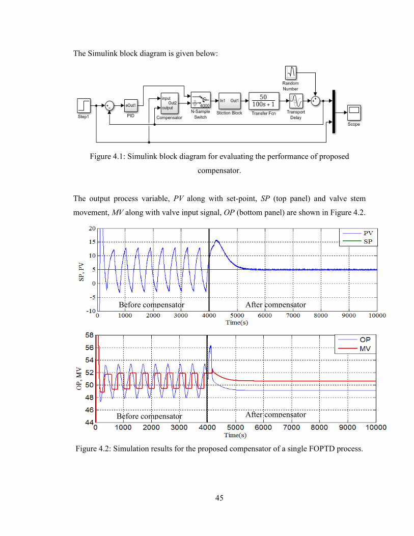
45

The Simulink block diagram is given below:

Figure 4.1: Simulink block diagram for evaluating the performance of proposed

compensator.

The output process variable, PV along with set-point, SP (top panel) and valve stem

movement, MV along with valve input signal, OP (bottom panel) are shown in Figure 4.2.

Figure 4.2: Simulation results for the proposed compensator of a single FOPTD process.

Before compensator After compensator

After compensator Before compensator

46

Figure 4.2 shows that the process variable, PV was oscillatory up to 4000 s due to valve

stiction. At 4000 s, the compensator was started and the compensator could eliminate the

oscillations completely in about 1200 s time. Therefore, it can be said that the proposed

compensator can mitigate the stiction effect satisfactorily by reducing process oscillation

as well as valve stem movements.

4.2 Evaluation of the Performance of the Compensator for different FOPTD process

The proposed method was also evaluated for different First Order Plus Time Delay

(FOPTD) processes. The general model for FOPTD processes can be written as:

(4.3)

Where, is process gain, is time constant and is time delay. The process gain ,

time constant and time delay were varied in the range of [1:5:51], [1:10:201] and

[0:3:21], respectively. These combinations produced 1848 different FOPTD processes.

The controller parameters were calculated based on IMC rules for different processes.

The parameters of the proposed compensator were kept same as before. Only the

detuning parameter α was different for every model which was dependent on the process

parameters. Every process models were run for 10000 s and the compensator started at

4000 s for each case. For the sake of brevity, it is not possible to show all results. Some

compensation results are shown in Figure 4.3 for different FOPTD processes.

Figure 4.3 (a): Sample results for different FOPTD model.

47

Figure 4.3 (b): Sample results for different FOPTD model.

Figure 4.3 shows that the process output is oscillatory before starting the compensator.

After the compensator was switched on at 4000 s, the oscillations in the process output,

PV were gone completely. Therefore, it can be said that the proposed compensator works

satisfactorily for different FOPTD processes.

48

4.3 Evaluation of the Compensator Performance for Different Perturbations

The proposed compensation scheme was applied for different scenarios on the same

process and the controller described by Equation 4.1 and 4.2, respectively. Stiction was

introduced by using the widely used Choudhury et al., (2005) stiction model. The stiction

parameters (S=5, J=3) were used for first three cases. The compensator was evaluated for

four cases such as 1) set-point tracking 2) disturbance rejection 3) various noise level and

4) varying amount of stiction.

4.3.1 Set Point Tracking

The proposed compensator model was tested to check its performance during set-point

tracking control. The compensator was triggered ON at time instant, t=4000 s. The top

panel in Figure 4.4 shows that the oscillations have been eliminated and process variable

can track the different set point changes successfully. The bottom panel shows that there

is no excessive valve movement and the number of valve reversals is also minimum.

Figure 4.4: Stiction compensation for set-point tracking.

Before compensator

Before compensator

After compensator

After compensator

49

4.3.2 Disturbance Rejection

Any step disturbance tends to deviate the process output from its set point. It is desirable

to remove the effect of disturbance within a short time. The compensator was applied at

t=4000 s. It could eliminate the oscillation and bring the process at steady state around

4800 s. Then a unit step type disturbance was applied at 7000 s. The proposed

compensator could eliminate the step disturbance effectively within a short period of

time. The bottom panel of Figure 4.5 shows that the valve stem returns quickly at the

desired steady state position. Therefore, it can be said that step type disturbance could be

eliminated effectively by the proposed compensator.

Figure 4.5: Results for proposed compensator when a step disturbance is added at 7000 s.

After compensator Before compensator

After compensator Before compensator

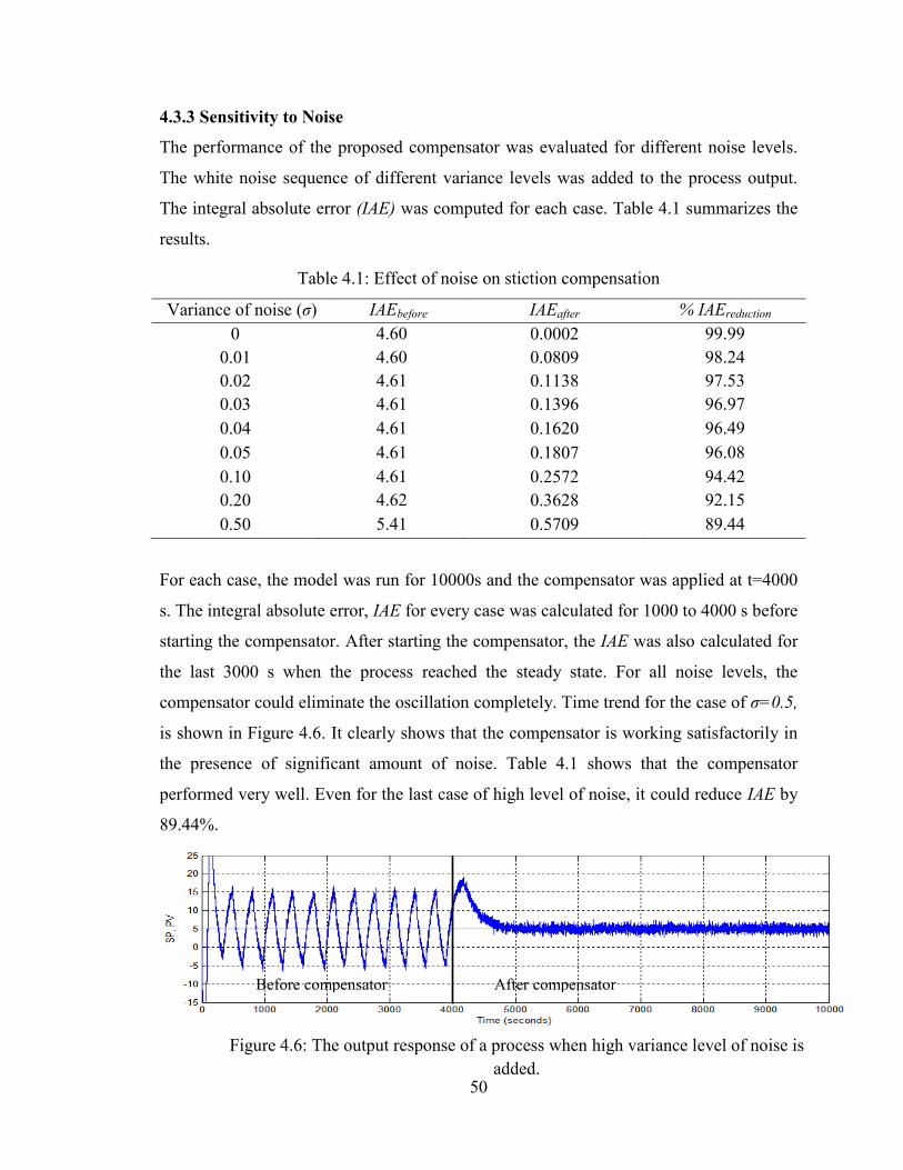
50

4.3.3 Sensitivity to Noise

The performance of the proposed compensator was evaluated for different noise levels.

The white noise sequence of different variance levels was added to the process output.

The integral absolute error (IAE) was computed for each case. Table 4.1 summarizes the

results.

Table 4.1: Effect of noise on stiction compensation

Variance of noise (σ) IAEbefore IAEafter % IAEreduction

0 4.60 0.0002 99.99 0.01 4.60 0.0809 98.24 0.02 4.61 0.1138 97.53 0.03 4.61 0.1396 96.97 0.04 4.61 0.1620 96.49 0.05 4.61 0.1807 96.08 0.10 4.61 0.2572 94.42 0.20 4.62 0.3628 92.15 0.50 5.41 0.5709 89.44

For each case, the model was run for 10000s and the compensator was applied at t=4000

s. The integral absolute error, IAE for every case was calculated for 1000 to 4000 s before

starting the compensator. After starting the compensator, the IAE was also calculated for

the last 3000 s when the process reached the steady state. For all noise levels, the

compensator could eliminate the oscillation completely. Time trend for the case of σ=0.5,

is shown in Figure 4.6. It clearly shows that the compensator is working satisfactorily in

the presence of significant amount of noise. Table 4.1 shows that the compensator

performed very well. Even for the last case of high level of noise, it could reduce IAE by

89.44%.

Before compensator After compensator

Figure 4.6: The output response of a process when high variance level of noise is added.

51

4.3.4 Sensitivity to Extent of Stiction

The compensator developed in this study does not require the knowledge of stiction

parameters. The measurement of stiction parameters is cumbersome. The sticband plus

deadband for upward and downward direction of valve travel could be different. A

modified version stiction model appeared in Choudhury et al., (2005) was used to

simulate asymmetric stiction. The modified version was capable of specifying different

amount of sticband plus deadband in the upward and downward direction of valve travel.

The deadband plus sticband parameter, S is denoted as 'SU' for upward and as 'SD' for

downward direction. The other parameter slip jump is denoted by, J. Various stiction

cases are simulated for stiction parameters listed in the first column of Table 4.2. The

performance of the proposed compensator for these different cases were evaluated by

calculating IAEbefore from 1000 s to 4000 s and IAEafter from 7000 s to 10000 s. The

compensator performed well in all cases as shown in Table 4.2.

Table-4.2: Impact of stiction parameters on stiction compensation

SU,SD,J

Detuning parameter,

α Time trend IAEbefore IAEafter

3,3,3 10

4.05 0.081

7,5,3 10

5.70 0.080

10,6,4 40

7.45 0.083

10,8,6 10

10.20 0.084

52

4.4 Chapter Summary

The performance of the proposed compensator has been evaluated in this chapter. The

proposed compensator can mitigate stiction effect satisfactorily. It can track set point and

reject disturbance for various combination of FOPTD processes. The performance of the

proposed compensator under various perturbations has also been discussed.

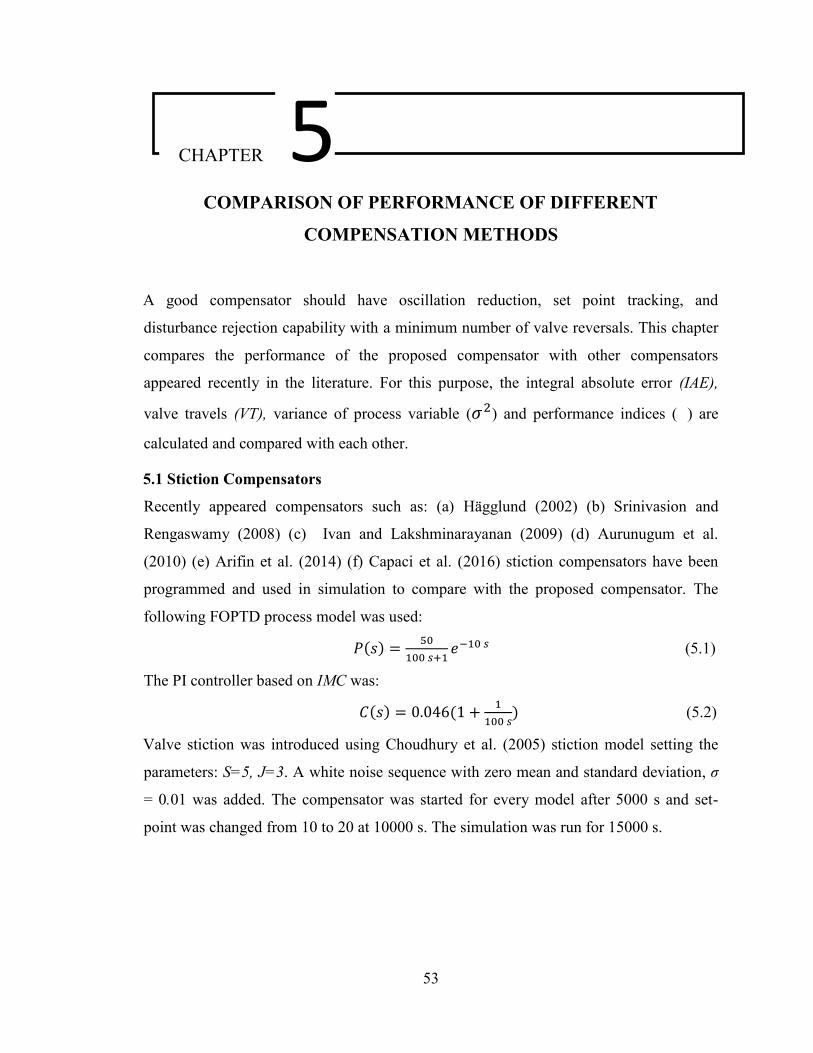
53

COMPARISON OF PERFORMANCE OF DIFFERENT

COMPENSATION METHODS

A good compensator should have oscillation reduction, set point tracking, and

disturbance rejection capability with a minimum number of valve reversals. This chapter

compares the performance of the proposed compensator with other compensators

appeared recently in the literature. For this purpose, the integral absolute error (IAE),

valve travels (VT), variance of process variable ( ) and performance indices ( ) are

calculated and compared with each other.

5.1 Stiction Compensators

Recently appeared compensators such as: (a) Hägglund (2002) (b) Srinivasion and

Rengaswamy (2008) (c) Ivan and Lakshminarayanan (2009) (d) Aurunugum et al.

(2010) (e) Arifin et al. (2014) (f) Capaci et al. (2016) stiction compensators have been

programmed and used in simulation to compare with the proposed compensator. The

following FOPTD process model was used:

(5.1)

The PI controller based on IMC was:

(5.2)

Valve stiction was introduced using Choudhury et al. (2005) stiction model setting the

parameters: S=5, J=3. A white noise sequence with zero mean and standard deviation, σ

= 0.01 was added. The compensator was started for every model after 5000 s and set-

point was changed from 10 to 20 at 10000 s. The simulation was run for 15000 s.

5 CHAPTER

54

5.2 Comparison of Trend Analysis

The trends of process variable, PV and set-point, SP for different compensator models are

shown in Figure 5.1. As can be seen from this figure, all compensator are able to reduce

the process oscillations and track the set-point successfully. However all of them except

Capaci et al. (2016) and the proposed compensator could only reduce the amplitude of

oscillations at the price of increasing the frequency of oscillations. As a result, the

number of valve reversals has been increased significantly.

The Capaci et al. (2016) model could reduce the oscillations successfully but oscillation

returns for a certain period of time for a set-point change at 10000s. But for the proposed

compensator, oscillations have not come back for the set-point changes. Thus, the

proposed compensator outperforms all other compensator appeared in the literature.

Figure 5.1 (a): Response curve of output process variable, PV and set point, SP for

different compensator model.

Before compensator After compensator

Before compensator

Before compensator

Before compensator

After compensator

After compensator

After compensator

0 5000 Time(s) 10000 15000 a) Haggland (2002)

SP, P

V

-10

1

0

30

0 5000 Time(s) 10000 15000 b) Srinivasion and Rengaswamy (2008)

SP, P

V

-10

1

0

30

0 5000 Time(s) 10000 15000 c) Ivan and Lakshminarayanan (2009)

SP, P

V

-10

1

0

30

0 5000 Time(s) 10000 15000 d) Arununugum et al. (2010)

SP, P

V

-10

1

0

30

55

The valve stem position, MV along with controller output, OP are plotted in Figure 5.2.

From this Figure, it is clearly shown that the first five methods have increased the valve

movements and caused a significant increase in valve reversals after the compensator was

switched on at 5000 s. This will certainly reduce the longitivity of control valve. A good

compensator is expected to mitigate stiction effect and reduces process oscillation

without increasing the number of valve revarsals. Figure 5.1 and 5.2 show that the only

last two method namely Capaci et al. (2016) and the proposed method can successfully

track set-point and reduce oscillation of process variables without increasing number of

valve reversals.

Figure 5.1 (b): Response curve of output process variable, PV and set point, SP for different

compensator model.

Before compensator

Before compensator

Before compensator

After compensator

After compensator

After compensator

0 5000 Time(s) 10000 15000 e) Arifin et al. (2014)

SP, P

V

-10

1

0

30

0 5000 Time(s) 10000 15000 f) Capaci et al. (2016)

0 5000 Time(s) 10000 15000 g) Proposed Model

SP, P

V

-10

1

0

30

SP, P

V

-10

1

0

30

56

Before compensator

Before compensator

Before compensator

Before compensator

Before compensator

Before compensator

Before compensator

After compensator

After compensator

After compensator

After compensator

After compensator

After compensator

After compensator

0 5000 Time(s) 10000 15000 a) Haggland (2002)

0 5000 Time(s) 10000 15000 b) Srinivasion and Rengaswamy (2008)

0 5000 Time(s) 10000 15000 c) Ivan and Lakshminarayanan (2009)

0 5000 Time(s) 10000 15000 d) Arununugum et al. (2010)

0 5000 Time(s) 10000 15000 e) Arifin et al. (2014)

0 5000 Time(s) 10000 15000 f) Capaci et al., (2016)

0 5000 Time(s) 10000 15000 g) Proposed Model

OP,

MV

30

50

7

0

OP,

MV

30

50

7

0

OP,

MV

30

50

7

0

OP,

MV

30

50

7

0

OP,

MV

30

50

7

0

OP,

MV

30

50

7

0

OP,

MV

30

5

0

70

Figure 5.2: Response curve of valve position, MV and controller output, OP for different compensator model.

57

5.3 Comparison of Performance

In this section, the performance of different compensators are quantified and compared

with each other. The performance can be quantified using the integral absolute error, IAE,

process variable variance, and valve travel, VT. Smaller values of IAE and mean

that compensator can reduce process oscillation, track set-point and reject disturbance

satisfactorily. The valve reversals can be analyzed by calculating valve travels, VT.

Minimum number of valve reversals results smaller VT. So a good compensator have

minimum IAE, and VT. These parameters are calculated as follows:

(5.3)

(5.4)

(5.5)

Where, e (t) is the difference between set-point and process variable and x(t) represents

the valve position at time t, is the mean value of process variable and N is the total

number of data points.

The compensator for every model was activated at 5001 s. The IAE, and VT before

compensator were calculated using data for 1000 s to 5000 s and those values after

compensator were calculated using data for 6000 s to 10000 s. The values of IAE before

and after the compensator are shown in Table-5.1. The percent decrease of integral

absolute error, IAE is also shown in the right-most column of this Table. The proposed

method has the minimum IAE among all compensators. The proposed compensator could

reduce IAE by 97.2%, which is maximum among all of them.

58

Table-5.1: Integral Absolute Error, IAE data for different compensator model.

Name of the Model IAEbefore IAEafter % decrease of

IAE

Hägglund (2002)

4.657

1.525 67.3

Srinivasion and Rengaswamy (2008) 1.316 71.7

Ivan and Lakshminarayanan (2009) 2.118 54.5

Aurunugum et al. (2010) 0.854 81.7

Arifin et al. (2014) 2.268 51.3

Capaci et al. (2016) 0.407 91.3

Proposed Compensator 0.1303 97.2

The minimum process variable variance indicates the smaller oscillation in the output

process variable. As shown in Table 5.2, before the compensator was started, the PV

variance was 27.193 for all cases. All of the compensators can reduce the oscillations but

the proposed compensator outperforms all other methods.

Table-5.2: Variance of output process variable, data for different compensator model.

Name of the Model before after % decrease of

Hägglund (2002)

27.193

2.873 89.4 Srinivasion and Rengaswamy (2008) 2.318 91.5 Ivan and Lakshminarayanan (2009) 6.016 77.9 Aurunugum et al., (2010) 0.969 96.4 Arifin et al. (2014) 6.496 76.1 Capaci et al. (2016) 0.436 98.4 Proposed Compensator 0.044 99.8

Depending on the valve stem position, valve travel, VT was measured. Actually VT

cannot be measured in actual industrial process plants because MV data is not generally

available. Thus the measurement of VT is possible for simulation study to evaluate the

performance of the compensator. The quantified results of VT for different compensator

59

are summarized in Table- 5.3. The last column shows the percentage change of VT before

and after compensator was applied. Actually, VT has increased after starting the

compensator than it was before for most cases. The last column of Table- 5.3 shows that

only the proposed and Capaci et al. (2016) compensator could reduce the valve travels. In

these two methods, valve reached to a steady state position quickly after starting the

compensator. Then they could reduce the valve travels by 95% and 76% respectively,

whereas other compensators have increased the valve travels in manifolds. Excessive

valve movements reduce the longevity of the valve. So, the implementation of these

compensators in real industry would damage the control valve within a short period of

time. The implementation of the proposed compensator in real industry would be

beneficial because it can mitigate the stiction effect without increasing the valve stem

movements.

Table-5.3: Valve Travel, VT, data for different compensator models.

Name of the Model VTbefore VTafter % change of VT

Hägglund (2002)

7.561

356.4 4595

Srinivasion and Rengaswamy (2008) 124.5 1547

Ivan and Lakshminarayanan (2009) 425.3 5524

Aurunugum et al. (2010) 69.30 817

Arifin et al. (2014) 473.8 6166

Capaci et al. (2016) 1.799 -76

Proposed Compensator 0.351 -95

The results in Table 5.1, 5.2, 5.3 show that the last two methods are the best stiction

compensators among the widely used compensation method available in literature.

Between the last two, the proposed method gives better results than the Capaci et al.

(2016) method.

5.4 Comparison of the Proposed Method and Capaci et al. (2016) Method.

The analysis in section 5.1, 5.2 and 5.3 show that the proposed compensator and Capaci

et al. (2016) method outperforms all other available compensation methods. The

performances of both compensators with respective to set-point tracking, IAE, and VT

60

are very close. However, the proposed compensator performs better than the Capaci et al.

(2016) method. The performances of these two methods are investigated more elaborately

below.

5.4.1 Disturbance Rejection Capability

Disturbance is very common for every process industry. A good compensator should

have quicker disturbance rejection capability. A unit step disturbance was applied at

10000s for two different compensator models applied on the same process model

described by Equation 5.1. The trends of the process variables for the two cases are

shown in Figure 5.3 and 5.4. In Figure 5.3 (Capaci et al., 2016), oscillation returns and

stays for about 1000 s before the disturbance can be eliminated. One the other hand, the

proposed compensator can quickly reject the unit step disturbance within a short period

of time as shown in Figure 5.4. It is noteworthy to mention that when compensator was

switched on at 5000 s, the proposed compensator could remove oscillation earlier and

perform better than Capaci et al. (2016). (See Figure 5.3 and 5.4)

After compensator Before compensator

After compensator Before compensator

0 5000 Time (s) 10000 15000

Figure 5.3: Unit step disturbance rejection capability for Capaci et al. (2016) method.

SP, P

V

-10

0

10

20

3

0

0 5000 Time (s) 10000 15000

Figure 5.4: Unit step disturbance rejection capability for proposed compensator method.

SP, P

V

-10

0

10

20

3

0

61

5.4.2 Uncertainty in Stiction Amount

The Capaci et al. (2016) method is strictly dependent on the estimation of stiction

parameter. Accurate stiction detection is a priori in their work. Incorrect detection of

stiction parameters can produce wrong results. It can reduce the oscillation but cannot

track the set point. As shown in Figure 5.5, there is an offset between PV and SP.

Figure 5.5: Process response curve of unknown stiction parameter for Capaci et al. (2016)

method.

On the other hand, for the proposed compensator, there is no requirement of knowing

values of stiction parameters. As shown in Figure 5.6, the proposed compensator can

remove oscillations and at the same time, can track the set-point accurately.

Figure 5.6: Process response curve for proposed method for the case of unknown stiction

parameters.

Accurate measurement of stiction parameters for a real industrial plant are difficult.

Therefore, the implementation of the Capaci et al. (2016) compensation technique in real

plant will be cumbersome. The proposed compensator is simple and can be implemented

in a real plant without knowing the extent of stiction in control valve.

Before compensator After compensator

After compensator Before compensator

62

5.4.3 Non-Homogeneous Stiction Case

The Capaci et al. (2016) compensation technique works only for constant parameter

stiction model. It cannot be used for the case of non-homogeneous stiction model. Non-

homogeneous stiction means that the values of stickband plus deadband for upward, SU

and downward, SD direction of valve travel could be different. The proposed

compensator can also work for non-homogeneous stiction parameters. A sample results

for non-homogeneous stiction parameters is shown in Figure 5.7. A modified version of

stiction model (SU=7,SD=5,J=3) appeared in Choudhury et al. (2005) was used to

evaluate the performance of compensator for non-homogeneous cases of stiction.

Figure 5.7: Simulation results of proposed model for non-homogeneous stiction

parameters.

5.4 Chapter Summary

In this chapter, the performances of the available stiction compensators along with the

proposed compensator are compared. The process output trends, the integral absolute

error, process variable variance and the valve travel values were compared for seven

different compensation methods. It was found that the proposed compensator

outperforms all other compensation methods available in the literature.

63

EXPERIMENTAL EVALUATION OF THE

PROPOSED COMPENSATION TECHNIQUE

The industrial chemical processes generally contain a thousands of process control loops.

The product quality greatly depends on performance of such control loops. But control

loop suffers from poor performance due to nonlinearity or oscillation of the final control

element, control valve. Among the many types of non-linearities in control valves,

stiction is the most common in the process industry. Compensation of control valve

stiction thus has become an important topic of research and development. This chapter

discusses the experimental evaluation of the proposed stiction compensation method

applied to a level control loop of a computer interfaced pilot plant located in the process

control laboratory of Chemical Engineering Department, BUET

6.1 Description of the Plant

The pilot plant set up located in Chemical Engineering Laboratory, BUET consists of

four tank level plus temperature control system. The small tank with a level control loop

was used to carry out the experiment. A photograph of experimental set-up is shown in

Figure 6.1 and a schematic diagram of the level control loop is shown in Figure 6.2.

Figure 6.1: Experimental set-up of the water level control system.

6 CHAPTER

64

Figure 6.2: Schematic diagram of the water level control system.

A brief description of the various components of the system is given below:

i. Small Tanks

A small tank of cylindrical shape is located in the pilot plant. The tank was attached with

a stand. Material of construction of the tank is glass. It was 2 ft long with a 4 inch in

diameter.

ii. Pneumatic Control Valve

The pneumatic control valve in the pilot plant is fail close type. Material of construction

of the valve is SS, internal threaded. Size of each valve is 1/2 inch in diameter.

iii. Transmitter

There is a level transmitter with the tank. The transmitter is of Model 1151 Smart

Pressure Transmitter manufactured by Fisher-Rosemount Inc.

iv. Manual Valves

There are two types of manual valves in the set-up. These are ball valves and needle

valves. Material of construction for all type of valves is SS, internal threaded. Size of the

needle valves is 1/2 inch and ball valves are of 1 inch, 1/2 inch and 1/4 inch.

65

v. Compressor

A centrifugal compressor is used to supply instrument air to the pilot plant. Compressed

air is necessary to operate the pneumatic control valve. The compressor was used to

supply the required compressed air to the valve.

vi. Water Supply Line

All pipe line for transporting water are made of SS. The size of main pipe line is 1/2 inch

in diameter, Schedule 10 and the size of the lines that goes to the transmitters is 1/4 inch

diameter, Schedule 10.

vii. Instrumental Air Supply

From the instrument air header, air is supplied to operate the pneumatic control valves.

Minimum air pressure required for the system is 4 bar. The material of construction of the

header is SS. Size is 1 inch, Schedule 10. 6 mm PVC tubes are used as pneumatic cables.

The pilot plant has SISO (single input single output) configuration containing a level

control loop. Water was coming through the inlet pipeline of the tank. There was a flow

control valve named LCV02 in the water inlet line. The process objective was to maintain

the level of the tank at a desired value. To maintain the level of the tank, the inlet flow

rate of water must be regulated using the control valve LCV02. Level of the tank was

measured and transmitted using a level sensor LTS01. For automatic control

configuration, this would make feedback control loop for the process.

The process was interfaced with MATLAB Simulink software through OPC server

connectivity.

The block diagram is shown in Figure 6.3.

Figure 6.3: Simulink block diagram of a level control feedback loop.

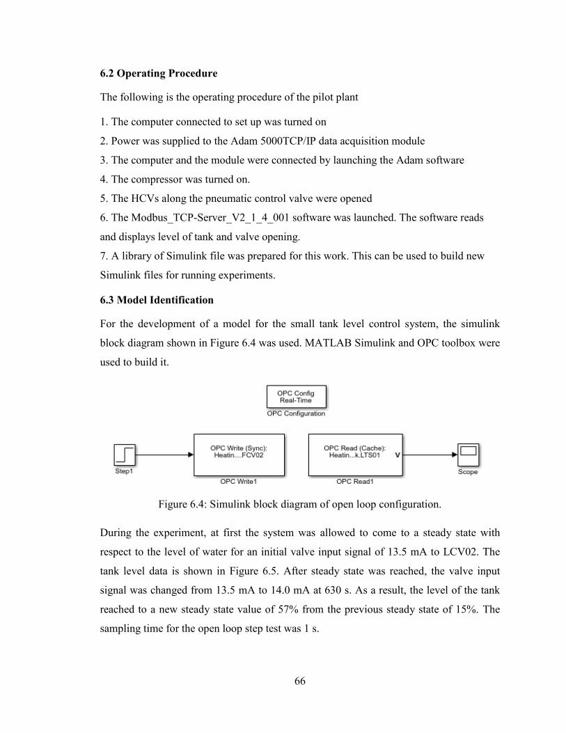
66

6.2 Operating Procedure

The following is the operating procedure of the pilot plant

1. The computer connected to set up was turned on

2. Power was supplied to the Adam 5000TCP/IP data acquisition module

3. The computer and the module were connected by launching the Adam software

4. The compressor was turned on.

5. The HCVs along the pneumatic control valve were opened

6. The Modbus_TCP-Server_V2_1_4_001 software was launched. The software reads

and displays level of tank and valve opening.

7. A library of Simulink file was prepared for this work. This can be used to build new

Simulink files for running experiments.

6.3 Model Identification

For the development of a model for the small tank level control system, the simulink

block diagram shown in Figure 6.4 was used. MATLAB Simulink and OPC toolbox were

used to build it.

Figure 6.4: Simulink block diagram of open loop configuration.

During the experiment, at first the system was allowed to come to a steady state with

respect to the level of water for an initial valve input signal of 13.5 mA to LCV02. The

tank level data is shown in Figure 6.5. After steady state was reached, the valve input

signal was changed from 13.5 mA to 14.0 mA at 630 s. As a result, the level of the tank

reached to a new steady state value of 57% from the previous steady state of 15%. The

sampling time for the open loop step test was 1 s.

67

Figure 6.5: The open loop response curve for the pilot plant.

Figure 6.5 shows that it can be modeled using a First Order Plus Time Delay (FOPTD)

model. The general transfer function for such a process is:

(6.1)

The model parameter can be calculated as follows,

Process gain,

(6.2)

From Figure 6.5,

The time delay, is the time lag between input and output response. From Figure 6, it

can be estimated as:

= (640-630) s= 10 s

For a first order process, time constant, is the time when the system reaches 63.2% of

its ultimate value. The 63.2% of the ultimate response is 15+ (57-15) × 0.632 = 41.54%

level for this system. This has been shown in Figure 6.5. The corresponding time to reach

41.54% value for the level can be read from the x-axis of Figure 6.5, which is 820 s.

Δy=42%

10s

Δx=0.5mA

=180

41.54%

68

Therefore,

= (820- -640) s = (820-10-630) s = 180 s

Thus from the above open loop test, the transfer function of the process was obtained as:

(6.3)

6.4 PI(D) Controller Design

The controller parameters, KC and were calculated using the Internal Model Control (IMC) rules. The controller parameters were obtained by fine tuning the PI(D) controller after applying it to the process without any compensator and without any stiction.

The final controller settings were obtained as:

(6.4)

The output process variable along with set-point for the final controller settings is shown

in Figure 6.6. In this figure, the set-point was changed from 20% to 30% at 1000 s and

30% to 40% at 2000 s. The process output could track the set-point successfully for all

cases without producing any oscillations. So, it can be said that the controller settings in

Equation 6.4 is a good controller for this process.

Figure 6.6: The process output results for the non-sticky condition using the final

controller settings.

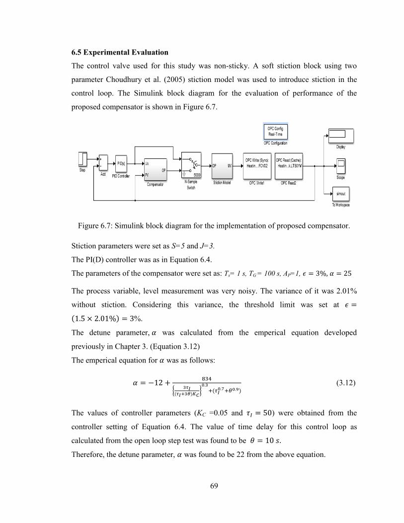
69

6.5 Experimental Evaluation

The control valve used for this study was non-sticky. A soft stiction block using two

parameter Choudhury et al. (2005) stiction model was used to introduce stiction in the

control loop. The Simulink block diagram for the evaluation of performance of the

proposed compensator is shown in Figure 6.7.

Figure 6.7: Simulink block diagram for the implementation of proposed compensator.

Stiction parameters were set as S=5 and J=3.

The PI(D) controller was as in Equation 6.4.

The parameters of the compensator were set as: Ts= 1 s, TG = 100 s, AP=1,

The process variable, level measurement was very noisy. The variance of it was 2.01%

without stiction. Considering this variance, the threshold limit was set at

%.

The detune parameter, was calculated from the emperical equation developed

previously in Chapter 3. (Equation 3.12)

The emperical equation for was as follows:

(3.12)

The values of controller parameters (KC =0.05 and ) were obtained from the

controller setting of Equation 6.4. The value of time delay for this control loop as

calculated from the open loop step test was found to be

Therefore, the detune parameter, was found to be 22 from the above equation.

70

Figure 6.8 shows the results of the implementation of stiction compensation scheme. As

shown in Figure 6.8, from 0 to 1000 s, there was no stiction compensation. The lower

panel of this Figure shows that the valve stem moves ups and down in between 61% to

67% as well as controller output oscillates from about 60% to 68% due to valve stiction.

Therefore, the level of water in the tank oscillates from 20% to 40%. At 1000s, the

proposed compensation scheme was applied. After starting the compensator, the valve

became almost stack at desired position till the set point changes. The valve stem would

stack again at new desired position for corresponding set-point changes. So, the

compensator could remove the oscillation of the output process variables satisfactorily.

The set-point was changed from 30% to 40% at 3000 s, 40% to 50% at 6000 s and 50%

to 60% at 8500 s. The compensation quality was not deteriorated due to change in set-

point. Therefore, the proposed compensator could track the set-point change and could

also remove oscillation completely.

Figure 6.8: Experimental results of the proposed compensator.

Before Compensator

After Compensator

Before Compensator

After Compensator

71

Three cases namely 1) Non-sticky valve 2) Stiction without compensator and 3) Stiction

with compensator are considered for further analysis. The variance of the process

variable for three cases was calculated and listed in Table 6.1. For non-sticky valve, the

process variable was mainly noisy and does not show any oscillation. This results in a

variance of 2.01% as shown in the top row in Table 6.1. For the case of sticky valve, the

process variable was oscillatory due to stiction before starting the compensator.

Consequently, the variance of the process variable was very high. It was 58.72% as

shown in the middle row of Table 6.1. After the compensator was switched on, it

eliminated the oscillation completely and the process variable has almost returned to the

previous state of non-sticky valve case. The variance of the process variable is almost

same as the variance of the process variable for the case of non-sticky valve. Therefore, it

can be said that the proposed compensator was able to mitigate the stiction effect quite

effectively.

Table 6.1: Process Variable variance for different conditions.

Sl. No. Conditions Time trend Process variable variance

1 Non-Sticky

valve

2.01

2

Stiction

without

compensator

58.72

3 Stiction with

compensator

2.11

72

6.6 Chapter Summary

This chapter provides a description of the tank level control set-up located at the process

control laboratory of the Department of Chemical Engineering, BUET. A brief operating

procedure for this system is provided. This chapter shows the identification result of the

FOPTD process. It also evaluates the performance of the proposed compensator through

experimental validation.

73

CONCLUSION AND RECOMMENDATION

7.1 Conclusions

Chemical industries are very sophisticated and consist of hundreds or thousands of

control valves. Stiction in control valve produces oscillation in process variables and

reduces the product quality. If a control valve is found to be sticky, the permanent

solution is to send it to workshop for maintenance. In most cases, it cannot be done

without shutting down the plant. Therefore, it is a challenging task to develop a

compensator to mitigate stiction effects while the plant is running. This thesis has

developed such a stiction compensator. The main contribution of this study can be

summarized as follows:

1. A new stiction compensator has been developed to mitigate the adverse impact of

valve stiction. It can be applied online without stopping the process plant.

2. Methods for estimating the parameters of the proposed stiction compensator have

also been developed.

3. The performance of the proposed compensator has been extensively evaluated for

different First Order Plus Time Delay (FOPTD) processes through simulation

study.

4. The performance of the proposed compensator was compared with other

compensators available in the literature such as Hägglund (2002), Srinivasion and

Rengaswamy (2008), Ivan and Lakshminarayanan (2009), Aurunugum et al.

(2010), Arifin et al. (2014), Capaci et al. (2016). It was found that the proposed

compensator outperforms all of them.

5. Finally, the proposed compensator was applied to a level control loop in a pilot

plant experimental set up and was found to be successful in removing oscillation

due to valve stiction.

7 CHAPTER

74

The developed compensator has the desired capability of minimizing the process

variability with a minimum number of valve reversals. It has good set-point tracking and

disturbance rejection properties. The compensation scheme is simple yet powerful. It

requires minimum process knowledge. It would not be difficult to implement it in process

plants.

7.2 Recommendations for Future Work

There is a scope of improvement and extension of this research work. The following

recommendations show some directions to future work.

1. The proposed compensator was developed based on FOPTD process. Though

most real processes can be approximated using FOPTD processes, the

compensator should be evaluated and modified as necessary for other higher order

processes and non-linear processes.

2. The proposed compensator should be applied to a real industrial processes using

DCS system.

3. Currently, all available compensators require user-defined parameters based on

the process. New research can be directed to automate this process so that the user

requires minimum effort to use a compensator.

75

REFERENCES

[1] Arifin, B. M. S., Munaro, C. J., Angarita, O. F. B., Cypriano, M. V. G. and Shah, S. L.

(2018) ‘Actuator stiction compensation via variable amplitude pulses’, ISA Transactions.

ISA, pp. 1–10.

[2] Arifin, B. M. S., Munaro, C. J. and Shah, S. L. (2014) ‘A Model Free Approach for

Online Stiction’, in The International Federation of Automatic Control. Cape Town,

South Africa, pp. 5957–5962.

[3] Arumugam, S., Panda, R. C. and Velappan, V. (2014) ‘A simple method for

compensating stiction nonlinearity in oscillating control loops’, International Journal of

Engineering and Technology, 6(4), pp. 1846–1855.

[4] Bialkowski, W. L. (1993) ‘Dreams versus reality: a view from both sides of the gap:

manufacturing excellence with come only through engineering excellence’, Pulp &

Paper Canada, 94, pp. 19–27.

[5] Capaci, R. B. di, Scali, C. and Huang, B. (2016) ‘A Revised Technique of Stiction

Compensation for Control Valves’, in IFAC-PapersOnLine. Trondheim, Norway, pp.

1038–1043.

[6] Choudhury, A. A. S., Shah, S. L. and Thornhill, N. F. (2008) Diagnosis of process

nonlinearities and valve stiction: data driven approaches. Berlin Heidelberg: Springer.

[7] Choudhury, M. A. A. S, Thornhill, N. F. and Shah, S. L. (2005) ‘Modelling valve

stiction’, Control Engineering Practice, 13(5), pp. 641–658.

[8] Desborough, L., Nordh, P. and Miller, R. (2001) ‘Control system reliability: process out

of control’, Industrial Computing, 8, pp. 52–55.

[9] De Souza, M. A., Munaro, C. J. and Munareto, S. (2012) ‘Novel model-free approach for

stiction compensation in control valves’, Industrial and Engineering Chemistry Research,

51(25), pp. 8465–8476.

[10] Farenzena, M. and Trierweiler, J. O. (2010) ‘Modified PI controller for stiction

compensation’, in IFAC Proceedings Volumes (IFAC-PapersOnline). IFAC, pp. 799–

804.

[11] Hägglund, T. (2002) ‘A friction compensator for pneumatic control valves’, Journal of

Process Control, 12(8), pp. 897–904.

76

[12] He, Q. P., Pottmann, J. W. M. and Qin, J. S. (2007) ‘A Curve Fitting Method for

Detecting Valve Stiction in Oscillating Control Loops’, Industrial & Engineering

Chemistry Research, 46(13).

[13] ISA Committee SP51 (1979), Process instrumentation terminology,Instrument Society of

America.

[14] Ivan, L. Z. X. and Lakshminarayanan, S. (2009) ‘A new unified approach to valve

stiction quantification and compensation’, Industrial and Engineering Chemistry

Research, 48(7), pp. 3474–3483.

[15] Karthiga, D. and Kalaivani S. (2012) ‘A new stiction compensation method in pneumatic

control valves’, International Journal of Electronics and Computer Science Engineering,

1(4), pp. 2604–2612.

[16] Li, X., Chen, S. L., Teo, C. S., Tan, K. K., and Lee, T. H. (2014) ‘Revised binary tree

data-driven model for valve stiction’, in Conference Proceedings - IEEE International

Conference on Systems, Man and Cybernetics, pp. 3890–3895.

[17] Marco, M. A., Munaro, C. J. and Munareto, S. (2012) ‘Improved stiction compensation in

pneumatic control valves’, Computers and Chemical Engineering. Elsevier Ltd, 38, pp.

106–114.

[18] Sivagamasundari, S. and Sivakumar, D. (2013) ‘A New Methodology to Compensate

Stiction in Pneumatic Control Valves’, International Journal of Soft Computing and

Engineering, 2(6), pp. 480–484.

[19] Srinivasan, R. and Rengaswamy, R. (2008) ‘Approaches for efficient stiction

compensation in process control valves’, Computers and Chemical Engineering, 32(1–2),

pp. 218–229.

[20] Wang, T., Xie, L., Tan, F., and Su, H. (2015) ‘A new implementation of open loop two

move compensation method for oscillation caused by control valve stiction’, in IFIC

ADCHEM. Whistler, BC, Canada, pp. 433–438.

77

Appendix-A

Characteristics curve of small tank inlet control valve (FCV02) in Process Control

Laboratory of Chemical Engineering Department, BUET

78

Appendix-B

Matlab Algorithm of Proposed Stiction Compensator

function y=CompensationModel(x)

pid=x(4);%signal from controller

detuner=x(1);%detune parameter

error=x(3);%error

diff=x(2);%acceptable deviation

pulse=x(5);%signal from pulse generator

TG=x(6);%for countng total time

TG=TG+1;

if abs(error)<=diff;%check whether the control is acceptable or not

TG=0;

valve=pid/(detuner);% reduce the aggressiveness of the controller

else

if TG<100 && error>diff

valve=(pid/detuner)-pulse;

elseif TG<100 && error<diff

valve=(pid/detuner)+pulse;

else

valve=pid/(detuner);

end

end

y=[valve TG];

79

Appendix-C

Matlab Algorithm for Compensator Initialization

function Y = integrator(X) source = X(1); integrated_source = X(2); time = X(3); source_sum = X(4); cache = X(5); swtime = X(6); a=X(7); if( time<=(swtime - 1)) source_sum = source_sum + source; end

final_output = integrated_source; if (time==swtime) final_output = source_sum*a/swtime; cache = integrated_source; elseif(time>swtime) final_output = (final_output - cache + source_sum*a/swtime); end

tp = time + 1;

Y = [final_output tp source_sum cache]; end

80

Appendix-D

Matlab Algorithm to find detune parameter

clc clear all close all Ts=1; e=0.5; m=[]; q=0; swtime=4000;% the compensator start for k=1:5:51 % Process gain for t=1:10:201 % Process time constant for d=0:3:21 % Time delay p=0; for a=1:0.5:200; % detune parameter sim('Simmodel'); % MatLab Simulink p=p+1; w=(sum(IAE(:,1)))/3000; A(p) = a m(p)=w; end index1=find (m==min(m));

for ID = 1:length(index1) q=q+1; min_a = A(index1(ID)); n4(q,1:5)=[k t d min_a min(m)] break; end end end end

81

Appendix-E

Matlab Algorithm to plot Compensation Results for

Different FOPTD Process clc clear all close all Ts=1; e=0.5; q=0; swtime=4000; j=0; load IAEVT for i=1:length(IAEVT)

if (IAEVT(i,5)<0.1 && IAEVT(i,6)>0) if j>=6 j=0; figure end k=IAEVT(i,1); t=IAEVT(i,2); d=IAEVT(i,3); j=j+1; sim('Simmodel_witheq')

subplot(6,2,j) plot(pv) grid on axis([0,10000,-10,20]) pp=['Kp=', num2str(k),',Tau=', num2str(t), ',Theta=', num2str(d)] title(num2str(pp)) xlabel('Time(s)') ylabel('Response') elseif (IAEVT(i,5)>0.1 && IAEVT(i,6)>0) out(i,1:3)=[IAEVT(i,1) IAEVT(i,2) IAEVT(i,3)]; else notimc(i,1:3)=[IAEVT(i,1) IAEVT(i,2) IAEVT(i,3)]; end end

82

Appendix-F

Sample Matlab Algorithm to Fit the Detune Parameter

Model_1

clc clear all close all load acvalidc X0 = ones(length(acvalidc),1); ii=1; SSE = 10000000000; for power_kp = 0:.1:5 for power_tau = 0:.1:5 for power_t = 0:.1:5 Kp = acvalidc(:,1); Kp=Kp.^power_kp; Tau = acvalidc(:,2); Tau = Tau.^power_tau; Th = acvalidc(:,3); Th= Th.^power_t; X = [X0 Kp Tau Th]; Y = acvalidc(:,4); theta1 = pinv(X'*X)*X'*Y; Y1 = X*theta1; nSSE = 0; n = length(Y); for i = 1:n nSSE = nSSE + (Y1(i,1) - Y(i,1)).^2; end model1(ii,1:4)=[power_kp power_tau power_t nSSE]; ii = ii+1; if nSSE < SSE SSE = nSSE; power_KP = power_kp; power_TAU = power_tau; power_TH = power_t; end

fprintf('%d %d %d\n',power_kp, nSSE, SSE); end end end

ANS1 = [1 power_KP power_TAU power_TH 0 SSE] save model1 save ANS1

83

84