Comparison of Single Model and Multi-Model Assembly Line ... · assembly line balancing problems in...

International Journal of Computational Intelligence Research

ISSN 0973-1873 Volume 13, Number 8 (2017), pp. 1829-1850

© Research India Publications

http://www.ripublication.com

Comparison of Single Model and Multi-Model

Assembly Line Balancing Solutions

P.Sivasankaran* and P.Shahabudeen**

* Assistant Professor, Department of Mechanical Engineering, Manakula Vinayagar Institute of Technology, Madagadipet, Pondicherry -605 107, India.

** Professor, Department of Industrial Engineering, College of Engineering, Anna University, Chennai-600 025, India.

Abstract

This paper considers assembly line balancing problems (ALB problem type 1)

with single model and mixed-model, and comparison of their solutions. The

objective of the ALB problem type 1 is to group the tasks into a minimum

number of workstations for a given cycle time, which in turn maximizes

balancing efficiency of the assembly line.

In the single model assembly line balancing, only one model will be

assembled in the assembly line, whereas in the mixed-model assembly line

balancing, more than one model will be assembled in the same assembly line.

The responsiveness of a company to its customer needs necessitates the use of

mixed-model assembly line balancing. If a company manufactures more than

one model, then the implementation of the mixed-model assembly line

balancing would help the company to meet the demand of different models

simultaneously. But, this approach may end up with a loss in balancing

efficiency.

Hence, in this paper an attempt has been made to compare the extent of

variation between the solution of the single model assembly line balancing

problem and that of the mixed-model assembly line balancing problem

through a complete factorial experiment using a randomly generated set of

problems. From the results of the analysis, it is found that the results of the

mailto:[email protected]

1830 P.Sivasankaran and P.Shahabudeen

single model assembly line balancing problem are better than those of the

mixed-model assembly line balancing problem.

Keywords: Line balancing, balancing efficiency, single model, mixed-model,

ANOVA

1. INTRODUCTION

The growing global competitive business world compels implementation of mass

production system, which brings manifold benefits to have enhanced organizational

productivity. The mass production system involving assembly operations aims to

balance the assembly line such that the balancing efficiency of the assembly line is

maximized. The assembly line balancing (ALB) problem can be classified into ALB

problem type 1 and ALB problem type 2. The objective of the first type is to subdivide

a given precedence network of tasks into a minimum number of workstations for a

given cycle time, where the cycle time is determined based on a given production

volume per shift. The objective of the second type is to minimize the cycle time for a

given number of workstations. The balancing efficiency is computed using the

following formula.

Balancing efficiency = [Sum of task times/ (Number of workstations x Cycle time)]

x100

where, cycle time is the ratio between the effective time available per shift and the

production volume per shift.

The ALB problem is further classified into single model assembly line balancing

problem and mixed-model assembly line balancing problem. In the single model

assembly line balancing, only one model will be assembled in the assembly line,

whereas in the mixed-model assembly line balancing, more than one model will be

assembled simultaneously in the same line. The growing global competition

necessitates companies to use the mixed-model assembly line balancing, mainly to

meet the demand of different models on daily basis.

The concept of the mixed- model ALB problem is explained using a numerical

example. Consider Fig.1 and Fig.2, which are precedence networks of model 1 and

model 2, respectively. The model 1contains 6 tasks and the model 2 contains 7 tasks.

The mixed-model by combining the precedence networks of the model 1 and the

model 2 is shown in Fig.3, which has 9 tasks.

Comparison of Single Model and Multi-Model Assembly Line Balancing Solutions 1831

Fig.1 Precedence network of Model 1

Fig.2 Precedence network of Model 2


Fig.3 Mixed-model of Model 1 and Model 2

Past researchers used average task time for each task in the mixed-model, while

forming workstations. In this paper, the original task times of the models are used as

such without any modification in the design of the assembly line to have more

perfection. Each model is given with a cycle time which is derived from its

production volume per shift. The average of the cycle times of the models is assumed

as the cycle time of the mixed-model assembly line balancing problem.

Though the reality warrants the use of the mixed model assembly line balancing, the

authors make an hypothesis that the loss in the balancing efficiency of each model of

the mixed-model assembly line balancing is more when compared to that of each of

the models, if each model is solved by treating it as single model assembly line

balancing problem.

Hence, in this paper, an attempt has been made to analyze the extent of differences

between the solutions of the single model ALB problem and those of the mixed-model

ALB problem using a randomly generated set of problems.


2. LITERATURE REVIEW

This section gives a review of literature of assembly line balancing problems. In the

past, researchers used several approaches to solve the single model as well as mixed

model assembly line balancing problems, which are reviewed in this section.

Thangavelu and Shetty (1971), Deckro and Rangachari (1990), Pastor (2011) and

Sivasankaran and Shahabudeen (2013b) developed mathematical models for the

single model assembly line balancing problem. Panneerselvam and Sankar (1993),

Genikomsakis and Tourassis et al. (2012), and Mutlu and Ozgormus (2012)

developed heuristics for the same problem. Rubinnovitz and Levitin (1995),

Ponnambalam et al. (2000), and Sabuncuoglu et al. (2000) developed genetic

algorithms to solve this problem. Simulated annealing algorithms are developed by

Hong and Cho (1997), and Narayanan and Panneerselvam (2000) for the single model

assembly line balancing problem.

Gokcen and Erel (1997), Gokcen and Erel (1998) and Kara et al. (2011) developed

mathematical models to solve the mixed-model assembly line balancing problem.

Kim and Kim (2000), Matanachai and Yano (2001), Jin and Wu (2002) , Hop (2006),

Kilincci (2011), and Zhang and Han (2012) developed heuristics for the same

problem. Sivasankaran and Shahabudeen (2013a) developed a genetic algorithm to

solve the mixed-model assembly line balancing problem by taking original tasks

times, which is unique in literature. Further many other researchers (Fattahi and

Salehi, 2009, Ozcan, Cercioglu, Gokcen and Toklu 2010) attempted simulated

annealing algorithm.

Though attempts have been made on the single model as well as the mixed model

assembly line balancing problems in the past, a critical analysis is not carried out in

terms of balancing loss while using mixed-model assembly line balancing in contrast

to that of the single model assembly line balancing for a give set of problems.

Hence, in this paper, a critical analysis is carried out to compare the balancing

efficiency of the models when they are solved using single model approach and

mixed-model approach through a complete factorial experiment.

3. ALGORITHMS TO SOLVE SINGLE AND MIXED-MODEL ASSEMBLY

LINE BALANCING PROBLEMS

In this paper, genetic algorithms are presented to solve the single model and mixed-

model assembly line balancing problems.

3.1 Genetic Algorithm to Solve Single Model Assembly Line Balancing Problem

The steps of the genetic algorithm with cyclic crossover method and modified

workstation formation to solve single model assembly line balancing problem are


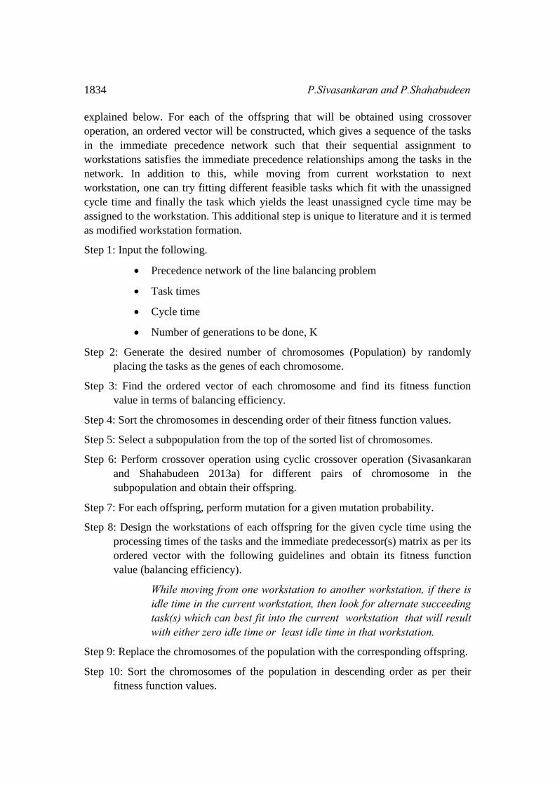
explained below. For each of the offspring that will be obtained using crossover

operation, an ordered vector will be constructed, which gives a sequence of the tasks

in the immediate precedence network such that their sequential assignment to

workstations satisfies the immediate precedence relationships among the tasks in the

network. In addition to this, while moving from current workstation to next

workstation, one can try fitting different feasible tasks which fit with the unassigned

cycle time and finally the task which yields the least unassigned cycle time may be

assigned to the workstation. This additional step is unique to literature and it is termed

as modified workstation formation.

Step 1: Input the following.

Precedence network of the line balancing problem

Task times

Cycle time

Number of generations to be done, K

Step 2: Generate the desired number of chromosomes (Population) by randomly

placing the tasks as the genes of each chromosome.

Step 3: Find the ordered vector of each chromosome and find its fitness function

value in terms of balancing efficiency.

Step 4: Sort the chromosomes in descending order of their fitness function values.

Step 5: Select a subpopulation from the top of the sorted list of chromosomes.

Step 6: Perform crossover operation using cyclic crossover operation (Sivasankaran

and Shahabudeen 2013a) for different pairs of chromosome in the

subpopulation and obtain their offspring.

Step 7: For each offspring, perform mutation for a given mutation probability.

Step 8: Design the workstations of each offspring for the given cycle time using the

processing times of the tasks and the immediate predecessor(s) matrix as per its

ordered vector with the following guidelines and obtain its fitness function

value (balancing efficiency).

While moving from one workstation to another workstation, if there is idle time in the current workstation, then look for alternate succeeding task(s) which can best fit into the current workstation that will result with either zero idle time or least idle time in that workstation.

Step 9: Replace the chromosomes of the population with the corresponding offspring.

Step 10: Sort the chromosomes of the population in descending order as per their

fitness function values.


Step 11: Increment the generation count k by 1.

Step 12: If the generation count k is less than or equal to K, then go to Step 5;

otherwise, go to Step 13.

Step13: Print the chromosome at the top of the sorted population as the final solution

along with its balancing efficiency.

Step 14: Stop

3.2 Genetic Algorithm to Solve Mixed-Model Assembly Line Balancing Problem

The steps of the genetic algorithm with cyclic crossover method and modified

workstation formation to solve mixed-model assembly line balancing problem are

explained below. As explained in the previous subsection, for each of the offspring

that will be obtained using crossover operation, an ordered vector will be constructed,

which gives a sequence of the tasks in the immediate precedence network such that

their sequential assignment to workstations satisfies the immediate precedence

relationships among the tasks in the network. In addition to this, while moving from

current workstation to next workstation, one can try fitting different feasible tasks

which fit with the unassigned cycle time and finally the task which yields the least

unassigned cycle time may be assigned to the current workstation.

Step 1: Input the following.

Number of models

Precedence networks of the models of the line balancing problem

Combined precedence network

Task times of the models

Cycle time of each model and average cycle time

Number of generations to be done, K

Step 2: Generate the desired number of chromosomes (Population) by randomly

placing the tasks as the genes of each chromosome.

Step 3: Find the ordered vector of each chromosome in the population.

Step 4: Assign the tasks to stations based on the combined precedence network and

with the original task times of the models.

Step 5: Find the fitness function value in terms of average balancing efficiency of the

models.

Step 6: Sort the chromosomes in descending order of their fitness function values.


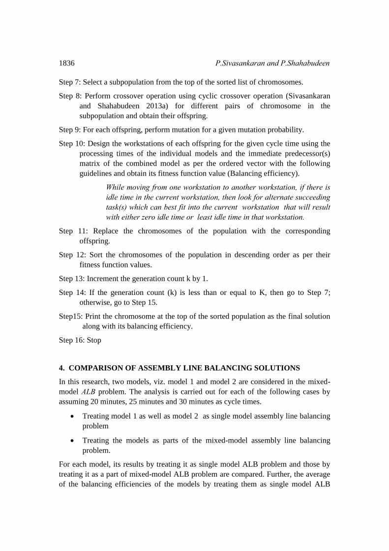
Step 7: Select a subpopulation from the top of the sorted list of chromosomes.

Step 8: Perform crossover operation using cyclic crossover operation (Sivasankaran

and Shahabudeen 2013a) for different pairs of chromosome in the

subpopulation and obtain their offspring.

Step 9: For each offspring, perform mutation for a given mutation probability.

Step 10: Design the workstations of each offspring for the given cycle time using the

processing times of the individual models and the immediate predecessor(s)

matrix of the combined model as per the ordered vector with the following

guidelines and obtain its fitness function value (Balancing efficiency).

While moving from one workstation to another workstation, if there is idle time in the current workstation, then look for alternate succeeding task(s) which can best fit into the current workstation that will result with either zero idle time or least idle time in that workstation.

Step 11: Replace the chromosomes of the population with the corresponding

offspring.

Step 12: Sort the chromosomes of the population in descending order as per their

fitness function values.

Step 13: Increment the generation count k by 1.

Step 14: If the generation count (k) is less than or equal to K, then go to Step 7;

otherwise, go to Step 15.

Step15: Print the chromosome at the top of the sorted population as the final solution

along with its balancing efficiency.

Step 16: Stop

4. COMPARISON OF ASSEMBLY LINE BALANCING SOLUTIONS

In this research, two models, viz. model 1 and model 2 are considered in the mixed-

model ALB problem. The analysis is carried out for each of the following cases by

assuming 20 minutes, 25 minutes and 30 minutes as cycle times.

Treating model 1 as well as model 2 as single model assembly line balancing

problem

Treating the models as parts of the mixed-model assembly line balancing

problem.

For each model, its results by treating it as single model ALB problem and those by

treating it as a part of mixed-model ALB problem are compared. Further, the average

of the balancing efficiencies of the models by treating them as single model ALB


problems and the average of the balancing efficiencies of the models by treating them

as parts of mixed-model ALB problem are also compared.

The analysis of the results of each of these cases is carried out using a complete

factorial experiment with three factors as listed below.

Problem Size (Factor A), which is represented by the number of nodes in the

network. The levels of this factor are 15 nodes, 20 nodes, 25 nodes, 30 nodes,

35 nodes and 40 nodes.

Assembly line balancing problem type (Factor B), whose levels are Single

model and Mixed- model. This is represented by ALB type.

Cycle time (Factor C), whose levels are 20 minutes, 25 minutes and 30

minutes.

Under each experimental combination, two replications are carried out. The model of

this ANOVA is as given below.

Yijkl = μ + Ai + Bj + ABij + Ck + ACik + BCjk + ABCijk + eijkl

where,

μ is the overall mean

Yijkl is the balancing efficiency of the lth replication under the ith level of the

factor A, jth level of the factor B and the kth level of the factor C.

Ai is the effect of the ith level of the factor A on the balancing efficiency

Bj is the effect of the jth level of the factor B on the balancing efficiency

ABij is the effect of the ith level of the factor A and the jth level of the factor B

on the balancing efficiency

Ck is the effect of the kth level of the factor C on the balancing efficiency

ACik is the effect of the ith level of the factor A and the kth level of the factor C


BCjk is the effect of the jth level of the factor B and the kth level of the factor C


ABCijk is the effect of the ith level of the factor A, jth level of the factor B and

the kth level of the factor C on the balancing efficiency

eijkl is the error associated with the balancing efficiency of the lth replication

under the ith level of the factor A, jth level of the factor B and the kth

level of the factor C.


4.1 Comparison of Balancing Efficiencies of Model 1

As per the complete factorial experiment presented earlier, the results of the balancing

efficiencies of the model 1 by treating it as a single model assembly line balancing

problem and as a part of the mixed model assembly line balancing problem are shown

in Table 1.

For the model 1, the balancing efficiencies of the six problems each with two

replications (totally 12 problems) using the single model approach and the mixed-

model approach for the cycle times of 20 minutes, 25 minutes and 30 minutes are

shown in the form of bar chart in Fig.4, Fig.5 and Fig.6, respectively. The problems

are numbered from 1 to 12. From Fig.4, one can verify that the balancing efficiency

obtained using the single model approach and that obtained using the mixed-model

approach are the same for the problem 1 (first replication of the problem with 15

nodes). Further, it is clear that for each of all other problems, the balancing efficiency

obtained using the single model approach is more than that obtained using the mixed

model approach, except for the problem 5 (first replication of the problem with 25

nodes). In Fig.5, for all the problems, the balancing efficiencies obtained using the

single model approach are more than the respective balancing efficiencies obtained

using the mixed model approach. In Fig.6, the balancing efficiencies obtained using

the single model approach and those obtained using the mixed-model approach are

the same for the problem 1 (first replication of the problem with 15 nodes) and the

problem 12 (second replication of the problem with 40 nodes). For all other problems,

the balancing efficiencies obtained using the single model approach are greater than

the respective balancing efficiencies obtained using the mixed model approach.

Based on these facts, one can conclude that for any problem, the balancing efficiency

obtained using the single model approach will be greater than the balancing efficiency

obtained using the mixed model approach. Now, the question is whether the

difference between them is statistically significant. This can be answered using a

carefully designed ANOVA experiment, which is already explained.

Table 1. Results of Balancing Efficiencies of Model 1

Problem size Replication ALB Type

Single Model Mixed-model

Cycle Time Cycle Time

20 min 25 min 30 min 20 min 25 min 30 min

15 1 80.83 97.00 80.83 80.83 77.6 80.83

2 82.50 99.00 82.50 70.71 66.00 66.00

20 1 91.25 83.43 97.33 73.00 64.89 69.52

2 92.50 84.57 98.67 74.00 65.78 70.40


25 1 88.00 88.00 97.78 97.78 78.22 83.81

2 83.50 95.43 92.78 69.58 83.50 79.52

30 1 88.33 94.22 88.33 75.71 77.09 78.52

2 82.92 88.44 94.76 58.53 66.33 73.70

35 1 92.27 90.22 84.58 72.50 73.82 75.19

2 88.75 94.67 88.75 81.92 85.20 88.75

40 1 86.92 90.40 94.17 66.47 75.33 75.33

2 92.69 87.64 89.26 86.07 80.33 89.25

Series 1 Balancing efficiencies of Model 1 using single model approach Series 2: Balancing efficiencies of Model 1 using mixed-model approach

Fig.4 Balancing efficiencies of Model 1 when cycle time is 20 minutes

Series 1 Balancing efficiencies of Model 1 using single model approach

Series 2: Balancing efficiencies of Model 1 using mixed-model approach Fig.5 Balancing efficiencies of Model 1 when cycle time is 25 minutes




For the data shown in Table 1, the results of ANOVA are shown in Table 2. From this

table, it is clear that the effect of the factor B “ALB type” on the balancing efficiency

is significant and the effects of all other components on the balancing efficiency are

insignificant at a significance level of 0.05. Since, the number of levels for ALB type

is only 2, the best “ALB type” in terms of balancing efficiency can be obtained by

comparing their mean balancing efficiencies. The mean balancing efficiency through

the single model assembly line balancing is 89.81% and that through the mixed-model

assembly line balancing is 75.89%. From this comparison, it is evident that the model

1 when it is solved by treating it as a single model gives better balancing efficiency.

Table 2. ANOVA Results of Balancing Efficiency of Model 1

Source of

Variation

Sum of

Squares

Degrees of

Freedom

Mean Sum

of Squares

F Ratio

(calculated)

Table F

value at

α=0.05

Remark

Problem Size

(A)

437.38 5 87.48 2.049 2.48 Insignificant

ALB Type (B) 3487.88 1 3487.88 81.703 4.12 Significant

AB 363.34 5 72.69 1.703 2.48 Insignificant

Cycle Time

(C)

82.94 2 41.47 0.971 3.27 Insignificant

AC 439.41 10 43.94 1.029 2.11 Insignificant

BC 68.69 2 34.34 0.804 3.27 Insignificant

ABC 376.88 10 37.60 0.881 2.11 Insignificant

Error 1536.75 36 42.69

Total 6792.27 71


4.2 Comparison of Balancing Efficiencies of Model 2

As per the complete factorial experiment presented earlier, the results of the balancing

efficiencies of the model 2 by treating it as a single model assembly line balancing

problem and as a part of the mixed model assembly line balancing problem are shown

in Table 3.

For the model 2, the balancing efficiencies of the 12 problems using the single model

approach and the mixed-model approach for the cycle times of 20 minutes, 25

minutes and 30 minutes are shown in the form of bar chart in Fig.7, Fig.8 and Fig.9,

respectively. From Fig.7, one can verify that the balancing efficiencies obtained using

the single model approach and those obtained using the mixed-model approach are

the same for the problem 2 (second replication of the problem with 15 nodes) and the

problem 5 (first replication of the problem with 25 nodes). Further, it is clear that for

each of all other problems, the balancing efficiency obtained using the single model

approach is more than that obtained using the mixed model approach. In Fig.8, for all

the problems, the balancing efficiencies obtained using the single model approach, are

more than the respective balancing efficiencies obtained using the mixed model

approach. In Fig.9, the balancing efficiencies obtained using the single model

approach and those obtained using the mixed-model approach are the same for the

problems 1 and 2, which are the first and the second replications of the problem with

15 nodes. For all other problems, the balancing efficiencies obtained using the single

model approach, are greater than the respective balancing efficiencies obtained using

the mixed model approach.

Based on these facts, one can conclude that for any problem, the balancing efficiency

obtained using the single model approach will be greater than the balancing efficiency

obtained using the mixed model approach. Now, the question is whether the

difference between them is statistically significant. As stated earlier, this can be

answered using a carefully designed ANOVA experiment, which is already explained.

For the data shown in Table 3, the results of ANOVA are shown in Table 4. From this

table, it is clear that the components of ANOVA, viz. Problem Size (A) and ALB

type (AB) are significant and all other components are insignificant at a significance

level of 0.05. Since, the number of levels of “ALB type” is only 2, the best ALB type

in terms of balancing efficiency can be obtained by comparing their mean balancing

efficiencies. The mean balancing efficiency using the single model approach is

89.72% and that using the mixed-model approach is 75.25%. From this comparison, it

is evident that the model 2 when it is solved by treating it as a single model gives

better balancing efficiency.


Table 3. Results of Balancing Efficiencies of Model 2





15 1 93.00 93.00 77.50 77.50 77.40 77.50

2 82.86 92.80 77.33 82.86 77.33 77.33

20 1 95.63 87.43 85.00 76.50 68.00 72.86

2 95.63 87.43 85.00 73.00 64.89 69.52

25 1 92.22 83.00 92.22 92.22 73.78 79.05

2 84.50 96.57 93.89 70.42 84.50 80.48

30 1 87.73 85.78 91.91 68.93 70.18 71.48

2 81.79 91.60 95.42 67.35 76.33 84.82

35 1 88.46 92.00 95.83 82.14 83.64 85.19

2 89.00 89.00 98.89 68.46 71.20 74.17

40 1 88.08 91.60 95.42 67.32 76.33 76.33

2 90.00 88.00 94.26 70.77 66.00 73.33




Table 4 ANOVA Results of Balancing Efficiency of Model 2

Source of

Variation

Sum of

Squares

Degrees

of

Freedom

Mean Sum

of Squares

F Ratio

(calculated)

Table F

value at

α=0.05

Remark

Problem Size

(A)

263.00 5 52.60 1.962 2.48 Insignificant


AB 319.91 5 63.98 2.386 2.48 Insignificant

Cycle Time

(C)

39.31 2 19.66 0.733 3.27 Insignificant

AC 609.53 10 60.95 2.273 2.11 Significant



Error 965.22 36 26.81

Total 6151.16 71

4.3 Comparison of Average Balancing Efficiencies of Model 1 and Model 2

As per the complete factorial experiment presented earlier, the results of the average

balancing efficiencies of the model 1 and model 2 by treating them as single model

assembly line balancing problem and mixed model assembly line balancing problem

are shown in Table 5.

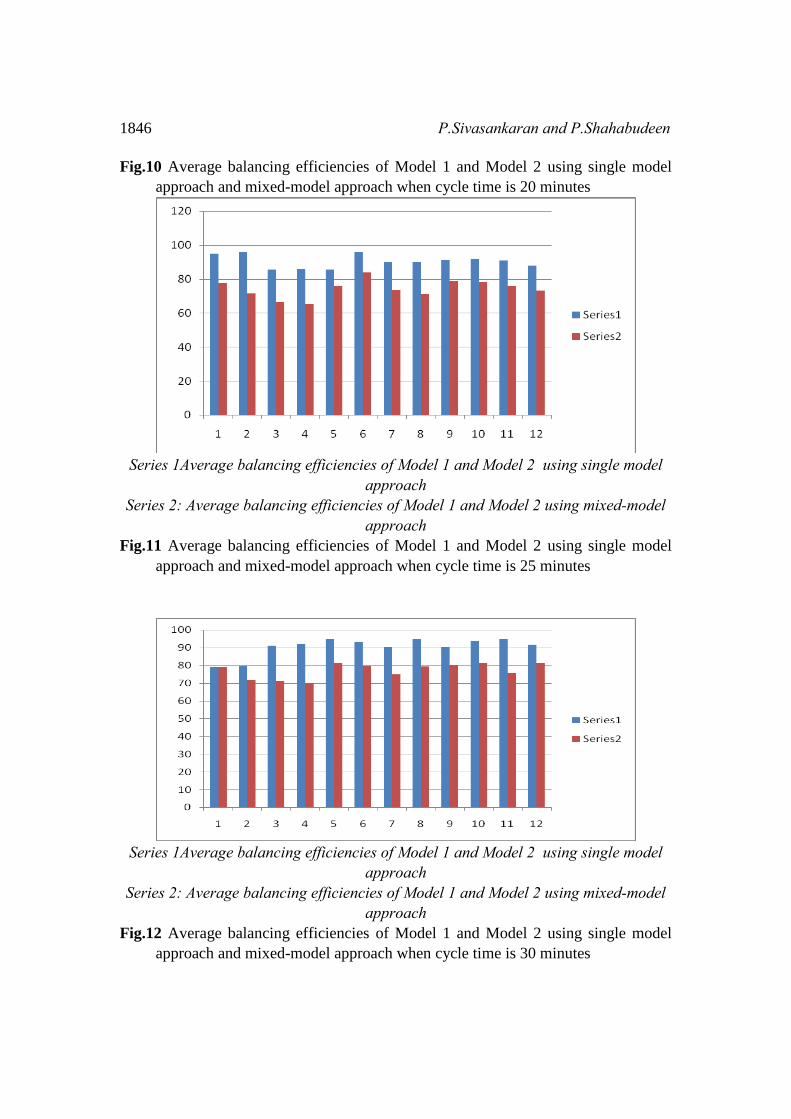
The averages of the balancing efficiencies of model 1 and model 2 of the 12 problems

using the single model approach and the mixed-model approach for the cycle times of

20 minutes, 25 minutes and 30 minutes are shown in the form of bar chart in Fig.10,

Fig.11 and Fig.12, respectively. From Fig.10 and Fig.11, one can verify that for each

problem, the average of the balancing efficiencies of the model 1 and the model 2

obtained using the single model approach is greater than that obtained using the

mixed-model approach. In Fig.12, the same holds good except for the problem 1 (first

replication of the problem with 15 nodes) for which they are same.

Based on these facts, it is found that for any problem, the average of the balancing

efficiencies of the models 1 and 2 obtained using the single model approach will be

greater that the average of the balancing efficiencies of the models 1 and 2 obtained

using the mixed model approach. Now, the question is whether the difference

between them is statistically significant. This can be answered using a carefully

designed ANOVA experiment, which is already explained.

The results of ANOVA of the data shown in Table 5 are presented in Table 6. From

this table, it is clear that the components of ANOVA, viz. Problem Size (A), ALB

type (B), the interaction terms of AB and AC are significant and all other components

are insignificant at a significance level of 0.05. Since, the number of levels of factor


B (ALB type) is only two, the best ALB type in terms of average balancing efficiency

can be obtained by comparing their mean of the average balancing efficiencies. The

mean of the average balancing efficiencies of the model 1 and the model 2 obtained

using the single model approach is 89.77% and that obtained using mixed-model

approach is 75.57%. From this comparison, it is evident that the best average

balancing efficiency is obtained when the models 1 and 2 are solved by treating them

as single model ALB problems.

Table 5 Results of Average Balancing Efficiencies of Model 1 and Model 2





15 1 86.92 95.00 79.17 79.17 77.50 79.17

2 82.68 95.90 79.92 76.79 71.67 71.67

20 1 93.44 85.43 91.17 74.75 66.45 71.19

2 94.07 86.00 91.84 73.5 65.34 69.96

25 1 90.11 85.50 95.00 95.00 76.00 81.43

2 84.00 96.00 93.34 70.00 84.00 80.00

30 1 88.03 90.00 90.12 72.32 73.64 75.00

2 82.36 90.02 95.09 62.94 71.33 79.26

35 1 90.37 91.11 90.21 77.32 78.73 80.19

2 88.88 91.84 93.82 75.19 78.20 81.46

40 1 87.50 91.00 94.80 66.90 75.83 75.83

2 91.35 87.82 91.76 78.42 73.17 81.29

Series 1Average balancing efficiencies of Model 1 and Model 2 using single model

approach Series 2: Average balancing efficiencies of Model 1 and Model 2 using mixed-model

approach


Fig.10 Average balancing efficiencies of Model 1 and Model 2 using single model

approach and mixed-model approach when cycle time is 20 minutes



approach Fig.11 Average balancing efficiencies of Model 1 and Model 2 using single model




approach Fig.12 Average balancing efficiencies of Model 1 and Model 2 using single model



Table 6 ANOVA Results of Average Balancing Efficiency of Models

Source of

Variation

Sum of

Squares

Degrees

of

Freedom

Mean

Sum of

Squares

F Ratio

(calculated)

Table F

value at

α=0.05

Remark

Problem Size

(A)

309.38 5 61.876 3.284 2.48 Significant


AB 242.25 5 48.45 2.572 2.48 Significant

Cycle Time

(C)

56.22 2 28.11 1.492 3.27 Insignificant

AC 431.41 10 43.141 2.290 2.11 Significant



Error 678.25 36 18.84

Total 5555.89 71

The results of all the three subsections of this section indicate that it is better to solve

each model by treating it as a single model to have the best solution in terms of

balancing efficiency.

5. CONCLUSION

Assembly line balancing problem is an important issue in all mass production systems

to improve their productivity as well as to meet customer demand. The mixed-model

assembly line balancing problem gains importance because of the increased focus of

batch manufacturing in mass production, which produces more than one product

simultaneously in the same line.

If one examines the balancing efficiencies of the models that are assembled using the

mixed-model approach with those of the models that are assembled using the single

model approach, there will be differences.

In this paper, an attempt has been made to compare the balancing loss of the mixed-

model assembly line balancing for a given set of models in comparison with that of

the single model assembly line balancing. The analysis is done with respect to the

balancing efficiency of each model and the average balancing efficiency of the

models.

In each analysis, it is found that for most of the cases, the results using the single

model approach are better than the corresponding results using the mixed model

approach. But, to prove statistically, it is highly essential to conduct a design of


experiment for this situation. So, a complete factorial experiment has been carried out

in which three factors, viz. Problem Size (A), ALB Type (B) and Cycle Time (C) are

considered, with two replications under each experimental combination. The number

of models in the mixed-model is 2. In each of the three analyses, it is found that there

is significant difference between the treatments of the factor “ALB type” (B). The

mean balancing efficiency obtained using the single model approach is better than

that obtained using the mixed-model approach.

Based on this analysis, practitioners are recommended to use the mixed-model

assembly line balancing approach if there is a necessity to supply the models with

small volume on daily basis. If the volume of each model is above medium level to

justify a separate assembly line, then the company can setup a separate line for each

model to take advantage of the best balancing efficiency.

REFERENCE

[1] Deckro, R.F. and Rangachari, S., 1990, A goal approach to assembly line

balancing, Computers and Operations Research, 17, 509–521.

[2] Fattahi, P. and Salehi, M., 2009, Sequencing the mixed-model assembly line

to minimize the total utility and idle costs with variable launching interval.

International Journal of Advanced Manufacturing Technology, 45, 987–998.

[3] Genikomsakis, K.N. and Tourassis, V.D., 2012, Task proximity index: a novel

measure for assessing the work-efficiency of assembly line balancing

configurations, International Journal of Production Research, 50,1624-1638.

[4] Gokcen, H. and Erel, E., 1997, A goal programming approach to mixed model

assembly line balancing problem, International Journal of Production

Economics, 48, 177-185.

[5] Gokcen, H. and Erel, E., 1998, Binary integer formulation for mixed-model

assembly line balancing problem, Computers & Industrial Engineering, 34(2),

451-461.

[6] Hong, D.S. and Cho, H.S., 1997, Generation of robotic assembly sequences

with consideration of line balancing using simulated annealing, Robotica, 15,

663–674.

[7] Hop, N.V., 2006, A heuristics solution for fuzzy mixed-modelling balancing

problem, European Journal of Operational Research, 168, 798-810.

[8] J. Rubinnovitz and G. Levitin, 1995, Genetic algorithm for assembly line

balancing, International Journal of Production Economics, 41, 343-354.

[9] Jin, M. and Wu, S.D., 2002, A new heuristic method for mixed-model

assembly line balancing problem, Computers & Industrial Engineering, 44,

159-169.

[10] Kara, Y., Ozgiiven, C., Seeme, N.Y. and Ching-Ter Chang, 2011, Multi-


objective approaches to balance mixed-model assembly lines for model mixes

having precedence conflicts and duplicate common tasks, International

Journal of Advanced Manufacturing Technology, 52, 725-737.

[11] Kilincci, O., 2011, Firing sequences backward algorithm for simple assembly

line balancing problem of type 1, Computers and Industrial Engineering,

60(4), 830-839.

[12] Kim, Y.K. and Kim, J.Y., 2000, A co-evolutionary algorithm for balancing

and sequencing in mixed-model assembly lines, Applied Intelligence, 13,

247-258.

[13] Matanachai. S. and Yano, C.A., 2001, Balancing mixed-model assembly lines

to reduce work overload, IIE Transactions, 33, 29-42.

[14] Mutlu, O. and Ozgormus, E., 2012, A fuzzy assembly line balancing problem

with physical workload constraints, International Journal of Production

Research, 50, 5281-5291.

[15] Narayanan, S. and Panneerselvam, R., 2000, New efficient set of heuristics for

assembly line balancing, International Journal of Management and Systems,

16, 287–300.

[16] Ozcan, U., Cercioglu, H., Gokcen, H. and Toklu, B., 2010, Balancing and

sequencing of parallel mixed-model assembly lines. International Journal of

Production Research, 48(17), 5089–5113

[17] Panneerselvam, R. and Sankar, C.O., 1993, New heuristics for assembly line

balancing problem, International Journal of Management and Systems, 9, 25–

36.

[18] Pastor, R., 2011, LB-ALBP: the lexicographic bottleneck assembly line

balancing problem, International Journal of Production Research, 9, 2425-

2442.

[19] Ponnambalam, S.G., Aravindan, P. and Naidu, G.M., 2000, A multi-objective

genetic algorithm for solving assembly line balancing problem, International

Journal of Advanced Manufacturing Technology, 16, 341–352.

[20] Sabuncuoglu, I., Erel, E. and Tanyer, M., 2000, Assembly line balancing using

genetic algorithm, Journal of Intelligent Manufacturing, 11, 295-310.

[21] Sivasankaran, P. and Shahabudeen, P., 2013a, Genetic Algorithm for

Concurrent Balancing of Mixed-Model Assembly Lines with Original Task

Times of Models, Intelligent Information Management, 5, 84-92.

[22] Sivasankaran, P. and Shahabudeen, P., 2013b, Modelling hybrid single model

assembly line balancing problem, UDYOG PRAGATI, 37(1), 26-36.

[23] Sivasankaran, P., Shahabudeen, P., Analysis of single model and mixed-model

assembly line balancing solutions, International Conference on Advances in

Industrial Engineering Applications 2014 (ICAIEA2014), 6-8 January, 2014,

Anna University, Chennai, India.


[24] Thangavelu, S.R. and Shetty, C.M., 1971, Assembly line balancing by zero-

one integer programming, IIE Transactions, 3, 61–68.

[25] Zhang, X.M. and Han, X.C., 2012, The balance problem solving of the car

mixed-model assembly line based on hybrid differential evolution algorithm,

Applied Mechanics and Materials, 220-223, 178-183.

Comparison of Single Model and Multi-Model Assembly Line ... · assembly line balancing problems in...

Documents

Transcript of Comparison of Single Model and Multi-Model Assembly Line ... · assembly line balancing problems in...