Comparison of Results in Flexible Multibody Dynamics Using Various...
25
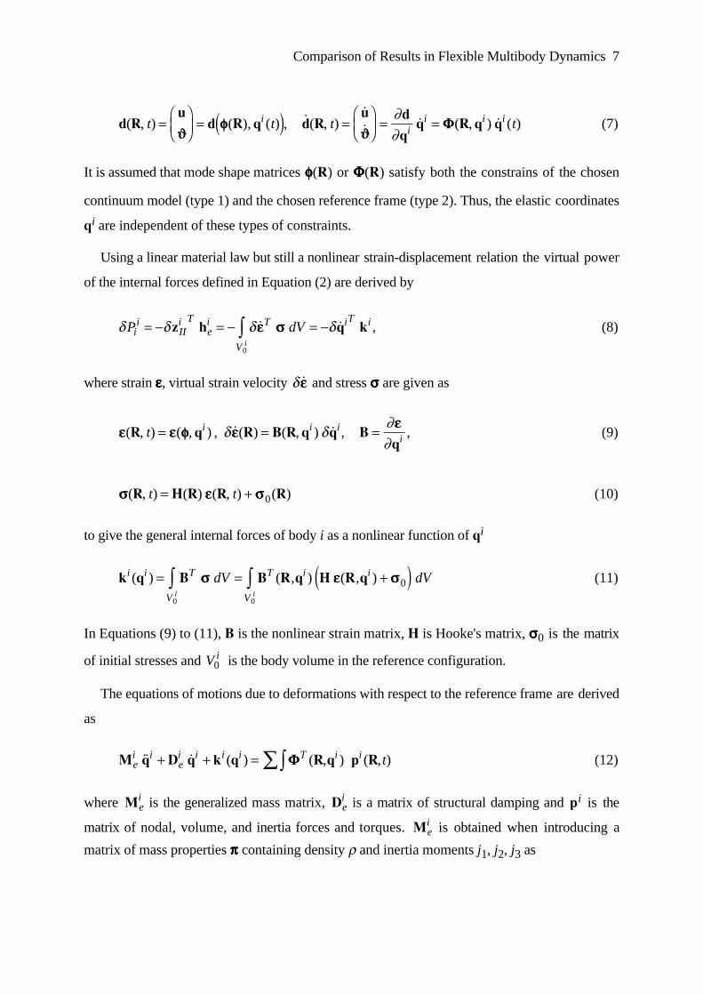
Nonlinear Dynamics Comparison of Results in Flexible Multibody Dynamics Using Various Approaches OSKAR WALLRAPP Department of Precision and Micro Engineering, Munich University of Applied Sciences, Lothstr. 34, D-80335 Munich, Germany, e-mail: [email protected] SIMON WIEDEMANN Lenaustrasse 2, D-81373 Munich, Germany, e-mail: simon.wiedemann@web Abstract. Throughout the past decades a considerable amount of work has been dedicated to the development and application of formalisms to simulate flexible bodies in a multibody system (MBS). The two most common approaches to describe the deformation of a flexible body with respect to their floating frame of reference are to apply the linear finite element formulation and the linear modal approach using global mode shapes. On the field of flexible body modelling, this paper discusses two topics: a) the consideration of quadratic terms in the equations of deformation and b) the presentation of methods for global mode preparation to reduce the computer time for dynamic simulations without loss of accuracy regarding deformations. The proposed methods are applied in two examples, for the deformation of a stabilisation linkage of a car's front suspension and for the simulation of the deployment of a flexible solar array. Keywords: Multibody simulation, flexible body modelling, nodal and modal coordinates, mode selection 1. Introduction For the simulation and analysis of flexible mechanical systems, the multibody system (MBS) theory is applied. In this methodology, a flexible multibody systems is based on the floating frame of reference formulation with superimposed deformations. Then the flexible body motion is the sum of a large reference motion and small deformations. The displacement field due to deformation is approximated by summing the products of known shape functions and unknown weighing coefficients. The shape functions may be obtained using the finite element approach, where local polynomial functions represent the nodal coordinates or the modal approach, where
Transcript of Comparison of Results in Flexible Multibody Dynamics Using Various...
Nonlinear Dynamics
Comparison of Results in Flexible MultibodyDynamics Using Various Approaches
OSKAR WALLRAPP
Department of Precision and Micro Engineering, Munich University of Applied Sciences, Lothstr. 34, D-80335
Munich, Germany, e-mail: [email protected]
SIMON WIEDEMANN
Lenaustrasse 2, D-81373 Munich, Germany, e-mail: simon.wiedemann@web
Abstract. Throughout the past decades a considerable amount of work has been dedicated to the development
and application of formalisms to simulate flexible bodies in a multibody system (MBS). The two most common
approaches to describe the deformation of a flexible body with respect to their floating frame of reference are to
apply the linear finite element formulation and the linear modal approach using global mode shapes.
On the field of flexible body modelling, this paper discusses two topics: a) the consideration of quadratic
terms in the equations of deformation and b) the presentation of methods for global mode preparation to reduce
the computer time for dynamic simulations without loss of accuracy regarding deformations.
The proposed methods are applied in two examples, for the deformation of a stabilisation linkage of a car's
front suspension and for the simulation of the deployment of a flexible solar array.
Keywords: Multibody simulation, flexible body modelling, nodal and modal coordinates, mode selection
1. Introduction
For the simulation and analysis of flexible mechanical systems, the multibody system (MBS)
theory is applied. In this methodology, a flexible multibody systems is based on the floating
frame of reference formulation with superimposed deformations. Then the flexible body motion
is the sum of a large reference motion and small deformations. The displacement field due to
deformation is approximated by summing the products of known shape functions and unknown
weighing coefficients. The shape functions may be obtained using the finite element approach,
where local polynomial functions represent the nodal coordinates or the modal approach, where

2 O. Wallrapp and S. Wiedemann
global eigenfunctions or static displacement fields represent modal amplitudes. The latter
approach reduces the system order but gives rise to the problem of selecting the shape
functions. In the following we assume that the strain and displacements are small, but
shortening and tilting effects due to high loads should be considered during calculation of the
displacement field. The material law is linear.
The multibody system software SIMPACK [4] is based on the formulation above, and the
data of flexible bodies are taken from the SID file, and prepared in pre-processors SIMBEAM
[10] for spatial beam structures and in FEMBS for general spatial finite element structures in
connection with all important commercial finite element software like ANSYS, NASTRAN,
etc. The pre-processors generate all mass and stiffness data needed in SIMPACK including
geometric stiffness matrices. These prove to be important when buckling or stiffening effects
due to large longitudinal loads have to be taken into account [11].
As shown in [10], [3] the linear theory of elasticity is often not accurate enough when
structures experience loads that approach the critical loads for buckling and tilting or when
spatial bending effects are considered. In such cases a non-linear beam theory or a substructure
technique is more suitable. In this paper, kinematic displacement computations are made using
also the quadratic terms. The method is implemented in SIMPACK and all required matrices
can be pre-calculated in SIMBEAM.
The advantage of the modal approach is the small number of degrees of freedom, thus
reducing the computational burden considerably compared to the nodal approach. The modal
method however requires the pre-calculation of the mode shapes to be used (for example by
solving eigen systems or static problems) in advance of the simulations. As many authors have
shown, the quality of results obtained with the modal approach depends (besides numerical
aspects) exclusively on the quality of the mode shapes used in the simulations, that is on how
accurate the mode shapes can represent the real deformations. Thus since the actual loads, load
frequencies and deformations of the bodies are usually not known beforehand, the choice of
mode shapes is often random (assumed modes), as are the results of such simulations. It is
known that even a very small number of proper mode shapes can lead to results close to or
equal to those obtained with a FE approach.
This paper discusses methods for a proper selection of mode shapes in advance of the
simulations and compares results using both the nodal and modal approach. Additionally, the

Comparison of Results in Flexible Multibody Dynamics 3
influence of the geometric stiffness matrices and kinematic displacement computation with
quadratic terms is studied. The results are compared with results obtained using ANSYS and
the nonlinear absolute nodal coordinate formulation (ANCF) [2].
The first example of a stabilisation linkage of a car's front suspension (Figure 1) is a spatial
beam structure that is modelled using SIMBEAM. Static and dynamical load cases are simulated
using SIMBEAM and SIMPACK. The second example is a flexible satellite solar array (Figure
2). The goal of the simulation is to compute the flexible behaviour during deployment. In
addition to [12] new methods for mode shape creation are applied to increase accuracy and to
reduce the computational burden. The mode shapes of the flexible bodies (yoke and six panels)
are created using NASTRAN and FEMBS and the deployment simulation is made using
SIMPACK.
Linkage
Figure 1. Stabilisation linkage of a car's front suspension.
Figure 2. Deployment of a flexible solar array.

4 O. Wallrapp and S. Wiedemann
2. Basics on Flexible Multibody System Theory
A brief description of the equations of motion of a flexible multibody system as published in
many papers [5, 7] is given to explain the notation and to give an overview of the assumptions
made for such formulations.
Consider a multibody system of n bodies where the motion is described by a set of position
and velocity variables zIi (t) and zII
i (t), respectively for each body i. A multibody system may
now be obtained from the general model of continuum mechanics by formulating three types of
constraint equations: (1) definition of the models of bodies (i.e. finite element models, beams,
etc.) to be used for a specific analysis; (2) introducing a specific floating frame of reference to
describe body deformations; (3) constraints due to joints between the nodes on the bodies. The
explicit form of constraints of types 1 and 2 relates the displacement field of all the points of the
multibody system to the variables zIi and zII
i , where z Z zIi i
IIi= . Holonomic constraints of
type 3 due joints a = 1, .. nc, between bodies i and j can be written implicitly as
g z z 0 G z G zg
Gg
zZ G
g
zZa
Ii
Ij ai
IIi aj
IIj
aai
a
Ii
i aja
Ij
jtt
( , , ) ,= ¤ + + = = =∂∂
∂∂
∂∂
0 with . (1)
Formulating all types of constraint equations and applying one of the principles of dynamics,
one can generate the system equations in descriptor form or in state space form. An intermediate
result of such a derivation of the equations of motion for a system of n flexible bodies is the
virtual power expression due to inertia, internal forces of elasticity and applied body and
surface forces
d wP IIi T i
IIi i
ei
gi
fi
ci
i
n
= - + + + + +( ) ==
 ddz M z h h h h h˙ 01
. (2)
The matrices ddzIIi are the virtual velocities, belonging to the generalized velocities zII
i , Mi and
hci are the corresponding generalized masses and constraint forces, respectively. hw
i are
generalised inertia forces due to motion of the body reference frame, hei represents the internal
forces due to deformations, and hgi and h f
i consider gravitational forces and nodal forces and
torques on body i, respectively.

Comparison of Results in Flexible Multibody Dynamics 5
Jourdain's principle states that the virtual power of the constraint forces, result of all types of
constraints, is zero. In Equation (2), the virtual power expressions due to constraints of type 1
and 2 do not appear, but the virtual power due to constraints of type 3 is given explicitly. The
expression
M z h h h h hiIIi i
ei
gi
fi
ci˙ = + + + +w (3)
together with Equation (1) are the equations of motion of a body i, where hci are the generalised
constraint forces due to joints on body i.
In this formulation the flexible body motion is separated into a motion of a floating frame of
reference and small deformations. The displacement field due to deformation is approximated
by summing the products of known shape functions and unknown weighing coefficients, called
the elastic coordinates. Hence, the absolute position r of a point P at physical coordinate R on
body i at time t is given by the absolute position ri of the body reference frame { , }Oi ie with
respect to the inertia frame { , }OI Ie and the relative position r R( ) , see Figure 3. Here and in
all the following, vectors are expressed in coordinates of the body reference frame and are
indicated by a bold letter, but the time dependence of variables is not always written.
P
R
P
i
{O i, e i }
k
r k
R ku k
ur
node k on body ibody i
(reference configuration)
body i(actual configuration)
inertial coordinate system {O I, e I }
coordinate system {O k, e k }in actual configuration
coordinate system {O k, e k }in reference configuration
Figure 3 General model of a flexible body i.

6 O. Wallrapp and S. Wiedemann
The absolute position of P is expressed as
rr rr( ) ( ) ( ) ( )R r R r R R u R= + = +i where , (4)
and where u(R, t ) is the elastic deflection at R.
The absolute orientation of a coordinate system { , }P e attached to a section of a body (in
case of beam models attached to the beam section at R 1) or of a frame { , }Ok ke at a node k on
body i (Figure 3) is given by the product of the orientation matrix A i of the body reference
frame with respect to the inertia frame and the orientation matrix QQ( )R of the section frame with
respect to the body reference frame as
A R R A e A R e( ) ( ) ( )= =QQ i I satisfying (5)
Matrices Ai and QQQQ are parameterised by angles aai t( ) and JJ( , )R t , respectively.
Linear velocity v and angular velocities wwww of a body section at point P are derived by
differentiation of Equation (4) with respect to time and using the Poisson formula on Equation
(5), thus
v R v r R r R v r R r R
R w R
A A w w
r R u R w W
( ) ˜ ( ) ˙( ) ˜( ) ˙( )
( ) ( )
˜ ˜ ˙ , ˜ ˜ ˙ ,
˙( ) ˙ ( ) ˙
= + + = - +
= +
∫ = ∫ =
=
i i i i
i
i i iI i iT i ki T
ww ww
ww ww
ww ww QQ QQ
JJ JJ
satisfying
where and = ( )
(6)
Note that vi and wwi are the linear and angular velocities of the reference frame. Variables rri ,
A i , vi and wwi depend on time t and describe the motion of the reference frame of body i.
Variables r, QQQQ, r , and w or u, JJJJ, u, and JJ depend on coordinates R and time t and represent
the deformation of the body. Referring to the specific floating frames of reference such as
tangent frame, cord / plane frame, or Tisserand / Buckens frame, u and JJJJ have to satisfy six
constraints of reference conditions given in [7].
The deformation variables in Equations (4) to (6) are approximated by known shape
functions ffff(R) and time dependent weighing coefficients or elastic coordinates qi(t). In general
we can write
Comparison of Results in Flexible Multibody Dynamics 7
d Ru
d R q d Ru d
qq R q q( , ) ( ), ( ) , ˙ ( , )
˙˙ ˙ ( , ) ˙ ( )t t t ti
ii i i=
ÊËÁ
ˆ¯
= ( ) =ÊËÁ
ˆ¯
= =JJ
ffJJ
FF∂∂
(7)
It is assumed that mode shape matrices ffff(R) or FFFF(R) satisfy both the constrains of the chosen
continuum model (type 1) and the chosen reference frame (type 2). Thus, the elastic coordinates
qi are independent of these types of constraints.
Using a linear material law but still a nonlinear strain-displacement relation the virtual power
of the internal forces defined in Equation (2) are derived by
d d d dP dVii
IIi T
ei T
V
iT i
i
= - = - = -Úz h q k˙ ˙ee ss0
, (8)
where strain eeee, virtual strain velocity d ee and stress ssss are given as
ee ee ff eeee
( , ) ( , ) , ˙( ) ( , ) ˙R q R B R q q Bq
t i i ii= = =d d ∂
∂, , (9)
ss ee ss( , ) ( ) ( , ) ( )R H R R Rt t= + 0 (10)
to give the general internal forces of body i as a nonlinear function of qi
k q B B R q H R qi i T
V
T i i
V
dV dVi i
( ) ( , ) ( , )= = +( )Ú Úss ee ss0 0
0 (11)
In Equations (9) to (11), B is the nonlinear strain matrix, H is Hooke's matrix, ssss0 is the matrix
of initial stresses and V i0 is the body volume in the reference configuration.
The equations of motions due to deformations with respect to the reference frame are derived
as
M q D q k q R q p Rei i
ei i i i T i i t˙ ˙ ( ) ( , ) ( , )+ + = ÚÂ FF (12)
where Mei is the generalized mass matrix, De
i is a matrix of structural damping and pi is the
matrix of nodal, volume, and inertia forces and torques. Mei is obtained when introducing a
matrix of mass properties pppp containing density r and inertia moments j1, j2, j3 as
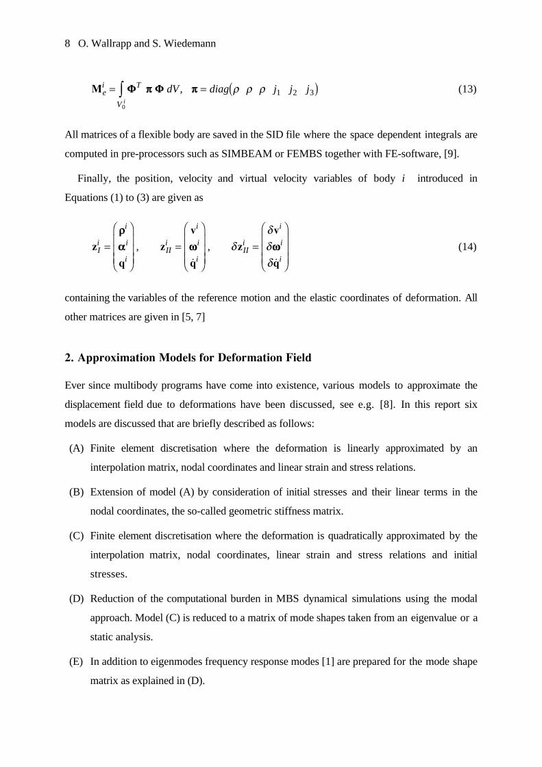
8 O. Wallrapp and S. Wiedemann
Mei T
V
dV diag j j ji
= = ( )Ú FF pp FF pp0
1 2 3, r r r (13)
All matrices of a flexible body are saved in the SID file where the space dependent integrals are
computed in pre-processors such as SIMBEAM or FEMBS together with FE-software, [9].
Finally, the position, velocity and virtual velocity variables of body i introduced in
Equations (1) to (3) are given as
z
q
z
v
q
z
v
qIi
i
i
iIIi
i
i
iIIi
i
i
i
=
Ê
Ë
ÁÁÁ
ˆ
¯
˜˜˜
=
Ê
Ë
ÁÁÁ
ˆ
¯
˜˜˜
=
Ê
Ë
ÁÁÁ
ˆ
¯
˜˜˜
rraa ww ww,
˙
,
˙
dddd
(14)
containing the variables of the reference motion and the elastic coordinates of deformation. All
other matrices are given in [5, 7]
2. Approximation Models for Deformation Field
Ever since multibody programs have come into existence, various models to approximate the
displacement field due to deformations have been discussed, see e.g. [8]. In this report six
models are discussed that are briefly described as follows:
(A) Finite element discretisation where the deformation is linearly approximated by an
interpolation matrix, nodal coordinates and linear strain and stress relations.
(B) Extension of model (A) by consideration of initial stresses and their linear terms in the
nodal coordinates, the so-called geometric stiffness matrix.
(C) Finite element discretisation where the deformation is quadratically approximated by the
interpolation matrix, nodal coordinates, linear strain and stress relations and initial
stresses.
(D) Reduction of the computational burden in MBS dynamical simulations using the modal
approach. Model (C) is reduced to a matrix of mode shapes taken from an eigenvalue or a
static analysis.
(E) In addition to eigenmodes frequency response modes [1] are prepared for the mode shape
matrix as explained in (D).
Comparison of Results in Flexible Multibody Dynamics 9
(F) The mode shapes taken from models (D) and (E) are selected using participation factors
[12].
For comparison of these models, results are partly taken from a nonlinear finite element
theory – here the absolute nodal coordinate formulation (ANCF) [2] and ANSYS. The six
models are described in detail next.
2 . 1 Model (A) – Linear FE Formulation
The simplest model is a linear expression of the deformation field in Equation (7). Thus, the
deformation field of an element e at all local element points x is described by the interpolation
matrix Ne(x) and nodal element coordinates ze(t). One finds the following relations for the
deformation, strain eeee and stress ssss of element e (denoted by the superscript e)
d R N x z d R N x ze e e e e et t t t( , ) ( ) ( ), ˙ ( , ) ( ) ˙ ( )= = and (15)
ee ee ss eeeLe e
Le e e e et t t t( , ) ( ) ( ) , ˙ ˙ , ( , ) ( ) ( , )x B x z B z x H x x= = =d d , (16)
where x R R= - e and Re is the position vector of the local element frame, BLe is the linear
strain and He the linear Hooke matrix of an element e.
The motion of all elements can be written by all global nodes forming the nodal coordinate
vector zF of the unsupported finite element (FE) structure. Finally, a nodal state vector yF of
the supported structure embedded into the MBS floating frame of reference is introduced,
satifsying both,
z T ze eF= and z J y J zF F F F F= + , (17)
where Te ist a transformation matrix and JF and JF are projection matrices for the free and
locked motions of the FE-boundaries. In Equation (17) the supported node motion zF is
mostly zero. This leads with the identy q yiF∫ and Equation (15) in accordance to (7)
d q R N x T J= ∫ =FF FF FFiL
e eF where ( ) ( ) . (18)
FFL is the linear mode shape matrix. From Equations (15) and (16) one derives the internal
forces and the mass matrix as given in Equations (11) to (13)

10 O. Wallrapp and S. Wiedemann
k q K q K J T K T J K B H Bi iei i
ei
FT eT e e
Fe
eLeT e
Le e
V
dVe
( ) ,= = ( ) =Â Ú ,
0
(19)
M J T M T J M N Nei
FT eT e e
Fe
e eT e e e
V
dVe
= ( ) =Â Ú , pp0
(20)
Ke and Me respectively are the element stiffness and mass matrices.
For various models of finite elements, interpolation matrices and their stiffness and mass
matrices are given in standard FE books. Model (A) is only useful for small elastic
deformations. The loads should be small compared to critical loads, for example for buckling
and tilting.
2 . 2 Model (B) – Geometric Stiffness Matrix
Model (A) is extended by initial stresses ssss0 as shown in Equation (10) and a bilinear term in the
virtual strain velocity, Equation (9). This bilinear term may be derived by a geometrically
nonlinear theory, for example for beam [5] and plate models. With the interpolation matrix
given for model (A), one finds instead of Equations (16) and (19)
ee ss ee sseLe e
Le eT
Qe e e e e
oe= = +( ) = +B z B z B z H, ˙ ˙ ,de da a a (21)
k q K K q K J T K T Ji iei i i i
FT eT e e
Fe
( ) = +( ) = ( )Âgeo geo geo, . (22)
In Equation (21) subscript a depends on the strain variables of a FE model. Matrix K geoi is the
geometric stiffness matrix. The element matrix K geoe leads to the specific initial element stresses
ssoe that are caused by initial loads on FE structures.
Applying the linear theory of elasticity, the actual geometric stiffness matrix of an element
can be expressed as a superposition of single load cases Lj on body i and unit geometric
stiffness matrices
)K geoj
e that are pre-calculated for unit loads. This gives unit stresses ssoje , see
e.g. [11],
K K K Bgeo geo geoe
je
je
jj
QeT
je e
V
L dVe
= =Â ÚÂ) )
, a aa
s 0
0
(23)

Comparison of Results in Flexible Multibody Dynamics 11
For the deformations and the mass matrix, Equations (18) and (20) are still applied.
Model (B) allows to calculate the critical buckling and tilting load for beam structures and to
take other stiffening effects into account, for example on rotating structures. On the other hand,
it should be noted that the model does not compute nonlinear displacements such as the
shortening of a beam when bent.
2 . 3 Model (C) – Quadratic Formulation of Deformations
Applying nonlinear theory, for example for a beam element, the Cartesian deformation variables
d contain quadratic terms and are expressed by integrals of the beam deformations such as
longitudinal strain e and the three curvatures ka. The strain relation (21) is still valid, but for d
= (da) instead of Equations (15) and (18) one writes with the linear shape function matrix
N NLe
Le= ( )a and a 6¥6 quadratic expansion shape function matrix NQ
ea , for direction a,
d
d
Le e eT
Qe e
Li iT
Qi
a a a
a a a a
( ) ( ) ( )
( ) ( ) ( ) , ,...
x N x z z N x z
R R q q R q
= +
= + =
12
12 1 6
and
FF FF(24)
Note that FFQa is a nq ¥nq matrix given as
FFQT eT
Qe e
ea a( ) ( )R T T N x T T= ( )Â . (25)
If the longitudinal stress and the bending moment of a beam element is constant with respect to
the central axis x, then matrices NQe
a at node k are equivalent to the negative values of the unit
geometric stiffness matrices
)K geo j
e , where j denotes the load case at node k in direction a .
More details are given in [10].
Model (C) gives better results than models (A) and (B) if the actual loads approach the
critical loads for buckling or tilting or if three dimensional bending and torsion motions of beam
elements are analysed.
2 . 4 Model (D) – Modal Transformation
The modal approximation is applied. The deformation of the FE structure of a body i is given
by Equation (12) where damping is neglected and internal forces are incorporated by a simple
stiffness matrix as given in Equation (19). This leads the equations of motion of a FE-structure
12 O. Wallrapp and S. Wiedemann
M y K y pei
F ei
F LT i˙ + = ÚÂ FF , (26)
where yF is the vector of nodal coordinates of the supported FE structure. The length nyF of
yF is in general very large.
With Equation (26) eigenvectors and static displacement fields due to specific load cases
(static modes) can be created to give a small number (nq ) of mode shapes that are taken into ac-
count in the dynamic MBS simulation. The selected mode shapes form the mode matrix Se with
dimensions nyF times nq. This yields the new mass, stiffness (modal) and mode shape matrices
as
y S q
M S M S K S K S S
F ei
ei
eT
ei
e ei
eT
ei
e e
=
= = =
and
: , : , :FF FF(27)
respectively, with the reduced dimension nq to approximately describe the deformation of the
flexible body as shown in Equation (12). It should be noted that for model (B) also the
geometric stiffness matrix K geoi and for model (C) the quadratic mode shape matrices FFQa
have to be transformed to modal form. If all modes shapes are orthogonal the modal mass
matrix can be scaled to give an identity matrix.
In general, the lower eigenmodes are more important than the higher frequency modes, and
static modes increase the accuracy of the modal approximation, see e. g. [6, 7].
2 . 5 Model (E) – Using Frequency Response Modes
In addition to eigenmodes the author of [1] proposes a set of frequency response modes that
can be computed if harmonic loads pk with a main excitation frequency W0 at nodes k can be
estimated. With the approximation ˙q qF F= -W02 , Equation (26) gives
- +( ) =M K y pei
ei
Fk LT
kW02 * FF (28)
and the solution is a displacement field yFk* , the so-called frequency response mode.
Eigenmodes and frequency response modes form the mode matrix Se with dimensions nyF
times nq. The modal transformation is done as described for model (D).

Comparison of Results in Flexible Multibody Dynamics 13
2 . 6 Mode Selection Using Participation Factors
As proposed in [12], accounting for the joints and loads acting on a flexible body during MBS
simulations the selection of mode shapes can be done using pre-calculated participation factors.
First a large number of mode shapes and the corresponding modal equations as shown in model
(D) are created. Second, loads such as nodal and inertial forces or torques are assumed or
estimated. Third, a simple static analysis of this system gives deformations at interesting points
of the body that are weighted with the used mode shapes to give the (participation) factors.
Scaled factors smaller than a desired value indicate that the share of the corresponding mode
shape in the overall deformation is less than this value and may be neglected. The remaining
modes are taken into account for time simulations.
It is noted that the participation factors are computed for only one situation or point in time
and have to be computed for each individual force and joint configuration. However, when
using the method to save computer time the factors would be computed for the most interesting
force and joint configurations to give good results for these critical points in time.
The approach is based on the assumption that modes shapes and modal mass and stiffness
matrices are prepared for a corresponding floating frame of reference (e.g. a Buckens frame or
a tangent frame) and the deformations have no significant backward influence on the body
reference motion. Therefore, dominant applied and constraint forces and torques due to force
elements, joints, external surface and body loads can be taken from a "simple and quick" rigid
body simulation. The equations of motion with respect to the body reference frame (the
equations of deformation) are expressed by the coordinates qi and qi , the third row of zIi and
zIIi in Equations (14). Thus, from Equation (3) one extract the equations of deformation, when
neglecting Coriolis and damping terms, (for more details see [5, 7]),
C v C M q K q C v g OF
Lti i
ri i
ei i
ei i
ti i i i
ei
qi kiT
ki
kik
˙ ˙ ˙ ˜+ + + = - -( ) - +Ê
ËÁˆ
¯Âww ww ww FF0 (28)
Here vi, wwwwi are the linear and angular velocity of the reference frame, wwqi contains the quadratic
terms of wwwwi, Cti , Cr
i , and Oei
0 are corresponding mass coefficient matrices, Fki and Lki are
nodal forces and torques at node k including applied and constraint forces, and FFFFki is the mode
shape matrix for node k.

14 O. Wallrapp and S. Wiedemann
Since the constraint forces at joints on the body are conform with the applied forces upon the
body, Equation (28) describes the deformations of the body with respect to the constrained
floating frame of reference. With the assumption ˙q qi i= -W02 , where W
0 is an assumed
excitation frequency to consider inertia forces, from Equation (28) the following LAEs for the
elastic coordinates qi are solved
K M q h
h C v v g C OF
L
ei
ei i
ei
ei
ti i i i i
ri i
ei
qi kiT
ki
kik
-( ) =
= - + -( ) - - +Ê
ËÁˆ
¯
*
* Â
W02
0 0
with
known inertia forcesknown nodal forces
˙ ˜ ˙ww ww ww FF1 24444444 34444444
1 244 344
(29)
From the solution of Equation (29) the deformation of the body can be linearized and
calculated using Equations (7) and (18). Thus, the three translational and three rotational
deformations of a nodal frame at node k on body i are
dki ki kil
ki
l
n
lki
lki
lid d d d q
qi
= [ ] = = ==
Âa a a a a a, , , , ,1
1 6F K . (30)
The modal participation factors (MPF) of translational and rotational deformations are definedas
Pd
d
q
q
ll
ki
lki
l
n
lki
li
lki
li
l
nqi
qia
a
a
a
a
= =
= =Â Â
1 1
F
F
< 1 (31)
and represent the contribution of mode l to the total elastic motion of node k along or about a .
Since all modes are orthogonalized and thus have no mutual coupling, the coordinates qi
computed before can be used again together with the FFFFki to give an estimate of the errors when
using a selection of mode shapes compared with the results when using all modes. These errorsea can be computed for all six degrees of elastic freedom a of node k using
e q qk lki
li
l
n
lki
li
l
nq alli
q seli
a a a= -= =
 ÂF F1 1
, ,
, (32)

Comparison of Results in Flexible Multibody Dynamics 15
where nq alli, indicate the set of all modes and nq sel
i, the set of selected modes. It is noted that
using Equation (32), the errors are absolute and in the correct physical units of either meters or
rad.
3. Simulations of a Stabilisation Linkage
The models for the approximation of the deformation field of a flexible body within a MBS are
tested first on a stabilisation linkage of a car front suspension, see Figure 1. The spatial curved
linkage as shown in Figure 4 is modelled by a 3D beam mesh using 20 nodes for the physical
points and an additional node k = 21 for the body reference frame. The mesh has 19 beam
elements, thus the mesh leads to a polygon curve of the beam's central line. The number of
DOF's of the unsupported structure is nF = 120, the number of DOF's of the constrained
linkage is nqi = 114. The cross section area of linkage is like a circle with diameter 0.019 m, the
material is steel.
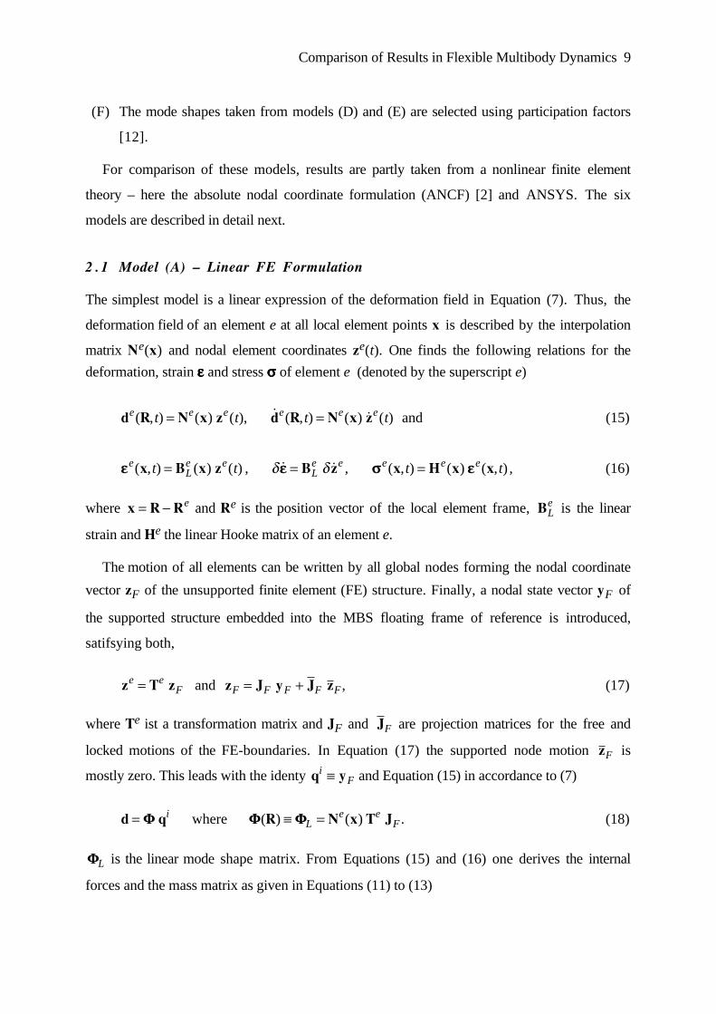
In Figure 5 the first eigenmode of the unsupported linkage is plotted, using the Buckens
frame of reference. The values of the first ten eigenfrequencies are 45.0, 96.7, 113.0, 118.2,
202.4, 286.1, 335.9, 367.9, 430.5 and 521.6 Hz. To discuss the described approximations for
deformations, the linkage is constrained at various nodes and loaded by a spatial force F and
torque L at node 20, thus p20 = (Fx Fy Fz Lx Ly Lz)T. The specific load cases are listed in
Table 1.
x
y
z
1
23
4 5
67
8
9
10
11
12
1314
15 16
17
18
19
20
21
wheel carrier car body
stabilisation linkage
Figure 4. FE-mesh of the stabilisation linkage.
16 O. Wallrapp and S. Wiedemann
y
x
1234
5 67 8
910 11
121314
15 16
1718
1920
Mode 1, 45.0 Hz
Figure 5. First eigenmode of the unsupported linkage.
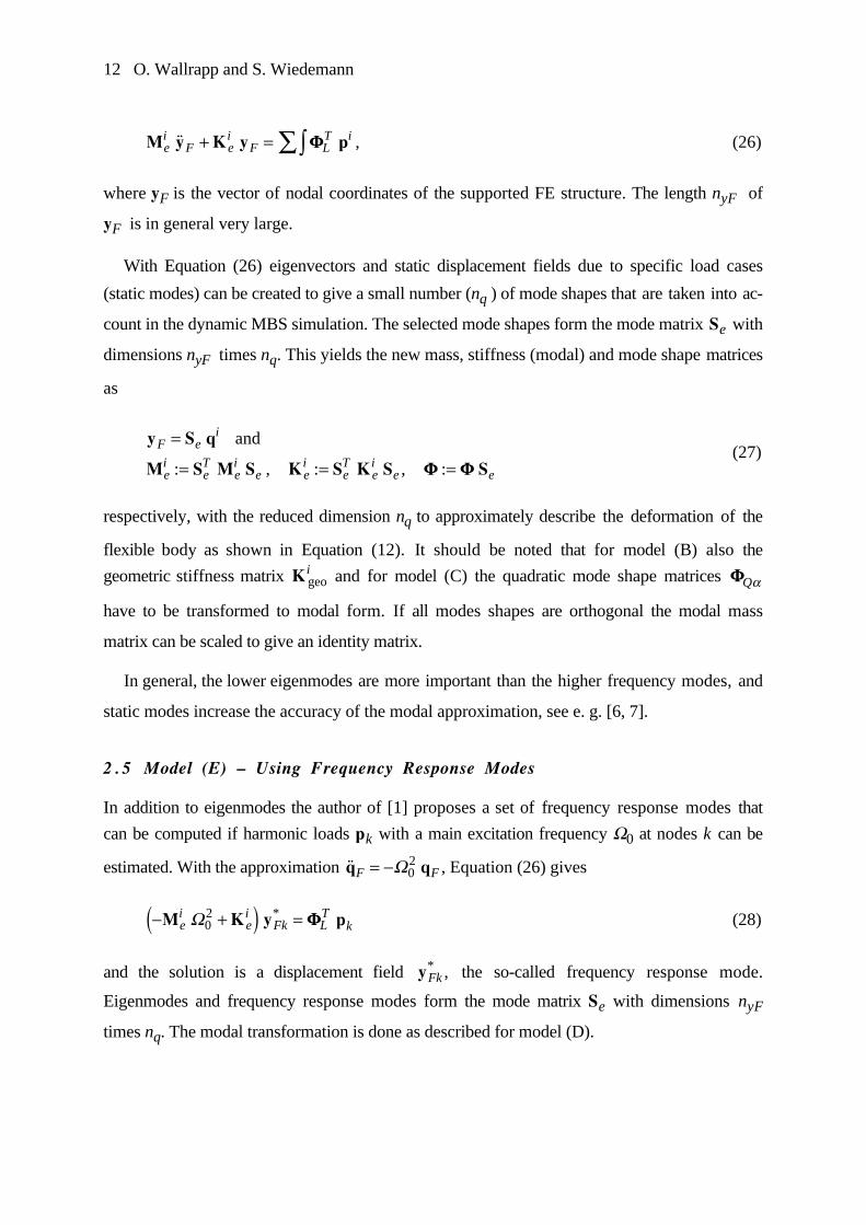
Linear vs. quadratic approximation
To discuss the effects of a quadratic approximation field of the deformation, the linkage is
analysed for load cases 1, 2 and 3. For load case 3 the deformed and undeformed linkage are
plotted in Figure 6. Table 2 lists the results of the displacements at node 20, d20 = (ux uy uz Jx
Jy Jz)T. Here the results obtained with the ANCF method serves as the reference solution with
360 DOF's. For comparison, nonlinear ANSYS results of a model with 600 DOF's are also
given in Table 2.
For the three load cases, the error of the linear model (A) for the displacement uy is very
large. With a growing force (compare case 1 and case 2) also other displacements show errors
larger than 3 %. Model (C) dramatically reduces the errors for load case 2 from 33 % to 3.5 %.
This implies that the quadratic approximation of the deformation field is a powerful model to
describe deformations far beyond the linear case. However, for load case 3 the linkage is
largely deformed due to the quadratic formulation, see Fig 6.
-0.75 -0.5 -0.25 0 0.25 0.5 0.750
0.2
0.4
y
z
12 3
45
6 7 8 910 11
12 1314 15161718 19
20
Figure 6. Deformation of the linkage for load case 3.
Comparison of Results in Flexible Multibody Dynamics 17
Nodal vs. modal approximation and mode selection
In the following simulations the modal approximation with a model reduction is applied. With
the modelling options in SIMBEAM and SIMPACK, eigenmodes of the unsupported linkage
with a Buckens frame of reference are prepared. It should be noted that for the modal
formulation the linkage suspension (six constraints) has to satisfy Equation (1). The six
coordinates of the reference frame must be included in the equations of motion, Equation (3),,
together with six Lagrange multipliers representing the constraints. The number of DOF's is
thus nq + 12. For all models a linear theory of deformation is applied, but body reference
motions are computed nonlinearly in SIMPACK.
Besides a simple truncation of higher eigenmodes, a mode selection using participation
factors as described in section 2.6 is applied. For load case 2 a graph of factors is plotted in
Figure 7. In the fist case, these19 eigenmodes are selected: 1 to 10, 12 to 16, 18, 26, 26, and
27. For load case 3 and 4 with other constraints, a new set of eigenmodes is prepared using
participation factors: 14 eigenmodes with the numbers 1 to 6, 8, 9, 11, 12, 14, 16, 26, and 27
are used.
To increase the accuracy of the results, two sets of frequency response modes for an
excitation frequency of W0 = 20 Hz with forces at nodes 1 and 20 for load case 2 and at nodes
1, 7, 14 and 20 for load cases 3 and 4 are prepared using Equation (27), in addition to a few
number of eigenmodes. The simulation results are listed in Table 3. To test the mode selection
for dynamical models, a harmonic load function (load case 4) is applied. Figure 8 shows the
computed displacements uy and uz (t).
Since the linkage is a 3-dimensional structure, all bending and torsion modes are excited by
loads at node 20. Thus only a wide range of eigenmodes can describe the deformation of the
body correctly, as shown by the participation factors in Figure 7. It is seen that modes 11 and
17 are not important for the load case 2, whereas modes 26 and 27 are. From Equation (32), an
error of -10 % is estimated for displacement ux at node 20. This value is near by -11 % found
by SIMPACK, see Table 3, laod case 2, model approximation 19 em-pf.
A mode selection using participation factors for load case 2 reduces the error from 46 % to
20 % at maximum with respect to the nonlinear results. This mode set needs 100 times less
CPU time for load case 4 than the full model with 114 modes while the displacements are

18 O. Wallrapp and S. Wiedemann
similar, see Figure 8. A set with 9 modes allows for main deformations but cannot correctly
represent y-motion. Table 3 and Figure 8 also show that even using only 3 eigen-modes
together with 12 frequency response gives results in close agreement to the reference of the full
model. The reason is that the frequency response modes are a mixture of both static and
dynamic modes and account for correct boundary conditions.
0 10 20 30 40 50 60 70 80
0.1
1.0
10.0
100.0
for ux at Node 20
Participation Factors in %
Mode Number
for y at Node 20
Figure 7. Participation factors of the linkage for load case 2.
t [s]
uy 3em+12frm
uy 15em-pfuy 114em
uy 9em-pf
0.00 0.25 0.50 0.75 1.00
0.50
0.00
–0.50
–1.00
–1.50
[m] *
10–
3
uz 3em+12frm
uz 15em-pf
t [s]
uz 114emuz 9em-pf
0.00 0.25 0.50 0.75 1.00
6.0
4.5
–1.5
–3.0
–6.0
3.0
1.5
0.0
–4.5
[m] *
10–
2
Figure 8. Displacements ux and uz of the linkage at node 20 for load case 4.
em = eigenmodes, pf = selected using participation factors, frm = frequency response modes.
Comparison of Results in Flexible Multibody Dynamics 19
4. Simulation of the Deployment of a Solar Array
Due to the complexity of this model as shown in Figure 2 and the fact that about 500 real time
seconds must be covered, time simulations using nodal coordinates to serve as a reference for
the true deformations or their best approximations cannot be made in a sensible amount of time.
Consequently only a modal representation of the deformation of the flexible bodies can be
applied.
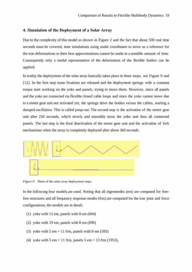
In reality the deployment of the solar array basically takes place in three steps, see Figure 9 and
[12]. In the first step some fixations are released and the deployment springs with a constant
torque start working on the yoke and panels, trying to move them. However, since all panels
and the yoke are connected via flexible closed cable loops and since the yoke cannot move due
to a motor gear unit not activated yet, the springs drive the bodies versus the cables, starting a
damped oscillation. This is called jump-out. The second step is the activation of the motor gear
unit after 250 seconds, which slowly and smoothly turns the yoke and thus all connected
panels. The last step is the final deactivation of the motor gear unit and the activation of lock
mechanisms when the array is completely deployed after about 360 seconds.
Figure 9. Shots of the solar array deployment steps.
In the following four models are used. Noting that all eigenmodes (em) are computed for free-
free structures and all frequency response modes (frm) are computed for the true joint and force
configurations, the models are in detail:
(1) yoke with 15 em, panels with 8 em (604)
(2) yoke with 19 em, panels with 8 em (690)
(3) yoke with 5 em + 11 frm, panels with 8 em (583)
(4) yoke with 5 em + 11 frm, panels 5 em + 13 frm (1953),
20 O. Wallrapp and S. Wiedemann
where the brackets give the necessary CPU time in seconds.
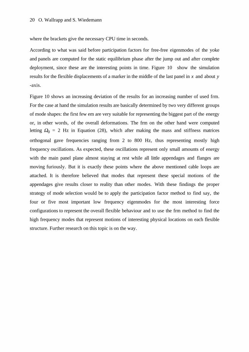
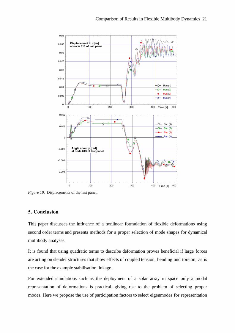
According to what was said before participation factors for free-free eigenmodes of the yoke
and panels are computed for the static equilibrium phase after the jump out and after complete
deployment, since these are the interesting points in time. Figure 10 show the simulation
results for the flexible displacements of a marker in the middle of the last panel in x and about y
-axis.
Figure 10 shows an increasing deviation of the results for an increasing number of used frm.
For the case at hand the simulation results are basically determined by two very different groups
of mode shapes: the first few em are very suitable for representing the biggest part of the energy
or, in other words, of the overall deformations. The frm on the other hand were computed
letting W0 = 2 Hz in Equation (28), which after making the mass and stiffness matrices
orthogonal gave frequencies ranging from 2 to 800 Hz, thus representing mostly high
frequency oscillations. As expected, these oscillations represent only small amounts of energy
with the main panel plane almost staying at rest while all little appendages and flanges are
moving furiously. But it is exactly these points where the above mentioned cable loops are
attached. It is therefore believed that modes that represent these special motions of the
appendages give results closer to reality than other modes. With these findings the proper
strategy of mode selection would be to apply the participation factor method to find say, the
four or five most important low frequency eigenmodes for the most interesting force
configurations to represent the overall flexible behaviour and to use the frm method to find the
high frequency modes that represent motions of interesting physical locations on each flexible
structure. Further research on this topic is on the way.
Comparison of Results in Flexible Multibody Dynamics 21
0 100 200 300 400 500
0.005
0.01
0.015
0.02
0.025
0.03
0.035
0.04
0
Run (4)
Run (3)
Run (2)
Run (1)
Displacement in x [m]at node 813 of last panel
Time [s]
0 100 200 300 400 500
-0.003
-0.002
-0.001
0
0.001
0.002
Run (4)
Run (3)
Run (2)
Run (1)
Angle about y [rad]at node 813 of last panel
Time [s]
Figure 10. Displacements of the last panel.
5. Conclusion
This paper discusses the influence of a nonlinear formulation of flexible deformations using
second order terms and presents methods for a proper selection of mode shapes for dynamical
multibody analyses.
It is found that using quadratic terms to describe deformation proves beneficial if large forces
are acting on slender structures that show effects of coupled tension, bending and torsion, as is
the case for the example stabilisation linkage.
For extended simulations such as the deployment of a solar array in space only a modal
representation of deformations is practical, giving rise to the problem of selecting proper
modes. Here we propose the use of participation factors to select eigenmodes for representation

22 O. Wallrapp and S. Wiedemann
of the main deformations and to use frequency response modes to represent high frequency
local flexible motions at the spots of interest. An estimation error of the deformations
displacements can be found for the reduced mode shape model with respect to a model
including all available mode shapes.
References
1. S. Dietz, Vibration and Fatigue Analysis of Vehicle Systems Using Component Modes, Berlin, Dissertation,
Fortschritt-Berichte VDI, Reihe 12: Verkehrstechnik/Fahrzeugtechnik, Nr. 401, Düsseldorf, VDI-Verlag, 1999.
2. S. v. Dombrowski, Analysis of Large Flexible Body Deformation in Multibody Systems Using Absolute
Coordinates. Multibody System Dynamics, 8, 2002, pp. 409-432.
3. C. Pösl, Erweiterung und Testen des Moduls SimBeam uner SIMPACK, Fachhochschule München, Diplom
Thesis, 2002.
4. W. Rulka, A. Eichberger, SIMPACK: An Analysis and Design Tool for Mechanical Systems, in Multibody
Computer Codes in Vehicle System Dynamics, (W. Kortüm and R. S. Sharp, ed.), Vol. 22, Supplement to
Vehicle System Dynamics, Swets and Zeitlinger, Amsterdam, 1993, pp. 122-126.
5. R. Schwertassek, O. Wallrapp, Dynamik flexibler Mehrkörpersysteme. Friedr. Vieweg Verlag,
Braunschweig, 1999.
6. R. Schwertassek, O. Wallrapp, S. v. Dombrowski, Modal Representation of Stress in Flexible Multibody
Simulation. Nonlinear Dynamics, 20(4), 1999, pp. 381-399.
7. R. Schwertassek, O. Wallrapp, A. Shabana, Flexible Multibody Simulation and Choice of Shape Functions.
Nonlinear Dynamics, 20(4), 1999, pp. 361-380.
8. A. A. Shabana, Flexible Multibody Dynamics: Review of Past and Recent Developments. Multibody
System Dynamics, 1, 1997, pp. 189-222.
9. O. Wallrapp, Standardization of Flexible Body Modeling in Multibody System Codes, Part I: Definition of
Standard Input Data. Mechanics of Structures and Machines, 22(3), 1994, pp. 283-304.
10.O. Wallrapp, Nonlinear Beam Theory in Flexible Multibody Dynamics - Theory of SIMBEAM, Intec
GmbH, Wessling, Report Version March 2002.
11.O. Wallrapp, R. Schwertassek, Representation of Geometric Stiffening in Multibody System Simulation.
Int. Journal for Numerical Methods in Engineering, 32, 1991, pp. 1833-1850.
12.O. Wallrapp, S. Wiedemann, Simulation of Deployment of a Flexible Solar Array. Multibody System
Dynamics, 7, 2002, pp. 101-125.

Comparison of Results in Flexible Multibody Dynamics 23
List of Figure Captions
Figure 1. Stabilisation linkage of a car's front suspension.
Figure 2. Deployment of a flexible solar array.
Figure 3 General model of a flexible body i.
Figure 4. FE-mesh of the stabilisation linkage.
Figure 5. First eigenmode of the unsupported linkage.
Figure 6. Deformation of the linkage for load case 3.
Figure 7. Participation factors of the linkage for load case 2.
Figure 8. Displacements ux and uz of the linkage at node 20 for load case 4.
em = eigenmodes, pf = selected using participation factors, frm = frequency response modes.
Figure 9. Shots of the solar array deployment steps.
Figure 10. Displacements of the last panel.
24 O. Wallrapp and S. Wiedemann
List of Tables
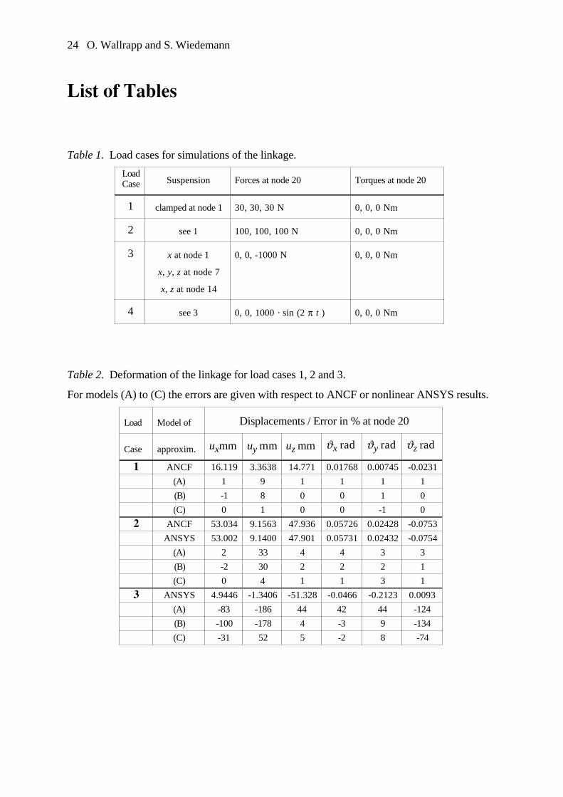
Table 1. Load cases for simulations of the linkage.
LoadCase Suspension Forces at node 20 Torques at node 20
1 clamped at node 1 30, 30, 30 N 0, 0, 0 Nm
2 see 1 100, 100, 100 N 0, 0, 0 Nm
3 x at node 1
x, y, z at node 7
x, z at node 14
0, 0, -1000 N 0, 0, 0 Nm
4 see 3 0, 0, 1000 · sin (2 p t ) 0, 0, 0 Nm
Table 2. Deformation of the linkage for load cases 1, 2 and 3.
For models (A) to (C) the errors are given with respect to ANCF or nonlinear ANSYS results.
Load Model of Displacements / Error in % at node 20
Case approxim. uxmm uy mm uz mm Jx rad Jy rad Jz rad
1 ANCF 16.119 3.3638 14.771 0.01768 0.00745 -0.0231
(A) 1 9 1 1 1 1
(B) -1 8 0 0 1 0
(C) 0 1 0 0 -1 0
2 ANCF 53.034 9.1563 47.936 0.05726 0.02428 -0.0753
ANSYS 53.002 9.1400 47.901 0.05731 0.02432 -0.0754
(A) 2 33 4 4 3 3
(B) -2 30 2 2 2 1
(C) 0 4 1 1 3 1
3 ANSYS 4.9446 -1.3406 -51.328 -0.0466 -0.2123 0.0093
(A) -83 -186 44 42 44 -124
(B) -100 -178 4 -3 9 -134
(C) -31 52 5 -2 8 -74
Comparison of Results in Flexible Multibody Dynamics 25
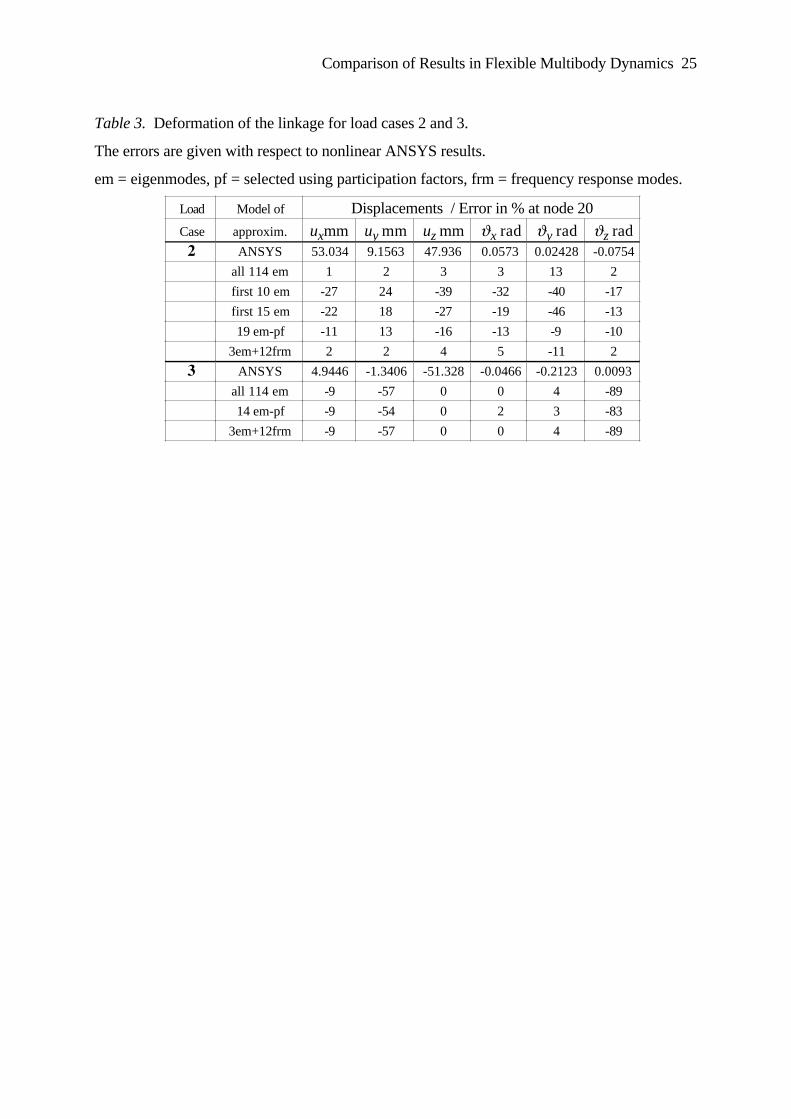
Table 3. Deformation of the linkage for load cases 2 and 3.
The errors are given with respect to nonlinear ANSYS results.
em = eigenmodes, pf = selected using participation factors, frm = frequency response modes.
Load Model of Displacements / Error in % at node 20
Case approxim. uxmm uy mm uz mm Jx rad Jy rad Jz rad2 ANSYS 53.034 9.1563 47.936 0.0573 0.02428 -0.0754
all 114 em 1 2 3 3 13 2
first 10 em -27 24 -39 -32 -40 -17
first 15 em -22 18 -27 -19 -46 -13
19 em-pf -11 13 -16 -13 -9 -10
3em+12frm 2 2 4 5 -11 2
3 ANSYS 4.9446 -1.3406 -51.328 -0.0466 -0.2123 0.0093
all 114 em -9 -57 0 0 4 -89
14 em-pf -9 -54 0 2 3 -83
3em+12frm -9 -57 0 0 4 -89