Comparison of Particle Swarm Optimization and Shuffle...

Int. J. Advance. Soft Comput. Appl., Vol. 3, No. 3, November 2011

ISSN 2074-8523; Copyright © ICSRS Publication, 2011

www.i-csrs.org

Comparison of Particle Swarm Optimization and

Shuffle Complex Evolution for Auto-Calibration of

Hourly Tank Model’s Parameters

Kuok King Kuok, Sobri Harun and Po-Chan Chiu

Lecturer, School of Engineering, Computing and Science, Swinburne University of

Technology Sarawak Campus, Jalan Simpang Tiga, 93350 Kuching, Sarawak, Malaysia

email: [email protected]

Professor, Soft Computing Research Group, Faculty of Computer Science and Information

System, Universiti Teknologi Malaysia, 81310 Skudai, Johor, Malaysia


Associate Professor, Department of Hydraulics and Hydrology, Faculty of Civil Engineering,

Universiti Teknologi Malaysia, 81310 UTM Skudai, Johor, Malaysia


Lecturer, Department of Information System, Faculty of Computer Science and Information

Technology, University Malaysia Sarawak, 94300 Samarahan, Sarawak, Malaysia

email:[email protected]

Abstract

The famous Hydrological Tank Model is always preferred for runoff forecasting. This main reason is Tank Model not only simple in term of its structures, but able to forecast runoff accurately using only rainfall and runoff data. However, much time and effort are required to calibrate a large numbers of parameters in the model for obtaining better results through trial-and-error procedure. Therefore, there is an urgent need to develop an auto-calibration method. Two types of global optimization methods (GOMs), named as Particle Swarm Optimization (PSO) and Shuffle Complex Evolution (SCE) are selected. The selected study area is Bedup basin, Samarahan, Sarawak, Malaysia. Input data used for model calibration are hourly rainfall and runoff only. The accuracy of the simulation results are measured using Coefficient of Correlation (R) and Nash-Sutcliffe Coefficient (E

2). The robustness of the

model parameters obtained are further analyzed with boxplots analysis. Peak errors are also evaluated to determine the difference between the observed and simulated peaks. Results revealed that the performance of simple PSO method is slightly better than the famous and complicated SCE method. PSO is able to obtain optimal values for 10 parameters fast and accurate within a multidimensional parameter space that could provide the best fit between the observed and simulated runoff.

Kuok, K.K et. al,

2

Keywords: Hydrological Tank Model, particle swarm optimization (PSO), shuffle complex evolution (SCE), rainfall-runoff model.

1 Introduction

There are many deterministic and conceptual models that are able to simulate daily

and hourly runoff accurately. However, most of them have complex structures and required

various types of data. Thus, Hydrological Tank Model that considered the watershed as a

series of storage vessels is selected in this study. This simple structure requires only rainfall

and runoff data for model calibration.

Tank Model was first proposed by Sugawara and Funiyuki (1956). According to Paik

et al. (2005), despite the simple structure, Tank Model has proven more capable than many

other models in modeling the hydrologic responses from a wide range of humid watersheds

(World Meteorological Organization, 1975; Franchini and Pacciani, 1991).

However, the major work in applying this hydrological model is fitting the model parameters.

In early days, the most common procedure for searching the model parameters is through

trial-and-error procedure. This manual calibration process is tedious and time consuming

owing to the large numbers of model parameters involved in the four-layered Tank Model.

Sometimes, the simulation results may be uncertain due to the subjective factors involved.

Therefore, this study is carried out to determine a more efficient automatic calibration

procedure. Recently, various optimization techniques have been developed (Shuchita and

Richa, 2009; Rahnama and Jahanshai, 2009; Premalatha and Natarajan, 2010a)

Past studies claimed that the most effective and efficient GOM for auto-calibration of

Tank Model is shuffle complex evolution (SCE) (Cooper et al., 1997; Chen et al., 2005).

Cooper et al. (2007) extended the SCE optimization technique by including hydrologic

process-based parameter constraints to improve the accuracy and efficiency of calibration

procedures. Meanwhile, the most frequent algorithm investigated is GA where Cooper et al.

(1997), Paik et al. (2005), Chen and Barry (2006) have compared the performance of GA

with other algorithms even though GA is not always the best algorithm. Other algorithms

such as simulated annealing (SA), Standardized Powell Method (SP), Marquardt algorithm,

Multistart Powell, modified harmony search algorithm (MHS), Rosenbrock algorithm and

simplex technique are rarely used by the researchers.

Due to the superiority and popularity of SCE methods, this method is selected to auto-

calibrate the Tank Model parameters in humid region that consists of four storage vessels.

The performance of SCE method is then compared with particle swarm optimization method

(PSO), a simple and newly developed optimization algorithm, but has proven it realization

and promising optimization ability in solving various problems (Song and Gu, 2004).

Currently, the application of PSO method in hydrology is still rare. Alexandre and

Darrel (2006) applied multiobjective particle swarm optimization (MOPSO) algorithm for

finding nondominated (Pareto) solutions when minimizing deviations from outflow water

quality targets. Bong and Bryan (2006) used PSO to optimize the preliminary selection,

sizing and placement of hydraulic devices in a pipeline system in order to control its transient

response. Janga and Nagesh (2007) used multiobjective particle swarm optimization

(MOPSO) approach to generate Pareto-optimal solutions for reservoir operation problems.

Subashini and Bhuvaneswari (2011) applied non-dominated sorting particle swarm

optimization (NSPSO) to combine the operations of NSGA–II for scheduling tasks in a

heterogeneous environment. Premalatha and Natarajan (2010b) hybrid PSO and Genetic

Algorithm (GA) approaches for solving the document clustering problem.

3

2 Study Area

The selected study area is

City, Sarawak, Malaysia. It is non

Batang Sadong. The basin area is approximately about 47.5km

8m to 686m above mean sea level (JUPEM, 1975). Vegetation cover

plant and forest. The development and land use changes are not really significant in this rural

watershed for the past 30 years. Sungai Bedup's basin has a dendriti

Maximum stream length for the basin is approximately 10km, which is measured from the

most remote area point of the stream to the basin outlet.

The locality plan of Bedup

Sadong basin. Main boundary of the Sadong

within Sadong basin, are shown in Fig. 1b.

available in Bedup basin, namely, Bukit Matuh (BM), Semuja Nonok (SN), Sungai Busit

(SB), Sungai Merang (SM) and Sungai Teb (ST), and one river stage gauging station at

Sungai Bedup located at the outlet of the basin.

Soil map of Bedup basin

covered with clayey soil, such as

(Bjt) and Anderson (And). Clayey soil has low infiltration rate (minimum infiltration rate of

0.04 inches/hr), where most of the precipitation fails to infiltrate

and thus produces surface runoff. Part of Bedup

(Trh), Semilajau (Sml) soils, which are coarse loamy soil. This group of soil has higher

infiltration rate (minimum infiltration rate of 1.02 inches/hr) and therefore has moderately

low runoff potential.

Sadong River

b) Sadong basin and river network (DID, 2004)

Comparison of Particle Swarm Optimization

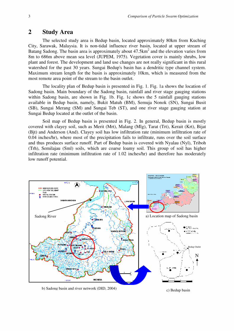
The selected study area is Bedup basin, located approximately 80km from Kuching

City, Sarawak, Malaysia. It is non-tidal influence river basin, located at upper stream of

Batang Sadong. The basin area is approximately about 47.5km2 and the elevation varies

8m to 686m above mean sea level (JUPEM, 1975). Vegetation cover is mainly shrubs, low


watershed for the past 30 years. Sungai Bedup's basin has a dendritic type channel system.


most remote area point of the stream to the basin outlet.The

The locality plan of Bedup basin is presented in Fig. 1. Fig. 1a shows the location of

asin. Main boundary of the Sadong basin, rainfall and river stage gauging stations

are shown in Fig. 1b. Fig. 1c shows the 5 rainfall gauging stations

namely, Bukit Matuh (BM), Semuja Nonok (SN), Sungai Busit


Sungai Bedup located at the outlet of the basin.

asin is presented in Fig. 2. In general, Bedup

such as Merit (Mrt), Malang (Mlg), Tarat (Trt),

Clayey soil has low infiltration rate (minimum infiltration rate of

most of the precipitation fails to infiltrate, runs over the soil surface

surface runoff. Part of Bedup basin is covered with Nyalau

, which are coarse loamy soil. This group of soil has higher

filtration rate (minimum infiltration rate of 1.02 inches/hr) and therefore has moderately

a) Location map of Sadong basin

b) Sadong basin and river network (DID, 2004) c) Bedup basin


, located approximately 80km from Kuching

tidal influence river basin, located at upper stream of

and the elevation varies from

mainly shrubs, low


c type channel system.


presented in Fig. 1. Fig. 1a shows the location of

asin, rainfall and river stage gauging stations

Fig. 1c shows the 5 rainfall gauging stations

namely, Bukit Matuh (BM), Semuja Nonok (SN), Sungai Busit


in Fig. 2. In general, Bedup basin is mostly

, Kerait (Krt), Bijat

Clayey soil has low infiltration rate (minimum infiltration rate of

runs over the soil surface

Nyalau (Nyl), Triboh

, which are coarse loamy soil. This group of soil has higher

filtration rate (minimum infiltration rate of 1.02 inches/hr) and therefore has moderately

N

Bedup Outlet

a) Location map of Sadong basin

c) Bedup basin

Kuok, K.K et. al,

4

Fig 1: Locality map of Bedup basin, Sub-basin of Sadong basin, Sarawak

Fig. 2: Soil Map of Bedup basin, Sarawak (DOA, 1975)

The input data used is hourly rainfall data from the 5 rainfall stations. Data series used

for model calibration and verification are hourly rainfall and runoff from year 1990 to year

2003 obtained from Thiessen Polygon Analysis. The area weighted precipitation for BM, SN,

SB, SM, ST are found to be 0.17, 0.16, 0.17, 0.18 and 0.32 respectively. The average areal

hourly rainfall data for that time step is then fed into the Tank Model. The calibrated Tank

Model will then carry out computations to simulate the hourly discharges for Bedup outlet.

Observed runoff data are converted from water level data through a rating curve given by

Equation 1 (DID, 2004).

Q=9.19( H )1.9

(1)

where Q is the discharge (m3/s) and H is the stage discharge (m). These observed runoff data

were used to compare the model runoff.

3 Global Optimization Methods (GOMs)

Two types of GOMs namely SCE and PSO methods are selected for auto-calibration

of hourly Tank Model’s parameters. The details of these two algorithms are described below.

3.1 Particle Swarm Optimization (PSO) Method

Particle swarm optimization (PSO) was developed by Kennedy and Eberhart (1995).

PSO is initialized with a group of random particles (trial solutions), which are assigned with

random positions and velocities. The algorithm then searches for optima through a series of

iterations where the particles are moved through the hyperspace searching for potential

solutions. These particles “learn” over time in response to their own experience and those of

other particles in their group (Ferguson, 2004).

N

Mrt/Nyl

Trt/Rmn

Mrt/Mlg/Bj

Mrt

Mrt/Krt

Trh/Smi

And

Nyl

Mrt/Trh

5 Comparison of Particle Swarm Optimization

According to Eberhart and Shi (2001), each particle keeps track of its best fitness

position in hyperspace that it has achieved so far. This best position value is called personal

best or “pbest”. The overall best value obtained by any particle so far in the population is

called global best or “gbest”. During each iterations, every particle is accelerated towards its

own “pbest” as well as in the direction of the “gbest” position. This is achieved by calculating

a new velocity term for each particle based on the distance from its “pbest” as well as its

distance from the “gbest” position. These two “pbest” and “gbest” velocities are then

randomly weighted to produce the new velocity value for this particle, which will affect the

next position of the particle in next iteration (Van den Bergh and Engelbrecht., 2000). The

basic PSO procedure is presented in Fig. 3.

Jones (2005) specified two equations used in PSO, named as movement equation

(Equation 2) and velocity update equation (Equation 3). Movement equation provides the

actual movement of the particles using their specific vector velocity while the velocity

updates equation provides for velocity vector adjustment given the two competing forces

(“gbest” and “pbest”). Besides, inertia weight (ω) was introduced to improve the convergence

rate (Shi and Eberhart, 1998).

Fig. 3: Basic PSO procedure

tVonprevLocationpresLocati i∆+= (2)

Vi =ωVi-1 + c1*rand()*(pbest-presLocation) +c2*rand()*(gbest-presLocation) (3)

Meet Stopping Criteria

Nex

t P

arti

cle

No

Exit Criteria

(Global Best

Satisfactory)

Randomly Initialize Population Locations and Velocities

Evaluate Fitness of Particle

If Particle Fitness > Global Best Fitness

Update Global Best

If Particle Fitness > Particle Best Fitness

Update Particle Best

Update Particle Velocity

Update Particle Position

“gbest”

“pbest”

YES

Kuok, K.K et. al,

6

where Vi is the current velocity, t∆ defines the discrete time interval over which the particle

will move, ω is the inertia weight, Vi-1 is the previous velocity, presLocation is the present

location of the particle, prevLocation is the previous location of the particle and rand() is a

random number between 0 and 1, c1 and c2 are the acceleration constants for “gbest” and

“pbest” respectively.

3.2 Shuffle Complex Evaluation (SCE) Method

The SCE method is a global optimization algorithm that based on a synthesis of four

concepts that have proved to be effective automatic calibration tool for optimization problems

(Duan et al., 1992). These four concepts are a) combination of random and deterministic

approaches, b) the concept of clustering, c) the concept of a systematic evolution of a

complex of points spanning the space, d) the concept of competitive evolution. The

combination of these concepts made the SCE known as a powerful, effective and flexible

method. SCE method consists of two parts, SCE and competitive complex evolution (CCE).

Fig. 4: SCE Calibration Process

For SCE method, the search within the feasible region is conducted by first dividing

the set of current feasible trial solutions into several complexes, each containing equal

number of trial solutions. Concurrent and independent searches within each complex are

conducted until each converges to its local optimal value. For each of the complexes, that are

now defined by new trial solutions is collated into a common pool, shuffled by ranking

according to their objective function value and then further divided into new complexes. The

procedure is terminated when none of the local optima found among the complexes can

improve on the best current local optimum. The SCE method used the Nelder and Mead

(1965) downhill simplex method to accomplish local searches. The flow chart of SCE

calibration process was shown in Fig. 4.

Processor 1

Complex

Evolution at t

times

Processor 2

Complex

Evolution at t

times

Processor N

Complex

Evolution at t

times

Generate Sample Population

Partition the Data into Complexes

Combine the Complexes & shuffle

Optimum Parameters

Meet Stopping Criteria No

Yes

7

The competitive complex evolution (CCE) algorithm is required for the evolution of

each complex. Each point of a complex is a potential 'pare

the process of reproducing offspring. A subcomplex functions like a pair of parents. Use of a

stochastic scheme to construct subcomplexes allows the parameter space to be searched more

thoroughly. The idea of competit

stronger survives better and breed healthier offspring than the weaker. Inclusion of the

competitive measure expedites the search towards promising regions.

4 Tank Model Parameters

Since Tank Model is developed

development or management agencies all over the world

simple and easily to understan

surface runoff (Kawasaki, 2003).

The response of surface runoff system is explained by vertically connected plural

tanks. The model consists of four storage vessels (4

one or more outlets on its side and bottom.

second storage tank (TS2) represent

tank and the forth tank (TS4) represent

occur when the water level in each tank is higher than the height of side outlet. The output

from the bottom outlet of the first tank

bottom outlets for the rest of the tanks could be regarded as percolation.

Q was calculated using Equation 4.

5.

Q= C1Q1 + C2Q2 + C4Q3 + C6Q4 + C8Q5

Fig. 5: Schematic of



ach point of a complex is a potential 'parent' with the ability to participate in


construct subcomplexes allows the parameter space to be searched more

thoroughly. The idea of competitiveness is introduced in forming subcomplexes where the


competitive measure expedites the search towards promising regions.

Tank Model Parameters

developed in 1956, it has been adopted by many water resources

development or management agencies all over the world. This is not only due to the

and, but also it is able to indicate accurately the response for

ce runoff (Kawasaki, 2003).


odel consists of four storage vessels (4-Tank) that lay vertically.

one or more outlets on its side and bottom. First storage tank (TS1) represent

second storage tank (TS2) represents intermediate tank; third tank (TS3) represent

tank and the forth tank (TS4) represents base tank. Each outflow from side outlet will only

in each tank is higher than the height of side outlet. The output

from the bottom outlet of the first tank is used to model infiltration, the outputs from the

bottom outlets for the rest of the tanks could be regarded as percolation. The total discharge,

was calculated using Equation 4. A schematic diagram of Tank Model

Q= C1Q1 + C2Q2 + C4Q3 + C6Q4 + C8Q5

Fig. 5: Schematic of Tank Model used in this study

Rainfall

Evaporation



ability to participate in


construct subcomplexes allows the parameter space to be searched more

iveness is introduced in forming subcomplexes where the


in 1956, it has been adopted by many water resources

not only due to the model is

able to indicate accurately the response for


vertically. Each tank has

storage tank (TS1) represents surface tank;

intermediate tank; third tank (TS3) represents sub-base

base tank. Each outflow from side outlet will only

in each tank is higher than the height of side outlet. The output

is used to model infiltration, the outputs from the

The total discharge,

odel is presented in Fig.

(4)

Kuok, K.K et. al,

8

Parameters of Tank Model are side outlet coefficients (C1, C2, C4, C6 and C8),

bottom outlet coefficients (C3, C5 and C7), height of side outlets (X1, X2, X3, X4 and X5)

and initial storages in tanks (TS1, TS2, TS3 and TS4). The descriptions of 10 parameters are

tabulated in Table 1. Prior to calibration, parameters X3, X4 and X5 are set to 0, This is

because these parameters have little impact to model output and the values obtained are

always near to 0. Hence, the remaining 10 parameters that calibrated automatically using

PSO and SCE algorithms are C1, C2, C3, C4, C5, C6, C7, C8, X1 and X2. The models

calibrated by PSO and SCE algorithms are denoted as PSO-Tank-H and SCE-Tank-H

respectively.

Table 1: The description of the 10 parameters for Tank Model

No Coeff Identification Description

1 C1 Side outlet coefficients No.1 for TS1 Surface runoff coefficient No.1

2 C2 Side outlet coefficients No.2 for TS1 Surface runoff coefficient No.2

3 C3 Bottom outlet coefficient from TS1 to

TS2

Infiltration coefficient from surface tank to

intermediate tank

4 C4 Side outlet coefficients for TS2 Intermediate runoff coefficient


TS3

Infiltration coefficient from intermediate tank to

sub-base tank

6 C6 Side outlet coefficients for TS3 sub-base runoff coefficient


TS4

Infiltration coefficient from sub-base tank to

base tank

8 C8 Side outlet coefficients for TS4 Base runoff coefficient

9 X1 Height of side outlets No.2 for TS1 Height of surface runoff No.2 from surface tank

10 X2 Height of side outlets No.1 for TS1 Height of surface runoff No.1 from surface tank

5 Model Calibration

The input data to Tank Model comprised of hourly average areal rainfall calculated

using Thiesen Polygon method. In order to find the most robust parameters, Tank Model is

calibrated using 11 sets of hourly rainfall-runoff data and the learning mechanism depends on

the type of algorithm applied. Each set of parameters obtained is further validated with other

11 storm hydrographs. Hence, there are 121 repetitions for each set of experiments calibrated

with PSO and SCE respectively. Table 2 presents the storm hydrographs used for finding the

optimal Tank Model’s parameters of PSO-Tank-H and SCE-Tank-H.

Table 2: Calibration data for PSO-Tank-H and SCE-Tank-H

Description Storm Date

PSOSetHA, SCESetHA 1-7 Jan 99

PSOSetHB, SCESetHB 5-8 Apr 99

PSOSetHC, SCESetHC 5-8 Feb 99

PSOSetHD, SCESetHD 8-12 Aug 98

PSOSetHE, SCESetHE 9-12 Sep 98

PSOSetHF, SCESetHF 15-18 Mac 99

PSOSetHG, SCESetHG 20-24 Jan 99

PSOSetHH, SCESetHH 26-31 Jan 99

PSOSetHI, SCESetHI 16-20 Apr 03

PSOSetHJ, SCESetHJ 18-21 Jan 00

PSOSetHK, SCESetHK 9-12 Oct 03


The robustness of the optimal parameters obtained will be further evaluated with

different sets of validation data. 11 single storm hydrographs are used to validate the hourly

simulation model. The validation data sets used for hourly runoff simulation are presented in

Table 3.

Table 3: Validation data for hourly runoff

Description Storm Date

Hydrograph 1 1-7 Jan 99

Hydrograph 2 5-8 Apr 99

Hydrograph 3 5-8 Feb 99

Hydrograph 4 8-12 Aug 98

Hydrograph 5 9-12 Sep 98

Hydrograph 6 15-18 Mac 99



Hydrograph 9 16-20 Apr 03


Hydrograph 11 9-12 Oct 03

The robustness of the validated data for hourly runoff simulation is then measured

with boxplots whiskers analysis. The objective function selected is ordinary least squares

(OLS). OLS always provide better approximations of the model parameters due to its

algebraic formulations where each of these formulations consists of a summation of the least

squares differences for every point in the flow series (Cooper et al., 1997). The objective

function will evaluate the performance of the GOMs in calibrating Tank Model and it will

ensure that the learning error is getting lesser with the increase of number iterations. The

accuracy of simulation results is measured using the coefficient of correlation (R) and Nash-

Sutcliffe coefficient (E2).

6 Performance Evaluation

Boxplots is applied to determine the robustness of parameters investigated. In its

simplest form, the boxplot presents five sample statistics namely the minimum, the lower

quartile, the median, the upper quartile and the maximum, in a visual display.

Peak runoff is evaluated for each storm hydrograph simulated by optimal

configuration of Tank Model’s parameters. Observed and simulated peaks generated by

optimal configuration of PSO-Tank-H and SCE-Tank-H approaches are compared for 11

validation data sets. The objective is to evaluate how successful the simulated runoff in

approaching the observed peak. Error between observed peak and simulated peak is

calculated using Equation 5.

%100_

__x

peakobserved

peakobservedpeaksimulatedError

−= (5)

The simulated results obtained are evaluated to determine the differences between

observed and predicted values. The accuracy of model performance is measured by

Coefficient of Correlation (R) and Nash-sutcliffe coefficient (E2). According to Lauzon et al.

(2000), the R and E2 are measuring the overall differences between observed and estimated

flow values. The closer R and E2 to 1, the better the predictions are. The formulas of these

two coefficients are presented in Table 4.

Kuok, K.K et. al,

Concept

Coefficient of Correlation

Nash-Sutcliffe Coefficient

Note : obs = observed value, pred = predicted value,

7 Results and Discussion

7.1 Particle Swarm Optimization (PSO)

The results revealed that the best parameter set is obtained using single storm event on

5 to 8 April 1998 (PSOSetHC), with optimum R and E

respectively. The optimal configuration for PSO algorithm was found to be using 100

numbers of Particles (D), 200 maximum iterations and

parameters obtained using PS

X2=0.00001, C4=0.1158, C5=

storm hydrograph calibrated by the optimal configuration of PSO algorithm

Fig. 6.

Fig. 6: Comparison between observed storm hydrograph and optimal simulated storm

hydrograph using PSO

The trend of simulated hydrograph is very close with observed runoff. However, the

simulated peak is slightly lower than observed peak. Five parameters

C8 and X1 are the dominance parameters that affect the hourly runoff generation. Other

parameters such as C2, C3, C5, C7 and X2 have little impact to hourly runoff simulation. All

the infiltration coefficient values C3, C5 and C7 are

infiltration rate for Bedup b

performance of PSOSetHC when validating 11 storm events is

Table 4: Formulas for R and E2

Name Formula

R

∑ ∑

∑−−

−−

−

−

2 ()(

)((

predobsobs

predobsobs

Sutcliffe Coefficient

E2

(

(∑

∑

−

−

−=j

i

j

i

obsobs

predobs

E2

1

Note : obs = observed value, pred = predicted value, −−

obs = mean observed values, dpre−−

= mean predicted values and j = number of values.

Results and Discussion

Particle Swarm Optimization (PSO)


(PSOSetHC), with optimum R and E2 values of 0.962 and 0.8935


numbers of Particles (D), 200 maximum iterations and c1 and c2 of 1.4. The optimal

parameters obtained using PSO are C1=0.1165, C2=0.00001, X1=0.1593,

C5=0.00001, C6=0.1208, C7=0.00001 and C8=

storm hydrograph calibrated by the optimal configuration of PSO algorithm



simulated peak is slightly lower than observed peak. Five parameters including C1, C4, C6,



the infiltration coefficient values C3, C5 and C7 are found to be 0.00001

asin, which mostly covered by clayey soil is

performance of PSOSetHC when validating 11 storm events is presented in

10

Formula

−−

−−

−

−

2)

)

predpred

dprepred

)

)obs

pred

2

2

= mean predicted values and j = number of values.


values of 0.962 and 0.8935


of 1.4. The optimal

0.1593, C3=0.00001,

C8=0.0212. The best

storm hydrograph calibrated by the optimal configuration of PSO algorithm is presented in



including C1, C4, C6,



. This indicates the

asin, which mostly covered by clayey soil is very low. The

in Table 5.

11

Table 5: Results of

Description

Storm Hydrograph 1

Storm Hydrograph 2

Storm Hydrograph 3

Storm Hydrograph 4

Storm Hydrograph 5

Storm Hydrograph 6

Storm Hydrograph 7

Storm Hydrograph 8

Storm Hydrograph 9

Storm Hydrograph 10

Storm Hydrograph 11

Average

7.2 Shuffle Complex Evolution (SCE)

The best set of parameters

(SCESetHC), with nsp1 of 75 where R and E

optimal 10 parameters optimized by SCE algorithm are C1=

X1=14.7853, C3=0.311226,

C7=0.000155 and C8=0.017274.

algorithm was shown in Fig. 7. Result reveals that the simulated peak is slightly

underestimated than observed peak.


hydrograph using SCE

Infiltration coefficient values C3, C5 and C7 are

and 0.000155 respectively. This revealed that the infiltration rate from first

high. Thereafter, there is only little infiltration for the subsequent tanks. The calibration

results revealed that 8 parameters calibrated by SCE algorithm including C1, C2, C3, C4, C6,

C8, X1 and X2 are controlling the hourly runoff ge

minor effect to hourly runoff simulation. Table 6 presents the R and E

validating 11 storm events using the SCESetHC optimal parameters.


Table 5: Results of PSOSetHC for validating 11 single storm events

SCE

R E2

Storm Hydrograph 1 0.747 0.6139






Hydrograph 7 0.832 0.6961





0.8949 0.7921

Shuffle Complex Evolution (SCE)

The best set of parameters is obtained using single storm event on 5 to 8 April 1998

(SCESetHC), with nsp1 of 75 where R and E2 yielded to 0.917 and 0.8154 respectively. The

optimal 10 parameters optimized by SCE algorithm are C1=0.57876,

0.311226, X2=6.49865, C4=0.047421, C5=5.90424e-007,

0.017274. The optimal calibrated storm hydrograph using SCE


underestimated than observed peak.

parison between observed storm hydrograph and optimal simulated storm

Infiltration coefficient values C3, C5 and C7 are found to be 0.311226

respectively. This revealed that the infiltration rate from first



C8, X1 and X2 are controlling the hourly runoff generation. In contrast, C5 and C7 have

minor effect to hourly runoff simulation. Table 6 presents the R and E

validating 11 storm events using the SCESetHC optimal parameters.


11 single storm events

obtained using single storm event on 5 to 8 April 1998

to 0.917 and 0.8154 respectively. The

0.57876, C2=0.374059,

007, C6=0.695887,

The optimal calibrated storm hydrograph using SCE


parison between observed storm hydrograph and optimal simulated storm

0.311226, 5.90424e-007

respectively. This revealed that the infiltration rate from first to second tank is



neration. In contrast, C5 and C7 have

minor effect to hourly runoff simulation. Table 6 presents the R and E2 obtained when

Kuok, K.K et. al,

12

Table 6: Results of SCESetHC for validating 11 single storm events

Description SCE

R E2












Average 0.8838 0.7372

7.3 Comparison of Two GOMS

Fig. 8 shows the average R and E2 values produced by the optimal configuration of

SCE and PSO algorithm for validating 11 storms hydrograph. The average R and E2 values

obtained by PSO algorithm are 0.8949 and 0.7921 respectively. For SCE algorithm, the

average R and E2 values obtained after validating 11 storm events are 0.8838 and 0.7372

respectively. This indicates that the parameters calibrated using PSO is more accurate than

SCE when validating 11 storm events.

Fig. 8: Comparison of optimal PSO and SCE algorithms

7.4 Comparison Between Observed Peak and Simulated Peak

The simulated peak for optimal configuration of each GOMs was compared with

observed peak. Table 7 presents the peak error (%) between observed and simulated peak

flow for PSOSetHC and SCESetHC when validating 11 storms hydrograph.


Table 7: Peak flow Error for PSOSetHC and SCESetHC

SCE-Tank-H PSO-Tank-H

Storms Observed

Peak

Simulated

Peak

Error

(%)

Observed

Peak

Simulated

Peak

Error

(%)

1998 Aug 8-12 25.75 27.61 7.24 25.75 22.73 11.71

1999 Jan 1-7 34.63 27.36 20.97 34.63 23.68 31.62

1999 Apr 5-8 18.37 16.03 12.74 18.37 13.65 25.74

1999 Feb 5-8 14.26 18.58 30.30 14.26 15.28 7.14

1998 Sep 9-12 40.40 23.20 42.57 40.40 30.21 25.22

1999Mac 15-18 13.20 16.37 23.97 13.20 13.61 3.09

1999 Jan 20-24 20.36 22.38 9.92 20.36 19.35 4.98

1999 Jan 26-31 28.37 25.05 11.72 28.37 21.71 23.48

2000 Apr 5-8 22.45 19.50 13.12 22.45 19.69 12.30

2000 Jan 18-21 22.18 20.85 5.98 22.18 16.86 23.98

2003 Oct 9-12 19.36 21.22 9.62 19.36 17.27 10.78

Average Error 17.10 16.37

It was found that average error (%) between simulated and observed peak for optimal

configuration of SCE and PSO are 17.10% and 16.37% respectively. The results revealed that

PSO approach has produced simulated peaks that are closer to observed peak than SCE

approach. These simulated peaks can be used as early warning flow forecaster to take

necessary flood protection measures before a severe flood occurs.

7.5 Boxplots Analysis

To ensure the parameters obtained is the most optimal and accurate, 11 sets of storm

hydrographs are calibrated and optimized by PSO and SCE algorithms. Each set of parameter

obtained is then validated with another 11 sets of storm events. The resulting parameters

obtained using PSO and SCE calibration methods for different dataset are presented in Table

8 and 9 respectively.

Table 8: Optimal parameters obtained using PSO algorithm with different dataset

C1 C2 X1 C3 X4 C4 C5 C6 C7 C8 PSOSetHA 0.1165 0.00001 0.1593 0.00001 0.00001 0.1158 0.00001 0.1208 0.00001 0.0212

PSOSetHB 1.1435 1.1448 0.3693 0.2980 0.3232 2.4044 0.3188 0.0260 0.00001 0.0351

PSOSetHC 1.0688 1.0113 0.1393 0.00001 0.00001 1.8834 1.6107 0.0337 0.00001 0.0352

PSOSetHD 0.1087 0.00001 0.3801 0.00001 0.00001 1.3865 0.9869 0.1004 0.00001 0.0160

PSOSetHE 0.6970 0.0061 0.0011 0.00001 0.0321 2.3341 0.4037 0.0868 0.00001 0.0150

PSOSetHF 0.1561 0.00001 0.0504 0.00001 0.0003 1.8585 0.00001 0.1666 0.00001 0.0143

PSOSetHG 1.8862 0.6467 0.0744 0.00001 0.00001 1.0000 0.7005 1.0000 0.0924 0.0053

PSOSetHH 1.1934 0.00001 0.3576 0.00001 0.00001 2.3606 0.7823 0.0323 0.00001 0.0414

PSOSetHI 0.9851 0.3346 0.00001 0.0592 0.00001 1.2972 0.7070 0.0979 0.00001 0.0138

PSOSetHJ 0.1422 0.00001 0.00001 0.0008 0.00001 0.9962 1.7252 0.1686 0.00001 0.0242

PSOSetHK 0.9440 0.4144 1.0077 0.3297 0.6356 1.0000 0.6417 0.0981 0.00001 0.0127

Table 9: Optimal parameters obtained using SCE algorithm with different dataset

C1 C2 X1 C3 X4 C4 C5 C6 C7 C8 SCESetHA 0.57876 0.374059 14.7853 0.311226 6.49865 0.047421 5.90E-07 0.695887 0.000155 0.017274

SCESetHB 0.239367 0.000152 19.9981 0.00404 4.21419 0.99953 0.142576 0.999998 0.651766 0.01605

SCESetHC 0.382111 0.013735 13.3852 0.000111 10.9231 0.073761 9.38E-07 0.850929 0.00194 0.024017

SCESetHD 0.73823 0.073409 3.3418 3.13E-05 7.1593 0.42368 3.52E-06 1.000000 0.39497 0.009329

SCESetHE 0.835835 0.289136 13.3096 0.255264 12.7314 0.115417 6.29E-08 0.759014 3.18E-08 0.015798

SCESetHF 0.137185 1.65E-05 9.46114 0.880488 19.9992 0.787643 0.000103 0.716401 0.004526 0.010075

SCESetHG 0.278742 0.531293 19.3113 0.234886 19.9882 0.710385 0.000219 0.999999 0.935953 0.009887

SCESetHH 0.548313 0.480161 10.9885 0.534595 9.90657 0.999945 0.15776 0.99975 0.316135 0.018535

SCESetHI 0.660371 0.349439 15.1549 0.168425 4.16672 0.928385 2.80E-05 0.999984 0.138532 0.01006

SCESetHJ 0.113613 0.001223 19.9952 0.459864 19.1121 0.204836 1.07E-05 0.926352 0.493893 0.018574

SCESetHK 0.27012 0.164622 19.9984 0.062928 11.568 0.999998 0.152339 0.999982 0.99596 0.008362

Kuok, K.K et. al,

14

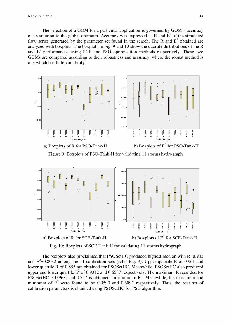
The selection of a GOM for a particular application is governed by GOM’s accuracy

of its solution to the global optimum. Accuracy was expressed as R and E2 of the simulated

flow series generated by the parameter set found in the search. The R and E2 obtained are

analyzed with boxplots. The boxplots in Fig. 9 and 10 show the quartile distributions of the R

and E2

performances using SCE and PSO optimization methods respectively. These two

GOMs are compared according to their robustness and accuracy, where the robust method is

one which has little variability.

a) Boxplots of R for PSO-Tank-H b) Boxplots of E2 for PSO-Tank-H.

Figure 9: Boxplots of PSO-Tank-H for validating 11 storms hydrograph

a) Boxplots of R for SCE-Tank-H b) Boxplots of E2 for SCE-Tank-H

Fig. 10: Boxplots of SCE-Tank-H for validating 11 storms hydrograph

The boxplots also proclaimed that PSOSetHC produced highest median with R=0.902

and E2=0.8032 among the 11 calibration sets (refer Fig. 9). Upper quartile R of 0.961 and

lower quartile R of 0.855 are obtained for PSOSetHC. Meanwhile, PSOSetHC also produced

upper and lower quartile E2 of 0.9312 and 0.6587 respectively. The maximum R recorded for

PSOSetHC is 0.968, and 0.747 is obtained for minimum R. Meanwhile, the maximum and

minimum of E2

were found to be 0.9590 and 0.6097 respectively. Thus, the best set of

calibration parameters is obtained using PSOSetHC for PSO algorithm.

2

2


Fig. 10 presents the boxplots produced by SCE algorithm. The results clearly

indicated that the best calibration set for SCE algorithm is SCESetHC among the 11

calibration sets, with median R of 0.917 and median E2 of 0.7557. The upper and lower

quartile recorded for R is 0.933 and 0.788 respectively for SCESetHC, where else 0.8418 and

0.6390 are obtained for E2. The maximum and minimum of R are found to be 0.964 and

0.765 respectively, while maximum and minimum values recorded for E2 are 0.9291 and

0.5138 respectively.

Between the two GOMs, PSO method appeared to consistently give a remarkable

performance and is considered as more robust and accurate than SCE method. PSO still

consider more reliable that SCE, even though the median of R=0.902 provided is slightly

lower than SCE method (R=0.917). This is because PSO method has produced median of

E2=0.8032, which is much better than SCE method (E

2=0.7557). Besides, boxplots also

revealed that PSO method has smaller variability for both R and E2 than SCE approach.

Moreover, average R and E2 obtained for PSO when validating 11 storms hydrograph are

higher than SCE approach (refer Fig. 8). Therefore, PSO approach performs better than SCE

for hourly runoff simulation in this study.

8.0 Conclusion

The new PSO algorithm and the famous SCE are compared to determine their

suitability and accuracy for calibration of Tank Model, under various modeling scenarios.

Both GOMs had confirmed their abilities to calibrate and optimize 10 parameters of

Hydrologic Tank Model. Optimal PSO calibration method had achieved average R=0.8949

and E2=0.7921 with the model configuration of c1=1.4, c2=1.4, 100 of number of particles,

200 max iteration when validating 11 storms hydrograph. Meanwhile, the performance of

SCE method is slightly lower than PSO with average R and E2 of 0.8838 and 0.7372

respectively for validating 11 storms hydrographs.

These results proved that the newly developed PSO algorithm has the ability to

calibrate and optimize 10 parameters of Tank Model accurately. Besides, PSO had shown its

robustness by simulating accurately the 11 single storms hydrograph during the validation

period. This indicates that PSO optimization search method is a simple algorithm, but found

to be robust, efficient and effective in searching optimal Tank Model parameters. This was

totally revealed by the ability of PSO methods in searching the optimal parameters that

provide the best fit between observed and simulated flows.

The methodology has been tested for rural catchment in humid region. The results

revealed that Hydrologic Tank Model clearly manage to demonstrate the ability to adapt to

the respective lag time of each gauge through calibration. Rainfall and runoff as inputs are

sufficient to develop an accurate hourly rainfall-runoff model. Inclusion of more parameters

such as temperature, moisture content, evaporation will make the Tank Model unnecessarily

complex in nature without any significant improvement in performance.

Kuok, K.K et. al,

16

References

[1] Alexandre, M. B. and Darrell, G. F., “A Generalized Multiobjective Particle Swarm

Optimization Solver for Spreadsheet Models: Application to Water Quality”,

Hydrology Days 2006, (2006), pp 1-12.

[2] Bong, S. J. and Bryan, W. K., “Hydraulic Optimization of Transient Protection

Devices Using GA and PSO Approaches”, Journal of Water Resources Planning and

Management © ASCE, (2006), pp 44-54

[3] Chen, J.Y., and Barry, J. A., “Semidistributed Form of the Tank Model Coupled with

Artificial Neural Networks”, Journal of Hydrologic Engineering, Vol. 11, No. 5,

(2006), pp 408-417

[4] Chen, R.S., Pi, L.C., and Hsieh, C.C., “A Study on Automatic Calibration of

Parameters in Tank Model”, Journal of the American Water Resources Association

(JAWRA), (2005).

[5] Cooper, V.A., Nguyen, V-T-V. and Nicell, J.A., “Evaluation of Global Optimization

Methods for Conceptual Rainfall-Runoff Model Calibration”, Water Sci. Technol.

36(5), (1997), pp 53-60.

[6] Cooper, V., Nguyen, V-T-V. and Nicell, J., “Calibration of Conceptual Rainfall-

Runoff Models using Global Optimization Methods with Hydrologic Process-based

Parameter Constraints”, Journal of Hydrologic, Vol. 334, No. 3-4, (2007), pp 455-

466.

[7] DID, Hydrological Year Book Year 2004, Department of Drainage and Irrigation

Sarawak, Malaysia, (2004).

[8] DOA, Jabatan Pertanian Malaysia, Scale 1:50,000, (1975).

[9] Duan, Q., Gupta, V. K., and Sorooshian, S., “Effective and Efficient Global

Optimization for Conceptual Rainfall-Runoff Models”, Water Resour. Res. 28,

(1992), pp 1014–1015.

[10] Eberhart, R. and Shi, Y., “Particle Swarm Optimization: Developments, Application

and Resources”, IEEE, (2001) 81-86

[11] Ferguson, D., Particle Swarm. University of Victoria, Canada.(2004).

[12] Franchini M, and Pacciani M., “Comparative analysis of several conceptual rainfall-

runoff models”, Journal of Hydrology 122, (1991), pp 161–219.

[13] Janga, M. R. and Nagesh, D. K., “Multi-Objective Particle Swarm Optimization for

Generating Optimal Trade-Offs in Reservoir Operation”, Hydrological Processes. 21.

(2007), pp 2897–2909.

[14] Jones M.T, AI Application Programming. 2nd Ed. Hingham, Massachusetts, (2005).

[15] JUPEM, Jabatan Ukur dan Pemetaan Malaysia. Scale 1:50,000, (1975).

[16] Kawasaki, R., “Application of Synthetic Tank Model Simulation on the Area with

Poor Basic Hydrological Data Availability”, Japan Society of Shimanto Policy and

Integrated River Management, Vol 2-2, (2003), pp 18-19.

[17] Kennedy, J. and Eberhart, R., “Particle Swarm Optimization”, Proceedings IEEE Int’l

Conf. on Neural Networks (Perth, Australia), IEEE Service Center, Piscataway, NJ,

IV, 1995), pp 1942-1948.

[18] Lauzon, N., Rousselle, J., Birikundavyi, S., and Trung, H.T., “Real-time Daily Flow

Forecasting Using Black-box Models, Diffusion Processes and Neural Networks”,

Can. J. Civ. Eng. 27, (2000), pp 671-682.

[19] Premalatha, K. and Natarajan, A.M., “Combined Heuristic Optimization Techniques

for Global Minimization”, Int. J. Advance. Soft Comput. Appl., Vol. 2, No. 1,

(2010a), pp 85-99.


[20] Premalatha, K., and Natarajan, A.M., “Hybrid PSO and GA Models for Document

Clustering”, Int. J. Advance. Soft Comput. Appl., Vol. 2, No. 3, (2010b), pp 302-320.

[21] Nelder, J.A., and Mead, R., “A Simplex Method for Function Minimization”,

Computer Journal, Vol. 7, (1965), pp. 308-313.

[22] Paik, K., Kim, J.H., and Lee, D.R.. “A Conceptual Rainfall-runoff Model Considering

Seasonal Variation”, Wiley InterScience 19, (2005), pp 3837-3850.

[23] Rahnama, M. B., and Jahanshai, P., “Water Delivery Optimization Program, of Jiroft

Dam Irrigation Networks by Using Genetic Algorithm”, Int. J. Advance. Soft

Comput. Appl., Vol. 1, No. 2, (2009), pp 151-161.

[24] Shi, Y. and Eberhart, R., “A Modified Particle Swarm Optimizer”, Proceedings of the

105 IEEE Congress on Evolutionary Computation, (1998), pp 69–73.

[25] Shuchita, U., and Richa, S., “Ant Colony Optimization: A Modified Version”, Int. J.

Advance. Soft Comput. Appl., Vol. 1, No. 2, (2009), pp 77-90.

[26] Song, M.P. and Gu, G.H., “Research on Particle Swarm Optimization: A Review”,

Proceedings of the Third International Conference on Machine Learning and

Cybernectics. Shanghai, China, (2004).

[27] Subashini, G., and Bhuvaneswari, M.C., “Non Dominated Particle Swarm

Optimization For Scheduling Independent Tasks On Heterogeneous Distributed

Environments”, Int. J. Advance. Soft Comput. Appl., Vol. 3, No. 1, (2011), pp 1-17.

[28] Sugawara M and Funiyuki M., “A Method of Revision of the River Discharge by

Means of a Rainfall Model”, Collection of Research Papers about Forecasting

Hydrologic variables, (1956), pp 14-18.

[29] Van den Bergh, F. and Engelbrecht, A. P., “Cooperative Learning in Neural Networks

using Particle Swarm Optimizers”, South African Computer Journal, (26), (2000), pp

84-90.

[30] World Meteorological Organization, “Intercomparison of conceptual models used in

operational hydrological forecasting”, Operational Hydrology Report No. 7, (1975),

WMO, Geneva, Switzerland.

Comparison of Particle Swarm Optimization and Shuffle...

Documents

Transcript of Comparison of Particle Swarm Optimization and Shuffle...