Purdue UniversityPurdue e-PubsInternational High Performance BuildingsConference School of Mechanical Engineering

2016

Comparison of Model Predictive Controlperformance using grey-box and white boxcontroller modelsDamien PicardKU Leuven, Department of Mechanical Engineering, Leuven, Belgium, damien.picard@kuleuven.be

Maarten SourbronKU Leuven, Department of Mechanical Engineering, Leuven, Belgium, maarten.sourbron@kuleuven.be

Filip JorissenKU Leuven, Department of Mechanical Engineering, Leuven, Belgium, filip.jorissen@kuleuven.be

Ji?í CiglerFeramat Cybernetics s.r.o., Czech Republic, cigler@feramat.cz

Zden?k Vá?aFeramat Cybernetics s.r.o., Czech Republic, vana@feramat.com

See next page for additional authors

Follow this and additional works at: http://docs.lib.purdue.edu/ihpbc

This document has been made available through Purdue e-Pubs, a service of the Purdue University Libraries. Please contact epubs@purdue.edu foradditional information.Complete proceedings may be acquired in print and on CD-ROM directly from the Ray W. Herrick Laboratories at https://engineering.purdue.edu/Herrick/Events/orderlit.html

Picard, Damien; Sourbron, Maarten; Jorissen, Filip; Cigler, Ji?í; Vá?a, Zden?k; Ferkl, Lukás; and Helsen, Lieve, "Comparison of ModelPredictive Control performance using grey-box and white box controller models" (2016). International High Performance BuildingsConference. Paper 203.http://docs.lib.purdue.edu/ihpbc/203

AuthorsDamien Picard, Maarten Sourbron, Filip Jorissen, Ji?í Cigler, Zden?k Vá?a, Lukás Ferkl, and Lieve Helsen

This article is available at Purdue e-Pubs: http://docs.lib.purdue.edu/ihpbc/203

1484 , Page 1

Comparison of Model Predictive Control Performance Using Grey-Box andWhite-Box Controller Models of a Multi-zone Office Building

Damien PICARD1*, Maarten SOURBRON1, Filip JORISSEN1, Zdenek VANA2, Jirı CIGLER2, LukasFERKL3, Lieve HELSEN1,4

1 KU Leuven, Department of Mechanical Engineering,Leuven, Belgium

damien.picard@kuleuven.be

2 Feramat Cybernetics s.r.o.,Prague, Czech Republic

3 University Centre for Energy Efficient Buildings, Czech Technical University,Prague, Czech Republic

4 EnergyVille,Waterschei, Belgium

* Corresponding Author

ABSTRACT

Model Predictive Control (MPC) is a promising control method to reduce the energy use of buildings. Its commer-cialization is, however, hampered by the difficulty of obtaining a reliable controller model. This paper comparestwo approaches to obtain such controller model: (1) a white-box model approach for which a detailed first-principlesbuilding model is linearized, and (2) a system identification method using a grey-box model approach. The MPCperformance using both model approaches is evaluated on a validated 12 zones model of an existing office building.The results indicate that the MPC performance is very sensitive to the prediction accuracy of the controller model.This paper shows that both approaches can lead to an efficient MPC as long as very accurate identification data setsare available. For the considered simulation case, the white-box MPC resulted in a better thermal comfort and usedonly 50% of the energy used by the best grey-box MPC.

1. INTRODUCTION

Model based Predictive Control (MPC) is a control technique for dynamic systems that computes optimal controlset points in order to minimize a predefined cost. For this, the controller contains a dynamic model of the systemthat is used in an optimization routine that solves at each control step an optimal control problem (Maciejowski,2002). Building HVAC systems present an interesting application for MPC, especially when emission systems with alarge thermal mass such as Thermally Activated Building Systems (TABS) are applied. In this case, the cost that isminimized is typically a weighted sum of energy use and thermal discomfort.

Although the potential of MPC in building control has been widely demonstrated (Cho & Zaheer-uddin, 2003; Gwerder& Todtli, 2005; Ihm & Krarti, 2005; Karlsson, 2006; Prıvara et al., 2011; Ma et al., 2012; Gyalistras & Gwerder, 2009),the commercial application of MPC in buildings is not widespread. One of the bottlenecks in a reliable application ofMPC in real life buildings is deriving an accurate model of that particular building that at the same time is suitable to beapplied in the optimal control problem (Morari & Lee, 1999; Dounis & Caraiscos, 2009; Hilliard et al., 2015).

In this paper a comparison is presented between two approaches to derive a building controller model to be used inan MPC for a multi-zone office building. The first approach starts from a detailed first principles dynamic buildingmodel which is linearized to obtain a state space controller model (Picard et al., 2015, 2016). In the second approach,measurement data are used to identify a suitable grey-box controller model (Privara et al., 2013). This paper followsthe following outline. Several sets of real building data are gathered as validation and identification data. On the one

4th International High Performance Buildings Conference at Purdue, July 11-14, 2016

1484 , Page 2

hand, a detailed dynamic building model (emulator) is validated using these measurement data and is linearized intoa state space controller model (further referred as Lin-Mod). On the other hand, the same sets of measurement dataare used to identify and validate a grey-box model (IE-Mod). A last controller model is identified using simulationdata instead of the measurement data sets (IS-Mod). The simulation data is obtained by a full-year simulation of theemulator using a rule-based controller, to imitate real building operation. The three controller models are comparedregarding their prediction performance, after which the MPC performance is evaluated using the same MPC frameworkbut the three different controller models.

2. BUILDING EMULATOR MODEL

This section describes the real multi-zone office building, the building emulator model and the validation of the modelusing measurement data.

2.1 Description of Building and Building Model.

‘Hollandsch Huys’, located in Hasselt, Belgium, is an office building with approximately 4000 m2 of conditioned floorarea. The building consists of 5 floors: an underground parking, 3 floors with offices and a rooftop apartment used asprivate office (Fig. 1). Both landscape and single offices are used in the building. The two main facades are south-west and north-east oriented. The building fulfils all passive house criteria except air tightness (n50=0.99 instead of0.6).

All transparent parts of the facade are equipped with triple glazing. The window surface lies 40 cm deeper than thefacade. Each of them is equipped with an external slat shading device whose angle is adjusted automatically to thesolar radiation intensity.

The building is equipped with TABS on the first and second floors. The TABS have a double water piping circuit ineach concrete floor. Both circuits can be controlled individually and can be used for heating or cooling. On the groundfloor, floor heating is installed, which can only be used for heating. TABS and floor heating cover the major part ofthe heating and cooling load. The ventilation is used mostly for hygienic purposes. The apartment on the third flooris heated using floor heating and TABS and cooled using the TABS. The heating load is mainly provided by a groundcoupled heat pump of 158 kW, while cooling is provided with a direct ground coupled heat exchanger of 72 kW.Reversed heat pump operation for cooling is possible, but has never been used. The Air Handling Unit (AHU) uses a60 kW gas back up boiler to supply heat in the mid-seasons (spring/autumn) when the building itself is still in coolingmode.

The building is modelled using the open-source Modelica Library IDEAS (Baetens et al., 2015). For a detaileddescription of its governing equations, we refer to Baetens et al. (2015); Picard et al. (2015). For this study, onlythe building envelope is considered, i.e. the walls, windows, roofs and TABS. An abstraction is made of the HVACcomponents, i.e. we assume that 1) the HVAC injects thermal power in the water-circuit of the TABS and 2) all zoneshave perfectly controllable ventilation supply temperatures. The supply temperature of each zone must, however, bethe same. Twelve thermal zones are used to model the three floors as shown in Figure 1. The roof apartment is omittedand the basement is modelled as one extra zone without any control input.

2.2 Validation

A Modelica model of the building is created and validated using real measurement data. The following paragraphsdescribe the building data, the weather data, the tuning of the model and the model validation.

Measurement data. The Modelica model of the Hollandsch Huys building is validated using 5 sets of measurementdata. The first data set was obtained from an experiment conducted on the building during the Christmas holidaysof 2012. The building was not or only partially occupied during 11 consecutive days and this opportunity was usedto excite the HVAC system with several step inputs: two sequences of whole building cooling down (all HVAC off)and heating up (resp. TABS on and TABS+AHU on), and sequences of active cooling down (TABS cooling on)and heating up (TABS on or TABS+AHU on) of specific zones. These last step inputs are generated to evaluate theintra-zone effect of thermal conditioning. During these experiments, extra zone temperature sensors were installed in

4th International High Performance Buildings Conference at Purdue, July 11-14, 2016

1484 , Page 3

1

2

3

4

AC

Second floor

5

6

7

8

AC

First floor

9

10

11

12

AC

Ground floor

45N

Figure 1: Picture of the Hollandsch Huys building and zones layout of the building model.

addition to the Building Management System (BMS) zone temperature sensors, allowing a more accurate validationfor each of the 12 zones.

The other four data sets each contain approximately one month of measurement data during the year 2014: Jan 14-Feb10; May 9-June 2; June 13-July 7; Aug 23-Sept 16. These periods were the only error-free data sets for zones 1, 2 and4 (Figure 1) and reflect a winter, a mid-season and two summer periods. Due to corruption or failure of many sensorsof the BMS, no data during 2014 is available to validate the 9 other zones.

Weather data. The building does not have a local weather station, although during the Christmas experiment theambient temperature was measured using a dedicated temperature sensor. Therefore, the identification and validationdata sets from the BMS are extended with historical data of a weather station in Hasselt obtained from the websiteforecast.io. In order to verify this data, the Christmas ambient temperature from the weather station in Hasselt(F-Hasselt) was compared with those from the airport of Maastricht from both forecast.io (F-Maastricht) andwww.wunderground.com (WG-Maastricht). The comparison shows that the weather data are similar except betweenthe 31st of December and the first of January. The data F-Hasselt is chosen because it is the closest match and becauseno solar information is available for historical data from www.wunderground.com. The direct normal irradiationand the diffuse irradiation on a horizontal surface are computed using the cloud coverage factor from the weatherdata and the theoretical cloudless solar radiation, which depend on the position of the sun and on the geographicallocation (PyEphem, 2016; Brinsfield et al., 1984). Using this conversion, the ambient temperature, direct normal anddiffuse horizontal irradiation are known. The Modelica model then makes a geometrical projection on the buildingsurfaces.

Model parameter tuning and validation results. The data obtained during the Christmas experiment (D-Xmax) areused to fine-tune the Modelica model, while the data sets of the year 2014 (D-Y14) are used as validation data. Inorder to obtain a good temperature fit on D-Xmax, the following tuning is done: the insulation thickness is increasedbelow the apartment and decreased for all roof surfaces that are not below the roof-apartment. The heat capacity ofthe TABS concrete is doubled from 840 J/kgK to 1680 J/kgK.

For the validation using D-Y14, the tuning made with D-Xmas is kept unchanged and only the internal gains arereduced by 40% compared to their theoretically estimated values. Figure 2 shows boxplots of the air temperatureerror for each validated zone. The horizontal line corresponds to the median, the box to the first and third quartiles,the whiskers to the 95% confidence interval and the crosses to the outliers. Figure 2b shows that the errors on thevalidation data mostly stay below 1 K for the entire data set, which indicates that the Modelica model is a realisticrepresentation of the real building.

4th International High Performance Buildings Conference at Purdue, July 11-14, 2016

1484 , Page 4

Z1 Z2 Z3 Z4 Z5 Z6 Z7 Z8 Z9 Z10Z11Z12−3

−2

−1

0

1

2

3

4

Err

or

[◦C

]

(a) Christmas experiment.

Z1 Z2 Z4−3

−2

−1

0

1

2

3

Err

or

[◦C

]

Period 1

Z1 Z2 Z4

Period 2

Z1 Z2 Z4

Period 3

Z1 Z2 Z4

Period 4

(b) Year 2014.

Figure 2: Boxplot of the air temperature error for each zone for the tuning data-set (a) and for zones 1, 2 and 4using the four validation data sets of one month each (b).

3. CONTROLLER MODEL

This section describes the different controller models. Section 3.1 describes the controller model obtained by lin-earizing the emulator model, Section 3.2 the ones obtained by system identification, and Section 3.3 compares theirprediction performance.

3.1 Linearized Controller Model

The heat transfer equations describing the thermal behavior of the building envelope are non-linear. For example, theconvection coefficient depends on the wind speed or on the temperature gradient due to buoyancy effect, the radiativeheat transfer depends on the temperature to the fourth power and the amount of solar radiation through the windowsdepends on the solar position, on the shading and on the glass properties. However, the convective and radiative heattransfer equations can be approximated using linear functions and the solar radiation through the windows can bepre-computed since it does not depend on the building states.

In this paper, the building linearization method proposed by Picard et al. (2015) is applied. The authors demonstratedan example where the non-linear building model can be approximated using a linear time-invariant (LTI) State SpaceModel (SSM) with an error band typically below ±1K. Using this approach a SSM of 821 states is obtained for thebuilding envelope model of Hollandsch Huys. The SSM inputs are the thermal powers injected in the water circuitof the TABS, the supply ventilation temperature to the zones, the convective and radiative occupancy heat gains, thevarious ambient conditions, and the solar radiation through each window. Section 3.3 shows that the linearized modelis able to predict the zone temperatures of the emulator model with an error mostly smaller than ±0.1 K.

3.2 Grey-box Controller Model

Grey-box system identification is a technique which pre-defines the model structure based on physical knowledge butwhich optimizes its parameter values such that the model response fits some measurement data.

In this paper, a method based on the simplified discretization of the continuous model structure is used, as describedby Privara et al. (2013) in the deterministic semi-physical modeling section of their paper. The method boils downto parameter estimation of a linear SSM. The SSM structure is constructed based on physical knowledge about thebuilding and its discretization is then approximated by its first order Taylor expansion. The model parameters areestimated by solving a quadratic programming problem in which the one step ahead prediction error is minimized andthe parameter values are constrained within physically meaningful bounds defined by the user. By keeping the modellinear, the identification procedure can be formulated as a convex optimization problem.

In this paper, the model structure corresponds to the so-called RC-model depicted by Fig. 3. The model is composedof thermal resistances (representing thermal conduction, convection and radiation resistances) and capacitances (rep-resenting the heat capacity of the building mass). Each zone is represented by 3 nodes (zone temperature Tz,i, floorconcrete temperature Tf ,i, ceiling concrete temperature Tc,i). The energy delivered by the AHU QAHU,i, internal gains

4th International High Performance Buildings Conference at Purdue, July 11-14, 2016

1484 , Page 5

Figure 3: RC network of a zone. Subscripts f,z,c stand for floor, zone, ceiling respectively, and subscripts i andj stand for zone number. T stands for temperature (analogous to voltage) and Q stands for heat flux (analogousto electric current). The sources represent the inputs to the model – either temperatures or heat fluxes. Notethat subscript j may represent more than one zone – it covers all neighboring zones

from occupants Qoccup,i and the solar radiation entering the zone through its windows Qsolar are injected in the zonecapacity while the energy delivered to the TABS is injected in the floor and ceiling capacities. Thermal resistancesexist between each zone and i) the ambient temperature Tambient , ii) all neighboring zones Tz, j, iii) its ceiling and itsfloor. Ceilings and floors are coupled both vertically and horizontally to each others.

Two controller models with the same structure are identified: IS-Mod is identified using data obtained by simulationusing the emulator building with a reference controller from January to July, and IE-Mod is identified using D-Xmas.The identification data is sampled every Ts = 320s and the inputs are converted such that all inputs are either expressedin kW or ◦C. This ensures that the estimation problem is not ill-posed. The global solar radiation on the horizontalplane, available in the identification data set, is transformed into solar radiation per facade taking the solar blind intoaccount. Window area and window properties are considered only in the case of identification from real data. For thismodel, the coupling between neighboring zones is not considered as it increases the number of parameters to estimateand information contained in the identification data is insufficient to identify all parameters correctly.

3.3 Validation of Controller Models

In this section, the controller models are validated against the reference emulator model (Ref-Mod). The operativetemperatures (i.e. a weighted temperature composed of the air temperature and the zone surface temperatures) ofRef-Mod are compared to the values of the linearized model (Lin-Mod), the identified model using simulation data(IS-Mod), and the identified model using experiment data (IE-Mod). The controller models are excited with the same(or the equivalent) inputs as Ref-Mod. Ref-Mod is simulated over a full year using a typical meteorological year fromUccle, Belgium (Meteotest, 2009) and typical control inputs. The simulation integrator step for Ref-Mod is 30 secondsand the outputs are sampled each 900 seconds. The controller models, however, are transformed to discrete SSM withthe same sampling time as the MPC (Ts = 3600s) and the inputs are sampled accordingly using zero-hold. For modelconsistency, IS-Mod and IE-Mod are transformed such that their inputs and outputs are in Watt and Kelvin instead ofkilo-Watt and degrees Celsius. Further, as only the global supply ventilation temperature (Tsup,ven) can be controlledand not the ventilation thermal power to each zone (Qven,i), the controller models are extended to use Tsup,ven and thenominal ventilation mass flow rates instead of the Qven,i’s. As explained in Section 4.1, this transformation introducesa model mismatch for each zone but it becomes zero when the average is taken over all zones.

Figure 4a and 4b show 3-day winter and summer validation sets for the average operative temperature Top,av of the

4th International High Performance Buildings Conference at Purdue, July 11-14, 2016

1484 , Page 6

t [h]0 10 20 30 40 50 60 70 80

Tzo

ne,a

v [deg

C]

20

22

24

26

28

30T

op,ref

Top,lin

Top,IS

Top,IE

(a) Winter period.

t [h]4000 4010 4020 4030 4040 4050 4060 4070

Tzo

ne,a

v [deg

C]

25

30

35

Top,ref

Top,lin

Top,IS

Top,IE

(b) Summer period.

Figure 4: Average operative temperature of all zones for the reference model (Top,re f ), the linearized model(Top,lin), the identified model using simulation data (Top,IS), and the identified model using experiment data(Top,IE ) for a winter period (a) and for a summer period (b).

3h 12h 24h

Err

or [K

]

-2

0

2

4

6

8

10

12Lin-Mod

3h 12h 24h-2

0

2

4

6

8

10

12IS-Mod

3h 12h 24h-2

0

2

4

6

8

10

12IE-Mod

Figure 5: Prediction error for horizons of 3, 12 and 24 hours for the linearized model (Lin-Mod), the identifiedmodel using simulation data (IS-Mod), and the identified model using experiment data (IE-Mod).

12 zones. Lin-Mod and IS-Mod are able to accurately predict Top,av. The error made by Lin-Mod is mainly due toits zero-hold discretization as decreasing Ts significantly improves the predictions. For the IS-mod and IE-mod, nooperative temperature is available and the temperature of the zone is used instead. This is the main cause of modelmismatch for the IS-mod as its zone temperatures do coıncide better with the air temperature of the reference model.However, both IS-mod and IE-mod show a temperature drift causing a serious prediction error for IE-mod. The driftprobably originates from the system identification procedure which is carried out in the discrete time domain. Anestimation error on the parameters can then lead to an integration error, which means the numerical creation of energywithin the model. Simulating IS-Mod and IE-Mod with zero heat inputs and constant temperature input does indeednot result to convergence of the states to the temperature input value.

Figure 5 shows a boxplot of the prediction error of Lin-Mode, IS-Mod and IE-Mod for the prediction horizons of 3, 12and 24 hours. The prediction errors are obtained by taking 1000 points from the reference simulation, evenly spacedover the whole year. For each point, the controller models are initialized with the corresponding state values of thereference simulation and the temperatures at the end of the prediction horizon are computed. Figure 5 gives the errorsbetween these prediction temperatures and the reference temperatures for all zones together. Figure 5 shows that theLin-Mod predictions are for 95% within ±0.5 K for all horizons and the average prediction error is zero. The mediansfor IS-Mod and IE-Mod are positive which indicates a systematic overestimation of the temperature. However, IS-Modis still able to predict the temperature with an error band of [0,1] K for 75% of the time. This is not the case for IE-Modwhich shows an average prediction error of 3 K for a horizon of 24 hours.

4. MPC CONTROLLER

This section describes the MPC formulation and the algorithm and software used to solve the MPC problem.

4th International High Performance Buildings Conference at Purdue, July 11-14, 2016

1484 , Page 7

4.1 MPC cost function, constraints and parameters

In this work, the MPC optimization problem boils down to minimizing the heating and cooling TABS energy (T (k)H,i ,

T(k)

C,i ), and the ventilation energy V(k)

i , while the operative zone temperature Top,i stays within the time varying comfort

band [T (k)lb ,T (k)

ub ] by minimizing the slack variable S(k)

c (Eq. 1a). The subscript i represents the zone number, H andC refer to heating and cooling and (k) refers to the time step within the MPC horizon of length N×Ts with Ts thesampling time. The sampling time in this work is 1 hour and the horizon is 1 day. The MPC uses perfect state updateevery 4 hours. Note that using perfect state updates is not possible in reality as not all states (such as the TABS core-temperature) are measurable and, moreover, sensors are not perfect. In order to limit the influence of the state update,the update only takes place every 4 hours, while the typical sampling time for building measurements is between 5 to30 minutes.

Eq. 1 formulates the MPC cost function and constraints. The optimization variables are T(k)

H,i , T (k)C,i , and the ventilation

supply temperature Tsup,ven. It should be noted that the current ventilation system imposes nominal ventilation flowfor each zone when the building is occupied and zero otherwise. Tsup,ven is furthermore the same for all zones, whichmeans that the V

(k)i computed by the MPC can not be exactly delivered to each zone. The exact value of V

(k)i ’s cannot

be formulated in the linear MPC as it is bilinear (multiplication of the time varying ventilation mass flow rate m(k)i with

Tsup,ven or Tair,i). V(k)

i is approximated in this MPC by assuming that m(k)i is equal to its nominal value (Eq. 1b) and

that the supply temperature equals the average of all air zone temperatures Tair when m(k)1 is zero (Eq. 1i and 1j). Note

that all m(k)i are turned on or off at the same time. This forces the MPC to limit V

(k)i as much as possible when the

ventilation is off as the real ventilation system can then not supply the V(k)

i ’s to the zones. Due to this approximation,the MPC makes a prediction error on the amount of ventilation power injected when the ventilation is off. The globalcost function and constraints can now be formulated as:

J = minTsup,ven,TH,i,TC,i

N−1

∑k=0

12

∑i=1

T(k)

H,i +T(k)

C,i︸ ︷︷ ︸TABS

+ A(k)

i︸︷︷︸Ventilation

+106S(k)

c︸ ︷︷ ︸Discomfort

+106S(k)

v︸ ︷︷ ︸Soft ven.

(1a)

s.t. V(k)

i = mnom,icp

(Tsup,ven−T (k)

air,i

)(1b)

A(k)

i −V(k)

i > 0 , A(k)

i +V(k)

i > 0 (1c)

T(k)

H,i > 0 , T(k)

C,i > 0 , S(k)

c > 0 , S(k)

v > 0 (1d)12

∑i=1

T(k)

H,i < TH,nom ,12

∑i=1

T(k)

C,i < TC,nom ,12

∑i=1

V(k)

i < VH,nom ,12

∑i=1

V(k)

i >−VC,nom (1e)

T(k)

H,i < TH,i,nom , T(k)

C,i < TC,i,nom (1f)

T (k)ub −T (k)

sup,ven + ε +S(k)

v > 0 , T (k)sup,ven−T (k)

lb + ε +S(k)

v > 0 (1g)

T (k)ub −T (k)

op,i +S(k)

c > 0 , T (k)op,i−T (k)

lb +S(k)

c > 0 (1h)

m(k)1

mnom,1Vnom,H,1− mnom,1cp

(Tsup− Tair

)> 0 (1i)

−m(k)

1mnom,1

Vnom,C,1 + mnom,1cp(Tsup− Tair

)> 0 (1j)

T (k)air = f

(x0, [Tsup,ven,TH,i,TC,i]

(0)···(k))

(1k)

with nominal working condition indicated by subscript nom, ventilation mass flow rates m(k)i , air heat capacity cp,

maximum TABS powers TH,max, TC,max and Tair,i the average of all zone air temperature.

The minimization of A(k)

i and Eq. 1b and 1c are the linear equivalent to the minimization of |V (k)i |with | · | representing

4th International High Performance Buildings Conference at Purdue, July 11-14, 2016

1484 , Page 8

the absolute value. Eq. 1e constraints the total thermal powers such that the nominal production power of the heat pumpis not exceeded. Eq. 1f limits the power of each TABS circuit, while Eq. 1g confines Tsup,ven within a band ε broaderthan the comfort band. The relaxation ε is set to 1 K to avoid a too cold or too warm ventilation air flow. The constraintis furthermore relaxed by the slack variable S

(k)v to improve the robustness of the algorithm. Finally, Eq. 1k represents

the dynamics of the controller SSM.

4.2 Software and algorithm

The tool chain used for implementing the MPC controller is described in detail by Jorissen and Helsen (2016). Thefirst step in the tool chain is to convert a detailed emulator model into a linear state space model and to create a filewith pre-computed boundary conditions, as described in section 3.1. The tool chain contains an MPC implementationin Modelica that calls a C++ library that performs the actual computations. This library uses the state space and inputdata to efficiently (Jorissen & Helsen, 2016) formulate an Optimal Control Problem (OCP) using CasADi (Andersson,2013). This OCP is solved using the CPLEX Dual Simplex QP solver. The Modelica model periodically calls thelibrary to retrieve the optimal control results and to provide data for the state update algorithm within the controller.These optimal control results are used to provide set points for the building HVAC model, after which the simulationcan advance in time. After an integer multiple of the MPC time step the states are updated and the OCP is rerun.

5. RESULTS

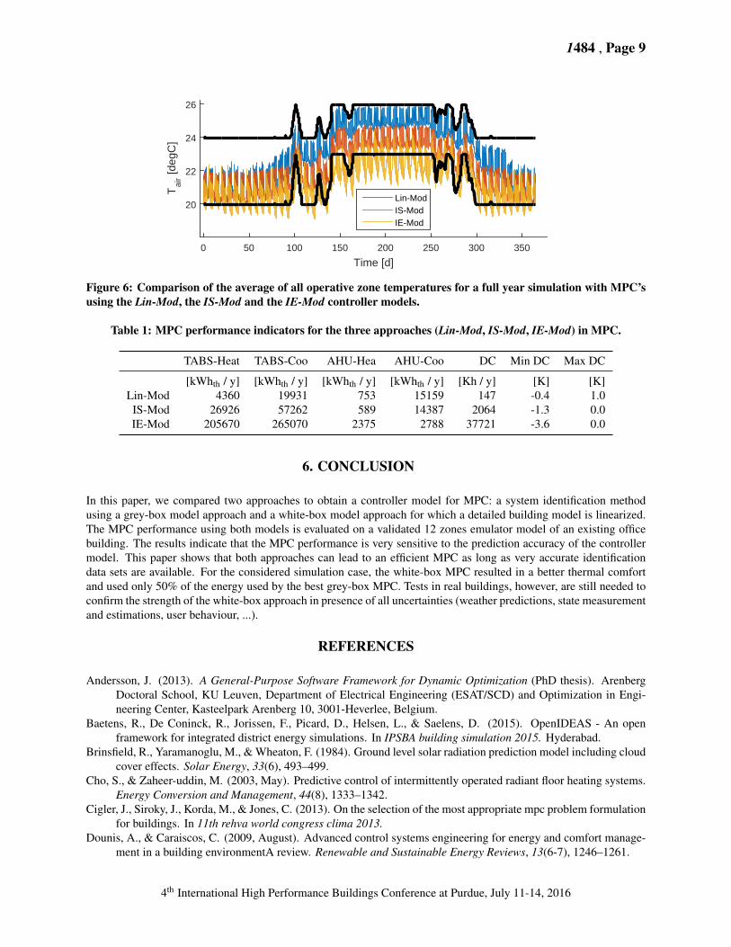
The MPC formulation is used with the different controller models to control the building climate during a full yearsimulation. Fig. 6 shows the average of the 12 operative temperatures as calculated by the emulator for the differentMPCs together with the lower and upper indicators temperature bounds. Table 1 summarizes the MPC performancefactors for the whole building for each MPC, i.e. the heating and cooling energy used by the TABS (TABS-Heat,TABS-Coo) and the ventilation (AHU-Hea, AHU-Coo) and the total discomfort (DC) together with the minimal andmaximal deviation from the comfort range.

Figure 6 and Table 1 show that the Lin-Mod MPC is able to keep the operative temperatures within the comfort boundswith only a negligible discomfort of 147 Kh/year and with a punctual maximal deviation of 1 K. The discomfort ismainly due to the model mismatch introduced by Eq. 1b which culminates when the air temperatures differ the mostbetween the zones. When Tair,i is higher than Tair and the ventilation is turned off (i.e. m1 = 0), the MPC constraints setTsup,ven = Tair. Eq. 1b becomes then negative and the MPC supposes that zone i is cooled by the ventilation while thisis in reality not the case. Nevertheless, the discomfort caused by Lin-Mod MPC is only 7% and 0.4% of the discomfortcaused by IS-Mod MPC and IE-Mod MPC, respectively, while its energy use is 41% and 8% of the energy used in theIS-Mod and ES-Mod approaches, respectively.

While less energy efficient and comfort are guaranteed, IS-Mod MPC still achieves good comfort with only 2064Kh /year of discomfort (172 Kh / zone / year) and its energy use is only 20% of those of IE-Mod. Due to thesystematic overestimation of the temperatures as shown by Figure 5, IS-Mod MPC is not able to work close to the uppertemperature comfort bound and therefore it cools more than necessary. Furthermore, the TABS control signals exhibit(not shown) too fast oscillations between heating and cooling actions which lead to an inefficiency energy supply tothe building. This bang-bang behavior is caused by the model mismatch and the linear formulation of the objectivefunction. Adding a smoothing term on the inputs in the cost function as proposed by (Cigler et al., 2013) wouldprobably significantly improve the MPC robustness against its prediction errors and so improve its global performance.Figure 5 also shows that errors on the 3 hours ahead prediction are non-negligible which causes regular discomfortwhen the MPC operates close to the bounds. The maximum deviation of -1.3 K remains, however, acceptable.

Finally, IE-Mod MPC shows poor comfort and a total energy use of 476 MWh while the energy use when the buildingmodel is controlled by the original rule-based-controller (not explained in the text) stays below 240 MWh. Thisconfirms that due to the lack of ’rich’ measurement data, the identified model IE-Mod is not reliable enough to be usedin an MPC. The collection of ’rich’ data (containing enough information for system identification) in real practice isthus a topic for further research, next to testing these approaches in real buildings.

4th International High Performance Buildings Conference at Purdue, July 11-14, 2016

1484 , Page 9

Time [d]0 50 100 150 200 250 300 350

Tai

r [deg

C]

20

22

24

26

Lin-ModIS-ModIE-Mod

Figure 6: Comparison of the average of all operative zone temperatures for a full year simulation with MPC’susing the Lin-Mod, the IS-Mod and the IE-Mod controller models.

Table 1: MPC performance indicators for the three approaches (Lin-Mod, IS-Mod, IE-Mod) in MPC.

TABS-Heat TABS-Coo AHU-Hea AHU-Coo DC Min DC Max DC

[kWhth / y] [kWhth / y] [kWhth / y] [kWhth / y] [Kh / y] [K] [K]Lin-Mod 4360 19931 753 15159 147 -0.4 1.0

IS-Mod 26926 57262 589 14387 2064 -1.3 0.0IE-Mod 205670 265070 2375 2788 37721 -3.6 0.0

6. CONCLUSION

In this paper, we compared two approaches to obtain a controller model for MPC: a system identification methodusing a grey-box model approach and a white-box model approach for which a detailed building model is linearized.The MPC performance using both models is evaluated on a validated 12 zones emulator model of an existing officebuilding. The results indicate that the MPC performance is very sensitive to the prediction accuracy of the controllermodel. This paper shows that both approaches can lead to an efficient MPC as long as very accurate identificationdata sets are available. For the considered simulation case, the white-box MPC resulted in a better thermal comfortand used only 50% of the energy used by the best grey-box MPC. Tests in real buildings, however, are still needed toconfirm the strength of the white-box approach in presence of all uncertainties (weather predictions, state measurementand estimations, user behaviour, ...).

REFERENCES

Andersson, J. (2013). A General-Purpose Software Framework for Dynamic Optimization (PhD thesis). ArenbergDoctoral School, KU Leuven, Department of Electrical Engineering (ESAT/SCD) and Optimization in Engi-neering Center, Kasteelpark Arenberg 10, 3001-Heverlee, Belgium.

Baetens, R., De Coninck, R., Jorissen, F., Picard, D., Helsen, L., & Saelens, D. (2015). OpenIDEAS - An openframework for integrated district energy simulations. In IPSBA building simulation 2015. Hyderabad.

Brinsfield, R., Yaramanoglu, M., & Wheaton, F. (1984). Ground level solar radiation prediction model including cloudcover effects. Solar Energy, 33(6), 493–499.

Cho, S., & Zaheer-uddin, M. (2003, May). Predictive control of intermittently operated radiant floor heating systems.Energy Conversion and Management, 44(8), 1333–1342.

Cigler, J., Siroky, J., Korda, M., & Jones, C. (2013). On the selection of the most appropriate mpc problem formulationfor buildings. In 11th rehva world congress clima 2013.

Dounis, A., & Caraiscos, C. (2009, August). Advanced control systems engineering for energy and comfort manage-ment in a building environmentA review. Renewable and Sustainable Energy Reviews, 13(6-7), 1246–1261.

4th International High Performance Buildings Conference at Purdue, July 11-14, 2016

1484 , Page 10

Gwerder, M., & Todtli, J. (2005). Predictive Control for Thermal Storage Management in Buildings. In 8th REHVAworld congress for building technologies - CLIMA (pp. 1–6). Lausanne.

Gyalistras, D., & Gwerder, M. (2009). Use of weather and occupancy forecasts for optimal building climate control(opticontrol), two years progress report. (Tech. Rep.). Terrestrial Systems Ecology ETH Zurich.

Hilliard, T., Kavgic, M., & Swan, L. (2015). Model predictive control for commercial buildings: trends and opportu-nities. Advances in Building Energy Research, 1–19.

Ihm, P., & Krarti, M. (2005). Optimal Control Strategies for Heated Radiant Floor Systems. ASHRAE Transactions,535–546.

Jorissen, F., & Helsen, L. (2016). Towards and automated tool chain for MPC in multi-zone buildings, submitted. In2016 intelligent building operations workshop. West Lafayette.

Karlsson, H. (2006). Thermal system analysis of embedded building integrated heating (Unpublished doctoral disser-tation). Chalmers University of Technology.

Ma, Y., Kelman, A., Daly, A., & Borrelli, F. (2012, Feb). Predictive control for energy efficient buildings withthermal storage: Modeling, stimulation, and experiments. IEEE Control Systems, 32(1), 44-64. doi: 10.1109/MCS.2011.2172532

Maciejowski, J. M. (2002). Predictive Control with Constraints. Harlow, Essex: Pearson Education Limitedl.Meteotest. (2009). Meteonorm version 6.1 - edition 2009 [Computer software manual].Morari, M., & Lee, J. H. (1999). Model predictive control : past , present and future. Computers & Chemical

Engineering Engineering, 23, 667–682.Picard, D., Drgona, J., Helsen, L., & Kvasnica, M. (2016). Impact of the plant and controller model complexity on

model predictive control performance evaluation for buildings, submitted. Applied Energy.Picard, D., Jorissen, F., & Helsen, L. (2015). Methodology for obtaining linear state space building energy simulation

models. In 11th international modelica conference (pp. 51–58).Privara, S., Cigler, J., Vana, Z., Oldewurtel, F., Sagerschnig, C., & Zacekova, E. (2013, JAN). Building modeling as

a crucial part for building predictive control. Energy & Buildings, 56, 8-22. doi: {10.1016/j.enbuild.2012.10.024}

Prıvara, S., Siroky, J., Ferkl, L., & Cigler, J. (2011, February). Model predictive control of a building heating system:The first experience. Energy & Buildings, 43(2-3), 564–572.

Pyephem. (2016). https://pypi.python.org/pypi/pyephem/. (Accessed: 2016-04-28)

ACKNOWLEDGEMENT

The Authors gratefully acknowledge the financial support of the of the Scientific Grant Agency of the Slovak Republicunder the grants 1/0403/15. The authors also acknowledge the financial support by the Agency for Innovation byScience and Technology in Flanders (IWT) and WTCB in the frame of the IWT-VIS Traject SMART GEOTHERMfocusing on integration of thermal energy storage and thermal inertia in geothermal concepts for smart heating andcooling of (medium) large buildings, as well as the financial support of the Ph.D. work of Filip Jorissen (IWT 131012Ph.D. Grant), and the EU for funding the research work of Maarten Sourbron.

4th International High Performance Buildings Conference at Purdue, July 11-14, 2016