Comparison of implicit and explicit procedures -...
36
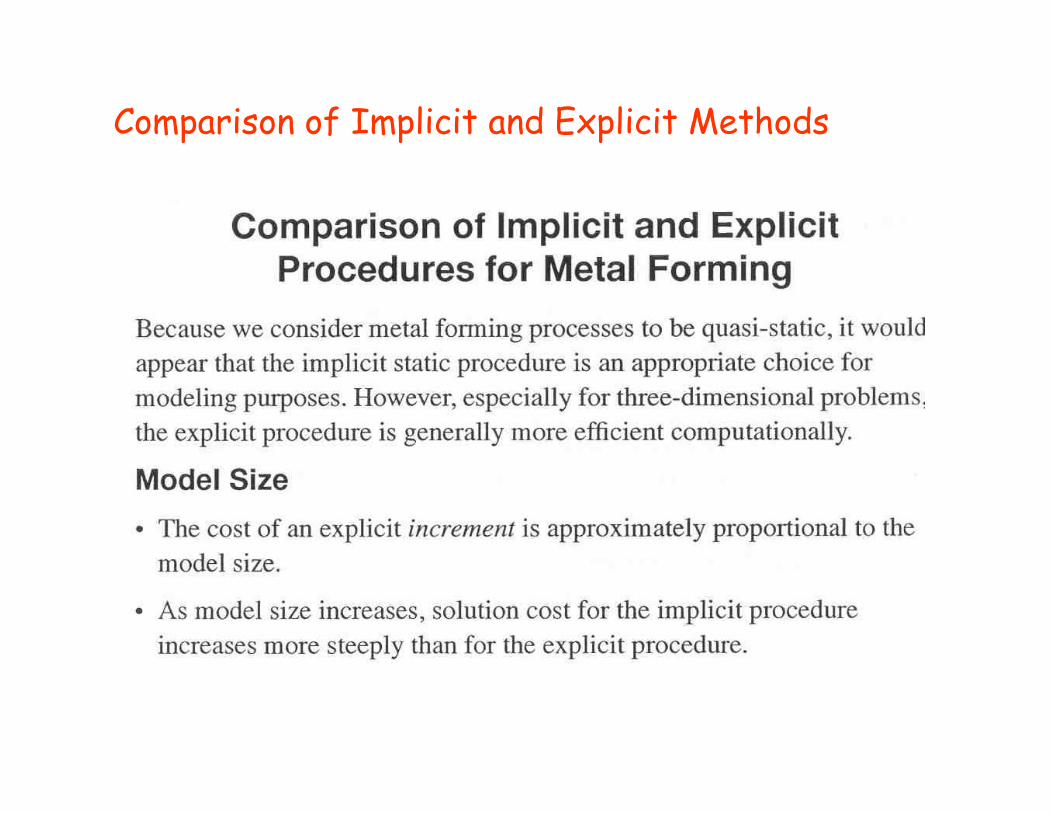
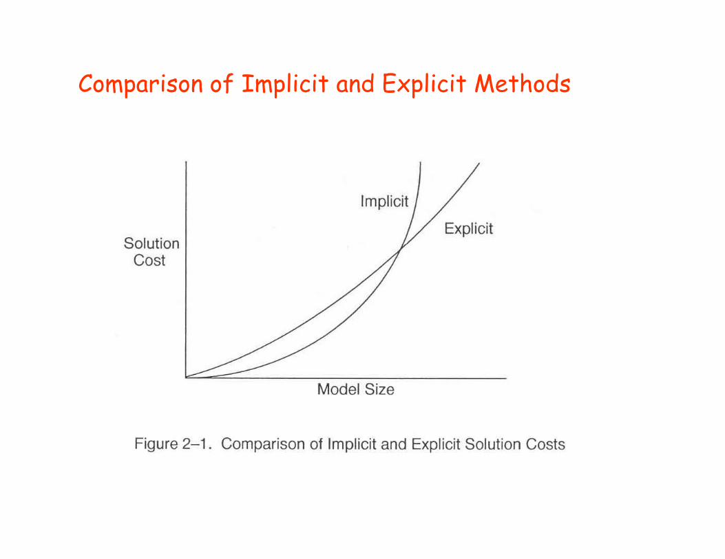
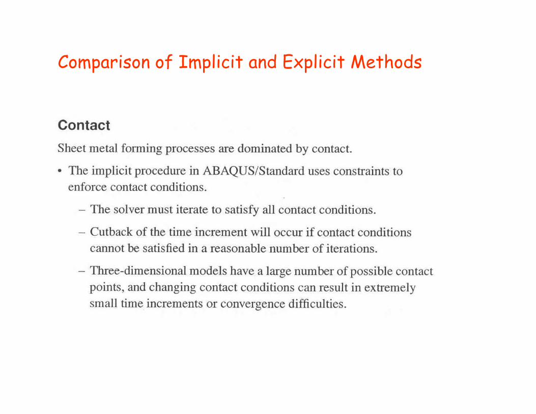
Comparison of implicit and explicit procedures Abaqus/Standard is more efficient for solving smooth nonlinear problems; on the other hand, Abaqus/Explicit is the clear choice for a wave propagation analysis. There are, however, certain static or quasi-static problems that can be simulated well with either program. Typically, these are problems that usually would be solved with Abaqus/Standard but may have difficulty converging because of contact or material complexities, resulting i l b f it ti S h l i i ina large number of iterations. Such analyses are expensive in Abaqus/Standard because each iteration requires a large set of linear equations to be solved.
Transcript of Comparison of implicit and explicit procedures -...
Comparison of implicit and explicit procedures
Abaqus/Standard is more efficient for solving smooth nonlinearproblems; on the other hand, Abaqus/Explicit is the clear choicefor a wave propagation analysis. There are, however, certainstatic or quasi-static problems that can be simulated well witheither program. Typically, these are problems that usually woulde ther program. Typ cally, these are problems that usually wouldbe solved with Abaqus/Standard but may have difficultyconverging because of contact or material complexities, resultingi l b f it ti S h l i iin a large number of iterations. Such analyses are expensive inAbaqus/Standard because each iteration requires a large set oflinear equations to be solved.q
Comparison of implicit and explicit procedures
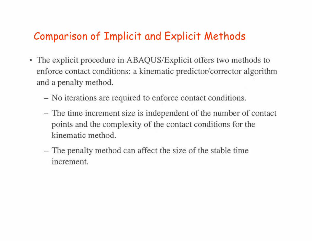
Whereas Abaqus/Standard must iterate to determine thesolution to a nonlinear problem, Abaqus/Explicit determines thesolution without iterating by explicitly advancing the kinematicstate from the previous increment. Even though a given analysismay require a large number of time increments using the explicitmay requ re a large number of t me ncrements us ng the expl c tmethod, the analysis can be more efficient in Abaqus/Explicit ifthe same analysis in Abaqus/Standard requires many iterations.
Another advantage of Abaqus/Explicit is that it requires muchless disk space and memory than Abaqus/Standard for the samep y qsimulation. For problems in which the computational cost of thetwo programs may be comparable, the substantial disk space andmemory savin s of Abaqus/Explicit make it attractivememory savings of Abaqus/Explicit make it attractive.
Comparison of Implicit and Explicit Methods
Comparison of Implicit and Explicit Methods
Comparison of Implicit and Explicit Methods
Comparison of Implicit and Explicit Methods
Comparison of Implicit and Explicit Methods
Comparison of Implicit and Explicit Methods
Comparison of Implicit and Explicit Methods
Comparison of Implicit and Explicit Methods

Comparison of Implicit and Explicit Methods
Comparison of Implicit and Explicit Methods
Comparison of Implicit and Explicit Methods
Comparison of Implicit and Explicit Methods
Comparison of Implicit and Explicit Methods
Comparison of Implicit and Explicit Methods
Comparison of Implicit and Explicit Methods
Comparison of Implicit and Explicit Methods
Comparison of Implicit and Explicit Methods
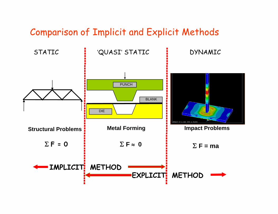
STATIC ‘QUASI’ STATIC DYNAMIC
PUNCH
DIE
BLANK
Structural Problems Metal Forming Impact Problems
Σ F = 0 Σ F ≈ 0 Σ F = maΣ F ma
IMPLICIT METHODEXPLICIT METHODEXPLICIT METHOD
Comparison of Implicit and Explicit Methods
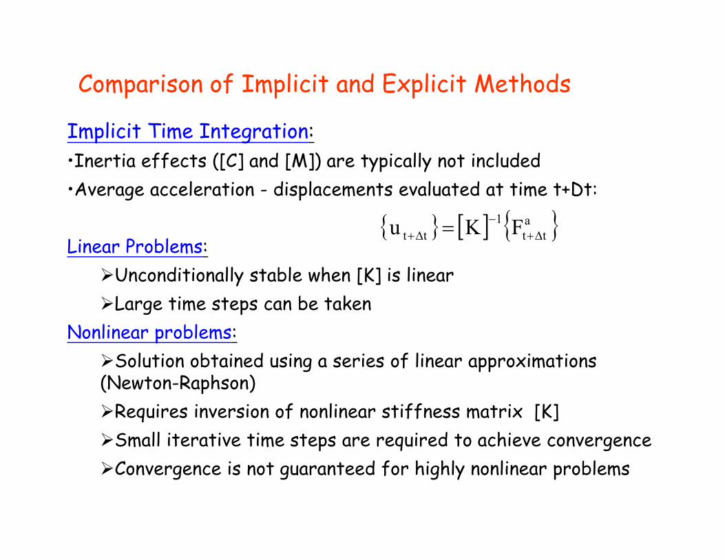
Implicit Time Integration:•Inertia effects ([C] and [M]) are typically not included •Average acceleration - displacements evaluated at time t+Dt:
Linear Problems:{ } [ ] { }a
tt1
tt FKu Δ+−
Δ+ =Linear Problems:
Unconditionally stable when [K] is linearLarge time steps can be taken
Nonlinear problems:Solution obtained using a series of linear approximations
(Newton-Raphson)(Newton Raphson)Requires inversion of nonlinear stiffness matrix [K]Small iterative time steps are required to achieve convergenceConvergence is not guaranteed for highly nonlinear problems
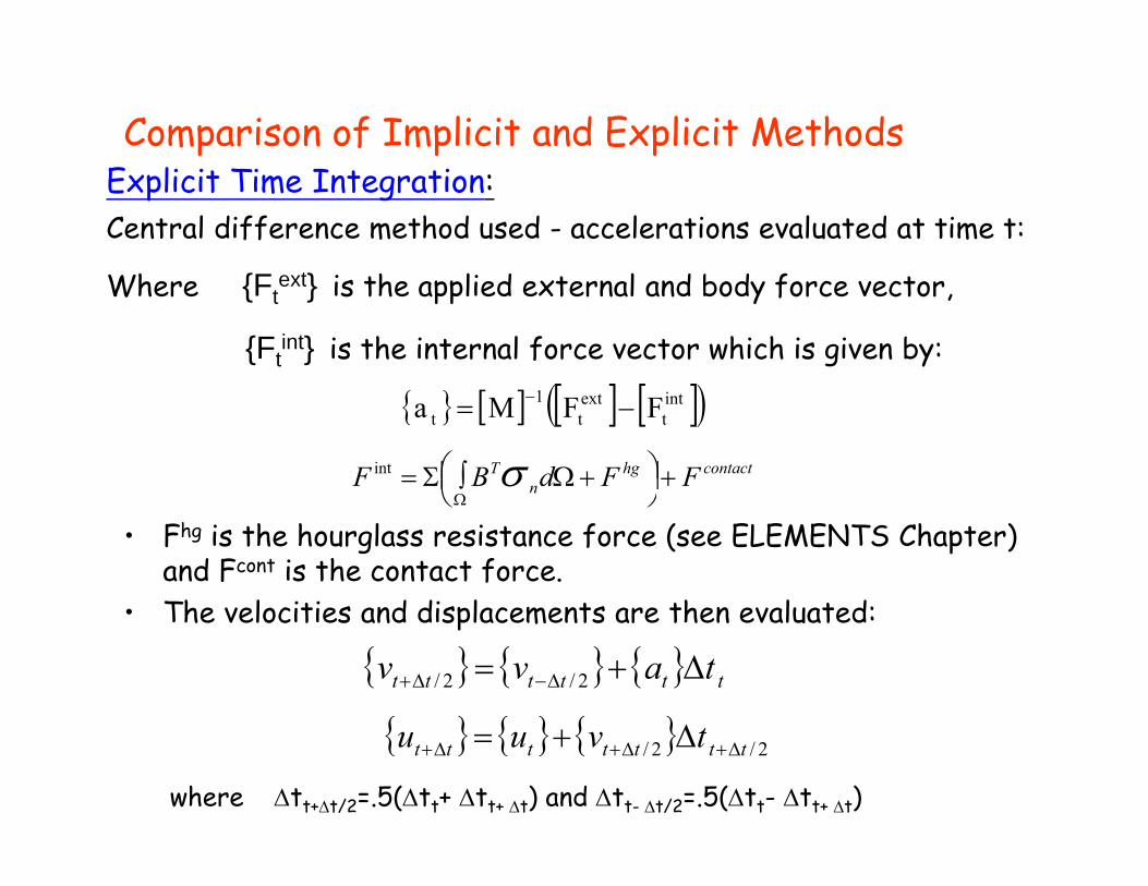
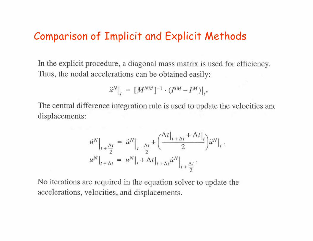
Comparison of Implicit and Explicit MethodsExplicit Time Integration:Central difference method used - accelerations evaluated at time t:
Wh {F ext} i h li d l d b d f Where {Ftext} is the applied external and body force vector,
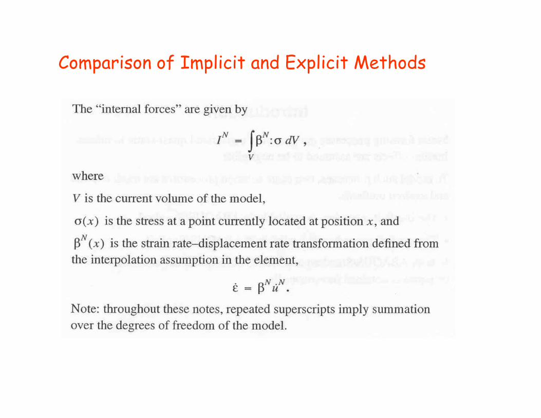
{Ftint} is the internal force vector which is given by:
[ ] [ ]( ){ } [ ] [ ] [ ]( )intt
extt
1t FFMa −= −
contacthgn
T FFdBF +⎟⎠⎞⎜
⎝⎛ +Ω∫Σ=
Ωσint
⎠⎝ Ω
• Fhg is the hourglass resistance force (see ELEMENTS Chapter) and Fcont is the contact force.
• The velocities and displacements are then evaluated:• The velocities and displacements are then evaluated:
{ } { } { } tttttt tavv Δ+= Δ−Δ+ 2/2/
{ } { } { }{ } { } { } 2/2/ ttttttt tvuu Δ+Δ+Δ+ Δ+=
where Δtt+Δt/2=.5(Δtt+ Δtt+ Δt) and Δtt- Δt/2=.5(Δtt- Δtt+ Δt)
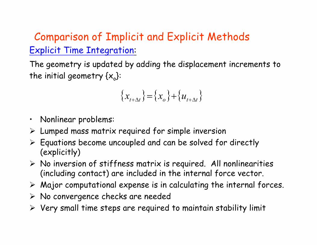
Comparison of Implicit and Explicit MethodsExplicit Time Integration:The geometry is updated by adding the displacement increments to the initial geometry {x }:the initial geometry {xo}:
{ } { } { }ttott uxx Δ+Δ+ +=
• Nonlinear problems:Lumped mass matrix required for simple inversionEquations become uncoupled and can be solved for directly (explicitly)No inversion of stiffness matrix is required. All nonlinearities (including contact) are included in the internal force vector.Major computational expense is in calculating the internal forces.No convergence checks are neededgVery small time steps are required to maintain stability limit

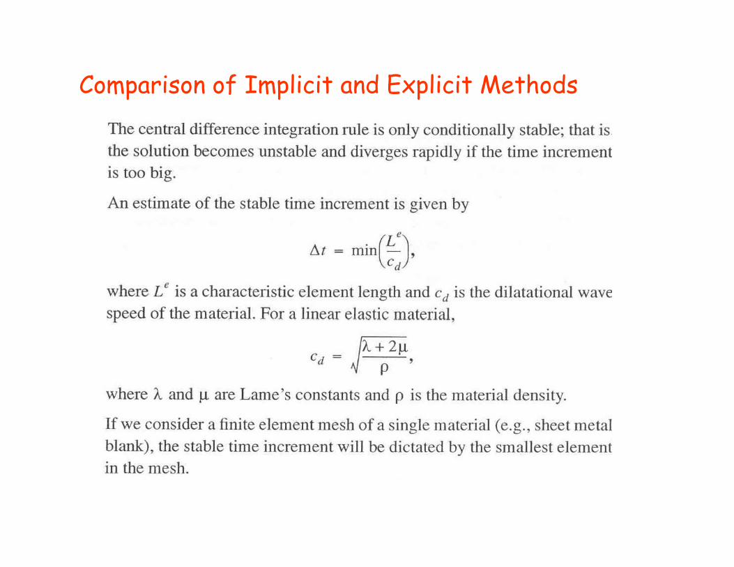
Stability LimitExplicit Time Integration:
Only stable if time step size i ll th iti l ti
Implicit Time Integration:
For linear problems, the time t b bit il l is smaller than critical time
step size
Δ Δ crit 2
step can be arbitrarily large (always stable)
For nonlinear problems time Δ Δt t crit≤ =ωmax
For nonlinear problems, time step size may become small due to convergence difficulties
Where wmax = largest natural circular frequency
Due to this very small time step size, explicit is useful only for very short transientsonly for very short transients
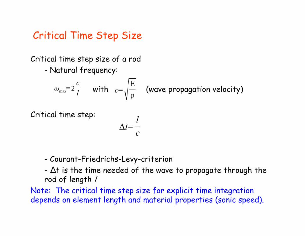
Critical Time Step Size
Critical time step size of a rod - Natural frequency:q y
lc
=ω 2max withρE
c= (wave propagation velocity)
Critical time step:
cl
t=Δ
- Courant-Friedrichs-Levy-criterion
c
y- ∆t is the time needed of the wave to propagate through the rod of length l
Note: The critical time step size for explicit time integration Note: The critical time step size for explicit time integration depends on element length and material properties (sonic speed).
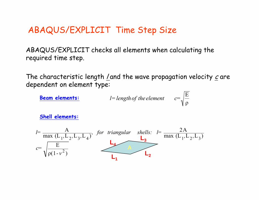
ABAQUS/EXPLICIT Time Step Size
ABAQUS/EXPLICIT checks all elements when calculating the required time step.
The characteristic length l and the wave propagation velocity c are dependent on element type:p yp
ρEc=elementtheoflength=lBeam elements:
)LL(LmaxA2
)LLL(LmaxA
3214321 ,,l=shells: triangular for ,,,,l=L
Shell elements:
)-1ρ(E
)()(
2
3214321
νc=
,,,,,
L1
L4L3
L2
A
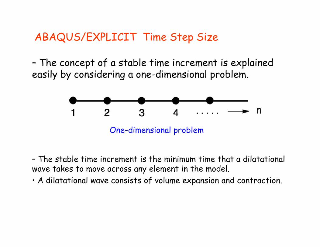
ABAQUS/EXPLICIT Time Step Size
– The concept of a stable time increment is explained easily by considering a one-dimensional problem.easily by considering a one dimensional problem.
One-dimensional problem
– The stable time increment is the minimum time that a dilatational wave takes to move across any element in the modelwave takes to move across any element in the model.• A dilatational wave consists of volume expansion and contraction.
ABAQUS/EXPLICIT Time Step Size
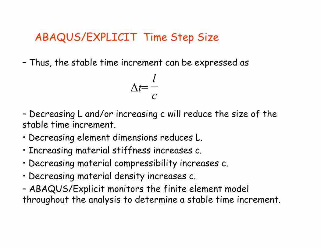
– Thus, the stable time increment can be expressed as
lcl
t=Δ
– Decreasing L and/or increasing c will reduce the size of the stable time increment.• Decreasing element dimensions reduces L Decreasing element dimensions reduces L.• Increasing material stiffness increases c.• Decreasing material compressibility increases c.• Decreasing material density increases c.– ABAQUS/Explicit monitors the finite element model throughout the analysis to determine a stable time increment.throughout the analysis to determine a stable time increment.
Summary

Summary
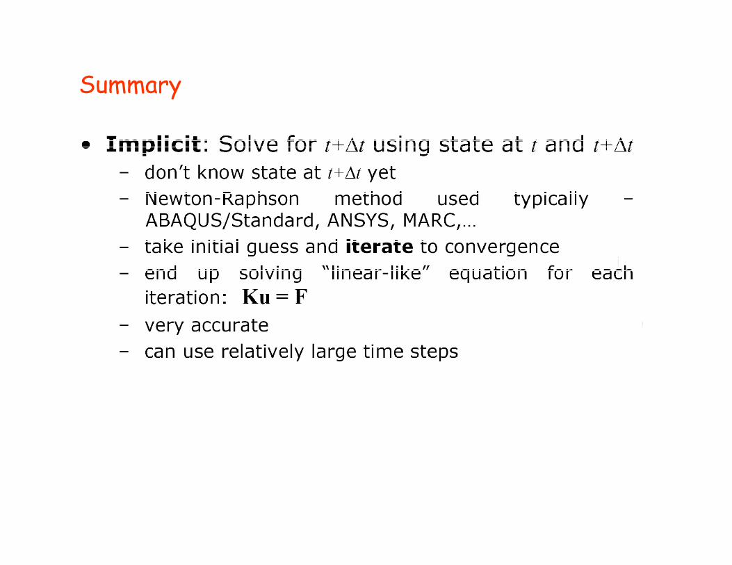
Implicit Time Integration (used by ANSYS) -
El •Finite Element method used
•Average acceleration calculated
•Displacements evaluated•Displacements evaluated
•Always stable – but small time steps needed to capture transient response
•Non-linear materials can be used to solve static problems
•Can solve non-linear (transient) problems…
•…but only for linear material properties
•Best for static or ‘quasi’ static problems
Summary
Summary
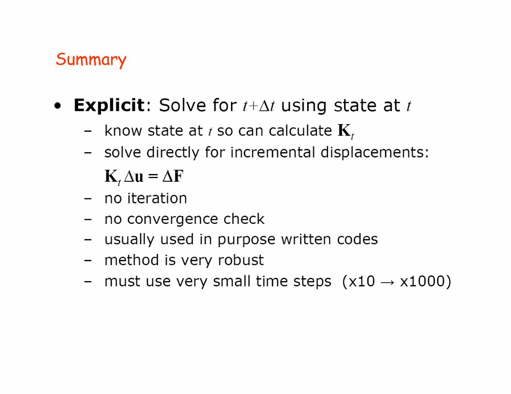
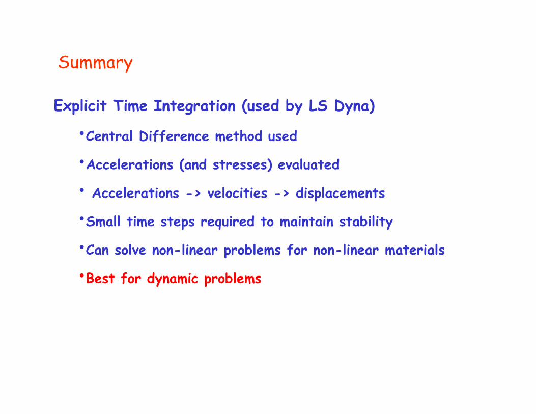
Explicit Time Integration (used by LS Dyna)
•Central Difference method used
•Accelerations (and stresses) evaluated
• Accelerations -> velocities -> displacements
•Small time steps required to maintain stability
•Can solve non-linear problems for non-linear materials
•Best for dynamic problemsy p
Overview of the Explicit Dynamics Procedurep y
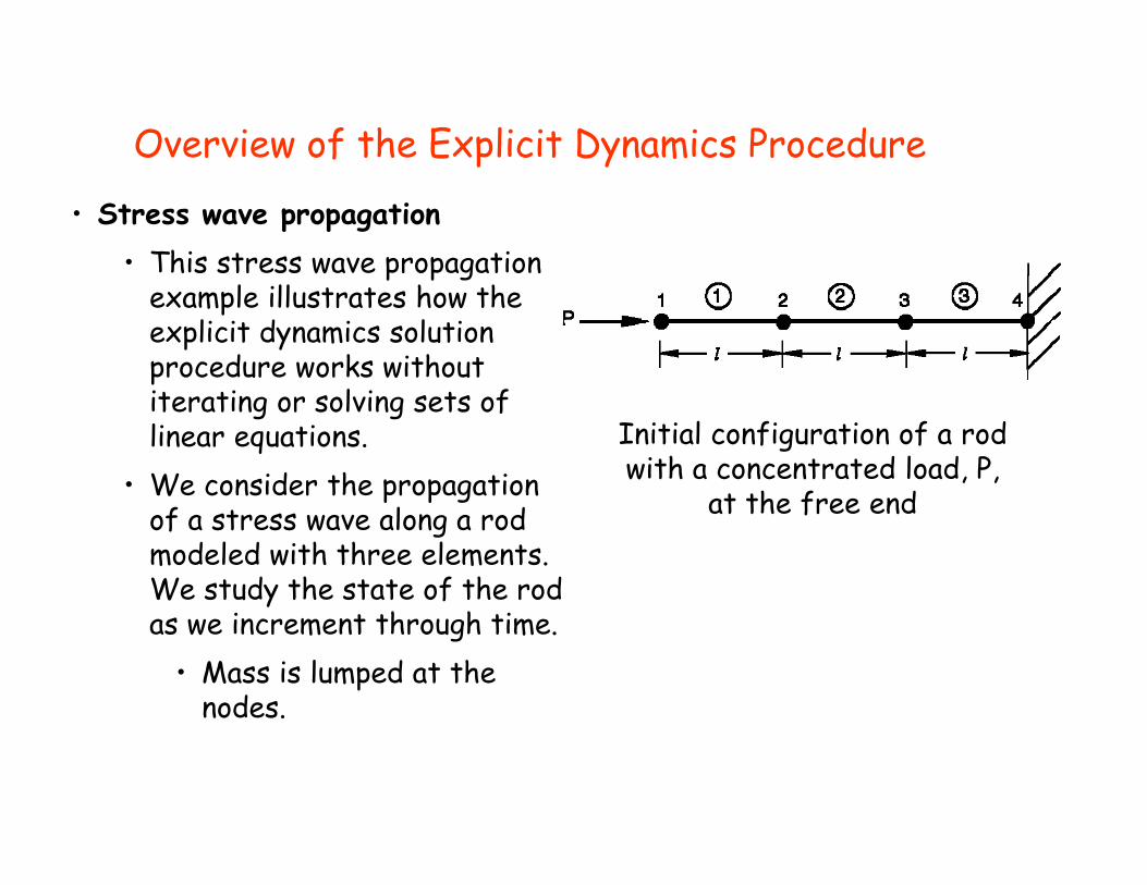
• Stress wave propagation• This stress wave propagation p p g
example illustrates how the explicit dynamics solution procedure works without iterating or solving sets of linear equations.
• We consider the propagation
Initial configuration of a rod with a concentrated load, P,
at the free endp p gof a stress wave along a rod modeled with three elements. We study the state of the rod
at the free end
as we increment through time. • Mass is lumped at the
nodes.
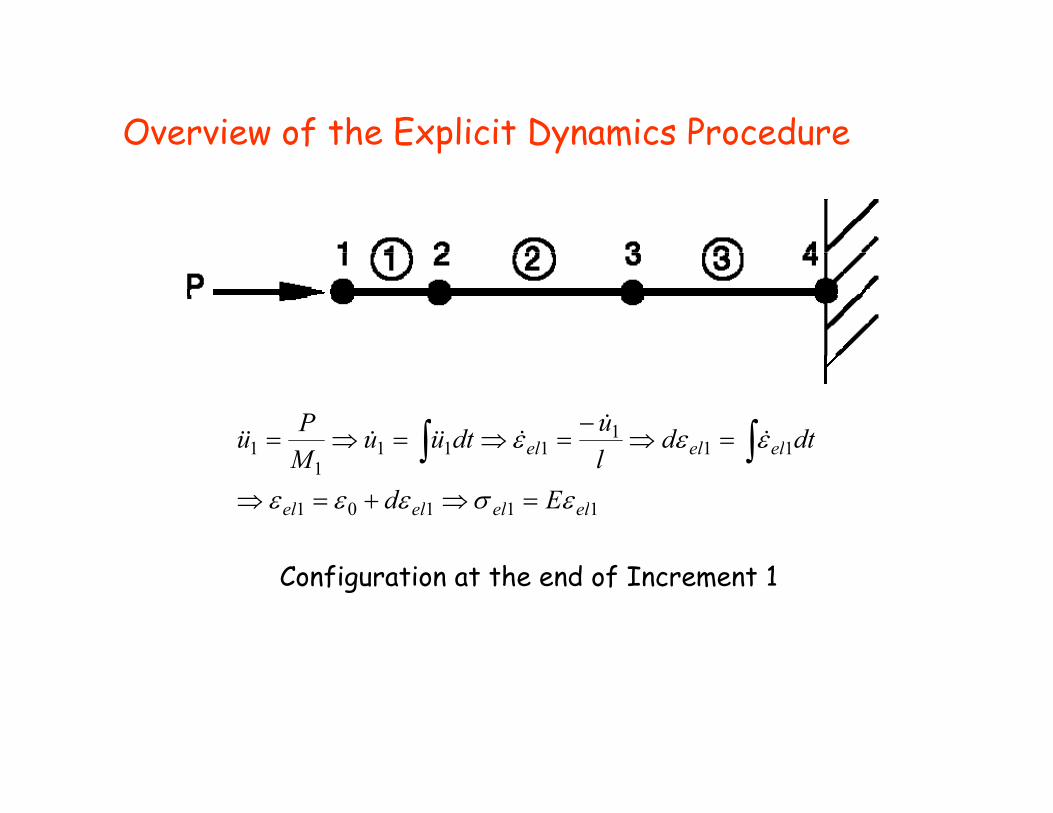
Overview of the Explicit Dynamics Procedurep y
111
1111 elelel dtdludtuu
MPu εεε =⇒
−=⇒=⇒= ∫ ∫ &
&&&&&&&
11101
1
elelelel EdlM
εσεεε =⇒+=⇒
∫ ∫
Configuration at the end of Increment 1
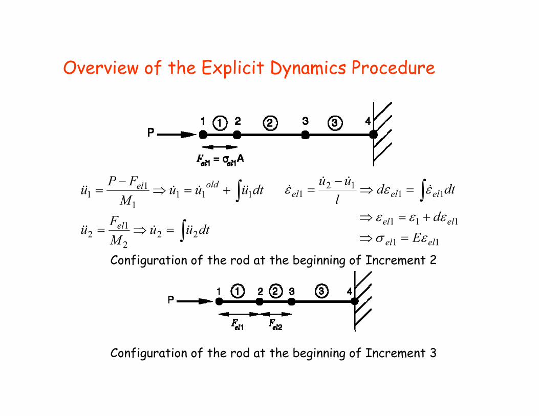
Overview of the Explicit Dynamics Procedurep y
∫− FP ld ∫
− uu &&
∫
∫=⇒=
+=⇒−
=
dtuuFu
dtuuuM
FPu
el
oldel
221
2
1111
11
&&&&&
&&&&&&
111 elel
Edεεε +=⇒
∫=⇒= dtdl
uuelelel 11
121 εεε &&
Configuration of the rod at the beginning of Increment 2
∫M 222
211 elel Eεσ =⇒
Configuration of the rod at the beginning of Increment 3
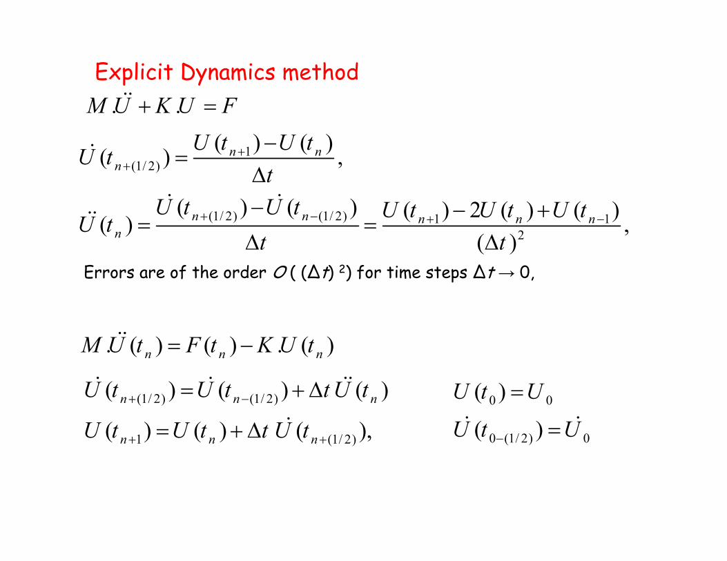
M U K U F+&&Explicit Dynamics method
1(1/ 2)
( ) ( )( ) ,n nn
U t U tU tt
++
−=
Δ&
. .M U K U F+ =
(1/ 2) (1/ 2) 1 12
( ) ( ) ( ) 2 ( ) ( )( ) ,( )
n n n n nn
tU t U t U t U t U tU t
t t+ − + −
Δ− − +
= =Δ Δ
& &&&
( )t tΔ ΔErrors are of the order O ( (∆t) 2) for time steps ∆t → 0,
( ) ( ) ( )U t U t t U t+ Δ& & &&
. ( ) ( ) . ( )n n nM U t F t K U t= −&&
( )U t U(1/ 2) (1/ 2)
1 (1/ 2)
( ) ( ) ( )
( ) ( ) ( ),n n n
n n n
U t U t t U t
U t U t t U t+ −
+ +
= + Δ
= + Δ &0 0
0 (1/ 2) 0
( )
( )
U t U
U t U−
=
=& &
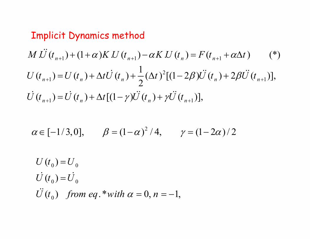
Implicit Dynamics method
1 1 1
2
. ( ) (1 ) . ( ) . ( ) ( ) (*)1( ) ( ) ( ) ( ) [(1 2 ) ( ) 2 ( )]
n n n nM U t K U t K U t F t t
U t U t tU t t U t U t
α α α
β β
+ + ++ + − = + Δ
+ Δ + Δ +
&&
& && &&1 1
1 1
( ) ( ) ( ) ( ) [(1 2 ) ( ) 2 ( )],2
( ) ( ) [(1 ) ( ) ( )],
n n n n n
n n n n
U t U t tU t t U t U t
U t U t t U t U t
β β
γ γ
+ +
+ +
= + Δ + Δ − +
= + Δ − +& & && &&
2[ 1/ 3,0], (1 ) / 4, (1 2 ) / 2α β α γ α∈ − = − = −
0 0( )U t U=
[ 1/ 3,0], (1 ) / 4, (1 2 ) / 2α β α γ α∈
0 0
0 0
( )
( )
( ) * 0 1
U U
U t U
U t from eq with nα
=
= = −
& &
&&0( ) . 0, 1,U t from eq with nα = =